Topology of the mesoscale connectome of the mouse brain
Pascal Grange
Xi’an Jiaotong-Liverpool University, Department of Mathematical Sciences, Suzhou, China
Pascal.Grange@xjtlu.edu.cn
Abstract
The wiring diagram of the mouse brain has recently been mapped at a mesoscopic scale in the Allen Mouse Brain Connectivity Atlas. Axonal projections from brain regions were traced using green fluoresent proteins. The resulting data were registered to a common three-dimensional reference space. They yielded a matrix of connection strengths between 213 brain regions. Global features such as closed loops formed by connections of similar intensity can be inferred using tools from persistent homology. In this paper the wiring diagram of the mouse brain is mapped to a simplicial complex (filtered by connection strength), and generators of the first homology group are computed. Some regions, including nucleus accumbens, are connected to the entire brain by loops. Thousands of loops go through the isocortex, the striatum and the thalamus. On the other hand, medulla is the only major brain compartment that contains more than 100 loops.
1 Introduction
The Allen Mouse Brain Connectivity Atlas [1] has filled a major
gap in the knowledge of neuroanatomy by providing a brain-wide
map of the connectome of the mouse brain. Adeno-associated
viral vectors expressing enhanced green fluorescent protein were injected into the mouse brain, allowing to trace axonal projections.
The scale of these experiments is mesoscopic [2], in the sense that injections target groups of neurons
belonging to brain regions assumed to be homogeneous. The microscopic
scale would correspond to mapping individual synapses where neurons make contact.
The resulting three-dimensional fluorescent traces were registered to brain regions
defined in the hierarchical Allen Reference Atlas [3].
These results allowed the construction of the first inter-region connectivity model of the mouse brain.
It takes the form of a connectivity matrix,
whose rows and columns correspond to a brain region, and whose entries model the connection strengths
between pairs of regions defined by classical neuroanatomy. The derivation
of the entries of of the connectivity matrix assumed homogeneity of brain regions and additivity of connection strengths.
Projection densities correspond to axons
highlighted by tracers, hence the projection densities
from several different sources sum to produce projection density in a given region. This additivity assumption was used to address experimental data
in which an injection of viral tracer infected several neighbouring brain regions.
The construction
of the model from injection data (possibly infecting several regions for each injection) assumes that projections
are homogeneous in each region, and that projections from different sources add to produce projection density
to a given region. The entries of the connectivity matrix were observed to span a -fold range, and are approximately
fit by a log-normal distribution.
The connectivity matrix is naturally mapped to a graph that models the wiring diagram of the mouse brain.
Some features of the wiring diagram
such as node degree and clustering coefficient have been observed to be reproduced by scale-free networks [4] and
small-world networks [5], but none of these models was found to fit all observed features of the wiring diagram.
This begs for further modelling taking into account the global properties of the
connectivity map, together with the large range of intensities mapped by connection strengths.
On the other hand, the recent computational developments of algebraic topology [6, 7, 8, 9] have given rise to spectacular applications to data analysis in biological sciences, including obstructions to phylogeny in viral evolution [10], and brain networks and neural correlations [11, 12, 13, 14, 15]. In this paper we will apply techniques from algebraic topology, a branch of mathematics characterizing properties of spaces that are invariant by continuous deformation, to work out global properties of the wiring diagram of the mouse brain.
We will first review the presentation of the Allen Mouse Brain Connectivity Atlas in the form of a matrix modelling connection strengths between brain regions. We will define a mapping from these data to a filtered simplicial complex and explain why the generators of the first homology group are in one-to-one correspondence with closed loops in the mesoscale connectome. The anatomy of these loops will then be analysed by grouping loops according to the major brain compartments they intersect. Moreover, we will compare the fraction of the brain reached from each region by loops, to the fraction reached by direct connections encoded in the connectivity matrix.
2 Materials and methods
2.1 Connectivity strengths in the mouse brain, local and global properties
Each image series in the Allen Mouse Connectivity Atlas corresponds to an injection of tracer, followed by sectioning and and imaging of the brain11 1 © 2014 Allen Institute for Brain Science. Allen Connectivity Atlas. Available from: http://connectivity.brain-map.org/.org. In [1], registered data from 469 image series were combined in order to estimate an inter-region connectivity matrix, presented in matrix form22 2 The entries of the matrix correspond to the left-hand side of Fig. 3 in [1].:
| (1) |
The size of this connectivity matrix is , and each of the indices in corresponds to a brain region,
defined in the
Allen Reference Atlas (ARA, [3, 16]).
The connectivity matrix captures the local structure of the connectome at mesocopic scale,
as it estimates the strength of direct connections from a region to other regions. To capture global
features of the connectome, we would like to identify closed circuits constructed from these connections.
Algebraic topology formalises this notion: an irreducible closed loop in a topological space (a loop that cannot be shrunk to a point
by continuous deformations) is a loop that is not the boundary of a disc in the topological space. It
is therefore a one-dimensional cycle that is not the boundary of a two-dimensional object. The family
of such objects in a topological space is invariant by continuous deformation, and has a group structure. It is called the
first homology group of the topological space, and denoted by .
If we repeat this reasoning in dimension zero, we obtain the more familiar notion of connected component: elements of
are zero-dimensional objects that cannot
be joined by a path drawn on the topological space. They correspond to distinct connected components.
More generally, the elements of the homology group are objects of dimension that are not boundaries of -dimensional
objects in a topological space, and therefore formalise the notion of hole.
Moreover, the algebraic structure of homology groups allows us to count independent objects in each of them: the number of generators of the homology group
is called the -th Betti number and denoted by . The Betti numbers and are the
number of connected components and the number of independent loops respectively.
2.2 Mapping the matrix of connection strengths to a filtered simplicial complex
The connectivity matrix is not symmetric, because projections from a given brain region to other brain regions are oriented (just as axons are). Let us map the connectivity matrix to a weighted graph with vertices corresponding to brain regions, and weighted edges corresponding to the entries of the connectivity matrix. Edges with two different orientations and different weights can exist between pairs of vertices. Let us apply a decreasing function to the entries of the connectivity matrix and define for instance:
| (2) |
where is a positive regulator chosen to be smaller than the minimum connection strength, so that
entries of are bounded. The families of loops worked out in this paper do not depend on the choice of
(in practice we took , resulting in a maximum entry of for ).
This operation results in an approximately normal distribution of entries in the matrix .
The quantity has been observed in [1] to be positively correlated
to the spatial distance between region labelled and region labelled .
However, the entries of are not quite distances because is not symmetric.
We propose to map brain regions to a graph with vertices as follows.
Each brain region, labelled , is mapped to a
pair of vertices , where represents the sources of action potentials (the axons of the cell bodies in the region, that conduct axon potentials), and
the targets of action potentials (the dendrites in the region, that receive action potentials).
An edge is drawn between vertices and for each in . With this doubling prescription we declare edges between targets and sources to be present in each region. We are going to look for closed paths in the wiring diagram of the brain,
constructed from the non-zero entries of the connection matrix.
Direct approaches to persistent
homology for asymmetric networks have been proposed, based on the Dowker complex, see [17], but the present doubling prescription takes
advantage of the mesoscopic scale of the connectome data.

Given the family of labelled vertices we have just described,
we can construct a family of graphs and work out the families of independent loops for each of them
by executing the following pseudo-code:
1. Consider a fixed (referred to as a filtration value).
2. Draw an edge between any source labelled and any target labelled such that .
3. Work out generators of the homology groups (connected components) and (independent loops) in the resulting graph.
The family of graphs (depending on the parameter ) is called a simplicial complex.
The third step of the procedure uses techniques of simplicial homology, implemented
in JavaPlex [18, 19]. Simplices in our case consist of vertices (zero-simplices, corresponding to brain regions),
and edges (one-simplices, corresponding to axons connecting two brain regions).
The result of the above procedure depends on the value of the filtration value .
At we have as many connected components as points, and no loop. The number of connected components
decreases when increases. It reaches for some value of the filtration value. When is increased beyond this value,
edges may still be drawn, possibly changing the number of loops.
When reaches the maximum entry of the matrix , the simplicial complex cannot be changed anymore by increasing the filtration value.
If we repeat the above procedure for all values of the entries of the matrix , arranged
in increasing order, we can work out for each feature (which can be a connected component or a loop) an interval of
filtration values for which the
feature is present. These intervals can be drawn for all existing features of a fixed dimension, yielding
graphs of barcode form, one per dimension of feature (see Fig. 1B).
Features persistent over a longer interval are thought less likely to be due to noise [20]. In particular, we will restrict ourselves to
cycles that persist from their first appearance (at a given filtration value) to the maximum entry of
the matrix . The results of the above procedure are sketched of Fig. 1 for a toy model
consisting of three regions (and connection strengths assumed to be mapped to ). The pseudo-code
is executed for each unique value of the entries of , in ascending order.
2.3 Neuroanatomy of cycles
2.3.1 Three-dimensional presentation of brain regions
To analyse the anatomy of persistent cycles,
we used the voxelised version of the Allen Reference Atlas at a spatial
resolution of 25 microns 33
3
See download instructions and code snippets in MATLAB and Python on the Allen Brain Atlas data portal:
http://help.brain-map.org/display/mouseconnectivity/API#API-DownloadAtlas3-DReferenceModels .
This three-dimensional grid contains numerical labels encoding neuroanatomy at the
finest level compatible with the resolution (the voxelised atlas consists of cubic voxels,
with 677 distinct regions). These numerical labels are associated to the names of brain regions accroding to the hierarchical annotation
of the ARA 44
4
The hierarchical system of annotation containing names of brain regions and numerical ids is available online
at http://api.brain-map.org/api/v2/structure_graph_download/1.json.
For each of the regions in the mesoscale model
of the connectome (Eq. 1), we resolved the numerical label
and the corresponding voxels.
If the region has descendants in the hierarchical annotation,
we lump together the voxels corresponding to these descendants, by annotating them with the
numerical label of the region. After this step, the voxelised atlas contains distinct regions.
The regions included in the mesoscale model of the connectome therefore do not quite span the entire
brain. Let us denote by the number of voxels in region labelled :
| (3) |
The brain regions corresponding to the rows of the connectivity matrix contain
| (4) |
about 79 percent of the total volume of the brain. In the rest of this paper we will disregard the brain
regions that are not included in the matrix of connectivity strengths, and the volume will be referred to as the volume of the
brain.
Grouping
brain regions at a coarse hierarchical level (according to the ARA [3, 16]) yields the following major brain
compartments which will sometimes be designated by acronyms for presentation purposes:
Isocortex, olfactory areas (OLF), cortical subplate (CTXsp), striatum (STR), pallidum (PAL), thalamus (TH),
hypothalamus (HY), midbrain (MB), medulla (MY), cerebellar cortex (CBX). These major brain compartments will be referred to as big regions.
2.3.2 Fraction of the brain connected by loops to a given region
Given a brain region labelled and a filtration value , let us denote by the family of generators of the first homology group at filtration value that go through the region :
| (5) |
and by the set of vertices through which the elements of go:
| (6) |
In the toy model of Fig. 1 with three brain regions, the sets and
are empty. The set consists of one loop, corresponding to .
We can calculate the volume of the regions connected to the region by loops, as a fraction of the total number of voxels in the brain:
| (7) |
where is the total number of voxels defined in Eq. 4, and is the number of voxels in region labelled . As the volumes of brain regions are not all equal, we can define an alternative measure by the fraction of the total number of regions connected to region labelled by loops:
| (8) |
For a region labelled that is connected by loops to all
brain regions, for some value of the filtration , we will have .
It is natural to compare these ratios to the analogous ratios obtained by taking into account only direct connections between pairs of brain regions, as encoded by the connectivity matrix . Let us denote these quantities by for the fraction of volume and by for the fraction of the number of regions:
| (9) |
| (10) |
where denotes the indicator function. By construction the four fractions defined in Eqs 7,8,9,10 are growing functions of the filtration value . There can be regions in the family that are not directly connected to region based on the inter-region connectivity matrix. There can also be regions with projections to or from region that are not involved in any closed cycle going through region at the given filtration value . There is therefore no a priori solidarity between the quantities and , based on loops, and their analogues and , based on direct connections.
2.4 Brain-wide maps of loops going through a given brain region
To sum up the connections by loops between two given brain regions, we can calculate the sum of connection strengths at which cycles connecting these two regions appear, weighted by the numbers of such cycles. As the generators of the first homology groups are independent, this is consistent with the additivity assumption of connection strengths between brain regions. For two regions labelled and we introduce
| (11) |
where the sum is over the distinct filtration values (the distinct entries of the
matrix defined in Eq. 2), and the exponential function comes
from Eq. 2 relating connection strengths to the distance used to
defined filtration values.
Fixing the region label and allowing the region label to take all the possible values in , we can define a brain-wide map of connection strengths to region labelled , by defining for voxel labelled :
| (12) |
where is the index (in ) of the brain region to which voxel labelled belongs.
The quantity maps a voxel to a real number, and can be visualised
as a heat map for instance.
To estimate how localised a brain-wide map of connection strengths is, we can compute the Kullback–Leibler divergence from the above-defined profile and the uniform brain-wide density. If we denote by the label of the region to which voxel labelled belongs, this divergence is expressed as
| (13) |
where is the total number of voxels defined in Eq. 4, and we used the fact that is a normalised density function. This divergence induces a ranking of brain regions.
3 Results
3.1 Persistent cycles
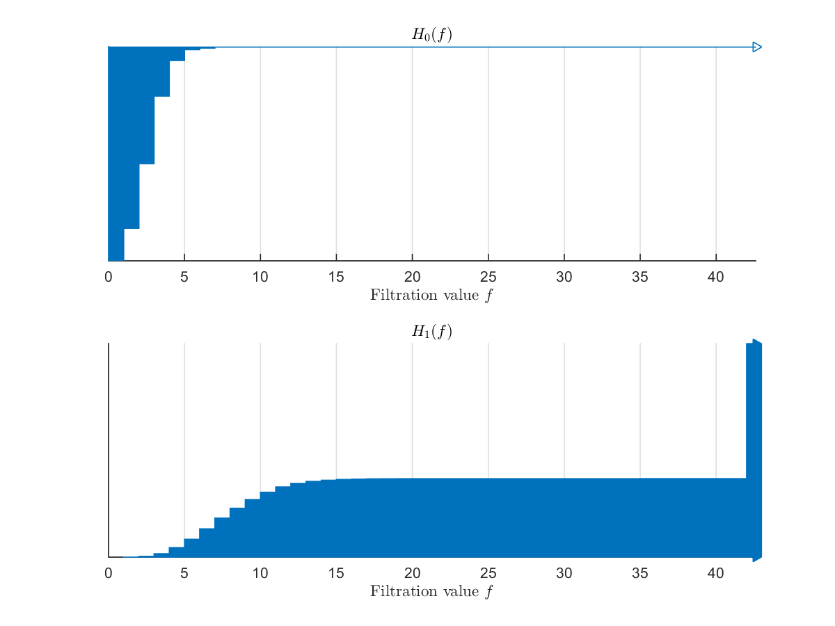
The bar code corresponding to the persistent generators of the first two homology groups is shown in Fig. 2. The maximum Betti numbers are too large for the individual bars to be visible, as they are on Fig. 1B. By construction the Betti number starts at . The Betti number starts at and the plateau at filtration value in the bar code of the first homology group corresponds to . At filtration values larger than , all brain regions are in the same connected component. Moreover, from the growth profile of the bar code of the first homology group, we can see that thousands of persistent cycles appear at filtration values lower than ( at ).
3.2 Loops highlight the cortico-striato-thalamic network
To obtain a coarse picture of the anatomy of cycles,
let us work out which family of big regions (as defined in Section 2.3.1) is intersected by
each loop. We can rank the resulting families of big
regions by decreasing value of prevalence. For an example of the brain regions in a loop appearing at filtration value ,
together with the names of the corresponding big regions, see Table 1. This loop appears at a low filtration
value and we will see that the family of big regions it intersects (isocortex, striatum, thalamus and midbrain) is frequent among loops in the wiring diagram
of the mouse brain.
| Brain region | Big region |
|---|---|
| Anterior cingulate area, dorsal part | Isocortex |
| Primary auditory area | Isocortex |
| Caudoputamen | Striatum |
| Medial geniculate complex, dorsal part | Thalamus |
| Medial geniculate complex, ventral part | Thalamus |
| Superior colliculus, motor related | Midbrain |
Six regions appear, belonging to four distinct big brain regions.
For definiteness we did this calculation at two special filtration values:
- the filtration value at which the Betti number falls to 1.
- the maximum filtration value , above which no extra loops appear (before the value introduced in Eq. 2 to
provide a cut-off to the plots).
We found that distinct families of big regions occur, but the most frequent 27 families account for
50% of the loops.
The most prevalent families of big regions are presented in Table 2 (where they are ordered by decreasing
prevalence at filtration value ). We notice that midbrain is represented in most of the rows of this table55
5
Midbrain is also represented in most of the
loops that appear at low filtration values ., and that the three most frequent combinations (accounting for more than of all the loops)
go through six or more big regions.
The family of four big regions corresponding to the regions in the loop presented in Table 1
is the fourth most prevalent family of big regions in loops appearing at filtration values lower than , with 249 distinct loops (resp. fifth, and 328 loops).
If we focus on small
families of big regions (with three regions or fewer), we observe that the most prevalent is the cortico-striato-thalamic family (7th row of the table, with 183 loops at ).
Highlighting occurrences of isocortex, striatum and thalamus in colour in Table 1 (in red, green and blue respectively), we notice
that the first 17 rows present at least one of these colours (in 14 cases associated with midbrain, highlighted in brown). The next small family
consists of isocortex and striatum (16th rank, with 106 loops), followed at rank 18 by medulla. With 104 loops, medulla contains more cycles
than the cortico-thalamic family (ranked 25 with 80 loops). Moreover, medulla is the only single big region to support
more than 10 cycles (see Table 3, which shows that only cycles are confined to a single big region, out of which 134 appear before the filtration value 7).
| Rank (out of 334) | Number of loops () | Cumulated percentage of loops () | Number of loops () | Cumulated percentage of loops () | Big regions intersected |
| 1 | 410 | 6% | 600 | 4% | Cortical Subplate, Hippocampal Formation, Hypothalamus, Isocortex, Midbrain, Striatum, Thalamus |
| 2 | 268 | 9% | 614 | 8% | Cortical Subplate, Hypothalamus, Isocortex, Midbrain, Striatum, Thalamus |
| 3 | 265 | 12% | 455 | 11% | Cortical Subplate, Hypothalamus, Isocortex, Midbrain, Pallidum, Striatum, Thalamus |
| 4 | 249 | 15% | 328 | 13% | Isocortex, Midbrain, Striatum, Thalamus |
| 5 | 248 | 19% | 346 | 15% | Hypothalamus, Isocortex, Midbrain, Pallidum, Striatum, Thalamus |
| 6 | 199 | 21% | 283 | 17% | Hypothalamus, Isocortex, Midbrain, Striatum, Thalamus |
| 7 | 183 | 23% | 222 | 19% | Isocortex, Striatum, Thalamus |
| 8 | 165 | 25% | 255 | 20% | Cortical Subplate, Isocortex, Midbrain, Striatum, Thalamus |
| 9 | 141 | 27% | 175 | 21% | Hypothalamus, Isocortex, Midbrain, Thalamus |
| 10 | 135 | 29% | 175 | 22% | Hypothalamus, Midbrain, Pallidum, Thalamus |
| 11 | 130 | 31% | 190 | 24% | Cortical Subplate, Hippocampal Formation, Hypothalamus, Midbrain, Striatum, Thalamus |
| 12 | 130 | 32% | 208 | 25% | Cortical Subplate, Hippocampal Formation, Hypothalamus, Isocortex, Midbrain, Pallidum, Striatum, Thalamus |
| 13 | 122 | 34% | 149 | 26% | Cortical Subplate, Isocortex, Striatum |
| 14 | 115 | 35% | 163 | 27% | Hypothalamus, Isocortex, Midbrain, Pallidum, Thalamus |
| 15 | 107 | 37% | 135 | 28% | Cortical Subplate, Hypothalamus, Isocortex, Midbrain, Pallidum, Striatum |
| 16 | 106 | 38% | 117 | 29% | Isocortex, Striatum |
| 17 | 105 | 39% | 139 | 29% | Cortical Subplate, Hippocampal Formation, Hypothalamus, Midbrain, Olfactory Areas, Striatum, Thalamus |
| 18 | 104 | 40% | 115 | 30% | Medulla |
| 19 | 96 | 42% | 108 | 31% | Hypothalamus, Midbrain, Thalamus |
| 20 | 85 | 43% | 104 | 32% | Hypothalamus, Midbrain, Pallidum |
| 21 | 85 | 44% | 111 | 32% | Hypothalamus, Isocortex, Midbrain, Pallidum, Striatum |
| 22 | 84 | 45% | 118 | 33% | Medulla, Midbrain, Pallidum |
The families of big regions are ordered by decreasing number of loops they contain (at filtration value ).
To assess whether the dominance of medullar loops among loops confined to a single big region could have been guessed based on the matrix of connectivity strengths, let us calculate how much of the connection strengths from its sub-regions project within the same region. For each big region labelled , let us define:
| (14) |
where the symbol equals if the region labelled is part of the big region labelled (for instance we can read from the third row of Table 1 that ).
The ratio is the conditional probability of a connection from within the big region
to project within region .
The sorted values of this ratio are
plotted on Fig. 3. The average value is , and the values
range from (thalamus) to (cerebellar cortex, which is found to contain only one loop, see Table 3B).
The fact that 80 percent of the cycles confined to a single big region are in medulla
could not have been guessed based on the connectivity matrix only: of connections
from medullar regions project to medullar regions, which is above average, but the medulla is only
ranked fourth among 12 big regions by our measure of conditional probability.
| Number of loops | Fraction (%) | Big region label |
|---|---|---|
| 104 | 78 | Medulla |
| 8 | 6 | Hippocampal Formation |
| 8 | 6 | Hypothalamus |
| 6 | 5 | Olfactory Areas |
| 5 | 4 | Isocortex |
| 3 | 3 | Midbrain |
(A)
Number of loops
Fraction (%)
Big region label
115
79
Medulla
9
7
Hypothalamus
8
6
Hippocampal Formation
6
5
Olfactory Areas
5
4
Isocortex
3
3
Midbrain
1
1
Cerebellar Cortex
(B)
(A) For filtration value , there is a total of 134 cycles. (B) For filtration value , there are 147 loops, and just one more region represented.

3.3 Loops can connect brain regions to the entire brain
On average, loops connect a given brain region to a larger domain in the brain than direct projections. This is true for both the volumetric and the counting measures defined in Eqs 9 and 10, and at all filtration values. This can be observed on Fig. 4, where the following averages across all brain regions are plotted:
| (15) |
Moreover, all four averages reach an asymptote, and the ratios of asymptotic values do not depend heavily
on the choice of measure, as:
| (16) |

However, the maximum values of the fractions and are highly heterogeneous among brain regions.
The heat map of Fig. 5 shows the
fraction of the brain , with the region labels grouped
by big regions (and ordered within each big region by decreasing value of the maximum reached at large filtration value).
In particular, 18 regions reach the entire brain through connections by loops.
Their names are shown on Table 4, together with the big regions to which they belong (midbrain is the most represented big region, with 4 regions).
The ansiform lobule, which is part of the cerebellar cortex, is connected to the entire brain by loops, and is the brain region connected to the
largest volume in the brain based on the connectivity matrix (it is ranked first by the measure ). However, not all the regions appearing
in Table 4 are that strongly connected based on the connectivity matrix. For instance the posterior amygdalar nucleus is ranked
173 out of 213 by the measure ).

| Big region | Name of region | Rank by , out of | |
|---|---|---|---|
| Isocortex | Anterior cingulate area, dorsal part | 85 | 13 |
| Hippocampal Formation | Entorhinal area, lateral part | 81 | 31 |
| Cortical Subplate | Basolateral amygdalar nucleus | 81 | 29 |
| Cortical Subplate | Posterior amygdalar nucleus | 50 | 173 |
| Striatum | Nucleus accumbens | 68 | 73 |
| Striatum | Caudoputamen | 55 | 148 |
| Striatum | Medial amygdalar nucleus | 59 | 123 |
| Pallidum | Globus pallidus, internal segment | 77 | 40 |
| Thalamus | Medial geniculate complex, dorsal part | 71 | 64 |
| Thalamus | Peripeduncular nucleus | 74 | 52 |
| Hypothalamus | Lateral hypothalamic area | 70 | 67 |
| Hypothalamus | Subthalamic nucleus | 73 | 56 |
| Midbrain | Central linear nucleus raphe | 75 | 49 |
| Midbrain | Midbrain reticular nucleus | 56 | 138 |
| Midbrain | Periaqueductal gray | 66 | 87 |
| Midbrain | Superior colliculus, motor related | 59 | 125 |
| Cerebellar Cortex | Ansiform lobule | 98 | 1 |
On average these brain regions are connected to of the volume of the brain by direct connections, which is largest than the average value . However, 5 regions correspond to values below this average.


3.4 Brain-wide density of connections by loops to a given region
The region for which has lowest Kullback–Leibler divergence from a uniform profile
is the nucleus accumbens. The region with highest Kullback–Leibler divergence from a uniform profile is the flocculus,
a region in the cerebellar cortex.
Heat maps of the densities of loops for both regions are shown on Fig. 6. They
are projected on sagittal, coronal and axial planes.
For each of these regions the volume can be presented either as the sum of
values of voxels (Figs 6A,C) or as maximal-intensity projections (Figs 6B,D).
On maximal-intensity projections of the density , the voxels belonging to region labelled
have the largest value by construction (because all loops go through this region). Maximal-intensity projections
can exhibit at most different values (they are piecewise constant on each brain region).
On the other hand, projections of sums of the density may have higher values in voxels that do not
belong to region labelled , depending on the direction of projection. Even though nucleus accumbens is connected
to the entire brain by loops (meaning all the voxels in Figs. 6A,B correspond to non-zero values),
the plots still appear rather shallow, and the strength of connection by loops is still far from uniform,
even in the region that minimises the divergence from a uniform brain-wide profile.
4 Discussion
Persistent homology reveals global properties of the mouse connectome at the mesoscopic scale.
The high prevalence of cortico-striato-thalamic loops is a strong consistency check between the
mesoscale experimental approach [2, 1] and the present topological method,
as the cortico-striato-thalamo-cortical circuit
is known as a major circuit regulating complex
behaviours (for a review of its involvement in the Tourette sydrome see [21]).
The global nature of topological tools reveals connections between
regions that are not linked by direct projections. Moreover,
the lists of generators of the first homology groups allow to count the
number of independent loops for a given threshold in connection strengths.
The relative abundance of closed loops in the medulla is perhaps
best interpreted in terms of the life-sustaining automatic functions regulated by the medulla.
The corresponding circuits are topologically insulated from circuits involved in conscious behaviours or
learning [22].
Axons, in addition to conducting action potentials, transport biological molecules [23, 24].
Integration with other brain-wide data sets, in particular gene-expression data [25, 26], has already
shown that connected regions in the adult rodent brain have increased similarity in gene-expression profiles,
and sets of genes most correlated to connectivity have been identified (see [27] for results based on connectivity data in the
rat brain).
It would be interesting to investigate to which extent these correlations persist across the loops that we identified in the mouse brain.
Moreover, spatial gene expression patterns have been related to cortico-striatal functional networks [28].
Loops that are as persistent as the cortico-striatal ones yield natural candidates
for places where to look for such genetic signatures of functional networks. Moreover, the brain-wide coverage of the gene-expression
atlas [25, 26] allows to estimate spatial densities of cell types
known by their transcriptional activity [29, 30, 33], which yields neuroanatomical
predictions relevant to brain disorders [31, 32]. The present work could lead to
insights into the correlation structure between the local density of loops and the spatial density of cell types. Another
direction of research is the conservation of patterns across species [34, 35, 36], even though
gene-expression and connectivity data do not have the same brain coverage as in the mouse atlas.
We have worked out the persistent loops of the wiring diagram of the brain based on ipsilateral projections only, leaving out the issue of contralateral proections. Contralateral projections have been mapped (see [1], right-hand side of Fig. 4A), but they do not allow to work out closed loops because the missing projections would involve injecting tracers into the left hemisphere, and mapping the contralateral projections again. However, the known contralateral connection strengths have been found to be significantly weaker than ipsilateral ones. One can therefore conjecture than loops going through brain regions in different hemispheres do not dramatically change the global features of the wiring diagram of the brain.
There are surprisingly few cycles confined to only one of of the major brain regions (or big regions), but most of them develop before the brain becomes fully connected. Moreover, medulla is by far the region with the most confined loops.
5 Acknowledgments
This work is supported by the Research Center for Precision Medicine, HT-URC, Xi’an Jiaotong-Liverpool University, Suzhou, China.
References
- 1. Oh SW, Harris J, Ng L, Winslow B, Cain N, Mihalas S, et al. A mesoscale connectome of the mouse brain. Nature. Nature Publishing Group; 2014;508: 207–14. pmid:24695228.
- 2. Bohland JW, Wu C, Barbas H, Bokil H, Bota M, Breiter H C, et al. A proposal for a coordinated effort for the determination of brainwide neuroanatomical connectivity in model organisms at a mesoscopic scale. 2009; PLoS computational biology, 5(3), e1000334.
- 3. Dong HW . The Allen reference atlas: A digital color brain atlas of the C57Bl/6J male mouse. John Wiley & Sons Inc; 2009.
- 4. Barabási AL, Albert R. Emergence of scaling in random networks. 1999; Science, 286(5439), 509–512.
- 5. Watts DJ, Strogatz SH. Collective dynamics of ‘small-world’ networks. Nature. 1998 Jun;393(6684):440.
- 6. Edelsbrunner H, Letscher D, Zomorodian A. Topological persistence and simplification. InFoundations of Computer Science, 2000. Proceedings. 41st Annual Symposium on 2000 (pp. 454-463). IEEE.
- 7. Edelsbrunner H, Harer J. Computational topology: an introduction. American Mathematical Soc.; 2010.
- 8. Zomorodian A, Carlsson G. Computing persistent homology. Discrete & Computational Geometry. 2005 Feb 1;33(2):249–74.
- 9. Wasserman L. Topological data analysis. Annual Review of Statistics and Its Application. 2018 Mar 7;5:501–32.
- 10. Chan JM, Carlsson G, Rabadan R. Topology of viral evolution. Proceedings of the National Academy of Sciences. 2013 Oct 29:201313480.
- 11. Curto C, Giusti C, Marku K, Pastalkova E, Itskov V. Pairwise correlation graphs from hippocampal population activity have highly non-random, low-dimensional clique topology. BMC neuroscience. 2013 Jul;14(1):P182.
- 12. Petri G, Expert P, Turkheimer F, Carhart-Harris R, Nutt D, Hellyer PJ, Vaccarino F. Homological scaffolds of brain functional networks. Journal of The Royal Society Interface. 2014 Dec 6;11(101):20140873.
- 13. Giusti C, Pastalkova E, Curto C, Itskov V. Clique topology reveals intrinsic geometric structure in neural correlations. Proceedings of the National Academy of Sciences. 2015 Nov 3;112(44):13455-60.
- 14. Sizemore AE, Giusti C, Kahn A, Vettel JM, Betzel RF, Bassett DS. Cliques and cavities in the human connectome. Journal of computational neuroscience. 2018 Feb 1;44(1):115-45.
- 15. Saggar M, Sporns O, Gonzalez-Castillo J, Bandettini PA, Carlsson G, Glover G, Reiss AL (2018). Towards a new approach to reveal dynamical organization of the brain using topological data analysis. Nature communications, 9(1), 1399.
- 16. Swanson L (2004). Brain maps: structure of the rat brain. Gulf Professional Publishing.
- 17. Chowdhury S, Mémoli F (2018). A functorial Dowker theorem and persistent homology of asymmetric networks. Journal of Applied and Computational Topology, 2(1-2), 115–175.
- 18. Adams H, Tausz A, Vejdemo-Johansson M (2014, August). JavaPlex: A research software package for persistent (co) homology. In International Congress on Mathematical Software (pp. 129–136). Springer, Berlin, Heidelberg.
- 19.
Adams H, Tausz A, JavaPlex tutorial, available from
http://www.math.duke.edu/~hadams/research/javaplex_tutorial.pdf - 20. Collins A, Zomorodian A, Carlsson G, Guibas LJ (2004). A barcode shape descriptor for curve point cloud data. Computers & Graphics, 28(6), 881–894.
- 21. Robertson MM, Eapen V, Singer HS, Martino D, Scharf JM, Paschou P, et al. (2017). Gilles de la Tourette syndrome. Nature reviews Disease primers, 3, 16097.
- 22. Rybak IA, Shevtsova NA, Paton JFR, Dick TE, John WS, Mörschel M, et al. (2004). Modeling the ponto-medullary respiratory network. Respiratory physiology & neurobiology, 143(2-3), 307–319.
- 23. Paus T, Pesaresi M, French L (2014). White matter as a transport system. Neuroscience, 276, 117–125.
- 24. Josh Huang Z, Zeng H (2013). Genetic approaches to neural circuits in the mouse. Annual review of neuroscience, 36, 183-215.
- 25. Lein ES, Hawrylycz MJ, Ao N, Ayres M, Bensinger A, Bernard A, Boe AF, Boguski MS, Brockway KS, Byrnes EJ, Chen L. Genome-wide atlas of gene expression in the adult mouse brain. Nature. 2007 Jan;445(7124):168.
- 26. Ng L, Bernard A, Lau C, Overly CC, Dong HW, Kuan C, Pathak S, Sunkin SM, Dang C, Bohland JW, Bokil H. An anatomic gene expression atlas of the adult mouse brain. Nature neuroscience. 2009 Mar;12(3):356.
- 27. French L, Pavlidis P. Relationships between gene expression and brain wiring in the adult rodent brain. PLoS computational biology. 2011 Jan 6;7(1):e1001049.
- 28. Anderson KM, Krienen FM, Choi EY, Reinen JM, Yeo BT, Holmes AJ. Gene expression links functional networks across cortex and striatum. Nature communications. 2018 Apr 12;9(1):1428.
- 29. Grange P, Bohland JW, Okaty BW, Sugino K, Bokil H, Nelson SB, Ng L, Hawrylycz M, Mitra PP. Cell-type–based model explaining coexpression patterns of genes in the brain. Proceedings of the National Academy of Sciences. 2014 Mar 25:201312098.
- 30. Grange P, Hawrylycz M, Mitra PP. Computational neuroanatomy and co-expression of genes in the adult mouse brain, analysis tools for the Allen Brain Atlas. Quantitative Biology. 2013 Mar 1;1(1):91–100.
- 31. Menashe I, Grange P, Larsen EC, Banerjee-Basu S, Mitra PP. Co-expression profiling of autism genes in the mouse brain. PLoS computational biology. 2013 Jul 25;9(7):e1003128.
- 32. Grange P, Menashe I, Hawrylycz M. Cell-type-specific neuroanatomy of cliques of autism-related genes in the mouse brain. Frontiers in computational neuroscience. 2015 May 29;9:55.
- 33. Bohland JW, Bokil H, Pathak SD, Lee CK, Ng L, Lau C, Kuan C, Hawrylycz M, Mitra PP. Clustering of spatial gene expression patterns in the mouse brain and comparison with classical neuroanatomy. Methods. 2010 Feb 1;50(2):105-12.
- 34. Sporns O. The human connectome: a complex network. Annals of the New York Academy of Sciences. 2011 Apr;1224(1):109-25.
- 35. Stafford JM, Jarrett BR, Miranda-Dominguez O, Mills BD, Cain N, Mihalas S, Lahvis GP, Lattal KM, Mitchell SH, David SV, Fryer JD. Large-scale topology and the default mode network in the mouse connectome. Proceedings of the National Academy of Sciences. 2014 Dec 30;111(52):18745-50.
- 36. Hawrylycz M, Miller JA, Menon V, Feng D, Dolbeare T, Guillozet-Bongaarts AL, et al. Canonical genetic signatures of the adult human brain. Nat Neurosci. Nature Publishing Group, a division of Macmillan Publishers Limited. All Rights Reserved.; 2015;18: 1832–1844.