跳到论文正文
W Papers独立论文阅读器 arXiv:1811.04515 论文正文 计算阅读时间 · 0%
引用这篇论文根据当前论文元数据生成,正式投稿前建议核对。


License: arXiv.org perpetual non-exclusive license
arXiv:1811.04515v2 [math.OC] 26 Nov 2018

External optimal control of nonlocal PDEsThanks: The first and second authors are partially supported by NSF grant DMS-1521590 and DMS-1818772 and Air Force Office of Scientic Research under Award NO: FA9550-19-1-0036. The third author is partially supported by the Air Force Office of Scientific Research under Award NO: FA9550-18-1-0242

Harbir Antil Address: Department of Mathematical Sciences, George Mason University, Fairfax, VA 22030, USA. Email address: hantil@gmu.edu , Ratna Khatri Address: Department of Mathematical Sciences, George Mason University, Fairfax, VA 22030, USA. Email address: rkhatri3@gmu.edu and Mahamadi Warma Address: University of Puerto Rico (Rio Piedras Campus), College of Natural Sciences, Department of Mathematics, PO Box 70377 San Juan PR 00936-8377 (USA). Email address: mahamadi.warma1@upr.edu, mjwarma@gmail.com
Abstract.

Very recently Warma [42] has shown that for nonlocal PDEs associated with the fractional Laplacian, the classical notion of controllability from the boundary does not make sense and therefore it must be replaced by a control that is localized outside the open set where the PDE is solved. Having learned from the above mentioned result, in this paper we introduce a new class of source identification and optimal control problems where the source/control is located outside the observation domain where the PDE is satisfied. The classical diffusion models lack this flexibility as they assume that the source/control is located either inside or on the boundary. This is essentially due to the locality property of the underlying operators. We use the nonlocality of the fractional operator to create a framework that now allows placing a source/control outside the observation domain. We consider the Dirichlet, Robin and Neumann source identification or optimal control problems. These problems require dealing with the nonlocal normal derivative (that we shall call interaction operator). We create a functional analytic framework and show well-posedness and derive the first order optimality conditions for these problems. We introduce a new approach to approximate, with convergence rate, the Dirichlet problem with nonzero exterior condition. The numerical examples confirm our theoretical findings and illustrate the practicality of our approach.

Key words and phrases: 
Fractional Laplacian, interaction operator, weak and very-weak solutions, Dirichlet control problem, Robin control problem, external control.
2010 Mathematics Subject Classification
49J20, 49K20, 35S15, 65R20, 65N30

1. Introduction and Motivation

In many real life applications a source or a control is placed outside (disjoint from) the observation domain Ω\Omega where PDE is satisfied. Some examples of inverse and optimal control problems where this situation can arise are: (i) Acoustic testing, when the loudspeakers are placed far from the aerospace structures [28]; (ii) Magnetotellurics (MT), which is a technique to infer earth’s subsurface electrical conductivity from surface measurements [37, 44]; (iii) Magnetic drug targeting (MDT), where drugs with ferromagnetic particles in suspension are injected into the body and the external magnetic field is then used to steer the drug to relevant areas, for example, solid tumors [31, 7, 8]; (iv) Electroencephalography (EEG) is used to record electrical activity in brain [45, 32], in case one accounts for the neurons disjoint from the brain, we will obtain an external source problem.

This is different from the traditional approaches where the source/control is placed either inside the domain Ω\Omega or on the boundary ∂Ω\partial\Omega of Ω\Omega. This is not surprising since in many cases we do not have a direct access to ∂Ω\partial\Omega. See for instance, the setup in Figure 1.

Refer to caption
Figure 1. Let a diffussion process occurs inside a domain Ω\Omega which is the sphere in the left panel and the letter M in the right panel. We are interested in the source idenfication or controlling this diffusion process by placing the source/control in a set Ω^\widehat{\Omega} which is disjoint from Ω\Omega. In the above figure Ω^\widehat{\Omega} is the triangular pipe in the left panel and the structure on top of the letter M in the right panel.

In such applications the existing models can be ineffective due to their strict requirements. Indeed think of the source identification problem for the most basic Poisson equation:

(1.1) −Δ​u=fin ​Ω,u=zon ​∂Ω,-\Delta u=f\quad\mbox{in }\Omega,\quad u=z\quad\mbox{on }\partial\Omega,

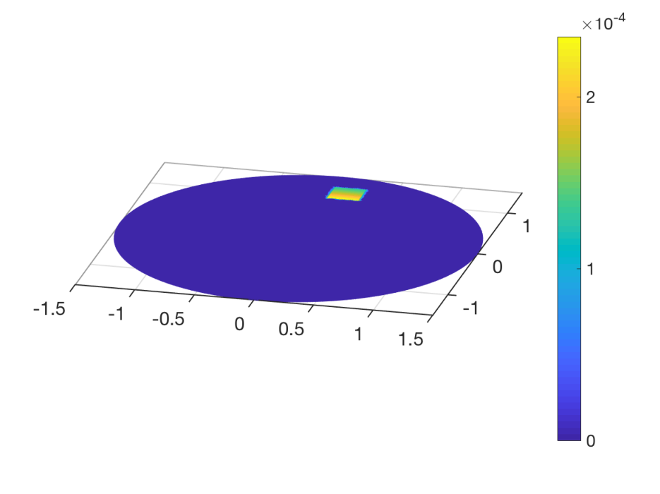
where the source is either ff (force or load) or zz (boundary control) see [6, 29, 36]. In (1.1) there is no provision to place the source in Ω^\widehat{\Omega} (cf. Figure 1). The issue is that the operator Δ\Delta has “lesser reach”, in other words, it is a local operator. On the other hand the fractional Laplacian (−Δ)s(-\Delta)^{s} with 0<s<10<s<1 (see (2.3)) is a nonlocal operator. This difference in behavior can be easily seen in our numerical examples in Section 7.2 where we observe that we cannot see the external source as ss approaches 1.

Recently, nonlocal diffusion operators such as the fractional Laplacian (−Δ)s(-\Delta)^{s} have emerged as an excellent alternative to model diffusion. Under a probabilistic framework this operator can be derived as a limit of the so-called long jump random walk [38]. Recall that Δ\Delta is the limit of the classical random walk or the Brownian motion. More applications of these models appear in (but not limited to) image denoising and phase field modeling [4]; image denosing where ss is allowed to be spatially dependent [10]; fractional diffusion maps (data analysis) [5]; magnetotellurics (geophysics) [44].

Coming back to the question of source/control placement, we next state the exterior value problem corresponding to (−Δ)s(-\Delta)^{s}. Find uu in an appropriate function space satisfying

(1.2) (−Δ)s​u=fin ​Ω,u=zon ​ℝN∖Ω.(-\Delta)^{s}u=f\quad\mbox{in }\Omega,\quad u=z\quad\mbox{on }{\mathbb{R}}^{N}\setminus\Omega.

As in the case of (1.1), besides ff being the source/control in Ω\Omega we can also place the source/control zz in the exterior domain ℝN∖Ω{\mathbb{R}}^{N}\setminus\Omega. However, the action of zz in (1.2) is significantly different from (1.1). Indeed, the source/control in (1.1) is placed on the boundary ∂Ω\partial\Omega, but the source/control zz in (1.2) is placed outside in ℝN∖Ω{\mathbb{R}}^{N}\setminus\Omega which is what we wanted to achieve in Figure 1. For completeness, we refer to [11] for the optimal control problem, with ff being the source/control and [12, 13] for another inverse problem to identify the coefficients in the fractional pp-Laplacian.

The purpose of this paper is to introduce and study a new class of the Dirichlet, Robin, and Neumann source identification problems or the optimal control problems. We shall use these terms interchangeably but we will make a distinction in our numerical experiments. We emphasize that yet another class of identification where the unknown is the fractional exponent ss for the spectral fractional Laplacian (which is different from the operator under consideration) was recently considered in [35]. We shall describe our problems next.

Let Ω⊂ℝN\Omega\subset{\mathbb{R}}^{N}, N≥1N\geq 1, be a bounded open set with boundary ∂Ω\partial\Omega. Let (ZD,UD)(Z_{D},U_{D}) and (ZR,UR)(Z_{R},U_{R}), where subscripts DD and RR indicate Dirichlet and Robin, be Banach spaces. The goal of this paper is to consider the following two external control or source identification problems. The source/control in our case is denoted by zz.

  • •

    Fractional Dirichlet exterior control problem: Given ξ≥0\xi\geq 0 a constant penalty parameter we consider the minimization problem:

    (1.3a) min(u,z)∈(UD,ZD)⁡J⁡(u)+ξ2​‖z‖ZD2,\min_{(u,z)\in(U_{D},Z_{D})}J(u)+\frac{\xi}{2}\|z\|^{2}_{Z_{D}},
    subject to the fractional Dirichlet exterior value problem: Find u∈UDu\in U_{D} solving
    (1.3b) {(−Δ)s​u=0in Ω,u=zin ℝN∖Ω,\begin{cases}(-\Delta)^{s}u&=0\quad\mbox{in }\Omega,\\ u&=z\quad\mbox{in }{\mathbb{R}}^{N}\setminus\Omega,\end{cases}
    and the control constraints
    (1.3c) z∈Za​d,D,z\in Z_{ad,D},

    with Za​d,D⊂ZDZ_{ad,D}\subset Z_{D} being a closed and convex subset.

  • •

    Fractional Robin exterior control problem: Given ξ≥0\xi\geq 0 a constant penalty parameter we consider the minimization problem

    (1.4a) min(u,z)∈(UR,ZR)⁡J⁡(u)+ξ2​‖z‖ZR2,\min_{(u,z)\in(U_{R},Z_{R})}J(u)+\frac{\xi}{2}\|z\|^{2}_{Z_{R}},
    subject to the fractional Robin exterior value problem: Find u∈URu\in U_{R} solving
    (1.4b) {(−Δ)s​u=0in Ω,𝒩s​u+κ​u=κzin ℝN∖Ω,\begin{cases}(-\Delta)^{s}u&=0\quad\mbox{in }\Omega,\\ \mathcal{N}_{s}u+\kappa u&=\kappa z\quad\mbox{in }{\mathbb{R}}^{N}\setminus\Omega,\end{cases}
    and the control constraints
    (1.4c) z∈Za​d,R,z\in Z_{ad,R},

    with Za​d,R⊂ZRZ_{ad,R}\subset Z_{R} being a closed and convex subset. In (1.4b), 𝒩s​u\mathcal{N}_{s}u is the nonlocal normal derivative of uu given in (2.4) below, κ∈L1​(ℝN∖Ω)∩L∞​(ℝN∖Ω)\kappa\in L^{1}(\mathbb{R}^{N}\setminus\Omega)\cap L^{\infty}(\mathbb{R}^{N}\setminus\Omega) and is non-negative. We notice that the latter assumption is not a restriction since otherwise we can replace κ\kappa throughout by |κ||\kappa|.

The precise conditions on Ω\Omega, JJ and the Banach spaces involved will be given in the subsequent sections. Notice that both the exterior value problems (1.3b) and (1.4b) are ill-posed if the conditions are enforced on ∂Ω\partial\Omega. The main difficulties in (1.3) and (1.4) stem from the following facts.

  1. ∙\bullet

    Nonlocal operator. The fractional Laplacian (−Δ)s(-\Delta)^{s} is a nonlocal operator. This can be easily seen from the definition of (−Δ)s(-\Delta)^{s} in (2.3).

  2. ∙\bullet

    Double nonlocality. The first order optimality conditions for (1.3) and the Robin exterior value problem (1.4b) require to study 𝒩s​u\mathcal{N}_{s}u which is the so-called nonlocal-normal derivative of uu (see (2.4)). Thus we not only have the nonlocal operator (−Δ)s(-\Delta)^{s} on the domain but also on the exterior ℝN∖Ω¯{\mathbb{R}}^{N}\setminus\overline{\Omega}, i.e., a double nonlocality.

  3. ∙\bullet

    Exterior conditions in ℝN∖Ω{\mathbb{R}}^{N}\setminus\Omega and not boundary conditions on ∂Ω\partial\Omega. The conditions in (1.3b) and (1.4b) need to be specified in ℝN∖Ω{\mathbb{R}}^{N}\setminus\Omega instead on ∂Ω\partial\Omega as otherwise the problems (1.3) and (1.4) are ill-posed as we have already mentioned above.

  4. ∙\bullet

    Very-weak solutions of nonlocal exterior value problems. A typical choice for ZZ is L2​(ℝN∖Ω)L^{2}({\mathbb{R}}^{N}\setminus\Omega). As a result, the Dirichlet exterior value problem (1.3b) can only have very-weak solutions (cf. [14, 15, 17] for the case s=1s=1). To the best of our knowledge this is the first work that considers the notion of very-weak solutions for nonlocal (fractional) exterior value problems associated with the fractional Laplace operator.

  5. ∙\bullet

    Regularity of optimization variables. The standard shift-theorem which holds for local operators such as Δ\Delta does not hold always hold for nonlocal operators such as (−Δ)s(-\Delta)^{s} (see for example [26]).

In view of all these aforementioned challenges it is clear that the standard techniques which are now well established for local problems do not directly extend to the nonlocal problems investigated in the present paper.

The purpose of this paper is to discuss our approach to deal with these nontrivial issues. We emphasize that to the best of our knowledge this is the first work that considers the optimal control of problems (source identification problems) (1.3b) and (1.4b) where the control/source is applied from the outside. Let us also mention that this notion of controllability of PDEs from the exterior has been introduced by M. Warma in [42] for the nonlocal heat equation associated with the fractional Laplacian and in [30] for the wave type equation with the fractional Laplace operator to study their controllability properties. The case of the strong damping wave equation is included in [43] where some controllability results have been obtained. In case of problems with the spectral fractional Laplacian the boundary control has been established in [9].

We mention that we can also deal with the fractional Neumann exterior control problem. That is, given ξ≥0\xi\geq 0 a constant penalty parameter,

min(u,z)∈(UN,ZN)⁡J⁡(u)+ξ2​‖z‖ZN2,\min_{(u,z)\in(U_{N},Z_{N})}J(u)+\frac{\xi}{2}\|z\|^{2}_{Z_{N}},

subject to the fractional Neumann exterior value problem: Find u∈UNu\in U_{N} solving

(1.5) {(−Δ)s​u+u=0in Ω,𝒩s​u=zin ℝN∖Ω,\begin{cases}(-\Delta)^{s}u+u&=0\quad\mbox{in }\Omega,\\ \mathcal{N}_{s}u&=z\quad\mbox{in }{\mathbb{R}}^{N}\setminus\Omega,\end{cases}

and the control constraints

z∈Za​d,N.z\in Z_{ad,N}.

The term uu is added in (1.5) just to ensure the uniqueness of solutions. The proofs follow similarly as the two cases we consider in the present paper with very minor changes. Since the paper is already long, we shall not give any details on this case.

Below we mention further the key-novelties of the present paper:

  1. (i)(i)

    For the first time, we introduce and study the notion of very-weak solutions to the Dirichlet exterior value problem (1.3b) which is suitable for optimal control problems. We also study weak solutions of the Robin exterior value problem (1.4b).

  2. (i​i)(ii)

    We approximate the weak solutions of nonhomogeneous Dirichlet exterior value problem by using a suitable Robin exterior value problem. This allows us to circumvent approximating the nonlocal normal derivative. This is a new approach to impose non-zero exterior conditions for the fractional Dirichlet exterior value problem. We refer to an alternative approach [3] where the authors use the Lagrange multipliers to impose nonzero Dirichlet exterior conditions.

  3. (i​i​i)(iii)

    We study both Dirichlet and Robin exterior control problems.

  4. (i​v)(iv)

    We approximate (with rate) the Dirichlet exterior control problem by a suitable Robin exterior control problem.

The rest of the paper is organized as follows. We begin with Section 2 where we introduce the relevant notations and function spaces. The material in this section is well-known. Our main work starts from Section 3 where at first we study the weak and very-weak solutions for the Dirichlet exterior value problem in Subsection 3.1. This is followed by the well-posedness of the Robin exterior value problem in Subsection 3.2. The Dirichlet exterior control problem is considered in Section 4 and Robin in Section 5. We show how to approximate the weak solutions to Dirichlet problem and the solutions to Dirichlet exterior control problem in Section 6. Subsection 7.1 is devoted to the experimental rate of convergence to approximate the Dirichlet exterior value problem using the Robin problem. In Subsection 7.2 we consider a source identification problem in the classical sense, however our source is located outside the observation domain where the PDE is satisfied. Subsection 7.3 is devoted to two optimal control problems.

Remark 1.1 (Practical aspects).

From a practical point of view, having the source/control over the entire ℝN∖Ω{\mathbb{R}}^{N}\setminus\Omega can be very expensive. But this can be easily fixed by appropriately describing Za​dZ_{ad}. Indeed in case of Figure 1 we can set the support of functions in Za​dZ_{ad} to be in Ω^∖Ω\widehat{\Omega}\setminus\Omega.

2. Notation and Preliminaries

Unless otherwise stated, Ω⊂ℝN\Omega\subset{\mathbb{R}}^{N} (N≥1N\geq 1) is a bounded open set and 0<s<10<s<1. We let

Ws,2(Ω):={u∈L2(Ω):∫Ω∫Ωu⁡(x)−u⁡(y)|x−y|N+2​sdxdy<∞},W^{s,2}(\Omega)\mathrel{\mathop{\mathchar 58\relax}}=\left\{u\in L^{2}(\Omega)\;\mathrel{\mathop{\mathchar 58\relax}}\;\int_{\Omega}\int_{\Omega}\frac{u(x)-u(y)}{|x-y|^{N+2s}}\;dxdy<\infty\right\},

and we endow it with the norm defined by

‖u‖Ws,2​(Ω):=(∫Ω|u|2​𝑑x+∫Ω∫Ω|u⁡(x)−u⁡(y)|2|x−y|N+2​s​𝑑x​𝑑y)12.\|u\|_{W^{s,2}(\Omega)}\mathrel{\mathop{\mathchar 58\relax}}=\left(\int_{\Omega}|u|^{2}\;dx+\int_{\Omega}\int_{\Omega}\frac{|u(x)-u(y)|^{2}}{|x-y|^{N+2s}}\;dxdy\right)^{\frac{1}{2}}.

In order to study (1.3b) we also need to define

W0s,2(Ω¯):={u∈Ws,2(ℝN):u=0 in ℝN∖Ω}.W^{s,2}_{0}(\overline{\Omega})\mathrel{\mathop{\mathchar 58\relax}}=\left\{u\in W^{s,2}({\mathbb{R}}^{N})\;\mathrel{\mathop{\mathchar 58\relax}}\;u=0\mbox{ in }{\mathbb{R}}^{N}\setminus\Omega\right\}.

Then

‖u‖W0s,2​(Ω¯):=(∫ℝN∫ℝN|u⁡(x)−u⁡(y)|2|x−y|N+2​s​𝑑x​𝑑y)12\displaystyle\|u\|_{W_{0}^{s,2}(\overline{\Omega})}\mathrel{\mathop{\mathchar 58\relax}}=\left(\int_{{\mathbb{R}}^{N}}\int_{{\mathbb{R}}^{N}}\frac{|u(x)-u(y)|^{2}}{|x-y|^{N+2s}}\;dxdy\right)^{\frac{1}{2}}

defines an equivalent norm on W0s,2​(Ω¯)W_{0}^{s,2}(\overline{\Omega}).

We shall use W−s,2​(ℝN)W^{-s,2}({\mathbb{R}}^{N}) and W−s,2​(Ω¯)W^{-s,2}(\overline{\Omega}) to denote the dual spaces of Ws,2​(ℝN)W^{s,2}({\mathbb{R}}^{N}) and W0s,2​(Ω¯)W_{0}^{s,2}(\overline{\Omega}), respectively, and ⟨⋅,⋅⟩\langle\cdot,\cdot\rangle, to denote their duality pairing whenever it is clear from the context.

We also define the local fractional order Sobolev space

(2.1) Wlocs,2(ℝN∖Ω):={u∈L2(ℝN∖Ω):uφ∈Ws,2(ℝN∖Ω),∀φ∈𝒟(ℝN∖Ω)}.W^{s,2}_{\rm loc}(\mathbb{R}^{N}\setminus\Omega)\mathrel{\mathop{\mathchar 58\relax}}=\left\{u\in L^{2}(\mathbb{R}^{N}\setminus\Omega)\;\mathrel{\mathop{\mathchar 58\relax}}\;u\varphi\in W^{s,2}(\mathbb{R}^{N}\setminus\Omega),\ \forall\ \varphi\in\mathcal{D}(\mathbb{R}^{N}\setminus\Omega)\right\}.

To introduce the fractional Laplace operator, we let 0<s<10<s<1, and we set

𝕃s1(ℝN):={u:ℝN→ℝ measurable, ∫ℝN|u⁡(x)|(1+|x|)N+2​sdx<∞}.\mathbb{L}_{s}^{1}({\mathbb{R}}^{N})\mathrel{\mathop{\mathchar 58\relax}}=\left\{u\mathrel{\mathop{\mathchar 58\relax}}{\mathbb{R}}^{N}\rightarrow\mathbb{R}\;\mbox{ measurable, }\;\int_{{\mathbb{R}}^{N}}\frac{|u(x)|}{(1+|x|)^{N+2s}}\;dx<\infty\right\}.

For u∈𝕃s1​(ℝN)u\in\mathbb{L}_{s}^{1}({\mathbb{R}}^{N}) and ε>0\varepsilon>0, we let

(−Δ)εs​u​(x)=CN,s​∫{y∈ℝN,|y−x|>ε}u⁡(x)−u⁡(y)|x−y|N+2​s​𝑑y,x∈ℝN,(-\Delta)_{\varepsilon}^{s}u(x)=C_{N,s}\int_{\{y\in{\mathbb{R}}^{N},|y-x|>\varepsilon\}}\frac{u(x)-u(y)}{|x-y|^{N+2s}}dy,\;\;x\in{\mathbb{R}}^{N},

where the normalized constant CN,sC_{N,s} is given by

(2.2) CN,s:=s​22​s​Γ​(2​s+N2)πN2​Γ​(1−s),C_{N,s}\mathrel{\mathop{\mathchar 58\relax}}=\frac{s2^{2s}\Gamma\left(\frac{2s+N}{2}\right)}{\pi^{\frac{N}{2}}\Gamma(1-s)},

and Γ\Gamma is the usual Euler Gamma function (see, e.g. [18, 20, 21, 22, 23, 40, 41]). The fractional Laplacian (−Δ)s(-\Delta)^{s} is defined for u∈𝕃s1​(ℝN)u\in\mathbb{L}_{s}^{1}({\mathbb{R}}^{N}) by the formula

(2.3) (−Δ)s​u​(x)=CN,s​P.V.​∫ℝNu⁡(x)−u⁡(y)|x−y|N+2​s​𝑑y=limε↓0(−Δ)εs​u​(x),x∈ℝN,\displaystyle(-\Delta)^{s}u(x)=C_{N,s}\mbox{P.V.}\int_{{\mathbb{R}}^{N}}\frac{u(x)-u(y)}{|x-y|^{N+2s}}dy=\lim_{\varepsilon\downarrow 0}(-\Delta)_{\varepsilon}^{s}u(x),\;\;x\in{\mathbb{R}}^{N},

provided that the limit exists. It has been shown in [19, Proposition 2.2] that for u∈𝒟⁡(Ω)u\in\mathcal{D}(\Omega), we have that

lims↑1∫ℝNu(−Δ)sudx=∫ℝN|∇u|2dx=−∫ℝNuΔudx=−∫ΩuΔudx,\lim_{s\uparrow 1}\int_{{\mathbb{R}}^{N}}u(-\Delta)^{s}u\;dx=\int_{{\mathbb{R}}^{N}}|\nabla u|^{2}dx=-\int_{{\mathbb{R}}^{N}}u\Delta u\;dx=-\int_{\Omega}u\Delta u\;dx,

that is where the constant CN,sC_{N,s} plays a crucial role.

Next, for u∈Ws,2​(ℝN)u\in W^{s,2}({\mathbb{R}}^{N}) we define the nonlocal normal derivative 𝒩s\mathcal{N}_{s} as:

(2.4) 𝒩s​u​(x):=CN,s​∫Ωu⁡(x)−u⁡(y)|x−y|N+2​s​𝑑y,x∈ℝN∖Ω¯.\displaystyle\mathcal{N}_{s}u(x)\mathrel{\mathop{\mathchar 58\relax}}=C_{N,s}\int_{\Omega}\frac{u(x)-u(y)}{|x-y|^{N+2s}}\;dy,\quad x\in{\mathbb{R}}^{N}\setminus\overline{\Omega}.

We shall call 𝒩s\mathcal{N}_{s} the interaction operator. Clearly 𝒩s\mathcal{N}_{s} is a nonlocal operator and it is well defined on Ws,2​(ℝN)W^{s,2}({\mathbb{R}}^{N}) as we discuss next.

Lemma 2.1.

The interaction operator 𝒩s\mathcal{N}_{s} maps continuously Ws,2​(ℝN)W^{s,2}({\mathbb{R}}^{N}) into Wlocs,2​(ℝN∖Ω)W^{s,2}_{\rm loc}({\mathbb{R}}^{N}\setminus\Omega). As a result, if u∈Ws,2​(ℝN)u\in W^{s,2}({\mathbb{R}}^{N}), then 𝒩s​u∈L2​(ℝN∖Ω)\mathcal{N}_{s}u\in L^{2}({\mathbb{R}}^{N}\setminus\Omega).

Proof.

We refer to [25, Lemma 3.2] for the proof of the first part. The second part is a direct consequence of (2.1). ∎

Despite the fact that 𝒩s\mathcal{N}_{s} is defined on ℝN∖Ω{\mathbb{R}}^{N}\setminus\Omega, it is still known as the “normal” derivative. This is due to its similarity with the classical normal derivative as we shall discuss next.

Proposition 2.2.

The following assertions hold.

  1. (a)

    The divergence theorem for (−Δ)s(-\Delta)^{s}. Let u∈C02​(ℝN)u\in C_{0}^{2}({\mathbb{R}}^{N}), i.e., C2C^{2} functions on ℝN{\mathbb{R}}^{N} that vanishes at ±∞\pm\infty. Then

    ∫Ω(−Δ)sudx=−∫ℝN∖Ω𝒩sudx.\int_{\Omega}(-\Delta)^{s}u\;dx=-\int_{{\mathbb{R}}^{N}\setminus\Omega}\mathcal{N}_{s}u\;dx.
  2. (b)

    The integration by parts formula for (−Δ)s(-\Delta)^{s}. Let u∈Ws,2​(ℝN)u\in W^{s,2}({\mathbb{R}}^{N}) be such that (−Δ)s​u∈L2​(Ω)(-\Delta)^{s}u\in L^{2}(\Omega). Then for every v∈Ws,2​(ℝN)v\in W^{s,2}({\mathbb{R}}^{N}) we have that

    CN,s2∫∫ℝ2​N∖(ℝN∖Ω)2\displaystyle\frac{C_{N,s}}{2}\int\int_{{\mathbb{R}}^{2N}\setminus({\mathbb{R}}^{N}\setminus\Omega)^{2}} (u⁡(x)−u⁡(y))​(v⁡(x)−v⁡(y))|x−y|N+2​s​d​x​d​y\displaystyle\frac{(u(x)-u(y))(v(x)-v(y))}{|x-y|^{N+2s}}\;dxdy
    (2.5) =∫Ωv​(−Δ)s​u​𝑑x+∫ℝN∖Ωv​𝒩s​u​𝑑x,\displaystyle=\int_{\Omega}v(-\Delta)^{s}u\;dx+\int_{{\mathbb{R}}^{N}\setminus\Omega}v\mathcal{N}_{s}u\;dx,

    where ℝ2​N∖(ℝN∖Ω)2:=(Ω×Ω)∪(Ω×(ℝN∖Ω))∪((ℝN∖Ω)×Ω){\mathbb{R}}^{2N}\setminus({\mathbb{R}}^{N}\setminus\Omega)^{2}\mathrel{\mathop{\mathchar 58\relax}}=(\Omega\times\Omega)\cup(\Omega\times({\mathbb{R}}^{N}\setminus\Omega))\cup(({\mathbb{R}}^{N}\setminus\Omega)\times\Omega).

  3. (c)

    The limit as s↑1s\uparrow 1. Let u,v∈C02​(ℝN)u,v\in C_{0}^{2}({\mathbb{R}}^{N}). Then

    lims↑1∫ℝN∖Ωv​𝒩s​u​𝑑x=∫∂Ω∂u∂ν​v​𝑑σ.\lim_{s\uparrow 1}\int_{{\mathbb{R}}^{N}\setminus\Omega}v\mathcal{N}_{s}u\;dx=\int_{\partial\Omega}\frac{\partial u}{\partial\nu}vd\sigma.
Remark 2.3.

Comparing (a)-(c) in Proposition 2.2 with the classical properties of the standard Laplacian Δ\Delta we can immediately infer that 𝒩s\mathcal{N}_{s} plays the same role for (−Δ)s(-\Delta)^{s} that the classical normal derivative does for Δ\Delta. For this reason, we call 𝒩s\mathcal{N}_{s} the nonlocal normal derivative.

Proof of Proposition 2.2.

The proofs of Parts (a) and (c) are contained in [24, Lemma 3.2] and [24, Proposition 5.1], respectively. The proof of Part (b) for smooth functions can be found in [24, Lemma 3.3]. The version given here is obtained by using a density argument (cf. [42, Proposition 3.7]). ∎

3. The state equations

Before analyzing the optimal control problems (1.3) and (1.4), for a given function zz we shall focus on the Dirichlet (1.3b) and Robin (1.4b) exterior value problems. We shall assume that Ω\Omega is a bounded domain with Lipschitz continuous boundary.

3.1. The Dirichlet problem for the fractional Laplacian

We begin by rewriting the system (1.3b) in a more general form

(3.1) {(−Δ)s​u=fin ​Ω,u=zin ​ℝN∖Ω.\begin{cases}(-\Delta)^{s}u=f\quad&\mbox{in }\Omega,\\ u=z\quad&\mbox{in }{\mathbb{R}}^{N}\setminus\Omega.\end{cases}

Here is our notion of weak solutions.

Definition 3.1 (Weak solution to the Dirichlet problem).

Let f∈W−s,2​(Ω¯)f\in W^{-s,2}(\overline{\Omega}), z∈Ws,2​(ℝN∖Ω)z\in W^{s,2}({\mathbb{R}}^{N}\setminus\Omega) and 𝒵∈Ws,2​(ℝN)\mathcal{Z}\in W^{s,2}({\mathbb{R}}^{N}) be such that 𝒵|ℝN∖Ω=z\mathcal{Z}|_{{\mathbb{R}}^{N}\setminus\Omega}=z. A u∈Ws,2​(ℝN)u\in W^{s,2}({\mathbb{R}}^{N}) is said to be a weak solution to (3.1) if u−𝒵∈W0s,2​(Ω¯)u-\mathcal{Z}\in W^{s,2}_{0}(\overline{\Omega}) and

CN,s2​∫ℝN∫ℝN(u⁡(x)−u⁡(y))​(v⁡(x)−v⁡(y))|x−y|N+2​s​𝑑x​𝑑y=⟨f,v⟩,\frac{C_{N,s}}{2}\int_{{\mathbb{R}}^{N}}\int_{{\mathbb{R}}^{N}}\frac{(u(x)-u(y))(v(x)-v(y))}{|x-y|^{N+2s}}\;dxdy=\langle f,v\rangle,

for every v∈W0s,2​(Ω¯)v\in W^{s,2}_{0}(\overline{\Omega}).

Firstly, we notice that since Ω\Omega is assumed to have a Lipschitz continuous boundary, we have that, for z∈Ws,2​(ℝN∖Ω)z\in W^{s,2}(\mathbb{R}^{N}\setminus\Omega), there exists 𝒵∈Ws,2​(ℝN)\mathcal{Z}\in W^{s,2}({\mathbb{R}}^{N}) such that 𝒵|ℝN∖Ω=z\mathcal{Z}|_{\mathbb{R}^{N}\setminus\Omega}=z. Secondly, the existence and uniqueness of a weak solution uu to (3.1) and the continuous dependence of uu on the data ff and zz have been considered in [27], see also [25, 39]. More precisely we have the following result.

Proposition 3.2.

Let f∈W−s,2​(Ω¯)f\in W^{-s,2}(\overline{\Omega}) and z∈Ws,2​(ℝN∖Ω)z\in W^{s,2}({\mathbb{R}}^{N}\setminus\Omega). Then there exists a unique weak solution uu to (3.1) in the sense of Definition 3.1. In addition there is a constant C>0C>0 such that

(3.2) ‖u‖Ws,2​(ℝN)≤C⁡(‖f‖W−s,2​(Ω¯)+‖z‖Ws,2​(ℝN∖Ω)).\displaystyle\|u\|_{W^{s,2}({\mathbb{R}}^{N})}\leq C\left(\|f\|_{W^{-s,2}(\overline{\Omega})}+\|z\|_{W^{s,2}({\mathbb{R}}^{N}\setminus\Omega)}\right).

Even though such a result is typically sufficient in most situations, nevertheless it is not directly useful in the current context of optimal control problem (1.3) since we are interested in taking the space ZD=L2​(ℝN∖Ω)Z_{D}=L^{2}({\mathbb{R}}^{N}\setminus\Omega). Thus we need existence of solution (in some sense) to the fractional Dirichlet problem (3.1) when the datum z∈L2​(ℝN∖Ω)z\in L^{2}({\mathbb{R}}^{N}\setminus\Omega). In order to tackle this situation we introduce the notion of very-weak solutions for (3.1).

Definition 3.3 (Very-weak solution to the Dirichlet problem).

Let z∈L2​(ℝN∖Ω)z\in L^{2}({\mathbb{R}}^{N}\setminus\Omega) and f∈W−s,2​(Ω¯)f\in W^{-s,2}(\overline{\Omega}). A u∈L2​(ℝN)u\in L^{2}({\mathbb{R}}^{N}) is said to be a very-weak solution to (3.1) if the identity

(3.3) ∫Ωu​(−Δ)s​v​𝑑x=⟨f,v⟩−∫ℝN∖Ωz​𝒩s​v​𝑑x,\int_{\Omega}u(-\Delta)^{s}v\;dx=\langle f,v\rangle-\int_{{\mathbb{R}}^{N}\setminus\Omega}z\mathcal{N}_{s}v\;dx,

holds for every v∈V:={v∈W0s,2(Ω¯):(−Δ)sv∈L2(Ω)}v\in V\mathrel{\mathop{\mathchar 58\relax}}=\{v\in W^{s,2}_{0}(\overline{\Omega})\;\mathrel{\mathop{\mathchar 58\relax}}\;(-\Delta)^{s}v\in L^{2}(\Omega)\}.

Next we prove the existence and uniqueness of a very-weak solution to (3.1) in the sense of Definition 3.3.

Theorem 3.4.

Let f∈W−s,2​(Ω¯)f\in W^{-s,2}(\overline{\Omega}) and z∈L2​(ℝN∖Ω)z\in L^{2}({\mathbb{R}}^{N}\setminus\Omega). Then there exists a unique very-weak solution uu to (3.1) according to Definition 3.1 that fulfills

(3.4) ‖u‖L2​(Ω)≤C⁡(‖f‖W−s,2​(Ω¯)+‖z‖L2​(ℝN∖Ω)),\displaystyle\|u\|_{L^{2}(\Omega)}\leq C\left(\|f\|_{W^{-s,2}(\overline{\Omega})}+\|z\|_{L^{2}({\mathbb{R}}^{N}\setminus\Omega)}\right),

for a constant C>0C>0. In addition, if z∈Ws,2​(ℝN∖Ω)z\in W^{s,2}(\mathbb{R}^{N}\setminus\Omega), then the following assertions hold.

  1. (a)

    Every weak solution of (3.1) is also a very-weak solution.

  2. (b)

    Every very-weak solution of (3.1) that belongs to Ws,2​(ℝN)W^{s,2}({\mathbb{R}}^{N}) is also a weak solution.

Proof.

In order to show the existence of a very-weak solution we shall apply the Babuška-Lax-Milgram theorem.

Firstly, let (−Δ)Ds(-\Delta)_{D}^{s} be the realization of (−Δ)s(-\Delta)^{s} in L2​(Ω)L^{2}(\Omega) with the zero Dirichlet exterior condition u=0u=0 in ℝN∖Ω{\mathbb{R}}^{N}\setminus\Omega. More precisely,

D⁡((−Δ)Ds)=V​ and ​(−Δ)Ds​u=(−Δ)s​u.\displaystyle D((-\Delta)_{D}^{s})=V\;\mbox{ and }\;(-\Delta)_{D}^{s}u=(-\Delta)^{s}u.

Then a norm on VV is given by ‖v‖V=‖(−Δ)Ds​v‖L2​(Ω)\|v\|_{V}=\|(-\Delta)_{D}^{s}v\|_{L^{2}(\Omega)} which follows from the fact that the operator (−Δ)Ds(-\Delta)_{D}^{s} is invertible (since by [34] (−Δ)Ds(-\Delta)_{D}^{s} has a compact resolvent and its first eigenvalue is strictly positive). Secondly, let ℱ\mathcal{F} be the bilinear form defined on L2​(Ω)×VL^{2}(\Omega)\times V by

ℱ⁡(u,v):=∫Ωu​(−Δ)s​v​𝑑x.\displaystyle\mathcal{F}(u,v)\mathrel{\mathop{\mathchar 58\relax}}=\int_{\Omega}u(-\Delta)^{s}v\;dx.

Then ℱ\mathcal{F} is clearly bounded on L2​(Ω)×VL^{2}(\Omega)\times V. More precisely there is a constant C>0C>0 such that

|ℱ⁡(u,v)|≤‖u‖L2​(Ω)​‖(−Δ)s​v‖L2​(ΩCLOSE≤C​‖u‖L2​(Ω)​‖v‖V.\displaystyle\left|\mathcal{F}(u,v)\right|\leq\|u\|_{L^{2}(\Omega)}\|(-\Delta)^{s}v\|_{L^{2}(\Omega}\leq C\|u\|_{L^{2}(\Omega)}\|v\|_{V}.

Thirdly, we show the inf-sup conditions. From the definition of VV, it immediately follows that

v∈W0s,2(Ω¯) and (−Δ)sv∈L2(Ω)⟺v∈V.\displaystyle v\in W_{0}^{s,2}(\overline{\Omega})\;\;\mbox{ and }\;(-\Delta)^{s}v\in L^{2}(\Omega)\quad\Longleftrightarrow\quad v\in V.

By setting u:=(−Δ)Ds​v‖(−Δ)Ds​v‖L2​(Ω)∈L2​(Ω)u\mathrel{\mathop{\mathchar 58\relax}}=\frac{(-\Delta)_{D}^{s}v}{\|(-\Delta)_{D}^{s}v\|_{L^{2}(\Omega)}}\in L^{2}(\Omega), we obtain that

supu∈L2​(Ω),‖u‖L2​(Ω)=1|(u,(−Δ)Ds​v)L2​(Ω)|\displaystyle\sup_{u\in L^{2}(\Omega),\|u\|_{L^{2}(\Omega)}=1}|(u,(-\Delta)_{D}^{s}v)_{L^{2}(\Omega)}| ≥|((−Δ)Ds​v,(−Δ)Ds​v)L2​(Ω)|‖(−Δ)Ds​v‖L2​(Ω)\displaystyle\geq\frac{|((-\Delta)_{D}^{s}v,(-\Delta)_{D}^{s}v)_{L^{2}(\Omega)}|}{\|(-\Delta)_{D}^{s}v\|_{L^{2}(\Omega)}}
=‖(−Δ)Ds​v‖L2​(Ω)=‖v‖V.\displaystyle=\|(-\Delta)_{D}^{s}v\|_{L^{2}(\Omega)}=\|v\|_{V}.

Next we choose v∈Vv\in V as the unique weak solution of (−Δ)Ds​v=u/‖u‖L2​(Ω)(-\Delta)_{D}^{s}v=u/\|u\|_{L^{2}(\Omega)} for some 0≠u∈L2​(Ω)0\neq u\in L^{2}(\Omega). Then we readily obtain that

supv∈V,‖v‖V=1|(u,(−Δ)s​v)L2​(Ω)|≥|(u,u)L2​(Ω)|‖u‖L2​(Ω)=‖u‖L2​(Ω)>0,\sup_{v\in V,\|v\|_{V}=1}|(u,(-\Delta)^{s}v)_{L^{2}(\Omega)}|\geq\frac{|(u,u)_{L^{2}(\Omega)}|}{\|u\|_{L^{2}(\Omega)}}=\|u\|_{L^{2}(\Omega)}>0,

for all 0≠u∈L2​(Ω)0\neq u\in L^{2}(\Omega). Finally, we have to show that the right-hand-side in (3.3) defines a linear continuous functional on VV. Indeed, applying the Hölder inequality in conjunction with Lemma 2.1 we obtain that there is a constant C>0C>0 such that

(3.5) |∫ℝN∖Ωz​𝒩s​v​𝑑x|≤‖z‖L2​(ℝN∖Ω)​‖𝒩s​v‖L2​(ℝN∖Ω)≤C​‖z‖L2​(ℝN∖Ω)​‖v‖W0s,2​(Ω¯),\displaystyle\left|\int_{{\mathbb{R}}^{N}\setminus\Omega}z\mathcal{N}_{s}v\;dx\right|\leq\|z\|_{L^{2}({\mathbb{R}}^{N}\setminus\Omega)}\|\mathcal{N}_{s}v\|_{L^{2}({\mathbb{R}}^{N}\setminus\Omega)}\leq C\|z\|_{L^{2}({\mathbb{R}}^{N}\setminus\Omega)}\|v\|_{W^{s,2}_{0}(\overline{\Omega})},

where in the last step we have used the fact that ‖v‖W0s,2​(Ω¯)=‖v‖Ws,2​(ℝN)\|v\|_{W_{0}^{s,2}(\overline{\Omega})}=\|v\|_{W^{s,2}({\mathbb{R}}^{N})} for v∈W0s,2​(Ω¯)v\in W_{0}^{s,2}(\overline{\Omega}). Moreover

|⟨f,v⟩|≤‖f‖W−s,2​(Ω¯)​‖v‖W0s,2​(Ω¯).|\langle f,v\rangle|\leq\|f\|_{W^{-s,2}(\overline{\Omega})}\|v\|_{W^{s,2}_{0}(\overline{\Omega})}.

In view of the last two estimates, the right-hand-side in (3.3) defines a linear continuous functional on VV. Therefore all the requirements of the Babuška-Lax-Milgram theorem holds. Thus, there exists a unique u∈L2​(Ω)u\in L^{2}(\Omega) satisfying (3.3). Let u=zu=z in ℝN∖Ω\mathbb{R}^{N}\setminus\Omega, then u∈L2​(ℝN)u\in L^{2}({\mathbb{R}}^{N}) and satisfies (3.3). We have shown the existence of the uniqueness of a very-weak solution..

Next we show the estimate (3.4). Let u∈L2​(ℝN)u\in L^{2}({\mathbb{R}}^{N}) be a very-weak solution. Let v∈Vv\in V be a solution of (−Δ)Ds​v=u(-\Delta)_{D}^{s}v=u. Taking this vv as a test function in (3.3) and using (3.5), we get that there is a constant C>0C>0 such that

‖u‖L2​(Ω)2≤\displaystyle\|u\|_{L^{2}(\Omega)}^{2}\leq ‖f‖W−s,2​(Ω¯)​‖v‖W0s,2​(Ω¯)+‖z‖L2​(ℝN∖Ω)​‖𝒩s​v‖L2​(ℝN∖Ω)\displaystyle\|f\|_{W^{-s,2}(\overline{\Omega})}\|v\|_{W_{0}^{s,2}(\overline{\Omega})}+\|z\|_{L^{2}(\mathbb{R}^{N}\setminus\Omega)}\|\mathcal{N}_{s}v\|_{L^{2}(\mathbb{R}^{N}\setminus\Omega)}
≤\displaystyle\leq C⁡(‖f‖W−s,2​(Ω¯)+‖z‖L2​(ℝN∖Ω))​‖v‖W0s,2​(Ω¯)\displaystyle C\left(\|f\|_{W^{-s,2}(\overline{\Omega})}+\|z\|_{L^{2}(\mathbb{R}^{N}\setminus\Omega)}\right)\|v\|_{W_{0}^{s,2}(\overline{\Omega})}
≤\displaystyle\leq C⁡(‖f‖W−s,2​(Ω¯)+‖z‖L2​(ℝN∖Ω))​‖(−Δ)Ds​v‖L2​(Ω)\displaystyle C\left(\|f\|_{W^{-s,2}(\overline{\Omega})}+\|z\|_{L^{2}(\mathbb{R}^{N}\setminus\Omega)}\right)\|(-\Delta)_{D}^{s}v\|_{L^{2}(\Omega)}
≤\displaystyle\leq C⁡(‖f‖W−s,2​(Ω¯)+‖z‖L2​(ℝN∖Ω))​‖u‖L2​(Ω),\displaystyle C\left(\|f\|_{W^{-s,2}(\overline{\Omega})}+\|z\|_{L^{2}(\mathbb{R}^{N}\setminus\Omega)}\right)\|u\|_{L^{2}(\Omega)},

and we have shown (3.4). This completes the proof of the first part.

Next we prove the last two assertions of the theorem. Assume that z∈Ws,2​(ℝN∖Ω)z\in W^{s,2}(\mathbb{R}^{N}\setminus\Omega).

(a) Let u∈Ws,2​(ℝN)↪L2​(ℝN)u\in W^{s,2}({\mathbb{R}}^{N})\hookrightarrow L^{2}({\mathbb{R}}^{N}) be a weak solution of (3.1). It follows from the definition that u=zu=z in ℝN∖Ω{\mathbb{R}}^{N}\setminus\Omega and

(3.6) CN,s2​∫ℝN∫ℝN(u⁡(x)−u⁡(y))​(v⁡(x)−v⁡(y))|x−y|N+2​s​𝑑x​𝑑y=⟨f,v⟩,\displaystyle\frac{C_{N,s}}{2}\int_{{\mathbb{R}}^{N}}\int_{{\mathbb{R}}^{N}}\frac{(u(x)-u(y))(v(x)-v(y))}{|x-y|^{N+2s}}\;dxdy=\langle f,v\rangle,

for every v∈Vv\in V. Since v=0v=0 in ℝN∖Ω{\mathbb{R}}^{N}\setminus\Omega, we have that

∫ℝN∫ℝN\displaystyle\int_{{\mathbb{R}}^{N}}\int_{{\mathbb{R}}^{N}} (u⁡(x)−u⁡(y))​(v⁡(x)−v⁡(y))|x−y|N+2​s​d​x​d​y\displaystyle\frac{(u(x)-u(y))(v(x)-v(y))}{|x-y|^{N+2s}}\;dxdy
(3.7) =∫∫ℝ2​N∖(ℝN∖Ω)2(u⁡(x)−u⁡(y))​(v⁡(x)−v⁡(y))|x−y|N+2​s​𝑑x​𝑑y.\displaystyle=\int\int_{{\mathbb{R}}^{2N}\setminus({\mathbb{R}}^{N}\setminus\Omega)^{2}}\frac{(u(x)-u(y))(v(x)-v(y))}{|x-y|^{N+2s}}\;dxdy.

Using (3.6), (3.1), the integration by parts formula (2) together with the fact that u=zu=z in ℝN∖Ω{\mathbb{R}}^{N}\setminus\Omega, we get that

CN,s2∫ℝN∫ℝN\displaystyle\frac{C_{N,s}}{2}\int_{{\mathbb{R}}^{N}}\int_{{\mathbb{R}}^{N}} (u⁡(x)−u⁡(y))​(v⁡(x)−v⁡(y))|x−y|N+2​s​d​x​d​y\displaystyle\frac{(u(x)-u(y))(v(x)-v(y))}{|x-y|^{N+2s}}\;dxdy
=⟨f,v⟩\displaystyle=\langle f,v\rangle
=∫Ωu​(−Δ)s​v​𝑑x+∫ℝN∖Ωu​𝒩s​v​𝑑x\displaystyle=\int_{\Omega}u(-\Delta)^{s}v\;dx+\int_{{\mathbb{R}}^{N}\setminus\Omega}u\mathcal{N}_{s}v\;dx
=∫Ωu​(−Δ)s​v​𝑑x+∫ℝN∖Ωz​𝒩s​v​𝑑x.\displaystyle=\int_{\Omega}u(-\Delta)^{s}v\;dx+\int_{{\mathbb{R}}^{N}\setminus\Omega}z\mathcal{N}_{s}v\;dx.

Thus uu is a very-weak solution of (3.1).

(b) Finally let uu be a very-weak solution of (3.1) and assume that u∈Ws,2​(ℝN)u\in W^{s,2}({\mathbb{R}}^{N}). Since u=zu=z in ℝN∖Ω{\mathbb{R}}^{N}\setminus\Omega, we have that z∈Ws,2​(ℝN∖Ω)z\in W^{s,2}({\mathbb{R}}^{N}\setminus\Omega) and if 𝒵∈Ws,2​(ℝN)\mathcal{Z}\in W^{s,2}({\mathbb{R}}^{N}) satisfies 𝒵|ℝN∖Ω=z\mathcal{Z}|_{{\mathbb{R}}^{N}\setminus\Omega}=z, then clearly (u−𝒵)∈W0s,2​(Ω¯)(u-\mathcal{Z})\in W_{0}^{s,2}(\overline{\Omega}). Since uu is a very-weak solution of (3.1), then by definition, for every v∈V=D⁡((−Δ)Ds)v\in V=D((-\Delta)_{D}^{s}), we have that

(3.8) ∫Ωu​(−Δ)s​v​𝑑x=⟨f,v⟩−∫ℝN∖Ωz​𝒩s​v​𝑑x.\displaystyle\int_{\Omega}u(-\Delta)^{s}v\;dx=\langle f,v\rangle-\int_{{\mathbb{R}}^{N}\setminus\Omega}z\mathcal{N}_{s}v\;dx.

Since u∈Ws,2​(ℝN)u\in W^{s,2}({\mathbb{R}}^{N}) and v=0v=0 in ℝN∖Ω{\mathbb{R}}^{N}\setminus\Omega, then using (2) again we get that

∫ℝN∫ℝN\displaystyle\int_{{\mathbb{R}}^{N}}\int_{{\mathbb{R}}^{N}} (u⁡(x)−u⁡(y))​(v⁡(x)−v⁡(y))|x−y|N+2​s​d​x​d​y\displaystyle\frac{(u(x)-u(y))(v(x)-v(y))}{|x-y|^{N+2s}}\;dxdy
=∫∫ℝ2​N∖(ℝN∖Ω)2(u⁡(x)−u⁡(y))​(v⁡(x)−v⁡(y))|x−y|N+2​s​𝑑x​𝑑y\displaystyle=\int\int_{{\mathbb{R}}^{2N}\setminus({\mathbb{R}}^{N}\setminus\Omega)^{2}}\frac{(u(x)-u(y))(v(x)-v(y))}{|x-y|^{N+2s}}\;dxdy
=∫Ωu​(−Δ)s​v​𝑑x+∫ℝN∖Ωu​𝒩s​v​𝑑x\displaystyle=\int_{\Omega}u(-\Delta)^{s}v\;dx+\int_{{\mathbb{R}}^{N}\setminus\Omega}u\mathcal{N}_{s}v\;dx
(3.9) =∫Ωu​(−Δ)s​v​𝑑x+∫ℝN∖Ωz​𝒩s​v​𝑑x.\displaystyle=\int_{\Omega}u(-\Delta)^{s}v\;dx+\int_{{\mathbb{R}}^{N}\setminus\Omega}z\mathcal{N}_{s}v\;dx.

It follows from (3.8) and (3.1) that for every v∈Vv\in V, we have that

(3.10) ∫ℝN∫ℝN\displaystyle\int_{{\mathbb{R}}^{N}}\int_{{\mathbb{R}}^{N}} (u⁡(x)−u⁡(y))​(v⁡(x)−v⁡(y))|x−y|N+2​s​d​x​d​y=⟨f,v⟩.\displaystyle\frac{(u(x)-u(y))(v(x)-v(y))}{|x-y|^{N+2s}}\;dxdy=\langle f,v\rangle.

Since VV is dense in W0s,2​(Ω¯)W_{0}^{s,2}(\overline{\Omega}), we have that (3.10) remains true for every v∈W0s,2​(Ω¯)v\in W_{0}^{s,2}(\overline{\Omega}). We have shown that uu is a weak solution of (3.1) and the proof is finished. ∎

3.2. The Robin problem for the fractional Laplacian

In order to study the Robin problem (1.4b) we consider the Sobolev space introduced in [24]. For g∈L1​(ℝN∖Ω)g\in L^{1}({\mathbb{R}}^{N}\setminus\Omega) fixed, we let

WΩ,gs,2:={u:ℝN→ℝ measurable, ∥u∥WΩ,gs,2<∞},\displaystyle W_{\Omega,g}^{s,2}\mathrel{\mathop{\mathchar 58\relax}}=\Big\{u\mathrel{\mathop{\mathchar 58\relax}}{\mathbb{R}}^{N}\to{\mathbb{R}}\;\mbox{ measurable, }\,\|u\|_{W_{\Omega,g}^{s,2}}<\infty\Big\},

where

(3.11) ‖u‖WΩ,gs,2:=(‖u‖L2​(Ω)2+‖|g|12​u‖L2​(ℝN∖Ω)2+∫∫ℝ2​N∖(ℝN∖Ω)2|u⁡(x)−u⁡(y)|2|x−y|N+2​s​𝑑x​𝑑y)12.\displaystyle\|u\|_{W_{\Omega,g}^{s,2}}\mathrel{\mathop{\mathchar 58\relax}}=\left(\|u\|_{L^{2}(\Omega)}^{2}+\||g|^{\frac{1}{2}}u\|_{L^{2}({\mathbb{R}}^{N}\setminus\Omega)}^{2}+\int\int_{{\mathbb{R}}^{2N}\setminus({\mathbb{R}}^{N}\setminus\Omega)^{2}}\frac{|u(x)-u(y)|^{2}}{|x-y|^{N+2s}}dxdy\right)^{\frac{1}{2}}.

Let μ\mu be the measure on ℝN∖Ω{\mathbb{R}}^{N}\setminus\Omega given by d​μ=|g|​d​xd\mu=|g|dx. With this setting, the norm in (3.11) can be rewritten as

(3.12) ‖u‖WΩ,gs,2:=(‖u‖L2​(Ω)2+‖u‖L2​(ℝN∖Ω,μ)2+∫∫ℝ2​N∖(ℝN∖Ω)2|u⁡(x)−u⁡(y)|2|x−y|N+2​s​𝑑x​𝑑y)12.\displaystyle\|u\|_{W_{\Omega,g}^{s,2}}\mathrel{\mathop{\mathchar 58\relax}}=\left(\|u\|_{L^{2}(\Omega)}^{2}+\|u\|_{L^{2}({\mathbb{R}}^{N}\setminus\Omega,\mu)}^{2}+\int\int_{{\mathbb{R}}^{2N}\setminus({\mathbb{R}}^{N}\setminus\Omega)^{2}}\frac{|u(x)-u(y)|^{2}}{|x-y|^{N+2s}}dxdy\right)^{\frac{1}{2}}.

If g=0g=0, we shall let WΩ,0s,2=WΩs,2W_{\Omega,0}^{s,2}=W_{\Omega}^{s,2}. The following result has been proved in [24, Proposition 3.1].

Proposition 3.5.

Let g∈L1​(ℝN∖Ω)g\in L^{1}({\mathbb{R}}^{N}\setminus\Omega). Then WΩ,gs,2W_{\Omega,g}^{s,2} is a Hilbert space.

Throughout the remainder of the article, for g∈L1​(ℝN∖Ω)g\in L^{1}(\mathbb{R}^{N}\setminus\Omega), we shall denote by (WΩ,gs,2)⋆(W^{s,2}_{\Omega,g})^{\star} the dual of WΩ,gs,2W^{s,2}_{\Omega,g}.

Remark 3.6.

We mention the following facts.

  1. (a)

    Recall that

    ℝ2​N∖(ℝN∖Ω)2=(Ω×Ω)∪(Ω×(ℝN∖Ω))∪((ℝN∖Ω)×Ω),\displaystyle{\mathbb{R}}^{2N}\setminus({\mathbb{R}}^{N}\setminus\Omega)^{2}=(\Omega\times\Omega)\cup(\Omega\times({\mathbb{R}}^{N}\setminus\Omega))\cup(({\mathbb{R}}^{N}\setminus\Omega)\times\Omega),

    so that

    ∫∫ℝ2​N∖(ℝN∖Ω)2\displaystyle\int\int_{{\mathbb{R}}^{2N}\setminus({\mathbb{R}}^{N}\setminus\Omega)^{2}} |u⁡(x)−u⁡(y)|2|x−y|N+2​s​𝑑x​𝑑y=∫Ω∫Ω|u⁡(x)−u⁡(y)|2|x−y|N+2​s​𝑑x​𝑑y\displaystyle\frac{|u(x)-u(y)|^{2}}{|x-y|^{N+2s}}dxdy=\int_{\Omega}\int_{\Omega}\frac{|u(x)-u(y)|^{2}}{|x-y|^{N+2s}}dxdy
    (3.13) +∫Ω∫ℝN∖Ω|u⁡(x)−u⁡(y)|2|x−y|N+2​sdxdy+∫ℝN∖Ω∫Ω|u⁡(x)−u⁡(y)|2|x−y|N+2​sdxdy.\displaystyle+\int_{\Omega}\int_{{\mathbb{R}}^{N}\setminus\Omega}\frac{|u(x)-u(y)|^{2}}{|x-y|^{N+2s}}dxdy+\int_{{\mathbb{R}}^{N}\setminus\Omega}\int_{\Omega}\frac{|u(x)-u(y)|^{2}}{|x-y|^{N+2s}}dxdy.
  2. (b)

    If g∈L1​(ℝN∖Ω)g\in L^{1}(\mathbb{R}^{N}\setminus\Omega) and u∈WΩ,gs,2u\in W_{\Omega,g}^{s,2}, then using the Hölder inequality we get that

    |∫ℝN∖Ωg​u​𝑑x|≤\displaystyle\left|\int_{\mathbb{R}^{N}\setminus\Omega}gu\;dx\right|\leq ∫ℝN∖Ω|g|12||g12|​u|𝑑x≤(∫ℝN∖Ω|g|​𝑑x)12​(∫ℝN∖Ω|g​u2|​𝑑x)12\displaystyle\int_{\mathbb{R}^{N}\setminus\Omega}|g|^{\frac{1}{2}}||g^{\frac{1}{2}}|u|\;dx\leq\left(\int_{\mathbb{R}^{N}\setminus\Omega}|g|\;dx\right)^{\frac{1}{2}}\left(\int_{\mathbb{R}^{N}\setminus\Omega}|gu^{2}|\;dx\right)^{\frac{1}{2}}
    (3.14) ≤\displaystyle\leq ‖g‖L1​(ℝN∖Ω)12​‖u‖L2​(ℝN∖Ω,μ)≤‖g‖L1​(ℝN∖Ω)12​‖u‖WΩ,gs,2.\displaystyle\|g\|_{L^{1}(\mathbb{R}^{N}\setminus\Omega)}^{\frac{1}{2}}\|u\|_{L^{2}(\mathbb{R}^{N}\setminus\Omega,\mu)}\leq\|g\|_{L^{1}(\mathbb{R}^{N}\setminus\Omega)}^{\frac{1}{2}}\|u\|_{W_{\Omega,g}^{s,2}}.

    It follows from (2) that in particular, L1​(ℝN∖Ω,μ)↪(WΩ,gs,2)⋆L^{1}(\mathbb{R}^{N}\setminus\Omega,\mu)\hookrightarrow(W_{\Omega,g}^{s,2})^{\star}.

  3. (c)

    By definition (using also (1)), WΩ,gs,2↪WΩs,2↪Ws,2​(Ω)W_{\Omega,g}^{s,2}\hookrightarrow W_{\Omega}^{s,2}\hookrightarrow W^{s,2}(\Omega), so that we have the following continuous embedding

    (3.15) WΩ,gs,2↪WΩs,2↪L2​NN−2​s​(Ω).\displaystyle W_{\Omega,g}^{s,2}\hookrightarrow W_{\Omega}^{s,2}\hookrightarrow L^{\frac{2N}{N-2s}}(\Omega).

    It follows from (3.15) that the embedding WΩ,gs,2↪L2​(Ω)W_{\Omega,g}^{s,2}\hookrightarrow L^{2}(\Omega) and WΩs,2↪L2​(Ω)W_{\Omega}^{s,2}\hookrightarrow L^{2}(\Omega) are compact.

We consider a generalized version of the system (1.4b) with nonzero right-hand-side ff. Throughout the following section, the measure μ\mu is defined with gg replaced by κ\kappa. That is, d​μ=κ​d​xd\mu=\kappa dx (recall that κ\kappa is assumed to be non-negative). Here is our notion of weak solutions.

Definition 3.7.

Let z∈L2​(ℝN∖Ω,μ)z\in L^{2}({\mathbb{R}}^{N}\setminus\Omega,\mu) and f∈(WΩ,κs,2)⋆f\in(W_{\Omega,\kappa}^{s,2})^{\star}. A u∈WΩ,κs,2u\in W_{\Omega,\kappa}^{s,2} is said to be a weak solution of (1.4b) if the identity

∫∫ℝ2​N∖(ℝN∖Ω)2\displaystyle\int\int_{{\mathbb{R}}^{2N}\setminus(\mathbb{R}^{N}\setminus\Omega)^{2}} (u⁡(x)−u⁡(y))​(v⁡(x)−v⁡(y))|x−y|N+2​s​𝑑x​𝑑y+∫ℝN∖Ωκ​u​v​𝑑x\displaystyle\frac{(u(x)-u(y))(v(x)-v(y))}{|x-y|^{N+2s}}\;dxdy+\int_{\mathbb{R}^{N}\setminus\Omega}\kappa uv\;dx
(3.16) =⟨f,v⟩(WΩ,κs,2)⋆,WΩ,κs,2+∫ℝN∖Ωκ​z​v​𝑑x,\displaystyle=\langle f,v\rangle_{(W_{\Omega,\kappa}^{s,2})^{\star},W_{\Omega,\kappa}^{s,2}}+\int_{\mathbb{R}^{N}\setminus\Omega}\kappa zv\;dx,

holds for every v∈WΩ,κs,2v\in W_{\Omega,\kappa}^{s,2}.

We have the following existence result.

Proposition 3.8.

Let κ∈L1​(ℝN∖Ω)∩L∞​(ℝN∖Ω)\kappa\in L^{1}(\mathbb{R}^{N}\setminus\Omega)\cap L^{\infty}(\mathbb{R}^{N}\setminus\Omega). Then for every z∈L2​(ℝN∖Ω,μ)z\in L^{2}({\mathbb{R}}^{N}\setminus\Omega,\mu) and f∈(WΩ,κs,2)⋆f\in(W_{\Omega,\kappa}^{s,2})^{\star}, there exists a weak solution u∈WΩ,κs,2u\in W_{\Omega,\kappa}^{s,2} of (1.4b).

Proof.

Let ℰ\mathcal{E} with domain D⁡(ℰ)=WΩ,κs,2D(\mathcal{E})=W_{\Omega,\kappa}^{s,2} be given by

(3.17) ℰ⁡(u,v):=∫∫ℝ2​N∖(ℝN∖Ω)2(u⁡(x)−u⁡(y))​(v⁡(x)−v⁡(y))|x−y|N+2​s​𝑑x​𝑑y+∫ℝN∖Ωκ​u​v​𝑑x.\displaystyle\mathcal{E}(u,v)\mathrel{\mathop{\mathchar 58\relax}}=\int\int_{{\mathbb{R}}^{2N}\setminus(\mathbb{R}^{N}\setminus\Omega)^{2}}\frac{(u(x)-u(y))(v(x)-v(y))}{|x-y|^{N+2s}}\;dxdy+\int_{\mathbb{R}^{N}\setminus\Omega}\kappa uv\;dx.

Then ℰ\mathcal{E} is a bilinear, symmetric, continuous and closed form on L2​(Ω)L^{2}(\Omega). Hence, for every z∈L2​(ℝN∖Ω,μ)⊂(WΩ,κs,2)⋆z\in L^{2}(\mathbb{R}^{N}\setminus\Omega,\mu)\subset(W_{\Omega,\kappa}^{s,2})^{\star} and f∈(WΩ,κs,2)⋆f\in(W_{\Omega,\kappa}^{s,2})^{\star}, there is a function u∈WΩ,κs,2u\in W_{\Omega,\kappa}^{s,2} such that

ℰ⁡(u,v)=\displaystyle\mathcal{E}(u,v)= ⟨f,v⟩(WΩ,κs,2)⋆,WΩ,κs,2+⟨z,v⟩(WΩ,κs,2)⋆,WΩ,κs,2\displaystyle\langle f,v\rangle_{(W_{\Omega,\kappa}^{s,2})^{\star},W_{\Omega,\kappa}^{s,2}}+\langle z,v\rangle_{(W_{\Omega,\kappa}^{s,2})^{\star},W_{\Omega,\kappa}^{s,2}}
=\displaystyle= ⟨f,v⟩(WΩ,κs,2)⋆,WΩ,κs,2+∫ℝN∖Ωκ​z​v​𝑑x,\displaystyle\langle f,v\rangle_{(W_{\Omega,\kappa}^{s,2})^{\star},W_{\Omega,\kappa}^{s,2}}+\int_{\mathbb{R}^{N}\setminus\Omega}\kappa zv\;dx,

for every v∈WΩ,κs,2v\in W_{\Omega,\kappa}^{s,2}. That is, uu satisfies (3.7). Thus uu is a weak solution of (1.4b). The proof is finished. ∎

Remark 3.9.

Notice that similarly to the classical Neumann problem when κ≡0\kappa\equiv 0, Proposition 3.8 only guarantees uniqueness of solutions to (1.4b) up to a constant. In case we assume κ\kappa to be strictly positive, uniqueness can be guaranteed under Assumption 6.1 below. In that case we can also show that there is a constant C>0C>0 such that

(3.18) ‖u‖WΩ,κs,2≤C⁡(‖f‖(WΩ,κs,2)⋆+‖z‖L2​(ℝN∖Ω,μ)).\displaystyle\|u\|_{W_{\Omega,\kappa}^{s,2}}\leq C\left(\|f\|_{(W_{\Omega,\kappa}^{s,2})^{\star}}+\|z\|_{L^{2}(\mathbb{R}^{N}\setminus\Omega,\mu)}\right).

4. Fractional Dirichlet boundary control problem

We begin by introducing the appropriate function spaces needed to study (1.3). We let

ZD:=L2(ℝN∖Ω),UD:=L2(Ω).Z_{D}\mathrel{\mathop{\mathchar 58\relax}}=L^{2}({\mathbb{R}}^{N}\setminus\Omega),\quad U_{D}\mathrel{\mathop{\mathchar 58\relax}}=L^{2}(\Omega).

In view of Theorem 3.4 the following (solution-map) control-to-state map

S:ZD→UD,z↦S​z=u,\displaystyle S\mathrel{\mathop{\mathchar 58\relax}}Z_{D}\rightarrow U_{D},\;\;z\mapsto Sz=u,

is well-defined, linear and continuous. We also notice that for z∈ZDz\in Z_{D}, we have that u:=S​z∈L2​(ℝN)u\mathrel{\mathop{\mathchar 58\relax}}=Sz\in L^{2}({\mathbb{R}}^{N}). As a result we can write the reduced fractional Dirichlet exterior control problem as follows:

(4.1) minz∈Za​d,D⁡𝒥⁡(z):=J⁡(S​z)+ξ2​‖z‖ZD2.\min_{z\in Z_{ad,D}}\mathcal{J}(z)\mathrel{\mathop{\mathchar 58\relax}}=J(Sz)+\frac{\xi}{2}\|z\|_{Z_{D}}^{2}.

We then have the following well-posedness result for (4.1) and equivalently (1.3).

Theorem 4.1.

Let Za​d,DZ_{ad,D} be a closed and convex subset of ZDZ_{D}. Let either ξ>0\xi>0 or Za​d,DZ_{ad,D} be bounded and let J:UD→ℝJ\mathrel{\mathop{\mathchar 58\relax}}U_{D}\rightarrow\mathbb{R} be weakly lower-semicontinuous. Then there exists a solution z¯\bar{z} to (4.1) and equivalently to (1.3). If either JJ is convex and ξ>0\xi>0 or JJ is strictly convex and ξ≥0\xi\geq 0, then z¯\bar{z} is unique.

Proof.

The proof uses the so-called direct-method or the Weierstrass theorem [16, Theorem 3.2.1]. We notice for 𝒥:Za​d,D→ℝ\mathcal{J}\mathrel{\mathop{\mathchar 58\relax}}Z_{ad,D}\rightarrow{\mathbb{R}}, it is always possible to construct a minimizing sequence {zn}n∈ℕ\{z_{n}\}_{n\in{\mathbb{N}}} (cf. [16, Theorem 3.2.1] for a construction) such that

infz∈Za​d,D𝒥⁡(z)=limn→∞𝒥⁡(zn).\inf_{z\in Z_{ad,D}}\mathcal{J}(z)=\lim_{n\rightarrow\infty}\mathcal{J}(z_{n}).

If ξ>0\xi>0 or Za​d,D⊂ZDZ_{ad,D}\subset Z_{D} is bounded then {zn}n∈ℕ\{z_{n}\}_{n\in{\mathbb{N}}} is a bounded sequence in ZDZ_{D} which is a Hilbert space. Due to the reflexivity of ZDZ_{D} we have that (up to a subsequence if necessary) zn⇀z¯z_{n}\rightharpoonup\bar{z} (weak convergence) in ZDZ_{D} as n→∞n\to\infty. Since Za​d,DZ_{ad,D} is closed and convex, hence is weakly closed, we have that z¯∈Za​d,D\bar{z}\in Z_{ad,D}.

Since S:Za​d,D→UDS\mathrel{\mathop{\mathchar 58\relax}}Z_{ad,D}\rightarrow U_{D} is linear and continuous, we have that it is weakly continuous. This implies that S​zn⇀S​z¯Sz_{n}\rightharpoonup S\bar{z} in UDU_{D} as n→∞n\to\infty. We have to show that (S​z¯,z¯)(S\bar{z},\bar{z}) fulfills the state equation according to Definition 3.3. In particular we need to study the identity

(4.2) ∫Ωun(−Δ)svdx=−∫ℝN∖Ωzn𝒩svdx,∀v∈V,\int_{\Omega}u_{n}(-\Delta)^{s}v\;dx=-\int_{{\mathbb{R}}^{N}\setminus\Omega}z_{n}\mathcal{N}_{s}v\;dx,\quad\forall v\in V,

as n→∞n\rightarrow\infty, where un:=S​znu_{n}\mathrel{\mathop{\mathchar 58\relax}}=Sz_{n}. Since un⇀S​z¯=:u¯u_{n}\rightharpoonup S\bar{z}=\mathrel{\mathop{\mathchar 58\relax}}\bar{u} in UDU_{D} as n→∞n\rightarrow\infty and zn⇀z¯z_{n}\rightharpoonup\bar{z} in ZDZ_{D} as n→∞n\rightarrow\infty, we can immediately take the limit in (4.2) and obtain that (u¯,z¯)∈UD×Za​d,D(\bar{u},\bar{z})\in U_{D}\times Z_{ad,D} fulfills the state equation in the sense of Definition 3.3.

It then remains to show that z¯\bar{z} is the minimizer of (4.1). This is a consequence of the fact that 𝒥\mathcal{J} is weakly lower semicontinuous. Indeed, 𝒥\mathcal{J} is the sum of two weakly lower semicontinuous functions (∥⋅∥2ZD\|\cdot\|^{2}_{Z_{D}} is continuous and convex therefore weakly lower semicontinuous).

Finally, if ξ>0\xi>0 and JJ is convex then 𝒥\mathcal{J} is strictly convex (sum of a strictly convex and convex functions). On the other hand, if JJ is strictly convex then 𝒥\mathcal{J} is strictly convex. In either case we have that 𝒥\mathcal{J} is strictly convex and thus the uniqueness of z¯\bar{z} follows. ∎

We will next derive the first order necessary optimality conditions for (4.1). We begin by identifying the structure of the adjoint operator S∗S^{*}.

Lemma 4.2.

For the state equation (1.3b) the adjoint operator S∗:UD→ZDS^{*}\mathrel{\mathop{\mathchar 58\relax}}U_{D}\rightarrow Z_{D} is given by

S∗​w=−𝒩s​p∈ZD,S^{*}w=-\mathcal{N}_{s}p\in Z_{D},

where w∈UDw\in U_{D} and p∈W0s,2​(Ω¯)p\in W_{0}^{s,2}(\overline{\Omega}) is the weak solution to the problem

(4.3) {(−Δ)s​p=w in Ωp=0 in ℝN∖Ω.\begin{cases}(-\Delta)^{s}p&=w\quad\mbox{ in }\Omega\\ p&=0\quad\mbox{ in }{\mathbb{R}}^{N}\setminus\Omega.\end{cases}
Proof.

According to the definition of S∗S^{*} we have that for every w∈UDw\in U_{D} and z∈ZDz\in Z_{D},

(w,S​z)L2​(Ω)=(S∗​w,z)L2​(ℝN∖Ω).(w,Sz)_{L^{2}(\Omega)}=(S^{*}w,z)_{L^{2}({\mathbb{R}}^{N}\setminus\Omega)}.

Next, testing the adjoint equation (4.3) with S​zSz and using the fact that S​zSz is a very-weak solution of (3.1) with f=0f=0, we arrive at

(w,S​z)L2​(Ω)=(S​z,(−Δ)s​p)L2​(Ω)=−(z,𝒩s​p)L2​(ℝN∖Ω)=(z,S∗​w)L2​(ℝN∖Ω).\displaystyle(w,Sz)_{L^{2}(\Omega)}=(Sz,(-\Delta)^{s}p)_{L^{2}(\Omega)}=-(z,\mathcal{N}_{s}p)_{L^{2}({\mathbb{R}}^{N}\setminus\Omega)}=(z,S^{*}w)_{L^{2}({\mathbb{R}}^{N}\setminus\Omega)}.

This yields the asserted result. ∎

For the remainder of this section we will assume that ξ>0\xi>0.

Theorem 4.3.

Let the assumptions of Theorem 4.1 hold. Let 𝒵\mathcal{Z} be an open set in ZDZ_{D} such that Za​d,D⊂𝒵Z_{ad,D}\subset\mathcal{Z}. Let u↦J⁡(u):UD→ℝu\mapsto J(u)\mathrel{\mathop{\mathchar 58\relax}}U_{D}\rightarrow{\mathbb{R}} be continuously Fréchet differentiable with J′​(u)∈UDJ^{\prime}(u)\in U_{D}. If z¯\bar{z} is a minimizer of (4.1) over Za​d,DZ_{ad,D}, then the first order necessary optimality conditions are given by

(4.4) (−𝒩s​p¯+ξ​z¯,z−z¯)L2​(ℝN∖Ω)≥0,z∈Za​d,D\left(-\mathcal{N}_{s}\bar{p}+\xi\bar{z},z-\bar{z}\right)_{L^{2}({\mathbb{R}}^{N}\setminus\Omega)}\geq 0,\quad z\in Z_{ad,D}

where p¯∈W0s,2​(Ω¯)\bar{p}\in W_{0}^{s,2}(\overline{\Omega}) solves the adjoint equation

(4.5) {(−Δ)s​p¯=J′(u¯) in Ωp¯=0 in ℝN∖Ω.\begin{cases}(-\Delta)^{s}\bar{p}&=J^{\prime}(\bar{u})\quad\mbox{ in }\Omega\\ \bar{p}&=0\quad\mbox{ in }{\mathbb{R}}^{N}\setminus\Omega.\end{cases}

Equivalently we can write (4.4) as

(4.6) z¯=𝒫Za​d​(1ξ​𝒩s​p¯),\bar{z}=\mathcal{P}_{Z_{ad}}\left(\frac{1}{\xi}\mathcal{N}_{s}\bar{p}\right),

where 𝒫Za​d\mathcal{P}_{Z_{ad}} is the projection onto the set Za​dZ_{ad}. If JJ is convex then (4.4) is a sufficient condition.

Proof.

The proof is a straightforward application of differentiability properties of JJ and chain rule in conjunction with Lemma 4.2. Indeed for a given direction h∈Za​d,Dh\in Z_{ad,D} we have that the directional derivative of 𝒥\mathcal{J} is given by

𝒥′​(z¯)​h=\displaystyle\mathcal{J}^{\prime}(\bar{z})h= (J′​(S​z¯),S​h)L2​(Ω)+ξ​(z¯,h)L2​(ℝN∖Ω)\displaystyle(J^{\prime}(S\bar{z}),Sh)_{L^{2}(\Omega)}+\xi(\bar{z},h)_{L^{2}({\mathbb{R}}^{N}\setminus\Omega)}
=\displaystyle= (S∗​J′​(S​z¯),h)L2​(Ω)+ξ​(z¯,h)L2​(ℝN∖Ω),\displaystyle(S^{*}J^{\prime}(S\bar{z}),h)_{L^{2}(\Omega)}+\xi(\bar{z},h)_{L^{2}({\mathbb{R}}^{N}\setminus\Omega)},

where in the first step we have used that J′​(S​z¯)∈ℒ⁡(L2​(Ω),ℝ)=L2​(Ω)J^{\prime}(S\bar{z})\in\mathcal{L}(L^{2}(\Omega),{\mathbb{R}})=L^{2}(\Omega) and in the second step we have used that SS is linear and bounded therefore S∗S^{*} is well-defined. Then using Lemma 4.2 we arrive at the asserted result.

From Lemma 2.1 we recall that 𝒩s​p¯∈L2​(ℝN∖Ω)\mathcal{N}_{s}\bar{p}\in L^{2}({\mathbb{R}}^{N}\setminus\Omega). Therefore the equivalence between (4.4) and (4.6) follows by using [16, Theorem 3.3.5]. ∎

Remark 4.4 (Regularity for optimization variables).

We recall a rather surprising result for the adjoint equation (4.3). The standard shift argument that is known to hold for the classical Laplacian on smooth open sets does not hold in the case of the fractional Laplacian i.e., pp does not always belong to W2​s,2​(Ω)W^{2s,2}(\Omega). More precisely assume that Ω\Omega is a smooth bounded open set. If 0<s<120<s<\frac{1}{2}, then by [26, Formula (7.4)] we have that D⁡((−Δ)Ds)=W02​s,2​(Ω¯)D((-\Delta)_{D}^{s})=W_{0}^{2s,2}(\overline{\Omega}) and hence, p∈W2​s,2​(Ω)p\in W^{2s,2}(\Omega) in that case. But if 12≤s<1\frac{1}{2}\leq s<1, an example has been given in [33, Remark 7.2] where D⁡((−Δ)Ds)⊄W2​s,2​(Ω)D((-\Delta)_{D}^{s})\not\subset W^{2s,2}(\Omega), thus in that case pp does not always belong to W2​s,2​(Ω)W^{2s,2}(\Omega). As a result, the best known result for 𝒩s​p\mathcal{N}_{s}p is as given in Lemma 2.1. Since 𝒫Za​d\mathcal{P}_{Z_{ad}} is a contraction (Lipschitz) we can conclude that z¯\bar{z} has the same regularity as 𝒩s​p¯\mathcal{N}_{s}\bar{p}, i.e., they are in L2​(ℝN∖Ω)L^{2}({\mathbb{R}}^{N}\setminus\Omega) globally and in Wlocs,2​(ℝN∖Ω)W^{s,2}_{\rm loc}({\mathbb{R}}^{N}\setminus\Omega) locally. As it is well-known, in case of the classical Laplacian, one can use a boot-strap argument to improve the regularity of S​z¯=u¯S\bar{z}=\bar{u}. However this is not the case for fractional exterior value problems.

5. Fractional Robin exterior control problem

In this section we shall study the fractional Robin exterior control problem (1.4b). We begin by setting the functional analytic framework. We let

ZR:=L2(ℝN∖Ω,μ),UR:=WΩ,κs,2.Z_{R}\mathrel{\mathop{\mathchar 58\relax}}=L^{2}({\mathbb{R}}^{N}\setminus\Omega,\mu),\quad U_{R}\mathrel{\mathop{\mathchar 58\relax}}=W^{s,2}_{\Omega,\kappa}.

Notice that d​μ=κ​d​xd\mu=\kappa dx. In addition we shall assume that κ∈L1​(ℝN∖Ω)∩L∞​(ℝN∖Ω)\kappa\in L^{1}(\mathbb{R}^{N}\setminus\Omega)\cap L^{\infty}(\mathbb{R}^{N}\setminus\Omega) and κ>0\kappa>0 a.e. in ℝN∖Ω\mathbb{R}^{N}\setminus\Omega. In view of Proposition 3.8 the following (solution-map) control-to-state map

S:ZR→UR,z↦u,S\mathrel{\mathop{\mathchar 58\relax}}Z_{R}\rightarrow U_{R},\;\;\;z\mapsto u,

is well-defined. Moreover SS is linear and continuous (by (3.18)). Since UR↪L2​(Ω)U_{R}\hookrightarrow L^{2}(\Omega) with the embedding being continuous we can instead define

S:ZR→L2​(Ω).S\mathrel{\mathop{\mathchar 58\relax}}Z_{R}\rightarrow L^{2}(\Omega).

We can then write the so-called reduced fractional Robin exterior control problem

(5.1) minz∈Za​d,R⁡𝒥⁡(z):=J⁡(S​z)+ξ2​‖z‖L2​(ℝN∖Ω,μ)2.\min_{z\in Z_{ad,R}}\mathcal{J}(z)\mathrel{\mathop{\mathchar 58\relax}}=J(Sz)+\frac{\xi}{2}\|z\|_{L^{2}({\mathbb{R}}^{N}\setminus\Omega,\mu)}^{2}.

We have the following well-posedness result.

Theorem 5.1.

Let Za​d,RZ_{ad,R} be a closed and convex subset of ZRZ_{R}. Let either ξ>0\xi>0 or Za​d,R⊂ZRZ_{ad,R}\subset Z_{R} be bounded. Moreover, let J:L2​(Ω)→ℝJ\mathrel{\mathop{\mathchar 58\relax}}L^{2}(\Omega)\rightarrow\mathbb{R} be weakly lower-semicontinuous. Then there exists a solution z¯\bar{z} to (5.1) and equivalently to (1.4). If either JJ is convex and ξ>0\xi>0 or JJ is strictly convex and ξ≥0\xi\geq 0 then z¯\bar{z} is unique.

Proof.

We proceed as the proof of Theorem 4.1. Let {zn}n∈ℕ⊂Za​d\{z_{n}\}_{n\in{\mathbb{N}}}\subset Z_{ad} be a minimizing sequence such that

infz∈Za​d,R𝒥⁡(z)=limn→∞𝒥⁡(zn).\displaystyle\inf_{z\in Z_{ad,R}}\mathcal{J}(z)=\lim_{n\rightarrow\infty}\mathcal{J}(z_{n}).

If ξ>0\xi>0 or Za​d,R⊂ZRZ_{ad,R}\subset Z_{R} is bounded then after a subsequence, if necessary, we have zn⇀z¯z_{n}\rightharpoonup\bar{z} in L2​(ℝN∖Ω,μ)L^{2}({\mathbb{R}}^{N}\setminus\Omega,\mu) as n→∞n\to\infty. Now since Za​d,RZ_{ad,R} is a convex and closed subset of ZRZ_{R}, it follows that z¯∈Za​d,R\bar{z}\in Z_{ad,R}.

Next we show that the pair (S​z¯,z¯)(S\bar{z},\bar{z}) satisfies the state equation. Notice that un:=S​znu_{n}\mathrel{\mathop{\mathchar 58\relax}}=Sz_{n} is the weak solution of (1.4b) with boundary value znz_{n}. Thus, by definition, un∈WΩ,κs,2u_{n}\in W_{\Omega,\kappa}^{s,2} and the identity

(5.2) ℰ⁡(un,v)=∫ℝN∖Ωzn​v​𝑑μ,\displaystyle\mathcal{E}(u_{n},v)=\int_{\mathbb{R}^{N}\setminus\Omega}z_{n}v\;d\mu,

holds for every v∈WΩ,κs,2v\in W_{\Omega,\kappa}^{s,2} and where we recall that ℰ\mathcal{E} is given in (3.17). We also notice that the mapping SS is also bounded from ZRZ_{R} into WΩ,κs,2W_{\Omega,\kappa}^{s,2} (by (3.18)). This shows that the sequence {un}n∈ℕ\{u_{n}\}_{n\in{\mathbb{N}}} is bounded in WΩ,κs,2W_{\Omega,\kappa}^{s,2}. Thus, after a subsquence, if necessary, we have that S​zn=un⇀S​z¯=u¯Sz_{n}=u_{n}\rightharpoonup S\bar{z}=\bar{u} in WΩ,κs,2W_{\Omega,\kappa}^{s,2} as n→∞n\to\infty. This implies that

limn→∞(∫∫ℝ2​N∖(ℝN∖Ω)2(un​(x)−un​(y))​(v⁡(x)−v⁡(y))|x−y|N+2​s​𝑑x​𝑑y+∫ℝN∖Ωun​v​𝑑μ)\displaystyle\lim_{n\to\infty}\left(\int\int_{{\mathbb{R}}^{2N}\setminus(\mathbb{R}^{N}\setminus\Omega)^{2}}\frac{(u_{n}(x)-u_{n}(y))(v(x)-v(y))}{|x-y|^{N+2s}}\;dxdy+\int_{\mathbb{R}^{N}\setminus\Omega}u_{n}v\;d\mu\right)
=\displaystyle= ∫∫ℝ2​N∖(ℝN∖Ω)2(u¯​(x)−u¯​(y))​(v⁡(x)−v⁡(y))|x−y|N+2​s​𝑑x​𝑑y+∫ℝN∖Ωu¯​v​𝑑μ,\displaystyle\int\int_{{\mathbb{R}}^{2N}\setminus(\mathbb{R}^{N}\setminus\Omega)^{2}}\frac{(\bar{u}(x)-\bar{u}(y))(v(x)-v(y))}{|x-y|^{N+2s}}\;dxdy+\int_{\mathbb{R}^{N}\setminus\Omega}\bar{u}v\;d\mu,

for every v∈WΩ,κs,2v\in W_{\Omega,\kappa}^{s,2}. Since zn⇀z¯z_{n}\rightharpoonup\bar{z} in L2​(ℝN∖Ω,μ)L^{2}(\mathbb{R}^{N}\setminus\Omega,\mu) as n→∞n\to\infty, it follows that

limn→∞∫ℝN∖Ωzn​v​𝑑μ=∫ℝN∖Ωz¯​v​𝑑μ,\displaystyle\lim_{n\to\infty}\int_{\mathbb{R}^{N}\setminus\Omega}z_{n}v\;d\mu=\int_{\mathbb{R}^{N}\setminus\Omega}\bar{z}v\;d\mu,

for every v∈WΩ,κs,2v\in W_{\Omega,\kappa}^{s,2}. Therefore we can pass to the limit in (5.2) as n→∞n\to\infty to obtain that (S​z¯,z¯)=(u¯,z¯)(S\bar{z},\bar{z})=(\bar{u},\bar{z}) satisfies the state equation (1.4b). The rest of the steps are similar to the proof of Theorem 4.1 and we omit them for brevity. ∎

As in the case of the fractional Dirichlet exterior control problem (4.1) we will next identify the adjoint of the control-to-state map SS.

Lemma 5.2.

For the state equation (1.4b) the adjoint operator S∗:L2​(Ω)→ZRS^{*}\mathrel{\mathop{\mathchar 58\relax}}L^{2}(\Omega)\rightarrow Z_{R} is given by

(S∗​w,z)ZR=∫ℝN∖Ωp​z​𝑑μ∀z∈ZR,(S^{*}w,z)_{Z_{R}}=\int_{{\mathbb{R}}^{N}\setminus\Omega}pz\;d\mu\quad\forall z\in Z_{R},

where w∈L2​(Ω)w\in L^{2}(\Omega) and p∈WΩ,κs,2p\in W^{s,2}_{\Omega,\kappa} is the weak solution to

(5.3) {(−Δ)s​p=win Ω𝒩s​p+κ​p=0 in ℝN∖Ω.\begin{cases}(-\Delta)^{s}p&=w\quad\mbox{in }\Omega\\ \mathcal{N}_{s}p+\kappa p&=0\quad\mbox{ in }{\mathbb{R}}^{N}\setminus\Omega.\end{cases}
Proof.

Let w∈L2​(Ω)w\in L^{2}(\Omega) and z∈ZRz\in Z_{R}. Then S​z∈WΩ,κs,2↪L2​(Ω)Sz\in W^{s,2}_{\Omega,\kappa}\hookrightarrow L^{2}(\Omega) with the embedding being continuous. Then we can write

(w,S​z)L2​(Ω)=(S∗​w,z)ZR.(w,Sz)_{L^{2}(\Omega)}=(S^{*}w,z)_{Z_{R}}.

Next we test (5.3) with S​zSz to arrive at

(w,S​z)L2​(Ω)=\displaystyle(w,Sz)_{L^{2}(\Omega)}= CN,s2​∫∫ℝ2​N∖(ℝN∖Ω)2(u⁡(x)−u⁡(y))​(p⁡(x)−p⁡(y))|x−y|N+2​s​𝑑x​𝑑y\displaystyle\frac{C_{N,s}}{2}\int\int_{{\mathbb{R}}^{2N}\setminus({\mathbb{R}}^{N}\setminus\Omega)^{2}}\frac{(u(x)-u(y))(p(x)-p(y))}{|x-y|^{N+2s}}\;dxdy
+∫ℝN∖Ωupdμ=∫ℝN∖Ωzpdμ=(S∗w,z)ZR,\displaystyle+\int_{\mathbb{R}^{N}\setminus\Omega}up\;d\mu=\int_{{\mathbb{R}}^{N}\setminus\Omega}zp\;d\mu=(S^{*}w,z)_{Z_{R}},

where we have used the fact that uu solves the state equation according to Definition 3.7. This yields the asserted result. ∎

For the remainder of this section we will assume that ξ>0\xi>0. The proof of next result is similar to Theorem 4.3 and is omitted for brevity.

Theorem 5.3.

Let the assumptions of Theorem 5.1 hold. Let 𝒵\mathcal{Z} be an open set in ZRZ_{R} such that Za​d,R⊂𝒵Z_{ad,R}\subset\mathcal{Z}. Let u↦J⁡(u):L2​(Ω)→ℝu\mapsto J(u)\mathrel{\mathop{\mathchar 58\relax}}L^{2}(\Omega)\rightarrow{\mathbb{R}} be continuously Fréchet differentiable with J′​(u)∈L2​(Ω)J^{\prime}(u)\in L^{2}(\Omega). If z¯\bar{z} is a minimizer of (5.1) over Za​d,RZ_{ad,R} then the first necessary optimality conditions are given by

(5.4) ∫ℝN∖Ω(p¯+ξ​z¯)​(z−z¯)​𝑑μ≥0,z∈Za​d,R\int_{{\mathbb{R}}^{N}\setminus\Omega}(\bar{p}+\xi\bar{z})(z-\bar{z})\;d\mu\geq 0,\quad z\in Z_{ad,R}

where p¯∈WΩ,κs,2\bar{p}\in W^{s,2}_{\Omega,\kappa} solves the adjoint equation

(5.5) {(−Δ)s​p¯=J′(u¯)in Ω𝒩s​p¯+κ​p¯=0 in ℝN∖Ω.\begin{cases}(-\Delta)^{s}\bar{p}&=J^{\prime}(\bar{u})\quad\mbox{in }\Omega\\ \mathcal{N}_{s}\bar{p}+\kappa\bar{p}&=0\quad\mbox{ in }{\mathbb{R}}^{N}\setminus\Omega.\end{cases}

Equivalently we can write (5.4) as

(5.6) z¯=𝒫Za​d,R​(−p¯ξ),\bar{z}=\mathcal{P}_{Z_{ad,R}}\left(-\frac{\bar{p}}{\xi}\right),

where 𝒫Za​d,R\mathcal{P}_{Z_{ad,R}} is the projection onto the set Za​d,RZ_{ad,R}. If JJ is convex then (5.4) is a sufficient condition.

Remark 5.4 (Regularity of optimization variables).

As pointed out in Remark 4.4 (Dirichlet case) the regularity for the integral fractional Laplacian is a delicate issue. In fact for the Robin problem, in ℝN∖Ω\mathbb{R}^{N}\setminus\Omega we can only guarantee that p¯\bar{p} is in L2​(ℝN∖Ω,μ)L^{2}(\mathbb{R}^{N}\setminus\Omega,\mu) . Therefore we cannot use the classical boot-strap argument to further improve the regularity of the control z¯\bar{z}.

6. Approximation of Dirichlet exterior value and control problems

We recall that the Dirichlet exterior value problem (1.2) in our case is only understood in the very-weak sense (cf. Theorem 3.4). Moreover a numerical approximation of solutions to this problem will require a direct approximation of the interaction operator 𝒩s\mathcal{N}_{s} which is challenging.

The purpose of this section is to not only introduce a new approach to approximate weak and very-weak solutions to the nonhomogeneous Dirichlet exterior value problem (recall that if zz is regular enough then a very-weak solution is a weak solution, and every weak solution is a very-weak solution cf. Theorem 3.4) but also to consider a regularized fractional Dirichlet exterior control problem. We begin by stating the regularized Dirichlet exterior value problem: Let n∈ℕn\in{\mathbb{N}}. Find un∈WΩ,κs,2u_{n}\in W^{s,2}_{\Omega,\kappa} solving

(6.1) {(−Δ)s​un=0in Ω𝒩s​un+n​κ​un=nκzin ℝN∖Ω.\begin{cases}(-\Delta)^{s}u_{n}&=0\quad\mbox{in }\Omega\\ \mathcal{N}_{s}u_{n}+n\kappa u_{n}&=n\kappa z\quad\mbox{in }{\mathbb{R}}^{N}\setminus\Omega.\end{cases}

Notice that the fractional regularized Dirichlet exterior problem (6.1) is nothing but the fractional Robin exterior value problem (1.4b). We proceed by showing that as n→∞n\rightarrow\infty the solution unu_{n} to (6.1) converges to uu solving the state equation (1.2) in the weak sense (3.3). This is our new method to solve the non-homogeneous Dirichlet exterior value problem. Recall that the weak formulation of (6.1) does not require access to 𝒩s\mathcal{N}_{s} (cf. Definition (3.7)) and it is straightforward to implement.

In this section we are interested in solutions unu_{n} to the system (6.1) that belong to the space WΩ,κs,2∩L2​(ℝN∖Ω)W_{\Omega,\kappa}^{s,2}\cap L^{2}(\mathbb{R}^{N}\setminus\Omega) which is endowed with the norm

(6.2) ‖u‖WΩ,κs,2∩L2​(ℝN∖Ω):=(‖u‖WΩ,κs,22+‖u‖L2​(ℝN∖Ω)2)12,u∈WΩ,κs,2∩L2​(ℝN∖Ω).\displaystyle\|u\|_{W_{\Omega,\kappa}^{s,2}\cap L^{2}(\mathbb{R}^{N}\setminus\Omega)}\mathrel{\mathop{\mathchar 58\relax}}=\left(\|u\|_{W_{\Omega,\kappa}^{s,2}}^{2}+\|u\|_{L^{2}(\mathbb{R}^{N}\setminus\Omega)}^{2}\right)^{\frac{1}{2}},\;\;u\in W_{\Omega,\kappa}^{s,2}\cap L^{2}(\mathbb{R}^{N}\setminus\Omega).

In addition, in our application we shall take κ\kappa such that its support supp​[κ]\mbox{supp}[\kappa] is a compact set in ℝN∖Ω\mathbb{R}^{N}\setminus\Omega. For this reason we shall assume the following.

Assumption 6.1.

We assume that κ∈L1​(ℝN∖Ω)∩L∞​(ℝN∖Ω)\kappa\in L^{1}(\mathbb{R}^{N}\setminus\Omega)\cap L^{\infty}(\mathbb{R}^{N}\setminus\Omega) and satisfies κ>0\kappa>0 almost everywhere in K:=supp​[κ]⊂ℝN∖ΩK\mathrel{\mathop{\mathchar 58\relax}}=\mbox{supp}[\kappa]\subset\mathbb{R}^{N}\setminus\Omega, where KK is a compact set.

It follows from Assumption 6.1 that ∫ℝN∖Ωκ​𝑑x>0\displaystyle\int_{\mathbb{R}^{N}\setminus\Omega}\kappa\;dx>0.

To show the existence of weak solutions to the system in (6.1) that belong to WΩ,κs,2∩L2​(ℝN∖Ω)W_{\Omega,\kappa}^{s,2}\cap L^{2}(\mathbb{R}^{N}\setminus\Omega), we need some preparation.

Lemma 6.2.

Assume that Assumption 6.1 holds. Then

(6.3) ‖u‖W:=(∫∫ℝ2​N∖(ℝN∖Ω)2|u⁡(x)−u⁡(y)|2|x−y|N+2​s​𝑑x​𝑑y+∫ℝN∖Ω|u|2​𝑑x)12,\|u\|_{W}\mathrel{\mathop{\mathchar 58\relax}}=\left(\int\int_{{\mathbb{R}}^{2N}\setminus(\mathbb{R}^{N}\setminus\Omega)^{2}}\frac{|u(x)-u(y)|^{2}}{|x-y|^{N+2s}}\;dxdy+\int_{\mathbb{R}^{N}\setminus\Omega}|u|^{2}\;dx\right)^{\frac{1}{2}},

defines an equivalent norm on WΩ,κs,2∩L2​(ℝN∖Ω)W_{\Omega,\kappa}^{s,2}\cap L^{2}(\mathbb{R}^{N}\setminus\Omega).

Proof.

Firstly, it is readily seen that there is a constant C>0C>0 such that

(6.4) ‖u‖W≤C​‖u‖WΩ,κs,2∩L2​(ℝN∖Ω)​ for all ​u∈WΩ,κs,2∩L2​(ℝN∖Ω).\|u\|_{W}\leq C\|u\|_{W_{\Omega,\kappa}^{s,2}\cap L^{2}(\mathbb{R}^{N}\setminus\Omega)}\;\mbox{ for all }\;u\in W_{\Omega,\kappa}^{s,2}\cap L^{2}(\mathbb{R}^{N}\setminus\Omega).

Secondly we claim that there is a constant C>0C>0 such that

(6.5) ‖u‖WΩ,κs,2∩L2​(ℝN∖Ω)≤C​‖u‖W​ for all ​u∈WΩ,κs,2∩L2​(ℝN∖Ω).\|u\|_{W_{\Omega,\kappa}^{s,2}\cap L^{2}(\mathbb{R}^{N}\setminus\Omega)}\leq C\|u\|_{W}\;\mbox{ for all }\;u\in W_{\Omega,\kappa}^{s,2}\cap L^{2}(\mathbb{R}^{N}\setminus\Omega).

It is clear that

(6.6) ∫ℝN∖Ω|u|2​𝑑μ≤|κ|∫ℝN∖ΩL∞​(ℝN∖Ω)⁡|u|2​𝑑x.\displaystyle\int_{\mathbb{R}^{N}\setminus\Omega}|u|^{2}\;d\mu\leq\|\kappa\|_{L^{\infty}(\mathbb{R}^{N}\setminus\Omega)}\int_{\mathbb{R}^{N}\setminus\Omega}|u|^{2}\;dx.

It suffices to show that there is a constant C>0C>0 such that for every u∈WΩ,κs,2∩L2​(ℝN∖Ω)u\in W_{\Omega,\kappa}^{s,2}\cap L^{2}(\mathbb{R}^{N}\setminus\Omega),

(6.7) ∫Ω|u|2​𝑑x≤C⁡(∫∫ℝ2​N∖(ℝN∖Ω)2|u⁡(x)−u⁡(y)|2|x−y|N+2​s​𝑑x​𝑑y+∫ℝN∖Ω|u|2​𝑑x),\displaystyle\int_{\Omega}|u|^{2}\;dx\leq C\left(\int\int_{{\mathbb{R}}^{2N}\setminus(\mathbb{R}^{N}\setminus\Omega)^{2}}\frac{|u(x)-u(y)|^{2}}{|x-y|^{N+2s}}\;dxdy+\int_{\mathbb{R}^{N}\setminus\Omega}|u|^{2}\;dx\right),

We prove (6.7) by contradiction. Assume to the contrary that for every n∈ℕn\in{\mathbb{N}}, there exists (un)n∈ℕ⊂WΩ,κs,2∩L2​(ℝN∖Ω)(u_{n})_{n\in{\mathbb{N}}}\subset W_{\Omega,\kappa}^{s,2}\cap L^{2}(\mathbb{R}^{N}\setminus\Omega) such that

(6.8) ∫Ω|un|2​𝑑x>n⁡(∫∫ℝ2​N∖(ℝN∖Ω)2|un​(x)−un​(y)|2|x−y|N+2​s​𝑑x​𝑑y+∫ℝN∖Ω|un|2​𝑑x).\displaystyle\int_{\Omega}|u_{n}|^{2}\;dx>n\left(\int\int_{{\mathbb{R}}^{2N}\setminus(\mathbb{R}^{N}\setminus\Omega)^{2}}\frac{|u_{n}(x)-u_{n}(y)|^{2}}{|x-y|^{N+2s}}\;dxdy+\int_{\mathbb{R}^{N}\setminus\Omega}|u_{n}|^{2}\;dx\right).

By possibly dividing (6.8) by ‖un‖L2​(Ω)2\|u_{n}\|_{L^{2}(\Omega)}^{2} we may assume that ‖un‖L2​(Ω)2=1\|u_{n}\|_{L^{2}(\Omega)}^{2}=1 for every n∈ℕn\in{\mathbb{N}}. Hence, by (6.8), there is a constant C>0C>0 (independent of nn) such that for every n∈ℕn\in{\mathbb{N}},

(6.9) ∫∫ℝ2​N∖(ℝN∖Ω)2|un​(x)−un​(y)|2|x−y|N+2​s​𝑑x​𝑑y+∫ℝN∖Ω|un|2​𝑑x≤C.\displaystyle\int\int_{{\mathbb{R}}^{2N}\setminus(\mathbb{R}^{N}\setminus\Omega)^{2}}\frac{|u_{n}(x)-u_{n}(y)|^{2}}{|x-y|^{N+2s}}\;dxdy+\int_{\mathbb{R}^{N}\setminus\Omega}|u_{n}|^{2}\;dx\leq C.

Since κ∈L∞​(ℝN∖Ω)\kappa\in L^{\infty}(\mathbb{R}^{N}\setminus\Omega), (6.9) and (6.6) imply that for every n∈ℕn\in{\mathbb{N}},

(6.10) ∫ℝN∖Ω|un|2​𝑑μ≤C.\displaystyle\int_{\mathbb{R}^{N}\setminus\Omega}|u_{n}|^{2}\;d\mu\leq C.

Now (6.9), (6.10) together with ‖un‖L2​(Ω)2=1\|u_{n}\|_{L^{2}(\Omega)}^{2}=1 implies that (un)n∈ℕ(u_{n})_{n\in{\mathbb{N}}} is a bounded sequence in WΩ,κs,2∩L2​(ℝN∖Ω)W_{\Omega,\kappa}^{s,2}\cap L^{2}(\mathbb{R}^{N}\setminus\Omega). Therefore, after passing to a subsequence, if necessary, we may assume that unu_{n} converges weakly to some u∈WΩ,κs,2∩L2​(ℝN∖Ω)u\in W_{\Omega,\kappa}^{s,2}\cap L^{2}(\mathbb{R}^{N}\setminus\Omega) and strongly to uu in L2​(Ω)L^{2}(\Omega), as n→∞n\to\infty (as the embedding WΩ,κs,2↪L2​(Ω)W_{\Omega,\kappa}^{s,2}\hookrightarrow L^{2}(\Omega) is compact by Remark 3.6(c)). It follows from (6.8) and the fact that ‖un‖L2​(Ω)2=1\|u_{n}\|_{L^{2}(\Omega)}^{2}=1 that

limn→∞∫∫ℝ2​N∖(ℝN∖Ω)2|un​(x)−un​(y)|2|x−y|N+2​s​𝑑x​𝑑y=0​ and ​limn→∞∫ℝN∖Ω|un|2​𝑑x=0.\displaystyle\lim_{n\to\infty}\int\int_{{\mathbb{R}}^{2N}\setminus(\mathbb{R}^{N}\setminus\Omega)^{2}}\frac{|u_{n}(x)-u_{n}(y)|^{2}}{|x-y|^{N+2s}}\;dxdy=0\;\mbox{ and }\;\lim_{n\to\infty}\int_{\mathbb{R}^{N}\setminus\Omega}|u_{n}|^{2}\;dx=0.

This implies that un|ℝN∖Ωu_{n}|_{\mathbb{R}^{N}\setminus\Omega} converges strongly to zero in L2​(ℝN∖Ω)L^{2}(\mathbb{R}^{N}\setminus\Omega) as n→∞n\to\infty, and after passing to a subsequence, if necessary, we have that

(6.11) limn→∞|un​(x)−un​(y)|=0​ for a.e. ​(x,y)∈ℝ2​N∖(ℝN∖Ω)2,\lim_{n\to\infty}|u_{n}(x)-u_{n}(y)|=0\;\;\mbox{ for a.e. }\,(x,y)\in{\mathbb{R}}^{2N}\setminus(\mathbb{R}^{N}\setminus\Omega)^{2},

and

(6.12) un→0​ a.e. in ​ℝN∖Ω​ as ​n→∞.\displaystyle u_{n}\to 0\;\mbox{ a.e. in }\;\mathbb{R}^{N}\setminus\Omega\;\mbox{ as }\;n\to\infty.

More precisely, (6.11) implies that

(6.13) {limn→∞|un​(x)−un​(y)|=0 for a.e. ​(x,y)∈Ω×Ω,limn→∞|un​(x)−un​(y)|=0 for a.e. ​(x,y)∈Ω×(ℝN∖Ω),limn→∞|un​(x)−un​(y)|=0 for a.e. ​(x,y)∈(ℝN∖Ω)×Ω.\begin{cases}\lim_{n\to\infty}|u_{n}(x)-u_{n}(y)|=0\;\;&\mbox{ for a.e. }\,(x,y)\in\Omega\times\Omega,\\ \lim_{n\to\infty}|u_{n}(x)-u_{n}(y)|=0\;\;&\mbox{ for a.e. }\,(x,y)\in\Omega\times(\mathbb{R}^{N}\setminus\Omega),\\ \lim_{n\to\infty}|u_{n}(x)-u_{n}(y)|=0\;\;&\mbox{ for a.e. }\,(x,y)\in(\mathbb{R}^{N}\setminus\Omega)\times\Omega.\end{cases}

Using (6.13), we get that unu_{n} converges a.e. to some constant function cc in ℝN{\mathbb{R}}^{N} as n→∞n\to\infty. From (6.12) and the uniqueness of the limit, we have that c=0c=0 a.e. in ℝN{\mathbb{R}}^{N}. Since (after passing to a subsequence, if necessary) unu_{n} converges a.e. to uu in Ω\Omega as n→∞n\to\infty, the uniqueness of the limit also implies that c=u=0c=u=0 a.e. on Ω\Omega. On the other hand, we have ‖u‖L2​(Ω)2=limn→∞‖un‖L2​(Ω)2=1\|u\|_{L^{2}(\Omega)}^{2}=\lim_{n\to\infty}\|u_{n}\|_{L^{2}(\Omega)}^{2}=1, and this is a contradiction. Hence, (6.8) is not possible and we have shown (6.7).

Finally the lemma follows from (6.4) and (6.5). The proof is finished. ∎

The following theorem is the main result of this section.

Theorem 6.3 (Approximation of weak solutions to Dirichlet problem).

Assume that Assumption 6.1 holds. Then the following assertions hold.

  1. (a)

    Let z∈Ws,2​(ℝN∖Ω)z\in W^{s,2}(\mathbb{R}^{N}\setminus\Omega) and un∈WΩ,κs,2∩L2​(ℝN∖Ω)u_{n}\in W^{s,2}_{\Omega,\kappa}\cap L^{2}(\mathbb{R}^{N}\setminus\Omega) be the weak solution of (6.1). Let u∈Ws,2​(ℝN)u\in W^{s,2}({\mathbb{R}}^{N}) be the weak solution to the state equation (1.3b). Then there is a constant C>0C>0 (independent of nn) such that

    (6.14) ‖u−un‖L2​(ℝN)≤Cn​‖u‖Ws,2​(ℝN).\displaystyle\|u-u_{n}\|_{L^{2}({\mathbb{R}}^{N})}\leq\frac{C}{n}\|u\|_{W^{s,2}({\mathbb{R}}^{N})}.

    In particular unu_{n} converges strongly to uu in L2​(Ω)L^{2}(\Omega) as n→∞n\to\infty.

  2. (b)

    Let z∈L2​(ℝN∖Ω)z\in L^{2}(\mathbb{R}^{N}\setminus\Omega) and un∈WΩ,κs,2∩L2​(ℝN∖Ω)u_{n}\in W^{s,2}_{\Omega,\kappa}\cap L^{2}(\mathbb{R}^{N}\setminus\Omega) be the weak solution of (6.1). Then there is a subsequence that we still denote by {un}n∈ℕ\{u_{n}\}_{n\in{\mathbb{N}}} and a u~∈L2​(ℝN)\tilde{u}\in L^{2}({\mathbb{R}}^{N}) such that un⇀u~u_{n}\rightharpoonup\tilde{u} in L2​(ℝN)L^{2}({\mathbb{R}}^{N}) as n→∞n\to\infty, and u~\tilde{u} satisfies

    (6.15) ∫Ωu~(−Δ)svdx=−∫ℝN∖Ωu~𝒩svdx,\displaystyle\int_{\Omega}\tilde{u}(-\Delta)^{s}v\;dx=-\int_{\mathbb{R}^{N}\setminus\Omega}\tilde{u}\mathcal{N}_{s}v\;dx,

    for all v∈Vv\in V.

Remark 6.4 (Convergence to very-weak solution).

Notice that Part (a) of Theorem 6.3 implies strong convergence to a weak solution (with rate). On the other hand, Part (b) “almost” implies weak convergence to a very-weak solution (we still do not know if u~|ℝN∖Ω=z\tilde{u}|_{\mathbb{R}^{N}\setminus\Omega}=z). We emphasize that such an approximation of very-weak solutions using Robin problem, to the best of our knowledge, is open even for the classical case s=1s=1 when the boundary function just belongs to L2​(∂Ω)L^{2}(\partial\Omega).

Proof of Theorem 6.3.

(a) Let z∈Ws,2​(ℝN∖Ω)z\in W^{s,2}(\mathbb{R}^{N}\setminus\Omega). Firstly, recall that under our assumption Ws,2​(ℝN∖Ω)↪L2​(ℝN∖Ω)↪L2​(ℝN∖Ω,μ)W^{s,2}(\mathbb{R}^{N}\setminus\Omega)\hookrightarrow L^{2}(\mathbb{R}^{N}\setminus\Omega)\hookrightarrow L^{2}(\mathbb{R}^{N}\setminus\Omega,\mu). Secondly, consider the system (6.1). A weak solution is un∈WΩ,κs,2∩L2​(ℝN∖Ω)u_{n}\in W^{s,2}_{\Omega,\kappa}\cap L^{2}(\mathbb{R}^{N}\setminus\Omega) such that the identity

CN,s2∫∫ℝ2​N∖(ℝN∖Ω)2\displaystyle\frac{C_{N,s}}{2}\int\int_{{\mathbb{R}}^{2N}\setminus(\mathbb{R}^{N}\setminus\Omega)^{2}} (un​(x)−un​(y))​(v⁡(x)−v⁡(y))|x−y|N+2​s​d​x​d​y\displaystyle\frac{(u_{n}(x)-u_{n}(y))(v(x)-v(y))}{|x-y|^{N+2s}}\;dxdy
(6.16) +n∫ℝN∖Ωunvdμ=n∫ℝN∖Ωzvdμ,\displaystyle+n\int_{\mathbb{R}^{N}\setminus\Omega}u_{n}v\;d\mu=n\int_{\mathbb{R}^{N}\setminus\Omega}zv\;d\mu,

holds for every v∈WΩ,κs,2∩L2​(ℝN∖Ω)v\in W_{\Omega,\kappa}^{s,2}\cap L^{2}(\mathbb{R}^{N}\setminus\Omega). Proceeding as the proof of Proposition 3.8 we can easily deduce that for every n∈ℕn\in{\mathbb{N}}, there is a unique un∈WΩ,κs,2∩L2​(ℝN∖Ω)u_{n}\in W^{s,2}_{\Omega,\kappa}\cap L^{2}(\mathbb{R}^{N}\setminus\Omega) satisfying (6).

For v,w∈WΩ,κs,2∩L2​(ℝN∖Ω)v,w\in W^{s,2}_{\Omega,\kappa}\cap L^{2}(\mathbb{R}^{N}\setminus\Omega), we shall let

ℰn​(v,w):=CN,s2​∫∫ℝ2​N∖(ℝN∖Ω)2(v⁡(x)−v⁡(y))​(w⁡(x)−w⁡(y))|x−y|N+2​s​𝑑x​𝑑y+n​∫ℝN∖Ωv​w​𝑑μ.\displaystyle\mathcal{E}_{n}(v,w)\mathrel{\mathop{\mathchar 58\relax}}=\frac{C_{N,s}}{2}\int\int_{{\mathbb{R}}^{2N}\setminus(\mathbb{R}^{N}\setminus\Omega)^{2}}\frac{(v(x)-v(y))(w(x)-w(y))}{|x-y|^{N+2s}}\;dxdy+n\int_{\mathbb{R}^{N}\setminus\Omega}vw\;d\mu.

We notice that proceeding as the proof of Lemma 6.2 we can deduce that there is a constant C>0C>0 such that

(6.17) CN,s2​∫∫ℝ2​N∖(ℝN∖Ω)2|un​(x)−un​(y)|2|x−y|N+2​s​𝑑x​𝑑y+n​∫ℝN∖Ω|un|2​𝑑x≤C​ℰn​(un,un).\displaystyle\frac{C_{N,s}}{2}\int\int_{{\mathbb{R}}^{2N}\setminus(\mathbb{R}^{N}\setminus\Omega)^{2}}\frac{|u_{n}(x)-u_{n}(y)|^{2}}{|x-y|^{N+2s}}\;dxdy+n\int_{\mathbb{R}^{N}\setminus\Omega}|u_{n}|^{2}\;dx\leq C\mathcal{E}_{n}(u_{n},u_{n}).

Next, let u∈Ws,2​(ℝN)u\in W^{s,2}({\mathbb{R}}^{N}) be the weak solution of (3.1) and v∈WΩ,κs,2∩L2​(ℝN∖Ω)v\in W^{s,2}_{\Omega,\kappa}\cap L^{2}(\mathbb{R}^{N}\setminus\Omega). Using the integration by parts formula (2) we get that

ℰn​(u−un,v)=\displaystyle\mathcal{E}_{n}(u-u_{n},v)= ∫Ω(−Δ)s​(u−un)​v​𝑑x+∫ℝN∖Ω𝒩s​(u−un)​v​𝑑x\displaystyle\int_{\Omega}(-\Delta)^{s}(u-u_{n})v\;dx+\int_{\mathbb{R}^{N}\setminus\Omega}\mathcal{N}_{s}(u-u_{n})v\;dx
+n∫ℝN∖Ω(u−un)vdμ\displaystyle+n\int_{\mathbb{R}^{N}\setminus\Omega}\left(u-u_{n}\right)v\;d\mu
=\displaystyle= ∫Ω(−Δ)s​(u−un)​v​𝑑x+∫ℝN∖Ωv​𝒩s​u​𝑑x\displaystyle\int_{\Omega}(-\Delta)^{s}(u-u_{n})v\;dx+\int_{\mathbb{R}^{N}\setminus\Omega}v\mathcal{N}_{s}u\;dx
−∫ℝN∖Ω(𝒩sun+nκ(un−z))vdx\displaystyle-\int_{\mathbb{R}^{N}\setminus\Omega}\left(\mathcal{N}_{s}u_{n}+n\kappa(u_{n}-z)\right)v\;dx
(6.18) =\displaystyle= ∫ℝN∖Ωv​𝒩s​u​𝑑x.\displaystyle\int_{\mathbb{R}^{N}\setminus\Omega}v\mathcal{N}_{s}u\;dx.

Taking v=u−unv=u-u_{n} in (6) and using (6.17), we get that there is a constant C>0C>0 (independent of nn) such that

n​‖u−un‖L2​(ℝN∖Ω)2\displaystyle n\|u-u_{n}\|_{L^{2}(\mathbb{R}^{N}\setminus\Omega)}^{2} ≤ℰn​(u−un,u−un)=∫ℝN∖Ω(u−un)​𝒩s​u​𝑑x\displaystyle\leq\mathcal{E}_{n}(u-u_{n},u-u_{n})=\int_{\mathbb{R}^{N}\setminus\Omega}(u-u_{n})\mathcal{N}_{s}u\;dx
≤‖u−un‖L2​(ℝN∖Ω)​‖𝒩s​u‖L2​(ℝN∖Ω)\displaystyle\leq\|u-u_{n}\|_{L^{2}(\mathbb{R}^{N}\setminus\Omega)}\|\mathcal{N}_{s}u\|_{L^{2}(\mathbb{R}^{N}\setminus\Omega)}
≤C​‖u−un‖L2​(ℝN∖Ω)​‖u‖Ws,2​(ℝN).\displaystyle\leq C\|u-u_{n}\|_{L^{2}(\mathbb{R}^{N}\setminus\Omega)}\|u\|_{W^{s,2}({\mathbb{R}}^{N})}.

We have shown that there is a constant C>0C>0 (independent of nn) such that

(6.19) ‖u−un‖L2​(ℝN∖Ω)≤Cn​‖u‖Ws,2​(ℝN).\displaystyle\|u-u_{n}\|_{L^{2}(\mathbb{R}^{N}\setminus\Omega)}\leq\frac{C}{n}\|u\|_{W^{s,2}({\mathbb{R}}^{N})}.

Next, observe that

(6.20) ‖u−un‖L2​(Ω)=supη∈L2​(Ω)|∫Ω(u−un)​η​𝑑x|‖η‖L2​(Ω).\displaystyle\|u-u_{n}\|_{L^{2}(\Omega)}=\sup_{\eta\in L^{2}(\Omega)}\frac{\left|\int_{\Omega}(u-u_{n})\eta\;dx\right|}{\|\eta\|_{L^{2}(\Omega)}}.

For any η∈L2​(Ω)\eta\in L^{2}(\Omega), let w∈W0s,2​(Ω¯)w\in W_{0}^{s,2}(\overline{\Omega}) be the weak solution of the Dirichlet problem

(6.21) (−Δ)s​w=η​ in ​Ω,w=0​ in ​ℝN∖Ω.\displaystyle(-\Delta)^{s}w=\eta\;\;\mbox{ in }\;\Omega,\;\;\;w=0\;\;\mbox{ in }\;\mathbb{R}^{N}\setminus\Omega.

It follows from Proposition 3.2 that there is a constant C>0C>0 such that

(6.22) ‖w‖Ws,2​(ℝN)≤C​‖η‖L2​(Ω).\displaystyle\|w\|_{W^{s,2}({\mathbb{R}}^{N})}\leq C\|\eta\|_{L^{2}(\Omega)}.

Since w∈W0s,2​(Ω¯)w\in W_{0}^{s,2}(\overline{\Omega}), then using (6) we have that

∫Ω(u−un)​(−Δ)s​w​𝑑x\displaystyle\int_{\Omega}(u-u_{n})(-\Delta)^{s}w\;dx
=\displaystyle= CN,s2​∫∫ℝ2​N∖(ℝN∖Ω)2((u−un)​(x)−(u−un)​(y))​(w⁡(x)−w⁡(y))|x−y|N+2​s​𝑑x​𝑑y\displaystyle\frac{C_{N,s}}{2}\int\int_{{\mathbb{R}}^{2N}\setminus(\mathbb{R}^{N}\setminus\Omega)^{2}}\frac{((u-u_{n})(x)-(u-u_{n})(y))(w(x)-w(y))}{|x-y|^{N+2s}}\;dxdy
−∫ℝN∖Ω(u−un)𝒩swdx\displaystyle-\int_{\mathbb{R}^{N}\setminus\Omega}(u-u_{n})\mathcal{N}_{s}w\;dx
=\displaystyle= ℰn​(u−un,w)−∫ℝN∖Ω(u−un)​𝒩s​w​𝑑x\displaystyle\mathcal{E}_{n}(u-u_{n},w)-\int_{\mathbb{R}^{N}\setminus\Omega}(u-u_{n})\mathcal{N}_{s}w\;dx
=\displaystyle= ∫ℝN∖Ωw​𝒩s​u​𝑑x−∫ℝN∖Ω(u−un)​𝒩s​w​𝑑x\displaystyle\int_{\mathbb{R}^{N}\setminus\Omega}w\mathcal{N}_{s}u\;dx-\int_{\mathbb{R}^{N}\setminus\Omega}(u-u_{n})\mathcal{N}_{s}w\;dx
=\displaystyle= −∫ℝN∖Ω(u−un)𝒩swdx.\displaystyle-\int_{\mathbb{R}^{N}\setminus\Omega}(u-u_{n})\mathcal{N}_{s}w\;dx.

It follows from the preceding identity, (6.19) and (6.22) that

|∫Ω(u−un)​(−Δ)s​w​𝑑x|=\displaystyle\left|\int_{\Omega}(u-u_{n})(-\Delta)^{s}w\;dx\right|= |∫ℝN∖Ω(u−un)​𝒩s​w​𝑑x|\displaystyle\left|\int_{\mathbb{R}^{N}\setminus\Omega}(u-u_{n})\mathcal{N}_{s}w\;dx\right|
≤\displaystyle\leq ‖u−un‖L2​(ℝN∖Ω)​‖𝒩s​w‖L2​(ℝN∖Ω)\displaystyle\|u-u_{n}\|_{L^{2}(\mathbb{R}^{N}\setminus\Omega)}\|\mathcal{N}_{s}w\|_{L^{2}(\mathbb{R}^{N}\setminus\Omega)}
≤\displaystyle\leq Cn​‖u‖Ws,2​(ℝN)​‖w‖Ws,2​(ℝN)\displaystyle\frac{C}{n}\|u\|_{W^{s,2}({\mathbb{R}}^{N})}\|w\|_{W^{s,2}({\mathbb{R}}^{N})}
(6.23) ≤\displaystyle\leq Cn​‖u‖Ws,2​(ℝN)​‖η‖L2​(Ω).\displaystyle\frac{C}{n}\|u\|_{W^{s,2}({\mathbb{R}}^{N})}\|\eta\|_{L^{2}(\Omega)}.

Using (6.20) and (6) we get that

(6.24) ‖u−un‖L2​(Ω)≤Cn​‖u‖Ws,2​(ℝN).\displaystyle\|u-u_{n}\|_{L^{2}(\Omega)}\leq\frac{C}{n}\|u\|_{W^{s,2}({\mathbb{R}}^{N})}.

Now the estimate (6.14) follows from (6.19) and (6.24). Observe that it follows from (6.14) that un→uu_{n}\to u in L2​(ℝN)L^{2}({\mathbb{R}}^{N}) as n→∞n\to\infty and this completes the proof of Part (a).

(b) Now let z∈L2​(ℝN∖Ω)↪L2​(ℝN∖Ω,μ)z\in L^{2}(\mathbb{R}^{N}\setminus\Omega)\hookrightarrow L^{2}(\mathbb{R}^{N}\setminus\Omega,\mu). Notice that {un}n∈ℕ\{u_{n}\}_{n\in{\mathbb{N}}} satisfies (6). Proceeding as the proof of Lemma 6.2 we can deduce that there is a constant C>0C>0 (independent of nn) such that

n​‖un‖L2​(ℝN∖Ω)2≤C​ℰn​(un,un)≤n​C​‖κ‖L∞​(ℝN∖Ω)​‖z‖L2​(ℝN∖Ω)​‖un‖L2​(ℝN∖Ω),\displaystyle n\|u_{n}\|_{L^{2}(\mathbb{R}^{N}\setminus\Omega)}^{2}\leq C\mathcal{E}_{n}(u_{n},u_{n})\leq nC\|\kappa\|_{L^{\infty}(\mathbb{R}^{N}\setminus\Omega)}\|z\|_{L^{2}(\mathbb{R}^{N}\setminus\Omega)}\|u_{n}\|_{L^{2}(\mathbb{R}^{N}\setminus\Omega)},

and this implies that

(6.25) ‖un‖L2​(ℝN∖Ω)≤C​‖z‖L2​(ℝN∖Ω).\displaystyle\|u_{n}\|_{L^{2}(\mathbb{R}^{N}\setminus\Omega)}\leq C\|z\|_{L^{2}(\mathbb{R}^{N}\setminus\Omega)}.

Now we proceed as the proof of (6.24). As in (6.20) we have that

(6.26) ‖un‖L2​(Ω)=supη∈L2​(Ω)|∫Ωun​η​𝑑x|‖η‖L2​(Ω).\displaystyle\|u_{n}\|_{L^{2}(\Omega)}=\sup_{\eta\in L^{2}(\Omega)}\frac{\left|\int_{\Omega}u_{n}\eta\;dx\right|}{\|\eta\|_{L^{2}(\Omega)}}.

Let η∈L2​(Ω)\eta\in L^{2}(\Omega) and w∈W0s,2​(Ω¯)w\in W_{0}^{s,2}(\overline{\Omega}) the weak solution of (6.21). Since w∈W0s,2​(Ω¯)w\in W_{0}^{s,2}(\overline{\Omega}), then using (6) we have that

∫Ωun​(−Δ)s​w​𝑑x\displaystyle\int_{\Omega}u_{n}(-\Delta)^{s}w\;dx
=\displaystyle= CN,s2​∫∫ℝ2​N∖(ℝN∖Ω)2(un​(x)−un​(y))​(w⁡(x)−w⁡(y))|x−y|N+2​s​𝑑x​𝑑y−∫ℝN∖Ωun​𝒩s​w​𝑑x\displaystyle\frac{C_{N,s}}{2}\int\int_{{\mathbb{R}}^{2N}\setminus(\mathbb{R}^{N}\setminus\Omega)^{2}}\frac{(u_{n}(x)-u_{n}(y))(w(x)-w(y))}{|x-y|^{N+2s}}\;dxdy-\int_{\mathbb{R}^{N}\setminus\Omega}u_{n}\mathcal{N}_{s}w\;dx
=\displaystyle= −∫ℝN∖Ωun𝒩swdx.\displaystyle-\int_{\mathbb{R}^{N}\setminus\Omega}u_{n}\mathcal{N}_{s}w\;dx.

It follows from the preceding identity, (6.25) and (6.22) that

|∫Ωun​(−Δ)s​w​𝑑x|=\displaystyle\left|\int_{\Omega}u_{n}(-\Delta)^{s}w\;dx\right|= |∫ℝN∖Ωun​𝒩s​w​𝑑x|≤‖un‖L2​(ℝN∖Ω)​‖𝒩s​w‖L2​(ℝN∖Ω)\displaystyle\left|\int_{\mathbb{R}^{N}\setminus\Omega}u_{n}\mathcal{N}_{s}w\;dx\right|\leq\|u_{n}\|_{L^{2}(\mathbb{R}^{N}\setminus\Omega)}\|\mathcal{N}_{s}w\|_{L^{2}(\mathbb{R}^{N}\setminus\Omega)}
(6.27) ≤\displaystyle\leq C​‖z‖L2​(ℝN∖Ω)​‖w‖Ws,2​(ℝN).\displaystyle C\|z\|_{L^{2}(\mathbb{R}^{N}\setminus\Omega)}\|w\|_{W^{s,2}({\mathbb{R}}^{N})}.

Using (6.25), (6) and (6.22) we get that there is a constant C>0C>0 (independent of nn) such that

(6.28) ‖un‖L2​(Ω)≤C​‖z‖L2​(ℝN∖Ω).\displaystyle\|u_{n}\|_{L^{2}(\Omega)}\leq C\|z\|_{L^{2}(\mathbb{R}^{N}\setminus\Omega)}.

Combing (6.25) and (6.28) we get that

(6.29) ‖un‖L2​(ℝN)≤C​‖z‖L2​(ℝN∖Ω).\displaystyle\|u_{n}\|_{L^{2}({\mathbb{R}}^{N})}\leq C\|z\|_{L^{2}(\mathbb{R}^{N}\setminus\Omega)}.

Hence, the sequence {un}n∈ℕ\{u_{n}\}_{n\in{\mathbb{N}}} is bounded in L2​(ℝN)L^{2}({\mathbb{R}}^{N}). Thus, after a subsequence, if necessary, we have that unu_{n} converges weakly to some u~\tilde{u} in L2​(ℝN)L^{2}({\mathbb{R}}^{N}) as n→∞n\to\infty.

Using (6) we get that for every v∈V:={v∈W0s,2(Ω¯):(−Δ)sv∈L2(Ω)}v\in V\mathrel{\mathop{\mathchar 58\relax}}=\{v\in W_{0}^{s,2}(\overline{\Omega})\mathrel{\mathop{\mathchar 58\relax}}\;(-\Delta)^{s}v\in L^{2}(\Omega)\},

(6.30) CN,s2​∫∫ℝ2​N∖(ℝN∖Ω)2(un​(x)−un​(y))​(v⁡(x)−v⁡(y))|x−y|N+2​s​𝑑x​𝑑y=0.\displaystyle\frac{C_{N,s}}{2}\int\int_{{\mathbb{R}}^{2N}\setminus(\mathbb{R}^{N}\setminus\Omega)^{2}}\frac{(u_{n}(x)-u_{n}(y))(v(x)-v(y))}{|x-y|^{N+2s}}\;dxdy=0.

Using the integration by part formula (2) we can deduce that

CN,s2∫∫ℝ2​N∖(ℝN∖Ω)2\displaystyle\frac{C_{N,s}}{2}\int\int_{{\mathbb{R}}^{2N}\setminus(\mathbb{R}^{N}\setminus\Omega)^{2}} (un​(x)−un​(y))​(v⁡(x)−v⁡(y))|x−y|N+2​s​d​x​d​y\displaystyle\frac{(u_{n}(x)-u_{n}(y))(v(x)-v(y))}{|x-y|^{N+2s}}\;dxdy
(6.31) =\displaystyle= ∫Ωun​(−Δ)s​v​𝑑x+∫ℝN∖Ωun​𝒩s​v​𝑑x,\displaystyle\int_{\Omega}u_{n}(-\Delta)^{s}v\;dx+\int_{\mathbb{R}^{N}\setminus\Omega}u_{n}\mathcal{N}_{s}v\;dx,

for every v∈Vv\in V. Combing (6.30) and (6) we get that the identity

(6.32) ∫Ωun​(−Δ)s​v​𝑑x+∫ℝN∖Ωun​𝒩s​v​𝑑x=0,\displaystyle\int_{\Omega}u_{n}(-\Delta)^{s}v\;dx+\int_{\mathbb{R}^{N}\setminus\Omega}u_{n}\mathcal{N}_{s}v\;dx=0,

holds for every v∈Vv\in V. Passing to the limit in (6.32) as n→∞n\to\infty, we obtain that

∫Ωu~​(−Δ)s​v​𝑑x+∫ℝN∖Ωu~​𝒩s​v​𝑑x=0,\displaystyle\int_{\Omega}\tilde{u}(-\Delta)^{s}v\;dx+\int_{\mathbb{R}^{N}\setminus\Omega}\tilde{u}\mathcal{N}_{s}v\;dx=0,

for every v∈Vv\in V. We have shown (6.15) and the proof is finished. ∎

Toward this end we introduce the regularized fractional Dirichlet control problem

(6.33a) minu∈UR,z∈ZR⁡J⁡(u)+ξ2​‖z‖L2​(ℝN∖Ω)2,\min_{u\in U_{R},z\in Z_{R}}J(u)+\frac{\xi}{2}\|z\|^{2}_{L^{2}(\mathbb{R}^{N}\setminus\Omega)},
subject to the regularized boundary value problem (Robin problem): Find un∈URu_{n}\in U_{R} solving
(6.33b) {(−Δ)s​u=0in Ω𝒩s​u+n​κ​u=nκzin ℝN∖Ω,\begin{cases}(-\Delta)^{s}u&=0\quad\mbox{in }\Omega\\ \mathcal{N}_{s}u+n\kappa u&=n\kappa z\quad\mbox{in }{\mathbb{R}}^{N}\setminus\Omega,\end{cases}
and the control constraints
(6.33c) z∈Za​d,R.z\in Z_{ad,R}.

Here ZR:=L2​(ℝN∖Ω)Z_{R}\mathrel{\mathop{\mathchar 58\relax}}=L^{2}(\mathbb{R}^{N}\setminus\Omega), Za​d,RZ_{ad,R} is a closed and convex subset and UR:=WΩ,κs,2∩L2​(ℝN∖Ω)U_{R}\mathrel{\mathop{\mathchar 58\relax}}=W^{s,2}_{\Omega,\kappa}\cap L^{2}(\mathbb{R}^{N}\setminus\Omega). We again remark that (6.33) is nothing but the fractional Robin exterior control problem.

Theorem 6.5 (Approximation of the Dirichlet control problem).

The regularized control problem (6.33) admits a minimizer (zn,u⁡(zn))∈Za​d,R×(WΩ,κs,2∩L2​(ℝN∖Ω))(z_{n},u(z_{n}))\in Z_{ad,R}\times(W^{s,2}_{\Omega,\kappa}\cap L^{2}(\mathbb{R}^{N}\setminus\Omega)). Let ZR=Ws,2​(ℝN∖Ω)Z_{R}=W^{s,2}(\mathbb{R}^{N}\setminus\Omega) and Za​d,R⊂ZRZ_{ad,R}\subset Z_{R} be bounded. Then for any sequence {nℓ}ℓ=1∞\{n_{\ell}\}_{\ell=1}^{\infty} with nℓ→∞n_{\ell}\rightarrow\infty, there exists a subsequence still denoted by {nℓ}ℓ=1∞\{n_{\ell}\}_{\ell=1}^{\infty} such that znℓ⇀z~z_{n_{\ell}}\rightharpoonup\tilde{z} in Ws,2​(ℝN∖Ω)W^{s,2}(\mathbb{R}^{N}\setminus\Omega) and u⁡(znℓ)→u⁡(z~)u(z_{n_{\ell}})\rightarrow u(\tilde{z}) in L2​(ℝN)L^{2}({\mathbb{R}}^{N}) as n→∞n\rightarrow\infty with (z~,u⁡(z~))(\tilde{z},u(\tilde{z})) solving the Dirichlet control problem (1.3) with Za​d,DZ_{ad,D} replaced by Za​d,RZ_{ad,R}.

Proof.

Since the regularized control problem (6.33) is nothing but the Robin control problem therefore existence of minimizers follows by directly using Theorem 5.1. Following the proof of Theorem 5.1 and using the fact that Za​d,RZ_{ad,R} is a bounded subset of the reflexive Banach space Ws,2​(ℝN∖Ω)W^{s,2}(\mathbb{R}^{N}\setminus\Omega), after a subsequence, if necessary, we have that znℓ⇀z~z_{n_{\ell}}\rightharpoonup\tilde{z} in Ws,2​(ℝN∖Ω)W^{s,2}(\mathbb{R}^{N}\setminus\Omega) as nℓ→∞n_{\ell}\to\infty. Now since Za​d,RZ_{ad,R} is closed and convex, then it is weakly closed. Thus z~∈Za​d,R\tilde{z}\in Z_{ad,R}.

Following the proof of Theorem 6.3 (a) there exists a subsequence {unℓ}\{u_{n_{\ell}}\} such that unℓ→u~u_{n_{\ell}}\rightarrow\tilde{u} in L2​(ℝN)L^{2}({\mathbb{R}}^{N}) as nℓ→∞n_{\ell}\rightarrow\infty. Combining this convergence with the aforementioned convergence of znℓz_{n_{\ell}} we conclude that (z~,u~)∈Za​d,R×Ws,2​(ℝN)(\tilde{z},\tilde{u})\in Z_{ad,R}\times W^{s,2}({\mathbb{R}}^{N}) solves the Dirichlet exterior value problem (1.3b).

It then remains to show that (z~,u~)(\tilde{z},\tilde{u}) is a minimizer of (1.3). Let (z′,u′)(z^{\prime},u^{\prime}) be any minimizer of (1.3). Let us consider the regularized state equation (6.33b) but with boundary datum z′z^{\prime}. We denote the solution of the resulting state equation by unℓ′u^{\prime}_{n_{\ell}}. By using the same limiting argument as above we can select a subsequence such that unℓ′→u′u^{\prime}_{n_{\ell}}\rightarrow u^{\prime} in L2​(ℝN)L^{2}({\mathbb{R}}^{N}) as n→∞n\rightarrow\infty. Letting j⁡(z,u):=J⁡(u)+ξ2​‖z‖L2​(ℝN∖Ω)2j(z,u)\mathrel{\mathop{\mathchar 58\relax}}=J(u)+\frac{\xi}{2}\|z\|^{2}_{L^{2}(\mathbb{R}^{N}\setminus\Omega)}, it then follows that

j⁡(z′,u′)≤j⁡(z~,u~)≤lim infn→∞j⁡(znℓ,unℓ)≤lim infn→∞j⁡(z′,unℓ′)=j⁡(z′,u′)j(z^{\prime},u^{\prime})\leq j(\tilde{z},\tilde{u})\leq\liminf_{n\rightarrow\infty}j(z_{n_{\ell}},u_{n_{\ell}})\leq\liminf_{n\rightarrow\infty}j(z^{\prime},u_{n_{\ell}}^{\prime})=j(z^{\prime},u^{\prime})

where the second inequality is due to the weak-lower semicontinuity of JJ. The third inequality is due to the fact that {(znℓ,unℓ)}\{(z_{n_{\ell}},u_{n_{\ell}})\} is a sequence of minimizers for (6.33). This is what we needed to show. ∎

We conclude this section by writing the stationarity system corresponding to (6.33): Find (z,u,p)∈Za​d,R×(WΩ,κs,2∩L2​(ℝN∖Ω))×(WΩ,κs,2∩L2​(ℝN∖Ω))(z,u,p)\in Z_{ad,R}\times(W^{s,2}_{\Omega,\kappa}\cap L^{2}(\mathbb{R}^{N}\setminus\Omega))\times(W^{s,2}_{\Omega,\kappa}\cap L^{2}(\mathbb{R}^{N}\setminus\Omega)) such that

(6.34) {ℰ⁡(u,v)=∫ℝN∖Ωn​κ​z​v​dx,ℰ⁡(w,p)=∫ΩJ′​(u)​w​dx,∫ℝN∖Ω(n​κ​p+ξ​z)​(z~−z)​𝑑x≥0,\begin{cases}\displaystyle\mathcal{E}(u,v)&=\int_{\mathbb{R}^{N}\setminus\Omega}n\kappa zv\;dx,\\ \displaystyle\mathcal{E}(w,p)&=\int_{\Omega}J^{\prime}(u)w\;dx,\\ \displaystyle\int_{{\mathbb{R}}^{N}\setminus\Omega}(n\kappa p+\xi z)(\widetilde{z}-z)\;dx&\geq 0,\end{cases}

for all (z~,v,w)∈Za​d×(WΩ,κs,2∩L2​(ℝN∖Ω))×(WΩ,κs,2∩L2​(ℝN∖Ω))(\widetilde{z},v,w)\in Z_{ad}\times(W^{s,2}_{\Omega,\kappa}\cap L^{2}(\mathbb{R}^{N}\setminus\Omega))\times(W^{s,2}_{\Omega,\kappa}\cap L^{2}(\mathbb{R}^{N}\setminus\Omega)).

7. Numerics

The purpose of this section is to introduce numerical approximation of the problems we have considered so far. In Subsection 7.1 we begin with a finite element approximation of the Robin problem (6.1) which is the same as the regularized Dirichlet problem. We approximate the Dirichlet problem using the Robin problem. Next in Subsection 7.2 we introduce an external source identification problem where we clearly see the difference between the nonlocal case and the classical case (s∼1s\sim 1). Finally, Subection 7.3 is devoted to optimal control problems.

7.1. Approximation of nonhomogeneous Dirichlet problem via Robin problem

In view of Theorem 6.3 we can approximate the Dirichlet problem with the help of the Robin (regularized Dirichlet) problem (6.1). Therefore we begin by introducing a discrete scheme for the Robin problem. Let Ω~\widetilde{\Omega} be a large enough open bounded set containing Ω\Omega. We consider a conforming simplicial triangulation of Ω\Omega and Ω~∖Ω\widetilde{\Omega}\setminus\Omega such that the resulting partition remains admissible. We shall assume that the support of the datum zz and κ\kappa is contained in Ω~∖Ω\widetilde{\Omega}\setminus\Omega. We let our finite element space 𝕍h\mathbb{V}_{h} (on Ω~\widetilde{\Omega}) to be a set of standard continuous piecewise linear functions. Then the discrete (weak) version of (6.33b) with nonzero right-hand-side is given by: Find uh∈𝕍hu_{h}\in\mathbb{V}_{h} such that

(7.1) ∫∫ℝ2​N∖(ℝN∖Ω)2(uh​(x)−uh​(y))​(v⁡(x)−v⁡(y))|x−y|N+2​s​𝑑x​𝑑y+∫Ω~∖Ωn​κ​uh​v​𝑑x=⟨f,v⟩(WΩ,κs,2∩L2​(ℝN∖Ω))⋆,WΩ,κs,2∩L2​(ℝN∖Ω)+∫Ω~∖Ωnκzvdx∀v∈𝕍h.\displaystyle\begin{aligned} \int\int_{{\mathbb{R}}^{2N}\setminus(\mathbb{R}^{N}\setminus\Omega)^{2}}&\frac{(u_{h}(x)-u_{h}(y))(v(x)-v(y))}{|x-y|^{N+2s}}\;dxdy+\int_{\widetilde{\Omega}\setminus\Omega}n\kappa u_{h}v\;dx\\ &=\langle f,v\rangle_{(W^{s,2}_{\Omega,\kappa}\cap L^{2}(\mathbb{R}^{N}\setminus\Omega))^{\star},W^{s,2}_{\Omega,\kappa}\cap L^{2}(\mathbb{R}^{N}\setminus\Omega)}+\int_{\widetilde{\Omega}\setminus\Omega}n\kappa zv\;dx\quad\forall v\in\mathbb{V}_{h}.\end{aligned}

We approximate the double integral over ℝ2​N∖(ℝN∖Ω)2{\mathbb{R}}^{2N}\setminus(\mathbb{R}^{N}\setminus\Omega)^{2} by using the approach from [2, 1]. The remaining integrals are computed using quadrature which is accurate for polynomials of degree less than and equal to 4.

We next consider an example that has been taken from [3]. Let Ω=B0​(1/2)⊂ℝ2\Omega=B_{0}(1/2)\subset{\mathbb{R}}^{2} then our goal is to find uu solving

(−Δ)s​u\displaystyle(-\Delta)^{s}u =2in Ω\displaystyle=2\quad\mbox{in }\Omega
u⁡(⋅)\displaystyle u(\cdot) =2−2​sΓ​(1+s)2(1−|⋅|2)+sin ℝN∖Ω.\displaystyle=\frac{2^{-2s}}{\Gamma(1+s)^{2}}\left(1-|\cdot|^{2}\right)_{+}^{s}\quad\mbox{in }\mathbb{R}^{N}\setminus\Omega.

The exact solution in this case is given by

u⁡(x)=u1​(x)+u2​(x)=2−2​sΓ​(1+s)2​((1−|x|2)+s+(14−|x|2)+s),u(x)=u_{1}(x)+u_{2}(x)=\frac{2^{-2s}}{\Gamma(1+s)^{2}}\left(\left(1-|x|^{2}\right)_{+}^{s}+\left(\frac{1}{4}-|x|^{2}\right)_{+}^{s}\right),

where u1u_{1} and u2u_{2} solve

(7.2) {(−Δ)s​u1=1in Ωu1=2−2​sΓ​(1+s)2(1−|⋅|2)+sin ℝN∖Ω,{(−Δ)s​u2=1in Ωu2=0in ℝN∖Ω.\begin{cases}(-\Delta)^{s}u_{1}&=1\quad\mbox{in }\Omega\\ u_{1}&=\frac{2^{-2s}}{\Gamma(1+s)^{2}}\left(1-|\cdot|^{2}\right)_{+}^{s}\quad\mbox{in }\mathbb{R}^{N}\setminus\Omega,\end{cases}\qquad\begin{cases}(-\Delta)^{s}u_{2}&=1\quad\mbox{in }\Omega\\ u_{2}&=0\quad\mbox{in }\mathbb{R}^{N}\setminus\Omega.\end{cases}

We let Ω~=B0​(1.5)\widetilde{\Omega}=B_{0}(1.5). We next approximate (7.2) using (7.1) and we set κ=1\kappa=1. Notice that we use a quasiuniform mesh. At first we fix s=0.5s=0.5 and Degrees of Freedom (DoFs) to be DoFs=2920\mbox{DoFs}=2920. For this configuration, we study the L2​(Ω)L^{2}(\Omega) error ‖u−uh‖L2​(Ω)\|u-u_{h}\|_{L^{2}(\Omega)} with respect to nn in Figure 2 (left). As expected from Theorem 6.3 (a) we observe an approximation rate of 1/n1/n.

Next for a fixed s=0.5s=0.5, we check the stability of our scheme with respect to nn as we refine the mesh. We have plotted the L2L^{2}-error as we refine the mesh (equivalently increase DOFs) for n=1​e​2,1​e​3,1​e​4,1​e​5n=1e2,1e3,1e4,1e5. We notice that the error remains stable with respect to nn and we observe the expected rate of convergence with respect to DoFs [3]

‖u−uh‖L2​(Ω)≈(DoFs)−12.\|u-u_{h}\|_{L^{2}(\Omega)}\approx(\mbox{DoFs})^{-\frac{1}{2}}.

In the right panel we have shown the L2L^{2}-error for a fixed n=1​e​5n=1e5 but for various s=0.2,0.4,0.6,0.8s=0.2,0.4,0.6,0.8. In all cases we obtain the expected rate of convergence (DoFs)−12(\mbox{DoFs})^{-\frac{1}{2}}.

Figure 2. Left panel: Let s=0.5s=0.5 and DoFs=2920\mbox{DoFs}=2920 be fixed. We let κ=1\kappa=1 and consider L2L^{2}-error between actual solution uu to the Dirichlet problem and its approximation uhu_{h} which solves the Robin problem. We have plotted the error with respect to nn. We observe a rate of 1/n1/n which confirms our theoretical result (6.14). Middle panel: Let s=0.5s=0.5 be fixed. For each n=1​e​2,1​e​3,1​e​4,1​e​5n=1e2,1e3,1e4,1e5 we have plotted the L2L^{2}-error with respect to degrees of freedom (DOFs) as we refine the mesh. We notice the error is stable with respect to nn. In addition, the rate of convergence is (DoFs)−12(\mbox{DoFs})^{-\frac{1}{2}} (as expected) and is independent of nn. Right panel: Let n=1​e​5n=1e5 be fixed. We again plot the L2L^{2}-error with respct to DOFs for various values of ss. The effective convergence rate is again (DoFs)−12(\mbox{DoFs})^{-\frac{1}{2}} and is independent of ss.

7.2. External source identification problem

We next consider an inverse problem to identify a source that is located outside the observation domain Ω\Omega. The optimality system is as given in (6.34) where we have approximated the Dirichlet problem by the Robin problem. We use the continuous piecewise linear finite element discretization for all the optimization variables: state (u)(u), control (z)(z), and adjoint (p)(p). We choose our objective function as

J⁡(u,z)=12​‖u−ud‖L2​(Ω)2+ξ2​‖z‖ZR2,J(u,z)=\frac{1}{2}\|u-u_{d}\|^{2}_{L^{2}(\Omega)}+\frac{\xi}{2}\|z\|^{2}_{Z_{R}},

and we let Za​d,R:={z∈ZR:z≥0,a.e. in Ω^}Z_{ad,R}\mathrel{\mathop{\mathchar 58\relax}}=\{z\in Z_{R}\;\mathrel{\mathop{\mathchar 58\relax}}\;z\geq 0,\ \mbox{a.e. in }\widehat{\Omega}\} where Ω^\widehat{\Omega} is the support set of control zz and κ\kappa that is contained in Ω~∖Ω\widetilde{\Omega}\setminus\Omega. Moreover ud:L2​(Ω)→ℝu_{d}\mathrel{\mathop{\mathchar 58\relax}}L^{2}(\Omega)\rightarrow\mathbb{R} is the given data (observations). All the optimization problems below are solved using projected-BFGS method with Armijo line search.

Our computational setup is shown in Figure 3. The centered square region is Ω=[−0.4,0.4]2\Omega=[-0.4,0.4]^{2} and the region inside the outermost ring is Ω~=B0​(1.5)\widetilde{\Omega}=B_{0}(1.5). The smaller square inside Ω~∖Ω\widetilde{\Omega}\setminus\Omega is Ω^\widehat{\Omega} which is the support of source/control. The right panel in Figure 3 shows a finite element mesh with DoFs = 6103.

Figure 3. Left: computational domain where the inner square is Ω\Omega, the region inside the outer circle is Ω~\widetilde{\Omega} and the outer square inside Ω~∖Ω\widetilde{\Omega}\setminus\Omega is Ω^\widehat{\Omega} which is the region where source/control is supported. Right: A finite element mesh.

We define udu_{d} as follows. For z=1z=1, we first solve the state equation for u~\tilde{u} (first equation in (6.34)). We then add a normally distributed random noise with mean zero and standard deviation 0.02 to u~\tilde{u}. We call the resulting expression as udu_{d}. Furthermore, we set κ=1\kappa=1, and n=1​e​5n=1e5.

Our goal is then to identify the source z¯h\bar{z}_{h}. In Figure 4, we first show the behavior of optimal z¯h\bar{z}_{h} for different values of the regularization parameter ξ=1​e−1,1​e−2,1​e−4,1​e−8,1​e−10\xi=1e-1,1e-2,1e-4,1e-8,1e-10. As expected the larger the value of ξ\xi, the smaller the magnitude of z¯h\bar{z}_{h}, and this behavior saturates at ξ=1​e−8\xi=1e-8.

Refer to caption
Refer to caption
Refer to caption
Refer to caption
Refer to caption
Figure 4. External source identificaiton problem. The panels show the behavior of z¯h\bar{z}_{h} with repsect to the regularization parameter: top row from left to right ξ=1​e−1,1​e−2,1​e−4\xi=1e-1,1e-2,1e-4; bottom row from left to right: ξ=1​e−8,1​e−10\xi=1e-8,1e-10. As expected the larger ξ\xi, the smaller the magnitude of z¯h\bar{z}_{h}, but it saturates at ξ=1​e−8\xi=1e-8.

Next, for a fixed ξ=1​e−8\xi=1e-8, Figure 5 shows the optimal z¯h\bar{z}_{h} for s=0.1,0.6,0.7,0.8,0.9s=0.1,0.6,0.7,0.8,0.9. We notice that for large ss, z¯h≡0\bar{z}_{h}\equiv 0. This is expected as larger the ss is, the more close we are to the classical Poisson case and we know that we cannot impose external condition in that case.

Refer to caption
Refer to caption
Refer to caption
Refer to caption
Refer to caption
Figure 5. The panels show the behavior of z¯h\bar{z}_{h} as we vary the exponent ss. Top row from left to right: s=0.1,0.6,0.7s=0.1,0.6,0.7. Bottom row from left to right: s=0.8,0.9s=0.8,0.9. For smaller values of ss, the recovery of z¯h\bar{z}_{h} is quite remarkable. However, for larger values of ss, z¯h≡0\bar{z}_{h}\equiv 0 as expected – the behavior of u¯h\bar{u}_{h} for large ss is close to the classical Poisson problem which does not allow external sources.

7.3. Dirichlet control problem

We next consider two Dirichlet control problems. The setup is similar to Subsection 7.2 except now we set ud≡1u_{d}\equiv 1.

Example 7.1.

The computational setup for the first example is shown in Figure 6. Let Ω=B0​(1/2)\Omega=B_{0}(1/2) (the region insider the innermost ring) and the region inside the outermost ring is Ω~=B0​(1.5)\widetilde{\Omega}=B_{0}(1.5). The annulus inside Ω~∖Ω\widetilde{\Omega}\setminus\Omega is Ω^\widehat{\Omega} which is the support of control. The right panel in Figure 6 shows a finite element mesh with DoFs = 6069.

In Figures 7 and 8 we have shown the optimization results for s=0.2s=0.2 and s=0.8s=0.8, respectively. The top row shows the desired state udu_{d} (left) and the optimal state u¯h\bar{u}_{h} (right). The bottom row shows the optimal control z¯h\bar{z}_{h} (left) and the optimal adjoint variable p¯h\bar{p}_{h} (right). We notice that in both cases we can approximate the desired state to a high accuracy but the approximation is slightly better for smaller ss, especially close to the boundary. This is to be expected as for large values of ss the regularity of the adjoint variable deteriorates significantly (cf. Remark 4.4).

Figure 6. Left: computational domain where the inner circle is Ω\Omega, the region inside the outer circle is Ω~\widetilde{\Omega}, and the annulus inside Ω~∖Ω\widetilde{\Omega}\setminus\Omega is Ω^\widehat{\Omega} which is the region where the control is supported. Right: A finite element mesh.
Refer to caption
Refer to caption
Refer to caption
Refer to caption
Figure 7. Example 1, s=0.2s=0.2: Top row: Left - Desired state udu_{d}; Right - Optimal state u¯h{\bar{u}}_{h}. Bottom row: Left - Optimal control z¯h{\bar{z}}_{h}, Right - Optimal adjoint p¯h{\bar{p}}_{h}.
Refer to caption
Refer to caption
Refer to caption
Refer to caption
Figure 8. Example 1, s=0.8s=0.8: Top row: Left - Desired state udu_{d}; Right - Optimal state u¯h{\bar{u}}_{h}. Bottom row: Left - Optimal control z¯h{\bar{z}}_{h}, Right - Optimal adjoint p¯h{\bar{p}}_{h}.
Example 7.2.

The computational setup for our final example is shown in Figure 9. The M-shape region is Ω\Omega and the region inside the outermost ring is Ω~=B0​(0.6)\widetilde{\Omega}=B_{0}(0.6). The smaller region inside Ω~∖Ω\widetilde{\Omega}\setminus\Omega is Ω^\widehat{\Omega} which is the support of control. The right panel in Figure 6 shows a finite element mesh with DoFs = 4462.

Figure 9. Left: computational domain where the M-shaped region is Ω\Omega, the region inside the outer circle is Ω~\widetilde{\Omega} and the region inside Ω~∖Ω\widetilde{\Omega}\setminus\Omega is Ω^\widehat{\Omega} which is the region where control is supported. Right: A finite element mesh.

In Figure 10 we have shown the optimization results for s=0.8s=0.8. The top row shows desired state udu_{d} (left) and optimal state u¯h\bar{u}_{h} (right). The bottom row shows the optimal control z¯h\bar{z}_{h} (left) and the optimal adjoint variable p¯h\bar{p}_{h} (right). Even though the control is applied in an extremely small region we can still match the desired state in certain parts of Ω\Omega.

Refer to caption
Refer to caption
Refer to caption
Refer to caption
Figure 10. Example 3, s=0.8s=0.8: Top row: Left - Desired state udu_{d}; Right - Optimal state u¯h{\bar{u}}_{h}. Bottom row: Left - Optimal control z¯h{\bar{z}}_{h}, Right - Optimal adjoint p¯h{\bar{p}}_{h}.

Acknowledgement: We would like to thank Rolf Krause for suggesting to use the term “interaction operator” instead of “nonlocal normal derivative”.

References

  • [1] G. Acosta, F.M. Bersetche, and J.P. Borthagaray. A short fe implementation for a 2d homogeneous dirichlet problem of a fractional laplacian. Computers & Mathematics with Applications, 74(4):784–816, 2017.
  • [2] G. Acosta and J.P. Borthagaray. A fractional Laplace equation: regularity of solutions and finite element approximations. SIAM J. Numer. Anal., 55(2):472–495, 2017.
  • [3] G. Acosta, J.P. Borthagaray, and N. Heuer. Finite element approximations of the nonhomogeneous fractional dirichlet problem. arXiv preprint arXiv:1709.06592, 2017.
  • [4] H. Antil and S. Bartels. Spectral Approximation of Fractional PDEs in Image Processing and Phase Field Modeling. Comput. Methods Appl. Math., 17(4):661–678, 2017.
  • [5] H. Antil, T. Berry, and J. Harlim. Fractional diffusion maps. arXiv preprint arXiv:1810.03952, 2018.
  • [6] H. Antil, D.P. Kouri, M.D. Lacasse, and D. Ridzal (eds.). Frontiers in PDE-Constrained Optimization. The IMA Volumes in Mathematics and its Applications. Springer New York, 2018.
  • [7] H. Antil, R.H. Nochetto, and P. Venegas. Controlling the Kelvin force: basic strategies and applications to magnetic drug targeting. Optim. Eng., 19(3):559–589, 2018.
  • [8] H. Antil, R.H. Nochetto, and P. Venegas. Optimizing the Kelvin force in a moving target subdomain. Math. Models Methods Appl. Sci., 28(1):95–130, 2018.
  • [9] H. Antil, J. Pfefferer, and S. Rogovs. Fractional operators with inhomogeneous boundary conditions: analysis, control, and discretization. To appear: Communications in Mathematical Sciences, 2018.
  • [10] H. Antil and C.N. Rautenberg. Sobolev spaces with non-Muckenhoupt weights, fractional elliptic operators, and applications. arXiv preprint arXiv:1803.10350, 2018.
  • [11] H. Antil and M. Warma. Optimal control of fractional semilinear pdes. arXiv preprint arXiv:1712.04336, 2017.
  • [12] H. Antil and M. Warma. Optimal control of the coefficient for fractional {\{pp}\}-{\{L}\} aplace equation: Approximation and convergence. RIMS Kôkyûroku, 2090:102–116, 2018.
  • [13] H. Antil and M. Warma. Optimal control of the coefficient for regional fractional {\{pp}\}-{\{L}\} aplace equations: Approximation and convergence. To appear: Math. Control Relat. Fields., 2018.
  • [14] T. Apel, S. Nicaise, and J. Pfefferer. Discretization of the Poisson equation with non-smooth data and emphasis on non-convex domains. Numerical Methods for Partial Differential Equations, 32(5):1433–1454, 2016.
  • [15] T. Apel, S. Nicaise, and J. Pfefferer. Adapted numerical methods for the Poisson equation with L2{L}^{2} boundary data in nonconvex domains. SIAM Journal on Numerical Analysis, 55(4):1937–1957, 2017.
  • [16] H. Attouch, G. Buttazzo, and G. Michaille. Variational analysis in Sobolev and BV spaces, volume 17 of MOS-SIAM Series on Optimization. Society for Industrial and Applied Mathematics (SIAM), Philadelphia, PA; Mathematical Optimization Society, Philadelphia, PA, second edition, 2014. Applications to PDEs and optimization.
  • [17] M. Berggren. Approximations of very weak solutions to boundary-value problems. SIAM J. Numer. Anal., 42(2):860–877 (electronic), 2004.
  • [18] C. Bjorland, L. Caffarelli, and A. Figalli. Nonlocal tug-of-war and the infinity fractional Laplacian. Comm. Pure Appl. Math., 65(3):337–380, 2012.
  • [19] L. Brasco, E. Parini, and M. Squassina. Stability of variational eigenvalues for the fractional pp-Laplacian. Discrete Contin. Dyn. Syst., 36(4):1813–1845, 2016.
  • [20] L. Caffarelli and L. Silvestre. An extension problem related to the fractional Laplacian. Comm. Partial Differential Equations, 32(7-9):1245–1260, 2007.
  • [21] L.A. Caffarelli, J.-M. Roquejoffre, and Y. Sire. Variational problems for free boundaries for the fractional Laplacian. J. Eur. Math. Soc. (JEMS), 12(5):1151–1179, 2010.
  • [22] L.A. Caffarelli, S. Salsa, and L. Silvestre. Regularity estimates for the solution and the free boundary of the obstacle problem for the fractional Laplacian. Invent. Math., 171(2):425–461, 2008.
  • [23] E. Di Nezza, G. Palatucci, and E. Valdinoci. Hitchhiker’s guide to the fractional Sobolev spaces. Bull. Sci. Math., 136(5):521–573, 2012.
  • [24] S. Dipierro, X. Ros-Oton, and E. Valdinoci. Nonlocal problems with Neumann boundary conditions. Rev. Mat. Iberoam., 33(2):377–416, 2017.
  • [25] T. Ghosh, M. Salo, and G. Uhlmann. The calderón problem for the fractional schrödinger equation. arXiv preprint arXiv:1609.09248, 2016.
  • [26] G. Grubb. Fractional Laplacians on domains, a development of Hörmander’s theory of μ\mu-transmission pseudodifferential operators. Adv. Math., 268:478–528, 2015.
  • [27] G. Grubb. Fractional Laplacians on domains, a development of Hörmander’s theory of μ\mu-transmission pseudodifferential operators. Adv. Math., 268:478–528, 2015.
  • [28] P.A. Larkin and M. Whalen. Direct, near field acoustic testing. Technical report, SAE technical paper, 1999.
  • [29] J.-L. Lions. Optimal control of systems governed by partial differential equations. Translated from the French by S. K. Mitter. Die Grundlehren der mathematischen Wissenschaften, Band 170. Springer-Verlag, New York-Berlin, 1971.
  • [30] C. Louis-Rose and M. Warma. Approximate controllability from the exterior of space-time fractional wave equations. Applied Mathematics & Optimization, pages 1–44, 2018.
  • [31] A.S. Lübbe, C. Bergemann, H. Riess, F. Schriever, P. Reichardt, K. Possinger, M. Matthias, B. Dörken, F. Herrmann, R. Gürtler, et al. Clinical experiences with magnetic drug targeting: a phase i study with 4’-epidoxorubicin in 14 patients with advanced solid tumors. Cancer research, 56(20):4686–4693, 1996.
  • [32] E. Niedermeyer and F.H.L. da Silva. Electroencephalography: basic principles, clinical applications, and related fields. Lippincott Williams & Wilkins, 2005.
  • [33] X. Ros-Oton and J. Serra. The extremal solution for the fractional Laplacian. Calc. Var. Partial Differential Equations, 50(3-4):723–750, 2014.
  • [34] R. Servadei and E. Valdinoci. On the spectrum of two different fractional operators. Proc. Roy. Soc. Edinburgh Sect. A, 144(4):831–855, 2014.
  • [35] J. Sprekels and E. Valdinoci. A new type of identification problems: optimizing the fractional order in a nonlocal evolution equation. SIAM J. Control Optim., 55(1):70–93, 2017.
  • [36] F. Tröltzsch. Optimal control of partial differential equations, volume 112 of Graduate Studies in Mathematics. American Mathematical Society, Providence, RI, 2010. Theory, methods and applications, Translated from the 2005 German original by Jürgen Sprekels.
  • [37] M. Unsworth. New developments in conventional hydrocarbon exploration with electromagnetic methods. CSEG Recorder, 30(4):34–38, 2005.
  • [38] E. Valdinoci. From the long jump random walk to the fractional Laplacian. Bol. Soc. Esp. Mat. Apl. SeMA, (49):33–44, 2009.
  • [39] M.I. Viˇsik and G.I. Èskin. Convolution equations in a bounded region. Uspehi Mat. Nauk, 20(3 (123)):89–152, 1965.
  • [40] M. Warma. A fractional Dirichlet-to-Neumann operator on bounded Lipschitz domains. Commun. Pure Appl. Anal., 14(5):2043–2067, 2015.
  • [41] M. Warma. The fractional relative capacity and the fractional Laplacian with Neumann and Robin boundary conditions on open sets. Potential Anal., 42(2):499–547, 2015.
  • [42] M. Warma. Approximate controllabilty from the exterior of space-time fractional diffusion equations with the fractional laplacian. arXiv preprint arXiv:1802.08028, 2018.
  • [43] M. Warma and S. Zamorano. Analysis of the controllability from the exterior of strong damping nonlocal wave equations. arXiv preprint arXiv:1810.08060, 2018.
  • [44] C. Weiss, B. van Bloemen Waanders, and H. Antil. Magnetotelluric fields in a fractionally diffusive earth. In prep., 2018.
  • [45] R.L. Williams, I. Karacan, and C.J. Hursch. Electroencephalography (EEG) of human sleep: clinical applications. John Wiley & Sons, 1974.