Computing discrete Morse complexes from simplicial complexes

A $k$-simplex $\sigma$ is the convex hull of $k+1$ affinely independent points in the Euclidean space. For instance, a 0-simplex is a single point, a 1-simplex an edge, a 2-simplex a triangle, and a 3-simplex a tetrahedron. Given a $k$-simplex $\sigma$, the dimension of $\sigma$ is defined to be $k$, and denoted as $dim(\sigma)$. Any simplex $\sigma^{\prime}$, which is the convex hull of a non-empty subset of the points generating $\sigma$, is called a face of $\sigma$. Conversely, $\sigma$ is called a coface of $\sigma^{\prime}$.

A simplicial complex $\Sigma$ is a finite set of simplices such that:

• •

  each face of a simplex in $\Sigma$ belongs to $\Sigma$;

• •

  each non-empty intersection of any two simplices in $\Sigma$ is a face of both.

We define the dimension of a simplicial complex $\Sigma$, denoted as $dim(\Sigma)$, as the largest dimension of its simplices. Given a simplex $\sigma$ of $\Sigma$, we define the star of $\sigma$ as the set of the cofaces of $\sigma$ in $\Sigma$. A simplex $\sigma$ is called a top simplex if its star consists only of $\sigma$ itself. Given a simplex $\sigma$ face/coface of $\sigma^{\prime}$, $\sigma$ and $\sigma^{\prime}$ are said to be incident. For $k>0$, two $k$-simplices in $\Sigma$ are said to be adjacent if they share a face of dimension $k-1$, while two 0-simplices $u$ and $v$ in $\Sigma$ are called adjacent if they are both faces of the same 1-simplex.

Queries on a simplicial complex are often expressed in terms of the topological relations defined by the adjacencies and incidences among its simplices.

• •

  Boundary relations: given a $q$-simplex $\tau$ and a $k$-simplex $\sigma$ with $q>k$, we say that $\sigma$ is in boundary $(q,k)$-relation with $\tau$ if $\sigma$ is a face of $\tau$. We denote as $bd_{q,k}(\tau)$ the set of simplices in boundary $(q,k)$-relation with $\tau$.

• •

  Coboundary relations: given a $q$-simplex $\tau$ and a $k$-simplex $\sigma$ with $q>k$, we say that $\tau$ is in coboundary $(k,q)$-relation with $\sigma$ if $\tau$ is a coface of $\sigma$. We denote as $cbd_{k,q}(\sigma)$ the set of simplices in coboundary $(k,q)$-relation with $\sigma$.

• •

  Adjacency relations: given two $k$-simplices $\sigma$ and $\sigma^{\prime}$, we say that $\sigma$ is in adjacency $(k,k)$-relation with $\sigma^{\prime}$ if $\sigma$ is adjacent to $\sigma^{\prime}$. We denote as $adj_{k,k}(\sigma)$ (or, simply $adj(\sigma)$) the set of simplices in adjacency $(k,k)$-relation with $\sigma$.

In the following, we will call immediate boundary and coboundary relations those boundary and coboundary relations involving simplices of consecutive dimensions. In the following, we will often refer to them as $bd(\cdot)$ and $cbd(\cdot)$ or, when we need to explicit the complex $\Sigma$ with respect to these relations are considered, as $bd_{\Sigma}(\cdot)$ and $cbd_{\Sigma}(\cdot)$. Figure 1 illustrates the topological relations of a $1$-simplex (edge) $\sigma_{0}$ in a simplicial complex $\Sigma$. Simplices in the immediate boundary, immediate coboundary and adjacency relations are depicted in blue, red, and green, respectively. Specifically, $bd_{1,0}(\sigma_{0})=\{v_{1},v_{3}\}$, $cbd_{1,2}(\sigma_{0})=\{\tau\}$, and $adj_{1,1}(\sigma_{0})=\{\sigma_{1},\sigma_{2},\sigma_{3},\sigma_{4}\}$.

Simplicial complexes are a subclass of the more general class of cell complexes [19]. They are extensively used because of their combinatorial properties and of the possibility of representing collections of unorganized sets of points, usually called point clouds. Alpha-shapes [20], Delaunay triangulations [21], Čech complexes [22], Vietoris-Rips complexes [23], witness complexes [24, 25, 26] and graph-induced complexes [27] are different ways for endowing a point cloud with a simplicial structure. Čech complexes are the most classical way to build a simplicial complex starting from a point cloud, but their construction requires exponential time in the number of the input points [23].

Vietoris-Rips (VR) complexes [23] represent a compromise between Čech complexes and the approximations based on subsampling adopted by witness [24, 25, 26] and graph-induced [27] complexes. Let $G=(N,A)$ be a graph, a clique in $G$ is defined as a complete subgraph of $G$. The flag complex of $G$, denoted as $Flag(G)$, is the simplicial complex whose simplices correspond to the cliques of $G$. Given a finite set of points $P$ in a metric space (such as the Euclidean space) and a positive real number $\epsilon$, the Vietoris-Rips (VR) complex is the flag complex of the graph whose set of nodes coincides with $P$ and having an arc for each pair of points in $P$ whose distance is at most $\epsilon$. Figure 2(a) shows, for each point of a set $P$, the neighboring points at a distance less or equal to $\epsilon$. Figure 2(b) shows the edges connecting points in $P$ whose mutual distance is less or equal $\epsilon$. Figure 2(c) shows the cliques computed on graph $G$ and the resulting VR complex $\Sigma$.

Simplicial homology provides invariants for shape description and characterization. Given a simplicial complex $\Sigma$, we define the chain complex associated with $\Sigma$ as the pair $C_{*}(\Sigma):=(C_{k}(\Sigma),\partial_{k})_{k\in{\mathbb{Z}}}$, where:

• •

  $C_{k}(\Sigma)$ is the free Abelian group whose elements, called $k$-chains, are linear combinations with integer coefficients of the $k$-simplices of $\Sigma$;

• •

  $\partial_{k}:C_{k}(\Sigma)\rightarrow C_{k-1}(\Sigma)$ is the homomorphism encoding the boundary relations between the $k$-simplices and those $(k-1)$-simplices of $\Sigma$ such that $\partial^{2}=0$.

Given $C_{*}(\Sigma)$, we denote as $Z_{k}(\Sigma):=\ker\partial_{k}$ the group of the $k$-cycles of $\Sigma$, and as $B_{k}(\Sigma):=\im\partial_{k+1}$ the group of the $k$-boundaries of $\Sigma$. The $k^{th}$ homology group of $\Sigma$ is defined as $H_{k}(\Sigma):=H_{k}(C_{*}(\Sigma))=Z_{k}(\Sigma)/B_{k}(\Sigma)$. Intuitively, homology groups reveal the presence of “holes" in a simplicial complex $\Sigma$. The non-null elements of each homology group are cycles, which do not represent the boundary of any collection of simplices of $\Sigma$. The rank $\beta_{k}$ of the $k^{th}$ homology group of a simplicial complex $\Sigma$ is called the $k^{th}$ Betti number of $\Sigma$. In particular, $\beta_{0}$ counts the number of connected components of $\Sigma$, $\beta_{1}$ its tunnels and holes, and $\beta_{2}$ the shells surrounding voids or cavities.

Persistent homology [28, 29, 30] aims at overcoming intrinsic limitations of standard homology by allowing for a multi-scale approach defined through a filtration. Let $\Sigma$ be a simplicial complex, a filtration $F$ of $\Sigma$ is a finite sequence of subcomplexes $\{\Sigma^{m}\,|\,0\leq m\leq M\}$ of $\Sigma$ such that $\emptyset=\Sigma^{0}\subseteq\Sigma^{1}\subseteq\dots\subseteq\Sigma^{M}=\Sigma$. The $p$-persistent $k^{th}$ homology group $H_{k}^{p}(\Sigma^{m})$ of $\Sigma^{m}$ consists of the $k$-cycles included from $C_{k}(\Sigma^{m})$ into $C_{k}(\Sigma^{m+p})$ modulo boundaries.

Figure 3 shows an example of a filtration of a simplicial complex $\Sigma$. Persistent homology detects the changes in the homology of $\Sigma$ and it allows distinguishing between relevant homology classes, such as the 1-cycle in $\Sigma^{1}$ which is born at step (a) and persists until the end of the filtration, and negligible homology classes like, for instance, the 1-cycle which is born at step (b) and immediately dies at step (c).

Discrete Morse theory due to Forman [6, 31] provides a powerful tool for analyzing the topology of an object. It has been defined for cell complexes but, for the sake of simplicity, we will review discrete Morse theory in the context of simplicial complexes.
A simplicial complex $\Sigma$ is endowed with a function $f:\Sigma\rightarrow{\mathbb{R}}$, called a discrete Morse function if, for every simplex $\sigma$ in $\Sigma$,

• •

  $c^{+}(\sigma):=\#\{\tau\in cbd(\sigma)\,|\,f(\tau)\leq f(\sigma)\}\leq 1$,

• •

  $c^{-}(\sigma):=\#\{\rho\in bd(\sigma)\,|\,f(\rho)\geq f(\sigma)\}\leq 1$.

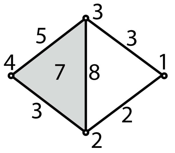
It is easy to show (see [6], Lemma 2.5) that, for a discrete Morse function, $c^{+}(\sigma)$ and $c^{-}(\sigma)$ cannot be simultaneously equal to 1. A $k$-simplex $\sigma$ in $\Sigma$ is called critical simplex of index $k$ (or, $k$-saddle) if $c^{+}(\sigma)=c^{-}(\sigma)=0$. A critical simplex of index $0$ is called a minimum, while a critical simplex of index $d=dim(\Sigma)$ a maximum. Figure 4(a) shows a discrete Morse function $f$ defined on a simplicial complex. Each simplex is labeled with the corresponding value of function $f$. Vertex 1 is critical (minimum), since $f$ has a higher value on all edges incident to it. Edge 5 is critical (saddle), since $f$ has a higher value on the incident triangle 7, and lower values on its vertices.

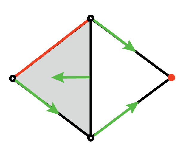
A discrete vector field $V$ on $\Sigma$ is a collection of pairs of simplices $(\sigma,\tau)\in\Sigma\times\Sigma$ such that $\sigma\in bd(\tau)$ and each simplex of $\Sigma$ is in at most one pair of $V$. A discrete Morse function $f:\Sigma\rightarrow{\mathbb{R}}$ induces a discrete vector field $V=\{(\sigma,\tau)\in\Sigma\times\Sigma\,|\,\sigma\in bd(\tau)\text{ and }f(\sigma)\geq f(\tau)\}$, called a Forman gradient (or, equivalently, gradient vector field) of $f$ on $\Sigma$. A pair $(\sigma,\tau)\in V$ can be depicted as an arrow from $\sigma$ to $\tau$. Given a discrete vector field $V$, a $V$-path (or, equivalently, a gradient path) is a sequence $[(\sigma_{1},\tau_{1}),(\sigma_{2},\tau_{2}),\dots,(\sigma_{r},\tau_{r})]$ of pairs of $k$-simplices $\sigma_{i}$ and $(k+1)$-simplices $\tau_{i}$, such that $(\sigma_{i},\tau_{i})\in V$, $\sigma_{i+1}$ is a face of $\tau_{i}$, and $\sigma_{i}\neq\sigma_{i+1}$. A $V$-path is a closed path if $\sigma_{1}$ is a face of $\tau_{r}$ different from $\sigma_{r}$. It has been proven that a discrete vector field $V$ is the Forman gradient of a discrete Morse function if and only if $V$ is free of closed paths [6].

Given a Forman gradient $V$ on a simplicial complex $\Sigma$, the discrete Morse complex associated with $\Sigma$ is a chain complex $\mathcal{M}_{*}:=(\mathcal{M}_{k},\tilde{\partial}_{k})_{k\in{\mathbb{Z}}}$, where:

• •

  groups $\mathcal{M}_{k}$ are generated by the critical $k$-simplices;

• •

  the boundary maps $\tilde{\partial}_{k}$ are obtained by following the gradient paths of $V$ (see Subsection 8.2 for a detailed description).

A discrete Morse complex $\mathcal{M}_{*}$, associated with a simplicial complex $\Sigma$, provides a homologically equivalent representation of $\Sigma$ (see [6], Theorem. 8.2). If we consider a simplicial complex $\Sigma$, and we compute a Forman gradient $V$ on it (see Figure 5(a)), we obtain a discrete Morse complex $\mathcal{M}_{*}$ having its cells in one-to-one correspondence with the critical simplices of $V$. $\mathcal{M}_{*}$ can be described as a graph having nodes in correspondence of the critical simplices of $V$, and having the arcs in one-to-one correspondence with the gradient paths connecting such nodes (see Figure 5(b)).

Since $\Sigma$ and $\mathcal{M}_{*}$ are homologically equivalent, computing the homology on $\mathcal{M}_{*}$ is preferable due to the fact that the cells in $\mathcal{M}_{*}$ are generally fewer than the simplices in $\Sigma$. As shown in [32], the homological equivalence between a simplicial complex $\Sigma$ and a discrete Morse complex $\mathcal{M}_{*}$ associated with $\Sigma$ can be generalized to persistent homology by requiring that the Forman gradient $V$ is filtered with respect to the filtration $F$ considered. Formally, given a filtration $F=\{\Sigma^{m}\,|\,0\leq m\leq M\}$ of a simplicial complex $\Sigma$, a Forman gradient $V$ of $\Sigma$ is filtered with respect to $F$ if, for each pair $(\sigma,\tau)\in V$, there exists $m\in\{1,\dots,M\}$ such that $\sigma$, $\tau\in\Sigma^{m}$ and $\sigma$, $\tau\notin\Sigma^{m-1}$.

Several topological data structures for encoding a simplicial complex have been proposed in the literature, mainly for simplicial complexes in low dimensions, and focusing on triangle and tetrahedral meshes (see [33] for a survey). We consider here data structures specific for simplicial complexes in arbitrary dimensions.

The most general dimension-independent data structure for cell and simplicial complexes is the Incidence Graph. An Incidence Graph ($IG$) [34] is a topological incidence-based representation of a simplicial complex which encodes all the simplices as nodes of a graph and their immediate boundary and coboundary relations as its arcs. The Simplified Incidence Graph ($SIG$) [35] and the Incidence Simplicial ($IS$) data structures [36] are simplified representations of the $IG$. A comparison among $IG$, $SIG$ and $IS$ is presented in [37], while an implementation of all these data structures is included in the Mangrove Topological Data Structure library available in the public domain [38].

In the case of triangle and tetrahedral meshes, adjacency-based data structures are the most widely used thanks to their compactness and efficiency. The Generalized Indexed data structure with Adjacencies ($IA^{*}$) [17] generalizes such representations and is capable of encoding non-manifold simplicial complexes of any dimension. Recently, a topological data structure has been proposed for simplicial complexes embedded in the Euclidean space in [39], where topological relations can be efficiently extracted in parallel on different portions of the domain.

In recent years, new data structures have been developed well suited to perform specific tasks. The Simplex Tree (ST) [40] has been defined to efficiently extract boundary relations for computing persistent homology. The Simplex Tree encodes all simplices in the complex and tends to be more verbose than the $IA^{*}$ data structure, as shown in [39]. An implementation of the $ST$ is available in the Gudhi public domain library [41]. The Maximal Simplex Tree (MST) and the Simplex Array List (SAL) [42] are optimized versions of the $ST$. To the extent of our knowledge, there are no implementations of these data structures. The skeleton blocker data structure [43] has been created specifically to perform edge contraction on a simplicial complex, but it can be efficiently initialized only when working with flag complexes. An implementation of the latter is provided in the Gudhi library [41].

The process of building a discrete Morse complex from a simplicial complex typically consists of two steps: (i) computing the Forman gradient and identifying the critical simplices, and (ii) extracting the boundary maps. We can classify algorithms for computing a Forman gradient as: unconstrained [44, 45, 46, 47, 11, 48] and constrained algorithms [49, 50, 51, 10, 52, 53, 54, 55]. Unconstrained algorithms compute a Forman gradient on a cell/simplicial complex when no scalar value is provided. The aim is to create a homologically equivalent representation of the input complex having as few critical cells as possible. Constrained algorithms start from a cell/simplicial complex endowed with a scalar function $F_{0}$ defined on its vertices, and aim at constructing a Forman gradient that best fits $F_{0}$ [50, 51, 10, 52]. The discrete Morse complex is used in the analysis and visualization of scalar fields as a compact representation of the field behavior. The aim is to obtain a decomposition of the dataset in regions of influence for each critical simplex. Ascending and descending traversal techniques [55, 56, 57] for the $V$-paths of the Forman gradient have been developed for reconstructing the ascending and descending Morse cells, respectively. We refer to [9] for an in-depth description of these methods. When computing persistent homology on a simplicial complex $\Sigma$ [58, 59, 60], the aim is to obtain a complex which is a compact version of $\Sigma$ and has the same persistent homology [10, 32, 61]. To this aim, the gradient V-paths need to be visited by starting from the critical simplices and by traversing the paths in a descending manner. A detailed description of this process is provided in Subsection 8.2.

We analyze here three data structures for encoding a simplicial complex, namely the Incidence Graph ($IG$) [34], the Simplex Tree ($ST$) [40, 62], and the Generalized Indexed data structure with Adjacencies ($IA^{*}$ data structure) [17]. The $IG$ is the most widely-used data structure for simplicial complexes, the $ST$ has been used in topological data analysis applications, being implemented in the Gudhi library, the $IA^{*}$ data structure is a compact representation for simplicial complexes encoding only vertices and top simplices. Implementations in the public domain exist for all of them, and on such implementations we base our experimental comparisons.

The Incidence Graph ($IG$) for complex $\Sigma$ describes its Hasse diagram [63], i.e., the graphical representation of the partially ordered set generated by all the simplices of $\Sigma$ and their incidence relations. The $IG$ can be viewed as a directed graph $G_{IG}=(N_{IG},B_{IG}\cup C_{IG})$ in which:

• •

  the nodes in $N_{IG}$ are in one-to-one correspondence with the simplices of $\Sigma$; with abuse of notation, we will indicate with $\sigma$ both a node, and its corresponding simplex;

• •

  a directed arc in $B_{IG}$ (boundary arc) connects two nodes ($\tau,\sigma$) in $N_{IG}$ with $dim(\tau)=dim(\sigma)+1$ if $\sigma$ is a face of $\tau$;

• •

  a directed arc (coboundary arc) in $C_{IG}$ connects two nodes ($\sigma,\tau$) in $N_{IG}$ with $dim(\tau)=dim(\sigma)+1$ if $\tau$ is a coface of $\sigma$.

In Figure 6(b), the $IG$ representing the simplicial complex $\Sigma$ depicted in Figure 6(a) is shown. Nodes are colored according to the dimension of the simplex they represent. Note that, for simplicity, we have shown only one undirected arc for each pair of mutual incident nodes, since if a directed arc exists from $\tau$ to $\sigma$ in $B_{IG}$, arc $(\sigma,\tau)$ must exist in $C_{IG}$ By storing the incidence relations between simplices of consecutive dimension, the $IG$ is efficient in the retrieval of topological relations, but the large amount of information encoded makes it unsuitable for complexes of large size and of high dimensions [37].

The Simplex Tree ($ST$) [40] encodes also all the simplices of a simplicial complex $\Sigma$ as the $IG$, but only a subset of the incidence relations encoded in the $IG$. The $ST$ is based on a total order selected on the vertices of $\Sigma$. Let $I(v)$ be the position in the total order of a vertex $v\in\Sigma$. Given a $k$-simplex $\sigma=\{v_{0},...,v_{k}\}$ in $\Sigma$, $max_{v}(\sigma)=max(I(v_{i}))$ is the latest vertex of $\sigma$ in the total order. The $ST$ can be viewed as a graph $G_{ST}=(N_{ST},A_{ST})$ in which:

• •

  the nodes in $N_{ST}$ are in one-to-one correspondence with the simplices of $\Sigma$, and a node $\sigma\in N_{ST}$ is labeled with $I(max_{v}(\sigma))$;

• •

  a directed arc $(\sigma,\tau)\in A_{ST}$ connects two nodes in $N_{ST}$, if $\sigma$ is in the immediate boundary of $\tau$, and $I(max_{v}(\tau))>I(max_{v}(\sigma))$.

Nodes corresponding to the vertices of $\Sigma$ are connected to the root of the Simplex Tree. If we select a path from the root to a node $\sigma=\{v_{0},...,v_{k}\}$, we have that: (i) labels $\{l_{0},...,l_{k}\}$ are encountered sorted by increasing order along the path and each label appears exactly once; (ii) each label corresponds to a vertex of $\sigma$, more precisely $l_{i}=I(v_{i})$, for each $i=0,...,k$.

In Figure 6(c), we show the Simplex Tree representation of the simplicial complex depicted in Figure 6(a). The order of the vertices is indicated by the numbers depicted in blue, while the remaining numbers indicate the labels of the nodes corresponding to the $k$-simplices, with $k>0$. For the sake of clarity, we are not showing the connections between the vertices and the root. Note that the Simplex Tree is order dependent, in the sense that we can have different $ST$s for the same complex. For example, Figure 6(d) shows the $ST$ obtained for $\Sigma$ by using a different order for its vertices.

From the two graph representations, we see that $N_{IG}=N_{ST}$ and that $A_{ST}\subset A_{CB}$, since it contains all those arcs $(\sigma,\tau)\in A_{CB}$ for which $I(max_{v}(\tau))>I(max_{v}(\sigma))$. The Simplex Tree has been designed with the task of efficiently performing only boundary queries. In order to be able to perform also coboundary queries, an extended version of the Simplex Tree has been proposed in [40]. This extended version contains a circular list linking all the nodes having the same label and the same dimension and an arc from a node to its parent. This version is not implemented in the Simplex Tree in the public domain library Gudhi [41]. In [42], two compressed optimization of the latter have been presented, namely the Maximal Simplex Tree and the Simplex Array List, sharing the same functionalities but reducing the number of nodes encoded. To the best of our knowledge, no implementations are provided for these latter.

As mentioned before, more compact representations for a simplicial complex can be obtained by encoding only the vertices and top simplices. To be able to extract boundary, coboundary and adjacency relations efficiently, the simplest representation would encode: (i) for each top $k$-simplex $\sigma$, its boundary defined by the references to its $k+1$ vertices, and its adjacencies defined by references to the simplices adjacent to $\sigma$ along a $(k-1)$-face; (ii) for each vertex $v$, its star, defined by the the list of all top simplices incident in $v$. It can be noticed that storing the entire star of a vertex $v$ is not necessary, since the star can be efficiently reconstructed by navigating the top simplices incident in $v$ through the encoded adjacencies. This constitutes the basis for the Generalized Indexed data structure with Adjacencies ($IA^{*}$) [17].

We can describe the $IA^{*}$ data structure as a graph $G_{IA}=(N_{IA},A_{IA})$ in which $N_{IA}=N_{0}\cup N_{top}$, with set $N_{0}$ corresponding to the vertices of $\Sigma$, and set $N_{top}$ corresponding to the top simplices of $\Sigma$. The set of arcs in $A_{IA}$ is the disjoint union of three subsets $A_{(t,0)}$,$A_{(t,t)}$, $A_{(0,t)}$ defined as follows:

• •

  $A_{(t,0)}$ (boundary arcs): a directed arc $(\sigma,v)$, where $\sigma$ is in $N_{top}$ and $v$ in $N_{0}$, belongs to $A_{(t,0)}$ if $v$ is a vertex of $\sigma$;

• •

  $A_{(t,t)}$ (adjacency arcs): an undirected arc $(\sigma,\tau)$, where $\sigma$ and $\tau$ are $k$-simplices in $N_{top}$, belongs to $A_{(t,t)}$ if $\sigma$ and $\tau$ share a $(k-1)$-face;

• •

  $A_{(0,t)}$ (coboundary arcs): a subset of the arcs $(v,\sigma)$, where $v$ in $N_{0}$ and $\sigma$ is in $N_{top}$, such that $v$ is on the coboundary of $\sigma$, as defined below.

Given a vertex $v$, we consider the subgraph $G_{IA}(v)=(N_{IA}(v),A_{IA}(v))$ of $G_{IA}$ where:

• •

  $N_{IA}(v)$ consists of all nodes $\sigma\in N_{top}$ such that $v$ is a vertex of $\sigma$;

• •

  $A_{IA}(v)$ consists of all arcs in $A_{(t,t)}$ connecting pair of nodes in $N_{IA}(v)$.

Thus, an oriented arc $(v,\sigma)$ is encoded in $A_{(0,t)}$ for each connected component in $G_{IA}(v)$, where $\sigma$ is any top simplex in $N_{IA}(v)$ belonging to such component.

In Figure 7, we show the nodes and the arcs encoded in the $IA^{*}$ data structure (see Figure 7(b)) for the simplicial complex in Figure 7(a). Blue nodes denote vertices, while green and red nodes denote top edge and triangles, respectively. Undirected arcs represent adjacency relations among top simplices, i.e., arcs $(\tau_{1},\tau_{2})$ and $(\sigma_{1},\sigma_{2})$. Boundary arcs are denoted by arrows, while coboundary arcs by dotted arrows.

The space required by the $IA^{*}$ data structure depends on the structure on the complex, i.e., the number of arcs in $A_{(t,t)}$ and in $A_{(0,t)}$ depends on the connectivity of the top simplices. If we restrict our consideration to an important subclass of simplicial complexes, that of simplicial pseudomanifolds, we can get some insights for comparing the space required by the $IA^{*}$ data structure to that of the $IG$. Recall that a simplicial $d$-pseudomanifold is a $(d-1)$-connected simplicial $d$-complex such that any $(d-1)$-simplex is on the boundary of either one or two $d$-simplices.

If $\Sigma$ is a $d$-pseudomanifold, we have that the number of arcs in $A_{(t,0)}$ originating from a top $k$-simplex $\sigma$ is equal to $k+1$. The number of arcs in $A_{(t,t)}$ originating from a top $k$-simplex $\sigma$ is also equal to $k+1$. Thus, $|A_{(t,t)}|$ is equal to $|A_{(t,0)}|$ and, thus, the total cost of storing the boundary and the adjacency arcs in the $IA^{*}$ data structure is equal to $2|A_{(t,0)}|$. We can observe that $c=2|A_{(t,0)}|$ is exactly the cost of storing in the $IG$ all the boundary arcs connecting a $d$-simplex to a $(d-1)$-simplex plus all the dual coboundary arcs connecting a $(d-1)$-simplex to a $d$-simplex. In the $IA^{*}$ data structure, besides $c$, we have the cost $c_{st}$ of storing some top simplices in the star of the vertices. For each vertex $v$, $c_{st}$ is equal to the number of connected components of $G_{IA}(v)$. In the worst case this might be equal to the number of $d$-simplices having $v$ on their boundary. However, in the $IG$ we need to take into account the cost of encoding the other boundary and coboundary arcs which connect $k$- and $(k-1)$-simplices (with $k<d$), which will be clearly much higher than $c_{st}$.

This subsection provides an experimental comparison among the $IG$, the $ST$ and the $IA^{*}$ data structure. In our experiments, we have used three kinds of data sets. The first data sets are volume data that have been tetrahedralized. Each vertex of the dataset has an associated scalar value. The DTI-scan is a Diffusion Tensor MRI Scan of a human brain, the VisMale dataset is a CT-scan of a man’s head and the Ackley dataset is a synthetic function discretizing Ackley’s function [64]. The datasets in the second group are networks obtained from real data on which cliques have been computed. Two of these datasets (Amazon1, Amazon2) are graphs representing the “Customers Who Bought This Item Also Bought" feature of the Amazon website. If a product $i$ is frequently co-purchased with product $j$, the graph contains a directed edge from $i$ to $j$ (notice, we are considering the graph undirected). The third graph represents a road network in California where intersections and endpoints are described by nodes and the roads connecting these intersections or road endpoints are described by undirected edges (roadnet). The datasets in the third group are point clouds extracted from a 2-sphere on which a Vietoris-Rips complex has been computed (datasets S1.0, S1.2, S1.3).

In our comparisons, we use the Simplex Tree (ST) implementation in the Gudhi library [41], the Incidence Graph (IG) implemented in Perseus [18], which is a public domain tool for computing the discrete Morse complex, and the $IA^{*}$ data structure implemented in [65]. Table 1 summarizes the characteristics of the datasets we used and their storage costs using the three data structures. For each dataset, we provide the dimension of the resulting simplicial complex (column $d$), the number of its vertices (column $|\Sigma_{0}|$) and of its top simplices (column $|\Sigma_{top}|$), the size of the complex (column $|\Sigma|$), and the storage cost required by the three data structures, expressed in gigabytes.

We can observe that the storage cost of the $IG$ and of the $ST$ increases based on the total number of simplices. The $IG$ implemented in the Perseus library often runs out of memory, while the $ST$ has much higher limits. The storage cost of the $IA^{*}$ data structure depends on the number of top simplices. This means that simplicial complexes in low dimensions (like Roadnet or the volumetric datasets) may require comparatively more memory than, for example, Sphere-1.3 (being a 23-simplicial complex composed by less than 400 top simplices). It is clear that the $IA^{*}$ data structure is always more compact than the $ST$. The ratio between the storage costs of the two data structures roughly depends on the ratio between the number of top simplices and the size of the complex. The worst-case scenario occurs for (Roadnet dataset) where the $IA^{*}$ data structure requires 20% less memory than the $ST$, while in the case of Sphere-1.3 the storage cost for the $IA^{*}$ data structure is negligible with respect to the 11 gigabytes required by the $ST$.

In this subsection, we describe how to encode a discrete gradient field, like the Forman gradient $V$, on the data structures encoding a simplicial complex $\Sigma$.

If we consider the Incidence Graph $G$ representing $\Sigma$, we see that the arcs of $G$ describe all the possible pairings that can be defined on $\Sigma$ by considering two simplices of consecutive dimension. A Forman gradient can be encoded on the $IG$ by adding one bit flag to each arc $a$ in $C_{IG}$ indicating whether the nodes incident in $a$ are also a valid pair in $V$. Because of this reason, the $IG$ has been selected in the Perseus tool [18]. This encoding cannot be extended to the Simplex Tree since this latter encodes only a subset of the coboundary arcs of the $IG$.

We describe here a new representation which allows for a compact encoding of a Forman gradient on the $IA^{*}$ data structure and, in general, for any data structure which encodes vertices plus top simplices. In this case, the encoding for the gradient pairs needs to be attached to the top simplices only. The representation that we have defined encodes, for each top $k$-simplex $\tau$, a bit-vector of length $\sum_{i=1}^{k}{\binom{k+1}{i+1}(i+1)}$ representing all the possible pairings on its boundary. The first $k+1$ bits encode the pairing between $\tau$ and one of its $(k-1)$-faces. Then, recursively, for each $i$-face of $\tau$, $i+1$ bits are stored until, for each 1-face, 2 bits are encoded storing the pairings with one of its vertices. For example, considering a 2-simplex (triangle), 3 bits are reserved for encoding the pairings with the boundary edges. Then, for each of them, 2 bits are reserved for encoding the pairings with the boundary vertices (see Figure 8).

If two paired simplices $\rho$ and $\sigma$ are both on the boundary of $\tau$, the resulting pair will be encoded in the bit-vector of $\tau$. Let $j$ and $l$ (with $j+1=l$) be the dimensions of $\rho$ and $\sigma$, respectively, we check the bit associated with the corresponding pair computing:

• •

  the position $\sum_{i=l+1}^{k}{\binom{k+1}{i+1}(i+1)}$ of the first bit reserved for $l$-simplices in $\tau$;

• •

  the position of $\sigma$ on the boundary of $\tau$ obtained enumerating the faces of $\tau$;

• •

  the position of the vertex in $\sigma$ that is not in $\rho$.

For example, in Figure 8, we consider the pairing between the 0-simplex $v_{0}$ and the 1-simplex $v_{0}v_{2}$. The bits reserved for the $1$-simplices start at position 3. The position of $v_{0}v_{2}$ on the boundary of the triangle is 1, so we discard the first two bits. Vertex $v_{2}$ is missing in $v_{0}$ and its position is 1. Then, the bit representing their pairing relation is at position $3+(2\cdot 1)+1$.

We have implemented a prototype of the gradient encoding based on the dynamic_bitset provided by the Boost C++ library. With such encoding, we have been able to represent the gradient frame representation up to 40-dimensional simplicial complexes. Using more involved libraries and architectures could overcome the current limitations, but it might greatly affect computation times.

The theoretical equivalences proven in Section 6 and Section 7 tell us that there is no preferable homology-preserving operator for computing a Forman gradient. Here, we introduce a new dimension-independent algorithm, that can also runs in parallel, which uses a representation of the simplicial complex as an $IA^{*}$ data structure and the encoding of the Forman gradient discussed in Subsection 4.

The basic underlying approach is the coreduction-based algorithm, introduced in [11] and implemented there only for regular grids. We summarize it for simplicial complexes. When considering simplicial complexes, the coreduction-based algorithm computes a Forman gradient by using coreduction pairs starting from the simplices of lowest dimension. The set of $k$-simplices of complex $\Sigma$ is considered by increasing values of $k$, starting from $k=0$. As long as a coreduction pair exists between a $k$-simplex $\sigma$ and a $(k+1)$-simplex $\tau$, pair $(\sigma,\tau)$ is added to the Forman gradient $V$. When no $k$-simplex can be paired, one simplex is randomly chosen and declared critical. When all $k$-simplices have been paired or denoted as critical, the working dimension $k$ is increased by one. Since no coreduction pair is feasible on a simplicial complex, at the first step, an arbitrary vertex $v$ is denoted as critical in $V$ to trigger coreductions. In [32], the coreduction-based approach is used for persistent homology computation, and thus by considering a filtration of the original complex. If each simplex is paired only with another simplex belonging to the same filtration value, the resulting discrete Morse complex will have the same persistent homology of the original complex.

The dimension-independent coreduction-based algorithm proposed here, unlike previous ones, uses a local approach that allows us to work on the stars of the vertices independently, which makes it particularly suitable for a parallel implementation. We define an indexing on the vertices of the input simplicial complex $\Sigma$, and we extend the indexing to all the simplices in such a way that each simplex in $\Sigma$ has an index equal to the maximum of the indexes of its vertices. With such indexing, the coreduction pairs can be computed locally to the lower star of each vertex. Given a vertex $v$, a simplex $\sigma$ belongs to the lower star of $v$ (denoted as $St^{-}(v)$) if: (i) $\sigma$ is a coface of $v$, and (ii) $v$ has lowest index value among the vertices of $\sigma$. Algorithm 1 illustrates the process for computing a Forman gradient on a simplicial complex $\Sigma$ having an indexing $F_{0}$ defined on its vertices.

The algorithm iterates on the vertices of $\Sigma$, extracting first the top simplices in the lower star of $v$, denoted as $LT_{v}$, which are encoded in a list. For each vertex $v$, the algorithm iterates on the dimension of the simplices in the lower star of $v$. The algorithm works, for each dimension, with two sets of simplices: the set of $k$-simplices that can be declared critical, denoted as $CR_{v}$ (row 12), and the set of $(k+1)$-simplices to pair (row 14), denoted as $ST_{v}$. $CR_{v}$ and $ST_{v}$ have a maximum size equal to the maximum, by varying $k$, of the number of $k$-simplices in the lower star of a vertex in $\Sigma$, and they are encoded as balanced binary search trees. A candidate simplex is extracted from set $ST_{v}$ (row 16) and paired with its unique unpaired face (row 18). Recall that a simplex $\tau$ can be paired with another simplex $\sigma$ by coreduction if $\sigma$ is the only unpaired face of $\tau$. If there are no coreductions available (row 21), a new critical simplex is taken from $CR_{v}$. Every time a simplex is paired or set as critical, it is also removed from $ST_{v}$ or $CR_{v}$, respectively. When set $CR_{v}$ is empty, the working dimension is increased. The algorithm terminates when all the simplices in the lower star of each vertex $v$ have been paired, or set as critical.

The procedures and the functions, on which Algorithm 1 is based, are:

• •

  Function $LowerTop(v,\Sigma,F_{0})$: computes all the top simplices of $\Sigma$ belonging to the lower star of $v$ and encodes such simplices in list $LT_{v}$. This is performed by navigating the star of vertex $v$ through the adjacency arcs in the $IA^{*}$ data structure. Thus, it works in time $O(t_{v})$, where $t_{v}$ denotes the number of top simplices in the star of $v$.

• •

  Function $LowerStar(v,\Sigma,F_{0},LT_{v},k)$: extracts all the $k$-simplices belonging to the lower star of $v$ from $LT_{v}$ and encodes such simplices in $ST_{v}$. This operation is performed by cycling on the elements of $LT_{v}$ and collecting the $k$-faces of each top simplex that are also incident in $v$. The extraction of the $k$-simplices of a top simplex of dimension $i$ is performed in $O({{i+1}\choose{k+1}})$. If we denote as $t_{v,i}$ the number of top simplices of dimension $i$ incident in $v$, the total number $N_{k}$ of simplices extracted is $N_{k}=\sum_{i=1}^{d}t_{v,i}{{i+1}\choose{k+1}})$ in the worst case, since some simplices are contained within the boundary of more than one top simplex. Since each of such simplices is inserted in $ST_{v}$, $LowerStar(v,\Sigma,F_{0},LT_{v},k)$ may require $O(N_{k}\log N_{k})$ time in the worst case.

• •

  Procedure $addPair(\sigma,\tau,V)$: adds a new pair to $V$. Since the gradient pairs are encoded on the top simplices only, we have to find the top simplices incident in both $\sigma$ and $\tau$. This is done by examining all the top simplices in the star of a vertex of $\sigma$ and detecting all those having $\tau$ on their boundary. For each of these latter, we update the corresponding bit-vector. The operation requires $O(t_{w})$, where $t_{w}$ denotes the number of top simplices incident in a vertex $w$ of $\sigma$.

• •

  Function $getNextPair(v,\Sigma,ST_{v},CR_{v})$: iterates on the set of unpaired simplices $ST_{v}$ selecting the first simplex available for a coreduction. For each simplex $\tau$ in $ST_{v}$, the simplices on the boundary of $\tau$ containing $v$ are extracted, and then, for each of such boundary simplices $\sigma$, the membership of $\sigma$ to $CR_{v}$ is checked. In the worst case, we will need to check the membership of all the elements in $CR_{v}$. This leads to a worst-case complexity of $O(k|ST_{v}||CR_{v}|\log|CR_{v}|)$.

• •

  Function $getFirstCritical(CR_{v})$: returns the first simplex in the set of candidate critical simplices $CR_{v}$. Since $CR_{v}$ is implemented as a balanced binary search tree, the worst-case time complexity is $O(\log|CR_{v}|)$.

• •

  Procedure $Remove(\sigma,CR_{v})$: eliminates a simplex from $CR_{v}$ (or $ST_{v}$). Since both $CR_{v}$ and $ST_{v}$ are implemented as a balanced binary search tree, the worst-case time complexity is $O(\log|CR_{v}|)$.

References

- [1] V. De Silva, R. Ghrist, Homological sensor networks, Notices of the American Mathematical Society 54.
- [2] R. Fellegara, U. Fugacci, F. Iuricich, L. De Floriani, Analysis of geolocalized social networks based on simplicial complexes, in: 9th ACM SIGSPATIAL International Workshop on Location-Based Social Networks (LSBN), ACM, 2016.
- [3] S. Martin, A. Thompson, E. A. Coutsias, J.-P. Watson, Topology of cyclo-octane energy landscape, Journal of Chemical Physics 132 (23) (2010) 234115.
- [4] R. van de Weygaert, G. Vegter, H. Edelsbrunner, B. J.-T. Jones, P. Pranav, C. Park, W. A. Hellwing, B. Eldering, N. Kruithof, E. Bos, et al., Alpha, Betti and the Megaparsec universe: on the topology of the cosmic web, in: Transactions on Computational Science XIV, Springer, 2011, pp. 60–101.
- [5] M. K. Chung, P. Bubenik, P. T. Kim, Persistence diagrams of cortical surface data, in: Information Processing in Medical Imaging, Springer, 2009, pp. 386–397.
- [6] R. Forman, Morse theory for cell complexes, Advances in Mathematics 134 (1) (1998) 90–145.
- [7] P. Frosini, M. Pittore, New methods for reducing size graphs, International Journal of Computer Mathematics 70 (3) (1999) 505–517.
- [8] A. J. Zomorodian, The tidy set: a minimal simplicial set for computing homology of clique complexes, in: Proceedings of the 2010 Annual Symposium on Computational Geometry, ACM, 2010, pp. 257–266.
- [9] L. De Floriani, U. Fugacci, F. Iuricich, P. Magillo, Morse complexes for shape segmentation and homological analysis: discrete models and algorithms, Computer Graphics Forum 34 (2) (2015) 761–785.
- [10] V. Robins, P. J. Wood, A. P. Sheppard, Theory and algorithms for constructing discrete Morse complexes from grayscale digital images, IEEE Transactions on Pattern Analysis and Machine Intelligence 33 (8) (2011) 1646–1658.
- [11] S. Harker, K. Mischaikow, M. Mrozek, V. Nanda, Discrete Morse theoretic algorithms for computing homology of complexes and maps, Foundations of Computational Mathematics 14 (1) (2014) 151–184.
- [12] S. Harker, K. Mischaikow, M. Mrozek, V. Nanda, H. Wagner, M. Juda, P. Dłotko, The efficiency of a homology algorithm based on discrete Morse theory and coreductions, in: Proceedings 3rd International Workshop on Computational Topology in Image Context (CTIC 2010). Image A, Vol. 1, 2010, pp. 41–47.
- [13] C. Correa, P. Lindstrom, P.-T. Bremer, Topological spines: a structure-preserving visual representation of scalar fields, IEEE Transactions on Visualization and Computer Graphics 17 (12) (2011) 1842–1851.
- [14] M. Allili, T. Kaczynski, C. Landi, Reducing complexes in multidimensional persistent homology theory, Journal of Symbolic Computation 78 (2017) 61 – 75.
- [15] M. Allili, T. Kaczynski, C. Landi, F. Masoni, Algorithmic construction of acyclic partial matchings for multidimensional persistence, Springer, 2017, pp. 375–387.
- [16] U. Fugacci, F. Iuricich, L. De Floriani, Efficient computation of simplicial homology through acyclic matching, in: Symbolic and Numeric Algorithms for Scientific Computing (SYNASC), 2014 16th International Symposium on, 2014, pp. 587–593.
- [17] D. Canino, L. De Floriani, K. Weiss, : an adjacency-based representation for non-manifold simplicial shapes in arbitrary dimensions, Computers & Graphics 35 (3) (2011) 747–753.
- [18]
V. Nanda, The
Perseus software project for rapid computation of persistent
homology.
URL http://www.math.rutgers.edu/˜vidit/perseus/index.html - [19] A. T. Lundell, S. Weingram, The topology of CW complexes, Van Nostrand Reinhold Company, 1969.
- [20] H. Edelsbrunner, D. G. Kirkpatrick, R. Seidel, On the shape of a set of points in the plane, IEEE Transactions on Information Theory 29 (4) (1983) 551–559.
- [21] E. W. Chambers, V. De Silva, J. Erickson, R. Ghrist, Vietoris-Rips complexes of planar point sets, Discrete & Computational Geometry 44 (1) (2010) 75–90.
- [22] A. Hatcher, Algebraic topology, Cambridge University Press, 2002.
- [23] A. J. Zomorodian, Fast construction of the Vietoris-Rips complex, Computer and Graphics (2010) 263–271.
- [24] V. De Silva, G. Carlsson, Topological estimation using witness complexes, in: Proceedings of the First Eurographics Conference on Point-Based Graphics, 2004, pp. 157–166.
- [25] V. De Silva, A weak definition of Delaunay triangulation, arXiv preprint cs/0310031.
- [26] L. J. Guibas, S. Y. Oudot, Reconstruction using witness complexes, Discrete & Computational geometry 40 (3) (2008) 325–356.
- [27] T. K. Dey, F. Fan, Y. Wang, Graph induced complex on point data, in: Proceedings of the Twenty-ninth Annual Symposium on Computational Geometry, SoCG ’13, 2013, pp. 107–116.
- [28] H. Edelsbrunner, J. Harer, Persistent homology - a survey, Contemporary Mathematics 453 (2008) 257–282.
- [29] A. J. Zomorodian, Topology for computing, Cambridge University Press, 2005.
- [30] R. Ghrist, Barcodes: the persistent topology of data, Bulletin of the American Mathematical Society 45 (1) (2008) 61–75.
- [31] R. Forman, A user’s guide to discrete Morse theory, Séminaire Lotharingien de Combinatoire 48 (2002) 35.
- [32] K. Mischaikow, V. Nanda, Morse theory for filtrations and efficient computation of persistent homology, Discrete & Computational Geometry 50 (2) (2013) 330–353.
- [33] L. De Floriani, A. Hui, Data structures for simplicial complexes: an analysis and a comparison, in: M. Desbrun, H. Pottmann (Eds.), Proc. 3rd Eurographics Symposium on Geometry Processing, 2005, pp. 119–128.
- [34] H. Edelsbrunner, Algorithms in combinatorial geometry, Springer, 1987.
- [35] L. De Floriani, D. Greenfieldboyce, A. Hui, A data structure for non-manifold simplicial d-complexes, in: Proceedings of the 2004 Eurographics/ACM SIGGRAPH Symposium on Geometry processing, ACM, 2004, pp. 83–92.
- [36] L. De Floriani, A. Hui, D. Panozzo, D. Canino, A dimension-independent data structure for simplicial complexes, Proceedings of the 19th International Meshing Roundtable (2010) 403–420.
- [37] D. Canino, L. De Floriani, Representing simplicial complexes with Mangrove, Proceedings of the 22nd Iinternational Meshing Roundtable (2013) 465–483.
- [38]
D. Canino, The Mangrove TDS
Library: a C++ tool for fast prototyping of topological data structures
(2012).
URL http://mangrovetds.sourceforge.net - [39] R. Fellegara, K. Weiss, L. De Floriani, The Stellar tree: a compact representation for simplicial complexes and beyond, arXiv preprint arXiv:1707.02211.
- [40] J.-D. Boissonnat, C. Maria, The Simplex Tree: an efficient data structure for general simplicial complexes, Algorithmica 70 (3) (2014) 406–427.
- [41] C. Maria, J.-D. Boissonnat, M. Glisse, M. Yvinec, The GUDHI library: simplicial complexes and persistent homology, in: H. Hong, C. Yap (Eds.), Mathematical Software â ICMS 2014, Springer, 2014, pp. 167–174.
- [42] J.-D. Boissonnat, K. C. S., S. Tavenas, Building efficient and compact data structures for simplicial complexes, in: L. Arge, J. Pach (Eds.), 31st International Symposium on Computational Geometry, 2015, pp. 642–656.
- [43] D. Attali, A. Lieutier, D. Salinas, Efficient data structure for representing and simplifying simplicial complexes in high dimensions, in: Proceedings of the 27th ACM Symposium on Computational Geometry, 2011, pp. 501–509.
- [44] T. Lewiner, H. Lopes, G. Tavares, Optimal discrete Morse functions for 2-manifolds, Computational Geometry 26 (3) (2003) 221 – 233.
- [45] M. Mrozek, B. Batko, Coreduction homology algorithm, Discrete & Computational Geometry 41 (1) (2009) 96–118.
- [46] M. Mrozek, T. Wanner, Coreduction homology algorithm for inclusions and persistent homology, Comput. Math. Appl. 60 (10) (2010) 2812–2833.
- [47] P. Dłotko, T. Kaczynski, M. Mrozek, T. Wanner, Coreduction homology algorithm for regular CW-complexes, Discrete & Computational Geometry 46 (2) (2011) 361–388.
- [48] B. Benedetti, F. H. Lutz, Random discrete Morse theory and a new library of triangulations, Experimental Mathematics 23 (1) (2014) 66–94.
- [49] F. Cazals, F. Chazal, T. Lewiner, Molecular shape analysis based upon the Morse-Smale complex and the Connolly function, in: Proc. 9th Annual Symposium on Computational Geometry, 2003, pp. 351–360.
- [50] H. King, K. Knudson, N. Mramor, Generating discrete Morse functions from point data, Experimental Mathematics 14 (4) (2005) 435–444.
- [51] A. Gyulassy, P.-T. Bremer, B. Hamann, V. Pascucci, Practical considerations in Morse-Smale complex computation, in: V. Pascucci, X. Tricoche, H. Hagen, J. Tierny (Eds.), Topological Methods in Data Analysis and Visualization: Theory, Algorithms, and Applications, Mathematics and Visualization, Springer, 2011, pp. 67–78.
- [52] A. Gyulassy, P.-T. Bremer, V. Pascucci, Computing Morse-Smale complexes with accurate geometry, IEEE Transactions on Visualization and Computer Graphics 18 (12) (2012) 2014–2022.
- [53] D. Günther, J. Reininghaus, H. Wagner, I. Hotz, Efficient computation of 3D Morse-Smale complexes and persistent homology using discrete Morse theory, The Visual Computer 28 (10) (2012) 959–969.
- [54] N. Shivashankar, S. Maadasamy, V. Natarajan, Parallel computation of 2D Morse-Smale complexes, IEEE Transactions on Visualization and Computer Graphics 18 (10) (2012) 1757–1770.
- [55] N. Shivashankar, V. Natarajan, Parallel computation of 3D Morse-Smale complexes, Computer Graphics Forum 31 (3) (2012) 965–974.
- [56] R. Fellegara, F. luricich, L. De Floriani, K. Weiss, Efficient computation and simplification of discrete Morse decompositions on triangulated terrains, in: Proceedings of the 22Nd ACM SIGSPATIAL International Conference on Advances in Geographic Information Systems, SIGSPATIAL ’14, 2014, pp. 223–232.
- [57] K. Weiss, F. Iuricich, R. Fellegara, L. De Floriani, A primal/dual representation for discrete Morse complexes on tetrahedral meshes, Computer Graphics Forum 32 (3) (2013) 361–370.
- [58] A. J. Zomorodian, G. Carlsson, Computing persistent homology, Discrete & Computational Geometry 33 (2) (2005) 249–274.
- [59] U. Bauer, M. Kerber, J. Reininghaus, H. Wagner, PHAT - Persistent Homology Algorithms Toolbox, in: H. Hong, C. Yap (Eds.), Mathematical Software â ICMS 2014, Vol. 8592 of Lecture Notes in Computer Science, Springer, 2014, pp. 137–143.
- [60] U. Bauer, M. Kerber, J. Reininghaus, Distributed computation of persistent homology, in: Proceedings of the Meeting on Algorithm Engineering & Expermiments, 2014, pp. 31–38.
- [61] P. Dłotko, H. Wagner, et al., Simplification of complexes of persistent homology computations, Homology, Homotopy and Applications 16 (1) (2014) 49–63.
- [62] J.-D. Boissonnat, T. K. Dey, C. Maria, The compressed annotation matrix: an efficient data structure for computing persistent cohomology, Algorithmica 73 (3) (2015) 607–619.
- [63] S. Pemmaraju, S. Skiena, Computational Discrete Mathematics: combinatorics and graph theory with Mathematica, Cambridge University Press, 2003.
- [64] D. H. Ackley, A connectionist machine for genetic hillclimbing, Kluwer Academic Publishers, 1987.
- [65]
F. Iuricich, The , an
indexed-based data structure with adjacencies for encoding simplicial
complexes.
URL https://github.com/IuricichF/IAstar - [66] M. Joswig, M. E. Pfetsch, Computing optimal Morse matchings, SIAM J. Discret. Math. 20 (1) (2006) 11–25.
- [67] D. Günther, J. Reininghaus, I. Hotz, H. Wagner, Memory-efficient computation of persistent homology for 3D images using discrete Morse theory, in: 24th SIBGRAPI Conference on Graphics, Patterns and Images, 2011, pp. 25–32.
- [68] V. Narayanan, D. M. Thomas, V. Natarajan, Distance between extremum graphs, in: 2015 IEEE Pacific Visualization Symposium (PacificVis), 2015, pp. 263–270.