Keywords Rabi-Stark model, Bogoliubov operators approach, analytic solutions
Quantum Rabi-Stark model: Solutions and exotic energy spectra
Abstract
The quantum Rabi-Stark model, where the linear dipole coupling and the nonlinear Stark-like coupling are present on an equal footing, are studied within the Bogoliubov operators approach. Transcendental functions responsible for the exact solutions are derived in a compact way, much simpler than previous ones obtained in the Bargmann representation. The zeros of transcendental functions reproduce completely the regular spectra. In terms of the explicit pole structure of these functions, two kinds of exceptional eigenvalues are obtained and distinguished in a transparent manner. Very interestingly, a first-order quantum phase transition indicated by level crossing of the ground state and the first excited state is induced by the positive nonlinear Stark-like coupling, which is however absent in any previous isotropic quantum Rabi models. When the absolute value of the nonlinear coupling strength is equal to twice the cavity frequency, this model can be reduced to an effective quantum harmonic oscillator, and solutions are then obtained analytically. The spectra collapse phenomenon is observed at a critical coupling, while below this critical coupling, infinite discrete spectra accumulate into a finite energy from below.
pacs
03.65.Ge, 02.30.Ik, 42.50.Pq1 Introduction
The quantum Rabi model (QRM), which represents the simplest interaction between a two-level atom (qubit) and a light field (cavity), continues to inspire exciting developments in many fields ranging from quantum optics, quantum information science, and condensed matter physics [1]. The Hamiltonian is given by
| (1) |
where and are frequencies of two-level system and cavity, are usual Pauli matrices describing the two-level system, () is the annihilation (creation) bosonic operator of the cavity mode, and is the coupling strength. In the conventional cavity quantum electrodynamics (QED) system [2], the coupling strength between the atom and the field is quite weak, . It can be described by the well-known Jaynes-Cummings model [3] where the rotating-wave approximation is made. Many physical phenomena can be described in this framework, such as collapse and revival of quantum state populations, vacuum Rabi splitting, and photon anti-bunching [4].
With the progress of the experimental techniques, the QRM can be implemented in enhanced parameter regimes. Some solid-state devices such as superconducting circuits [5, 6, 8, 9, 7], quantum wells [10], cold atoms [11] have emerged as genuine platforms for faithful representations of this model in the ultra-strong , even deep-strong-coupling regime [12]. Evidence for the breakdown of the rotating-wave approximation has been provided in the qubit-oscillator system at ultra-strong coupling [5]. Many works then have been devoted to this system in the ultra-strong coupling regime [13, 14, 15, 16, 17]. Recently, the competition to increase the coupling strength is still on-going in different experimental systems [8, 9, 18, 19].
On the other hand, quantum simulations can engineer the interactions in a well-defined quantum system to implement the target model of interest in the infeasible parameter regime [20]. The engineered system even enables the generalization of the target model, thus more fundamental phenomena might emerge. The QRM with arbitrary parameters has been realised in quantum simulations based on Raman transitions in an optical cavity QED settings [21, 22]. In this proposed scheme [21], beside the linear dipole coupling, the following nonlinear coupling between atom and field can also emerge
| (2) |
where the coupling strength is determined by the dispersive energy shift. It is associated with the dynamical Stark shift discussed in the quantum optics [23], so this generalized model proposed by Grimsmo and Parkins is called quantum Rabi-Stark model [24]. This emergent Stark-like nonlinear interaction has no parallel in the conventional cavity QED, which adds a new member to the list of various quantum Rabi models.
Any modification to the linear QRM described by Hamiltonian (1) would possibly bring about the novel and exotic physical properties. The interaction-induced energy spectral collapse can be observed in the two-photon QRM when the normalized coupling approaches the half of cavity frequency [25, 26, 27]. The anisotropic QRM, where the coupling strength of the rotating-wave terms and counter-rotating wave terms is different, exhibits the first-order phase transitions [28]. These phenomena are obviously absent in the original linear isotropic QRM [1]. Grimsmo and Parkins conjecture that the nonlinear coupling manipulated by the dispersive energy shift would possibly induce a new superradiant phase at this single atom level if [21]. Although the total Hamiltonian has been studied by the Bargmann approach [24, 29], no much attention has yet been paid to its possible novel and peculiar physical properties, to the best of our knowledge.
Analytical solutions to the linear QRM have been searched for a few decades (for a review, please refer to Refs. [30, 31, 32]). Many approximate analytical solutions have been proposed [33, 34, 35, 36, 37, 38, 39, 40, 41, 42, 43, 44], however analytically exact solution was only found by Braak [45] using the Bargmann representations. It was shown that Braak’s solution can be constructed in terms of the mathematically well-defined Heun confluent function [46]. By Bogoliubov operators approach (BOA) [47], Braak’s solution was reproduced straightforwardly in a more transparent manner. One clear advantage is that for a discussion of the BOA, it is not required to refer to heavy mathematical terminology. It is generally accepted in the literature that the BOA is more physical [1, 48]. Moreover, BOA can be easily extended to the two-photon QRM [47], and solutions in terms of a -function, which shares the common pole structure with Braak’s -function for the one-photon QRM, are also found. It was demonstrated later in [26] that this two-photon -function by BOA [47] allows for the desired understanding of the qualitative features of the collapse. However, the -function by the direct application of the Bargmann space approach [49] has no pole structure, and thus could not give qualitative insight into the behavior of the spectral collapse [26]. To the best of our knowledge, the G-function with its pole structure for the two-photon QRM has only been found using the BOA and, in particular, has so far not been derived using the Bargmann space method. So in the study of the anisotropic two-photon QRM, only the BOA is employed [50]. In principle, the Bargmann space approach could still be used to recover the correct G-function in the two-photon QRM, which might require more mathematics.
In this work, we will study the quantum Rabi-Stark model by the BOA, and then explore some exotic physical phenomena. The paper is structured as follows: In section II, a concise -function is derived for this model by using BOA. In section III, two kinds of exceptional solutions are obtained explicitly in terms of the pole structure of the obtained transcendental function. First-order phase transitions are then analytically detected. The energy spectral collapse is discussed by an effective one-body Hamiltonian corresponding to a quantum harmonic oscillator in Sec. IV. The last section contains some concluding remarks and outlooks.
2 Bogoliubov operators approach and -function
To facilitate the study, the Hamiltonian is rotated around the y-axis by an angle
| (3) |
In terms of two eigenstates of , the above Hamiltonian takes the following matrix form in units of
| (4) |
Associated with this Hamiltonian is the conserved parity where is the total excitation number, such that . has two eigenvalues , depending on whether is even or odd.
We first perform the Bogoliubov transformation with displacement
| (5) |
where is the new bosonic operator which obeys the commutation relation , the shift will be determined later. The transformed Hamiltonian then reads
| (6) |
where
The wavefunction can be expanded in terms of the -operators
| (7) |
where and are the expansion coefficients. is called extended coherent state [51] with the following properties
| (8) | |||||
where the vacuum state in Bogoliubov operators is just well-defined as the eigenstate of one-photon annihilation operator , and known as pure coherent state.
Projecting both sides of the Schrödinger equation onto gives
| (9) |
| (10) |
where
To get one-to-one correspondence of and , one should cancel the terms involving and , which requires the shift to be
| (11) |
It is just equal to the value of the singularity in [24]. Then we have
| (12) |
where
| (13) |
Inserting Eq. (12) into Eq. (9), we obtained a three-term recurrence relation for
| (14) | |||||
where all can be obtained if set .
By the opposite shift , we can define another Bogoliubov operator
| (15) |
the wavefunction can also be expanded in the -basis as
| (16) |
due to the parity symmetry. is defined similar to .
Assuming both wavefunctions (7) and (16) are the true eigenfunction for a nondegenerate eigenstate with eigenvalue , they should be proportional with each other, i.e. , where is a complex constant. Projecting both sides of this identity onto the original vacuum state , we have
where
Eliminating the ratio constant gives
Immediately, we obtain the following well-defined transcendental function, so called -function
| (17) |
where and can be obtained from Eqs. (13) and (14), corresponds to negative(positive) parity. The zeros of this -function will give the regular spectrum, which should be the same as those in [24]. In principle, there are many G-functions, all have the same zeros and yield the same spectrum [52]. Note also that this -function can be reduced to that of the original QRM [45] if set .
3 Exceptional solutions and first-order phase transitions
From Eq. (11), we can note that the present solution by BOA can be only applied to the Rabi-Stark model for . Let us now discuss novel features of the derived -functions and the exceptional spectra.
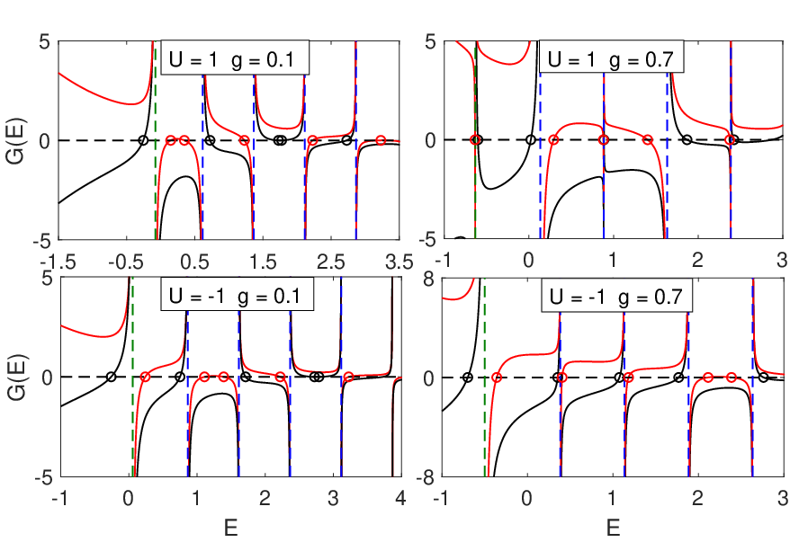
3.1 Pole structure
We first examine the pole structure of the -function (17). Note from Eq. (14) that the denominator of for vanishes, yielding the -th pole of the -function
| (18) |
It is interesting to find that this pole is reduced to , the pole of the pure QRM [45], if set .
From Eq. (13), one can find that diverges at
| (19) |
However it is not the pole of the -function, because appears always as a whole in the -function (17) and is finite at for .

3.2 Exceptional solutions
3.2.1 Juddian solutions for doubly degenerate states
If the true physical system takes the energy at the zeroth pole , the wavefunction (7) including terms should be analytic. Hence both the denominator and numerator of should vanish at the same time, yielding the constrained condition for the model parameter
| (21) |
Inserting Eq. (21) into Eq. (20) gives the energy without specified parity . The first energy levels for both parities thus intersect at . These are the doubly degenerate states, corresponding to the Juddian solution [53].
Physically, the energies for the ground-state and the first excited state cross, indicating a first-order quantum phase transition. According to Eq. (21), note that the qubit frequency is always positive, so the finite real only exists for . No first-order phase transition exists in the present model for and the linear QRM where . As shown in the upper panels of Fig. 2, two levels for the first excited state and ground state really cross once for . Such a crossing for the two lowest levels does not occur for , as shown in the lower panels.
Actually, for any , if both denominator and numerator of in Eq. (13) vanish, is analytic, leading to analytic coefficients and . The reason is the following. is analytic for both and . The denominator of in Eq. (14) is
we can easily find that both denominator and numerator of should be also zero, leading to analytic coefficients , and therefore analytic coefficients .
The condition that both the denominator and numerator of in Eq. (13) vanish will give the coupling strength
| (22) |
The corresponding energy , which is surprisingly independent of the coupling strength!
Similarly, the parity is not well defined at this energy. It is just the crossing point corresponding to doubly degenerate states. Because is also analytic at this point, the pole curves (18) should also pass through these crossing points. As demonstrated in Fig. 2 that all these crossing points for different (blue squares) just situate on a horizontal line in the energy spectra. They are usually the last crossing points for each pair of levels with positive and negative parity and somehow hardly discerned without analytical reasonings.
Interestingly we can give a lower bound for number of states below for given by counting the level crossing points. According to Eq. (22), we get maximum number for ,
| (23) |
where the bracket […] denotes the Gaussian step function. There are level crossings at the same energy in the coupling regime , as shown in Fig. 2. Note that those levels pass through crossing points will lie below at . Then for given , we find at least states below . In the limit , by Eq. (23). So at , there are possibly an infinite number of levels below or equal to for any .
All other Juddian solutions for doubly-degenerate states can be figured out in terms of the pole energy (18). It is required that the numerator of vanishes. For example, for pole,
and can be obtained through Eq. (13), and substitution to Eq. (14) yields
It requires numerator to be zero, i.e.
this is just the constrained condition. Therefore we can obtain several for pole curve in the energy spectra for fixed and .
The constrained condition becomes more complicated with larger , but in principle can be obtained. Proceeding along this line, we can predict the values of for fixed in the spectra for any . By the way, the largest for the crossing points obtained in this way should be the same as that in Eq. (22), as stated before. These predicted values coincide with the level crossing marked by blue filled circles and squares, as exhibited in Fig. 2.
3.2.2 Exceptional solution for nondegenerate states

As in the original QRM, it is possible that the -th pole line can cross the energy levels away from the level crossings, leading to exceptional solutions for the non-degenerate state [29]. With fixed , let and , the nondegenerate exceptional -function in space is defined as [54]
| (24) |
where the energy is limited to by Eq. (18). The zeros of exceptional -function (24) will give the coupling strength.
Particularly, for the zeroth pole, c. f. Eq. (20), the summation in the -function is then the same as in Eq. (17). Note however that in the first term diverges if using . In this case, we can start with in recurrence relation instead, so all coefficients are well defined, including due to . The nondegenerate exceptional -function is thus
| (25) |
We exhibit the nondegenerate -function as a function of for in Fig. 3 (a)-(d) for . The zeros give the coupling strength where the non-degenerate exceptional solution occurs, which are marked with green circles. To show the precise location of these nondegenerate exceptional solutions, we also calculate the energy spectra with the same parameters, which is displayed in Fig. 3 (e). The green circles for are also marked, which are just the zeros exhibited in Fig. 3 (a)-(d).
So far, the energy spectra of the quantum Rabi-Stark model for the regular type and two kinds of exceptional ones are completely obtained.
4 Spectral accumulation and collapse at
Note that the present -function (17) is not valid at , because in Eqs. (13) diverges. The spectral phenomena at should be studied in another way. We here present our analysis for by a new approach in detail. For the case of , the extension is achieved straightforwardly by changing into .
The bosonic components of Hamiltonian can be expressed in terms of the effective position and momentum operators of a particle of mass , defined as
| (26) |
for simplicity we can set . In terms of two eigenstates of , the Hamiltonian in the matrix form then takes
| (27) |
Suppose the wavefunction is , we have two coupled Schrödinger equations
Inserting to the first equation results in the effective one-body Hamiltonian for
where
| (28) |
with
One can easily find the eigenvalues of this quantum harmonic oscillator
| (29) |
To have the real harmonic frequency, should be positive, which results in or . For , we have the equation for the energy
| (30) |
while for , we have another equation for the energy
| (31) |
These two equations are exactly the same as Eqs. (39-41) [55] by Maciejewski et al. Our solution based on a harmonic oscillator is much simpler. It must be related to the fact that Maciejewski et al. uses the Bargmann space and transform the equations first into the so-called Birkhoff form, apparently creating unnecessary complications. They obtain also Hermite polynomials for the eigenfunctions in Bargmann space, but we would say that the Hermite polynomials are the wave-functions in the ordinary Hilbert space because the system is just a harmonic oscillator with shifted frequency.
From Eq. (31), we can see that an infinite number of discrete energy levels is confined in the energy interval
| (32) |
if . For convenience, we denote and . The effective potential becomes flat if , i.e. . In this case, there are qubit states which turn the potential flat [26, 56], and the spectrum collapses, like for a free particle. The infinite discrete energy levels in the low energy region for would collapse to for .

For , from Eqs. (31) and (32), we know that no real solutions exist in this case. Then we have to resort to numerics. In Fig. 4, we exhibit the first several energy levels for with different truncation of the Fock space by numerical exact diagonalziation. in this case. All energies for become closer to monotonously with increasing truncated photonic number , although the convergence is hardly achieved by numerics. It is observed that is a lower bound in the regime of . In the two-photon QRM [26, 27], it can be easily checked that the energy in numerical diagonalization has no a lower bound when coupling strength is larger than the half of cavity frequency. Although both models have a common feature of spectral collapse at a critical coupling, they display essentially different behaviour above the critical coupling.
While for , one can see from the left-hand-side of each plot in Fig. 4 that the converging energies for low excited states in the present model are easily obtained numerically, which can be also confirmed by the solution to Eq. (31). However, it is extremely difficult to obtain the converging energy level by direct exact diagonalizations when energy approaches to . Close to , there is a quasi-continuum of states with an infinite number of discrete states.
We can analyze the average photonic number in each eigenstates. According to the effective harmonic oscillator (28), we have the wavefunction in the -th energy level
| (33) |
where is the Hermite polynomial of degree . Then we can calculate straightforwardly, which is however very tedious and not shown here. When is approximately equal to
| (34) |
One can find from Eq. (34) that diverges if energy level approaches to . So it is almost impossible to use numerical exact diagonalziation to calculate correctly the energy level if very close to . If the numerical truncation of the Fock space is below , the results depend naturally on the truncation. This is a case where only an analytical treatment can give the correct answer.
The high energy levels for for arbitrary coupling can be easily obtained by Eq. (30) analytically. Our hypothesis for the exotic energy distribution for at is the following. For , by Eq. (31), we know that infinitely many discrete levels lie below accumulation point . Close to , there is a quasicontinuum of states. All states are normalizable. They collapse to right at . When all these energy levels could only stay in energy interval , but absolutely cannot be given by Eq. (31). The corresponding states should be unnormalizable. In this energy interval, it is unclear whether there is a continuum of non-noramlizable states, or this region is empty, which remains an open question. This issue obviously could not be addressed by any numerics and the above analytical theory in the framework of a harmonic oscillator, therefore other rigorous study should be called for.
5 Conclusion
In this work, we have derived the -function for the quantum Rabi-Stark model in a compact way by using the BOA. Zeros of the -function determine the regular spectrum. Two kinds of exceptional solutions are clarified and demonstrated. For the Juddian-type solution, the true level crossing occurs at the doubly degenerate states with both parities, which exclude the previous ”crossing” from the same parity. The first-order phase transition is detected analytically by the pole structure of -functions. The critical coupling strength of the phase transitions is obtained analytically. The exotic energy spectra at are analyzed within an effective quantum harmonic oscillator. Previous energy spectra by very complicated and cumbersome derivation can be very easily reproduced. Moreover, the energy spectral collapse can be attributed by the flat quadratic potential. Below the collapse critical coupling, there are infinite discrete energy levels below the collapse energy.
Both the first-order quantum phase transition and the spectral collapse can occur in the present model, and are lacking in the linear QRM. The spectral collapse also occurs in the two-photon QRM with another kind of nonlinear coupling, but the first-order quantum phase transition is absent. Spectral collapse does not occur in the anisotropic QRM where the first-order phase transitions can be induced by the anisotropy with respect to the rotating-wave and non-rotating-wave coupling strengths. It follows that the Stark-like nonlinear coupling between atom and cavity is of fundamental importance. We believe that the quantum Rabi-Stark model would exhibit various fundamental phenomena found in the various QRMs, and could even go beyond. The spectral collapse and the discrete levels below the collapse energy might be qualitatively understood in the polaron picture by the tunneling induced potential well [57]. Due to the parity symmetry, the second-order phase transition in the present model should also occur in the limit , like that in the linear QRM [58, 59, 60, 61]. We speculate that the present model would possibly experience true superradiance transition in the single-atom model at moderate frequency ration . Other peculiarities and novel properties in quantum Rabi-Stark model are also worthy of further explorations. The well understanding of the closed system will lay the solid foundation for further treatment of the open quantum system [62].
References
References
- [1] Braak D, Chen Q H, Batchelor M T and Solano E 2016 \jpa49 300301
- [2] Mabuchi H and Doherty A C 2002 Science 298 1372
- [3] Jaynes E T and Cummings F W 1963 Proc. IEEE 51 89
- [4] Scully M O and Zubairy M S 1997 Quantum Optics (Cambridge University Press, Cambridge) Orszag M 2008 Quantum Optics ((Heidelberg: Springer))
- [5] Niemczyk T et al 2010 Nature Physics 6 772
- [6] Forn-Díaz P et al 2010 Phys. Rev. Lett. 105 237001
- [7] Chen Z, Wang Y M, Li T F, Tian L, Qiu Y Y, Inomata K, Yoshihara F, Han S Y, Nori F, Tsai J S and You J Q 2017 Phys. Rev. A 96 012325
- [8] Yoshihara F, Fuse T, Ashhab S, Kakuyanagi K, Saito S and Semba K 2016 Nat. Phys. 13 44
- [9] Forn-Díaz P, García-Ripoll J J, Peropadre B, Orgiazzi J-L, Yurtalan M A, Belyansky R, Wilson C M and Lupascu A 2016 Nat. Phys. 13 39
- [10] Anappara A A, De Liberato S, Tredicucci A, Ciuti C, Biasiol G, Sorba L and Beltram F 2009 Phys. Rev. B 79 201303 Todorov Y, Andrews A M, Colombelli R, De Liberato S, Ciuti C, Klang P, Strasser G and Sirtori C 2010 Phys. Rev. Lett. 105 196402 Zhang Q, Lou M, Li X, Reno J L, Pan W, Watson J D, Manfra M J and Kono J 2016 Nat. Phys. 12 1005
- [11] Schneeweiss P, Dareau A and Sayrin C 2018 Phys. Rev. A 98 021801(R)
- [12] Casanova J, Romero G, Lizuain I, García-Ripoll J J and Solano E 2010 Phys. Rev. Lett. 105 263603
- [13] Werlang T et al 2008 Phys. Rev. A 78 053805
- [14] Zueco D et al 2009 Phys. Rev. A 80 033846
- [15] Ashhab S and Nori F 2010 Phys. Rev. A 81 042311
- [16] Hausinger J and Grifoni M 2010 Phys. Rev. A 82 062320
- [17] Chen Q H, Li L, Liu T and Wang K L 2012 Chin. Phys. Lett. 29 014208
- [18] Bayer A, Pozimski M, Schambeck S, et al. 2017 Nano Lett 17 6340-6344
- [19] Kockum A F, Miranowicz A, Liberato S D, Savasta S and Nori F 2019 Nat. Rev. Phys. 1 19
- [20] Puebla R, Hwang M-J, Casanova J and Plenio M B 2017 Phys. Rev. Lett. 118 073001 Felicetti S, Rico E, Sabin C, Ockenfels T, Koch J, Leder M, Grossert C, Weitz M and Solano E 2017 Phys. Rev. A 95 013827
- [21] Grimsmo A L and Parkins S 2013 Phys. Rev. A 87 033814
- [22] Grimsmo A L and Parkins S 2014 Phys. Rev. A 89 033802
- [23] Klimov A B and Chumakov S M 2009 A Group-Theoretical Approach to Quantum Optics-Models of Atom-Field Interactions (Weinheim: Wiley) page 106
- [24] Eckle H-P and Johannesson H 2017 \jpa50 294004
- [25] Ng K M, Lo C F and Liu K L 1999 Eur. Phys. J. D 6 119
- [26] Felicetti S, Pedernales J S, Egusquiza I L, Romero G, Lamata L, Braak D and Solano E 2015 Phys. Rev. A 92 033817
- [27] Duan L-W, Xie Y-F, Braak D and Chen Q H 2016 \jpa49 464002
- [28] Xie Q T, Cui S, Cao J P, Amico L and Fan H 2014 Phys. Rev. X 4 021046
- [29] Maciejewski A J, Przybylska M and Stachowiak T 2014 Phys.Lett. A 378 3445
- [30] Xie Q T, Zhong H H, Batchelor M T and Lee C H 2016 \jpa50 113001
- [31] Gu X, Kockum A F, Miranowicz A, Liu Y X and Nori F 2017 Physics Reports 718-719 1-102
- [32] Forn-Díaz P, Lamata L, Rico E, Kono J and Solano E arXiv:1804.09275
- [33] Swain S 1973 J. Phys. A: Math. Nucl. Gen. 6 1919
- [34] Kus M 1985 J. Math. Phys. 26 2792 Kus M and Lewenstein M 1986 J. Phys. A: Math. Gen. 19 305
- [35] Durstt C, Sigmundt E, Reineker P and Scheuing A 1986 J. Phys. C: Solid State Phys. 19 2701
- [36] Feranchuk I D, Komarov L I and Ulyanenkov A P 1996 J. Phys. A: Math. Gen. 29 4035
- [37] Bishop R F et al 1996 Phys. Rev. A 54 R4657 Bishop R F and Emary C 2001 J. Phys. A: Math. Gen. 34 5635 (2001).
- [38] Irish E K 2007 Phys. Rev. Lett. 99 173601
- [39] Paganelli S and Ciuchi S 2008 J. Phys.: Condens. Matter20 235203
- [40] Chen Q H, Yang Y, Liu T and Wang K L 2010 Phys. Rev. A 82 052306
- [41] Pan F, Guan X, Wang Y and Draayer J P 2010 J. Phys. B: At. Mol. Opt. Phys.43 175501
- [42] Chen Q H, Liu T, Zhang Y Y and Wang K L 2011 Europhys. Lett. 96 14003
- [43] Ying Z J, Liu M X, Luo H G, Lin H Q and You J Q 2015 Phys. Rev. A 92 053823
- [44] Zhang Y Y 2016 Phys. Rev. A 94 063824
- [45] Braak D 2011 Phys. Rev. Lett. 107 100401
- [46] Zhong H H, Xie Q T, Batchelor M T and Lee C H 2013 \jpa46 415302 Zhong H H, Xie Q T, Guan X W, Batchelor M T, Gao K and Lee C H 2014 \jpa47 045301
- [47] Chen Q H, Wang C, He S, Liu T and Wang K L 2012 Phys. Rev. A 86 023822
- [48] Villas-Boas C J and Daniel Z. Rossatto D Z 2019 Phys. Rev. Lett. 122 043601
- [49] Travěnec I 2012 Phys. Rev. A 85 043805
- [50] Cui S, Cao J P, Fan H and Amico L 2017 \jpa50 204001
- [51] Chen Q H, Zhang Y Y, Liu T and Wang K L 2008 Phys. Rev. A 78 051801(R)
- [52] Braak D 2013 Ann. Phys. (Berlin) 525, L23
- [53] Judd B R 1979 J. Phys. C 12 1685
- [54] Braak D 2015 Proc. Forum ‘Math-for-Industry 2014’ (New York: Springer)
- [55] Maciejewski A J, Przybylska M and Stachowiak T 2015 Phys.Lett. A 379 1503
- [56] Penna V, Raffa F A and Franzosi R 2018 \jpa51 045301
- [57] Cong L, Sun X M, Liu M X, Ying Z J and Luo H G 2019 Phys. Rev. A 99 013815
- [58] Hwang M-J, Puebla R and Plenio M B 2015 Phys. Rev. Lett. 115 180404
- [59] Liu M X, Chesi S, Ying Z J, Chen X S, Luo H G and Lin H Q 2017 Phys. Rev. Lett. 119 220601
- [60] Shen L T, Yang Z B, Wu H Z and Zheng S B 2017 Phys. Rev. A 95 013819
- [61] Ashhab S 2013 Phys. Rev. A 87 013826
- [62] Dimer F, Estienne B, Parkins A S and Carmichael H J 2007 Phys. Rev. A 75 013804 Baumann K, Guerlin C, Brennecke F and Esslinger T 2010 Nature (London) 464 1301 Keeling J, Bhaseen M J and Simons B D 2010 Phys. Rev. Lett. 105 043001 Kirton P, Roses M M, Keeling J and Dalla Torre E G 2018 Adv. Quantum Technol. 2 1800043.