Signs of Dynamical Dark Energy in Current Observations
Joan Solà Peracaula, Adrià Gómez-Valent and Javier de Cruz Pérez
Departament de Física Quàntica i Astrofísica, and Institute of Cosmos Sciences,
Universitat de Barcelona,
Av. Diagonal 647, E-08028 Barcelona, Catalonia, Spain
E-mails: sola@fqa.ub.edu, adriagova@fqa.ub.edu, decruz@fqa.ub.edu
Abstract. Investigations on dark energy (DE) are currently inconclusive about its time evolution. Hints of this possibility do however glow now and then in the horizon. Herein we assess the current status of dynamical dark energy (DDE) in the light of a large body of updated SNIa++BAO+LSS+CMB observations, using the full Planck 2015 CMB likelihood. The performance of the CDM model (with equation of state for ) is confronted with that of the general XCDM and CPL parametrizations, as well as with the traditional CDM model based on the scalar field potential . In particular, we gauge the impact of the bispectrum in the LSS and BAO parts, and show that the subset of CMB+BAO+LSS observations may contain the bulk of the DDE signal. The departure from is significant: roughly for XCDM and for CDM. In both cases the full Bayesian evidence is found to be positive even for a prior range of the DDE parameters extending over several standard deviations from the mean when the bispectrum is taken into account. Positive signs follow as well from the preliminary results of Planck 2018 data using the compressed CMB likelihood. As a bonus we also find that the -tension becomes reduced with DDE.
Keywords: cosmological parameters, dark energy, large-scale structure of universe
1 Introduction
Even if the existence proof of the DE is not iron-clad, the great majority of cosmologists are agreed that the universe is in accelerated expansion [1, 2, 3] and that some physical cause must be responsible for it. The canonical picture in GR is to assume that such cause is the presence of a cosmological constant (CC) term, , in Einstein’s equations. No reason, however, is given for its constancy throughout the entire cosmic history. In fact, const. is not required by the cosmological principle. Such oversimplification might be at the root of the Cosmological Constant Problem, namely the appalling discrepancy between the measured value of the vacuum energy density, GeV4 (G being Newton’s constant), and the incommensurably larger value predicted in quantum field theory (QFT) [4, 5, 6, 7]. The cosmological constant problem stays unsolved right now, even after more than a full century after was first introduced by Einstein. Most likely the mystery will remain for a long time still. In this work, we will not attempt to solve it. Our main aim is much more humble. Somehow we wish to follow the original phenomenological approach that made possible to unveil that is nonvanishing, irrespective of its ultimate physical nature. The method to substantiate that is non-null was largely empirical, namely was assumed to be a parameter and then fitted directly to the data. Of course a minimal set of assumptions had to be made, such as the validity of the Cosmological Principle and hence of the Friedmann-Lemaître-Robertson-Walker (FLRW) metric, with the ensuing set of Friedmann equations for the scale factor. In our case, we wish of course to keep these minimal assumptions and make a phenomenological case study of the next-to-leading possibility, which is that the , or in general the DE, might be not just a parameter but a slowly varying cosmic variable that stays close to a constant for cosmic spans of time and therefore capable of mimicking the CDM-like behavior.
This is all the most interesting if we take into account that, aside from theoretical problems, a number of persisting tensions with the data (particularly on the local value of the Hubble parameter [8, 9] and the large scale structure formation data [10]) suggest that the concordance or CDM model, with rigid -term, might be performing insufficiently at the observational level. The possibility to alleviate some of these problems by assuming that , or in general the DE, might be (slowly) dynamical is a natural option to test, see e.g. [11, 12, 13]. Here we are primarily spurred by these phenomenological considerations and the disparity of different results. For instance, hints of DDE were highlighted in [14, 15, 16]. In addition, nonparametric studies of the DDE suggest positive evidence at about c.l., see [17]. Such confidence level is actually comparable to that achieved through specific models of DDE, in which attempts were made to cure the mentioned tensions – see e.g. [18, 19, 20, 21] and references therein. Other recent works, in contrast, find a variety of levels of evidence in different contexts or simply no sizeable deviation from the CDM, see [22, 23, 24, 25, 26, 27, 28, 29, 30, 31, 32, 33, 34] and references therein, for example.
In this paper, we reassess the current situation on the DDE and try to clarify why some authors find evidence whereas others find no evidence at all. The novelty is that we pay due attention to the sensitivity of the signal to potentially relevant features sitting in the baryon acoustic oscillations (BAO) and large-scale structure (LSS) formation data which have not been explored in previous studies. Most noticeably we explore the inclusion of the matter bispectrum together with the power spectrum. We find that this ingredient helps to develop more sensitivity to the DDE signal. We test and confirm this fact by considering the reaction of well-known generic parametrizations of the DDE, such as the XCDM and CPL, as well as a well-known representative of the traditional class of scalar field models (CDM). Our analysis is performed on the basis of a large set of updated SNIa++BAO+LSS+CMB observations and leads to a signal of DDE in the ballpark of c.l. Such positive test is encouraging. If revalidated with the advent of future data, it could guide us into future strategies helping to consolidate the DDE signature.
| DS1 with Spectrum (DS1/SP) | DS1 with Bispectrum (DS1/BSP) | ||||||
| Parameter | CDM | XCDM | CDM | CDM | XCDM | CPL | CDM |
| (km/s/Mpc) | |||||||
| -1 | - | -1 | - | ||||
| - | - | - | - | - | - | ||
| - | - | - | - | - | , | ||
2 DDE parametrizations and models
We consider two generic parametrizations of the DDE, together with a well-known CDM model, and confront them to a large and updated set of SNIa++BAO+LSS+CMB observations. Natural units are used hereafter, although we keep explicitly Newton’s , or equivalently the Planck mass: GeV. Flat FLRW metric is assumed throughout: , where is the scale factor as a function of the cosmic time.
2.1 XCDM and CPL
The first of the DDE parametrizations under study is the conventional XCDM [35]. In it both matter and DE are self-conserved (non-interacting) and the DE density is simply given by , where is the current value and the (constant) equation of state (EoS) parameter of the DE fluid. For we recover the CDM model with a rigid CC. For the XCDM mimics quintessence, whereas for it mimics phantom DE. It is worth checking if a dynamical EoS for the DE can furnish a better description of the observational data. So we consider the well-known CPL parametrization [36, 37], which is characterized by the following EoS:
| DS2 with Bispectrum (DS2/BSP) | DS2/BSP with Planck 2018 (compressed likelihood) | |||||
| Parameter | CDM | XCDM | CDM | CDM | XCDM | CDM |
| (km/s/Mpc) | ||||||
| - | - | - | ||||
| -1 | - | -1 | - | |||
| - | - | , | - | - | , | |
| (1) |
where is the cosmological redshift. The corresponding Hubble rate normalized with respect to the current value, , takes the form:
| (2) |
Here are the current energy densities of baryons, cold dark matter, photons and CC/DE normalized with respect to the present critical density . The neutrino contribution, is more complicated since it contains a massive component, , apart from the massless ones. During the expansion of the universe, the massive neutrino transits from a relativistic to a nonrelativistic regime. This process is nontrivial and has to be solved numerically. In the above expression, for we recover the XCDM, and also setting we are back to the CDM.

2.2 CDM
Let us now briefly summarize the theoretical framework of the CDM, which has a well-defined local Lagrangian description. The DE is described here in terms of a scalar field, , which we take dimensionless. Such field is minimally coupled to curvature () and the generic action is just the sum of the Einstein-Hilbert action , the scalar field action , and the matter action :
| (3) |
The energy density and pressure of follow from its energy-momentum tensor, , and the fact that is a homogeneous scalar field which depends only on the cosmic time. Thus,
| (4) |
Dots indicate derivatives with respect to the cosmic time, and notice that within our conventions has dimension 2 in natural units.
The field equation for is just the Klein-Gordon equation in curved spacetime, , which for the FLRW metric leads to
| (5) |
The corresponding Einstein’s field equations read:
| (6) | |||
| (7) |
Here involves the pressureless contributions from baryons and cold dark matter as well as the massive neutrino contribution. The latter evolves during the cosmic expansion from the relativistic regime (where ) to the nonrelativistic one (where ). On the other hand, is the purely relativistic part from photons and the massless neutrinos.

As a representative potential for our analysis we borrow the traditional quintessence potential by Peebles and Ratra [38, 39],
| (8) |
where is a dimensionless parameter. In this context, the value of the CC at present () is given by . We expect to be positive since we know that and the potential energy at present is dominant. In what follows, when referring to the CDM model we will implicitly assume this form of the potential. The power in it should be positive as well, but sufficiently small so that mimics an approximate CC slowly evolving with time. In our case we take as a free parameter while is a derived one, as discussed below.
The Klein-Gordon equation with the potential (8) can be written in terms of the scale factor as follows (prime stands for , and we use ):
| (9) |
When the cosmic evolution is characterized by the dominant energy density ( for the matter-dominated epoch and for radiation-dominated), i.e. when the DE density is negligible, one can search for power-law solutions of the Klein-Gordon equation, i.e. solutions of the form . However, around the current time the effect of the potential is significant and the solution has to be computed numerically. Equation (9) is coupled to the cosmological equations under appropriate initial conditions. We can set these conditions at the radiation epoch, where we can neglect the DE. We find
| (10) |
Notice that is the total radiation energy density, which includes also the massive neutrino contribution. At the radiation epoch, however, behaves very approximately as . Thus, Eq.(10) together with obtained from it can be used for the numerical solution of Eq. (9) and of the EoS of the scalar field at any subsequent epoch: .
To compare the theoretical predictions of the different models under study with the available observational data we have made use of the Einstein-Boltzmann code CLASS [41] in combination with the powerful Monte Carlo Markov chain (MCMC) sampler MontePython [42]. In the particular instance of CDM, we have conveniently modified CLASS such as to implement the shooting method, see [43] for a detailed exposition, what allowed us to consistently determine the value of for each value of the free parameter . As it is well-known, such numerical technique consists in replacing a boundary value problem with an initial value one through a large number of iterations of the initial conditions until finding the optimized solution. For the CDM, the initial conditions are determined by (10) and its time derivative, which are both explicitly dependent on .
3 Data
The main fitting results of our analysis are presented in Tables 1 and 2. An additional Table 3 has also been introduced to illustrate the correct normalization of our results with other existing studies in the literature when we use comparable data. This issue will be further discussed throughout our presentation. To generate the fitting results displayed in Tables 1, 2 and 3 we have run the MCMC code MontePython, together with CLASS, over an updated data set SNIa++BAO+LSS+CMB, consisting of: i) 6 effective points on the normalized Hubble rate (including the covariance matrix) from the Pantheon+MCT sample [44, 45], which includes 1063 SNIa. As it is explained in [45], the compression effectiveness of the information contained in such SNIa sample is extremely good; ii) 31 data from from cosmic chronometers [46, 47, 48, 49, 53, 50, 51, 52]; iii) 16 effective BAO points [55, 56, 57, 54, 58]; iv) 19 effective points from LSS, specifically 18 points from the observable (obtained from redshift-space distortions – RSD) [66, 67, 64, 60, 63, 62, 68, 56, 59, 61, 58, 65] and one effective point from the weak lensing observable [69]; v) Finally we make use of the full CMB likelihood from Planck 2015 TT+lowP+lensing [3]. It is important to emphasize that we take into account all the known correlations among data. Owing to their special significance in this kind of analysis, we have collected the set of BAO and LSS data points used in this work in the Tables 4 and 5, respectively.
The total data set just described will be referred to as DS1. This is our baseline scenario since it involves a large sample of all sorts of cosmologial data and will be used to compare with the possible additional effects that emerge when we enrich its structure, as we shall comment in a moment. For a more detailed discussion of the data involved in DS1, see [12, 16, 21]. In this study, however, we wish to isolate also the effect from the triad of BAO+LSS+CMB data. These ingredients may be particularly sensitive to the DDE, as shown in the previous references. Such subset of DS1 will be called DS2 and contains the same data as DS1 except SNIa+. In the next section we define further specifications of these two datasets with special properties.
| Survey | Observable | Measurement | References | Data set | |
| 6dFGS+SDSS MGS | [Mpc] | [Mpc] | [54] | SP/BSP | |
| WiggleZ | [Mpc] | [Mpc] | [55] | SP/BSP | |
| [Mpc] | [Mpc] | ||||
| [Mpc] | [Mpc] | ||||
| DR12 BOSS (BSP) | [56] | BSP | |||
| DR12 BOSS (SP) | [Mpc] | [72] | SP | ||
| [km/s/Mpc] | |||||
| [Mpc] | |||||
| [km/s/Mpc] | |||||
| [Mpc] | |||||
| [km/s/Mpc] | |||||
| eBOSS | [58] | SP/BSP | |||
| Ly-forest | [57] | SP/BSP | |||
| Survey | References | Data set | ||
|---|---|---|---|---|
| 2MTF | [59] | SP/BSP | ||
| 6dFGS | [60] | SP/BSP | ||
| SDSS-DR7 | [61] | SP/BSP | ||
| GAMA | [62] | SP/BSP | ||
| [63] | ||||
| DR12 BOSS (BSP) | [56] | BSP | ||
| DR12 BOSS (SP) | [72] | SP | ||
| WiggleZ | [64] | SP/BSP | ||
| VIPERS | [65] | SP/BSP | ||
| VVDS | [66],[67] | SP/BSP | ||
| FastSound | [68] | SP/BSP | ||
| eBOSS | [58] | SP/BSP | ||
4 Spectrum versus bispectrum
The usual analyses of structure formation data in the literature are performed in terms of the matter power spectrum , referred to here simply as spectrum (SP). As we know, the latter is defined in terms of the two-point correlator of the density field in Fourier space, namely , in which is the Dirac delta of momenta. For a purely Gaussian distribution, any higher order correlator of even order decomposes into sums of products of two-point functions, in a manner very similar to Wick’s theorem in QFT. At the same time, all correlators of odd order vanish. This ceases to be true for non-Gaussian distributions, and the first nonvanishing correlator is then the bispectrum , which is formally connected to the three-point function
| (11) |
The Dirac selects in this case all the triangular configurations. Let us note that even if the primeval spectrum would be purely Gaussian, gravity makes fluctuations evolve non-Gaussian. Such deviations with respect to a normal distribution may be due both to the evolution of gravitational instabilities that are amplified from the initial perturbations, or even from some intrinsic non-Gaussianity of the primordial spectrum. For example, certain implementations of inflation (typically multifield inflation models) unavoidably lead to a certain degree of non-Gaussianity [70]. Therefore, in practice the bispectrum is expected to be a nonzero parameter in real cosmology, even if starting from perfect Gaussianity, which is in no way an absolute condition to be preserved. On the other hand, such departure should, of course, be small. But the dynamics of the DE is also expected to be small, so there is a possible naturalness relationship between the two.
The bispectrum (BSP) has been described in many places in the literature, see e.g. [70, 71] and references therein. The physical importance of including the bispectrum cannot be overemphasized as it furnishes important complementary information that goes beyond the spectrum. If fluctuations in the structure formation were strictly Gaussian, their full statistical description would be contained in the two-point correlation function since, as already mentioned, all higher order correlators of even order can be expanded in terms of products of two-point functions. In such a case the formal bispectrum defined above would identically vanish. However, there is no a priori reason for that to happen, and in general this is not what we expect if we take into consideration the reasons mentioned above. The crucial question is: how to test the real situation in practice? While the above definitions are the formal ones, operationally (in other words, at the practical level of galaxy counting) one must resort to use SP and BSP estimators of empirical nature. For the power spectrum estimator one may use , where is the Fourier transform of an appropriately defined weighted field of density fluctuations, that is to say, one formulated in terms of the number density of galaxies [56].
Similarly, a bispectrum estimator can be defined from the angle-average of closed triangles defined by the -modes, , where is the Fourier transform of the corresponding weighted field of density fluctuations defined in terms of the number density of galaxies. It can be conveniently written as
| (12) |
i.e. through an expression involving a separate product of Fourier integrals
| (13) |
Here is the fundamental frequency, , the size of the box in which the galaxies are embedded and
| (14) |
is the number of fundamental triangles inside the shell defined by , and , with the region of the -modes contained in a -bin, , around . The Dirac insures that only closed triangles are included – see the mentioned references for more details. The measurement of the bispectrum estimator is essential to be sensitive to possible higher order effects associated to non-Gaussianities in the distribution of galaxies. This task is what has been done in the important work [56].
Here we wish to dwell on the impact of the bispectrum as a potential tracer of the DDE. Observationally, the data on BAO+ LSS (more specifically, the part of LSS) including both the spectrum (SP) and bispectrum (BSP) are taken from [56], together with the correlations among these data encoded in the provided covariance matrices. The same data including SP but no BSP has been considered in [72]. In this study, we analyze the full dataset DS1 with spectrum only (dubbed DS1/SP) and also the same data when we include both SP and BSP (denoted DS1/BSP for short). In addition, we test the DDE sensitivity of the special subset DS2, which involves both SP+BSP components (scenario DS2/BSP). The contrast of results between the “bispectrumless” scenarios (i.e. the pure SP ones) and those including the matter bispectrum component as well (i.e. the SP+BSP ones) will be made apparent in our study, specially through our devoted discussions in sections 5 and 6.
The numerical fitting results that we have obtained for the DDE models under examination and the CDM are displayed in Tables 1 and 2. While we use Planck 2015 CMB data with full likelihood throughout most of our analysis, in the second block of Table 2 we report on the preliminary results obtained from the recent Planck 2018 CMB data under compressed likelihood [78, 79]. Let us note that the full likelihood for Planck 2018 CMB data is not public yet. We discuss the results that we have obtained and their possible implications in the next two sections.
As indicated above, an additional fitting table has been generated (Table 3) in order to illustrate the fact that the results presented in our work are consistent with other studies presented in the literature, namely for the case when we restrict our analysis to the baseline bispectrumless scenario introduced in our work (i.e. DS1/SP). We substantiate this fact by introducing an alternative bispectrumless scenario, which we call DS3/SP. The latter is essentially coincident with the one used in the investigations of the same models recently presented by the authors of [28, 29], although there exist some mild differences between our DS3/SP scenario and the one considered by these authors, to wit: (i) In the supernovae sector there appear two differences: first, we use the compressed Pantheon+MCT data [44] mentioned in the previous section, which in expanded form includes more than one thousand supernovae, whereas they use the full (uncompressed) list of supernova data from the Pantheon compilation, but in their list – and here lies the second difference– they do not include the 15 high-redshift SNIa () from the CANDELS and CLASH Multy-Cycle Treasury (MCT) programs. However these differences should not be significant at all, and we refer the reader to the detailed discussion in Ref. [45] to justify why is so. In fact, in the latter reference it is demonstrated that the constraints derived from the full Pantheon+MCT compilation of supernovae of Type Ia are essentially indistinguishable from those derived from the corresponding compressed likelihood (see Fig. 3 of that reference); (ii) Concerning the BOSS Ly-forest data, they use the exact distributions, whereas we use the Gaussian approximations. A direct comparison of the values of the fitting parameters reported in [28, 29] with those presented in our Table 3 confirms a high degree of compatibility, being the discrepancies in all cases a small fraction of . For instance, for the XCDM we obtain , and the authors of [28] find , which differs by less than from the former, taking the errors in quadrature. The difference with respect to the value of corresponding to the DS1/SP dataset in Table 1 is also small: . On these grounds we judge that the approach adopted in our analysis is fully consistent and that the tiny differences which may appear between the exact and compressed treatment of the SNIa and the exact and Gaussian Ly-forest likelihoods cannot be held responsible for any significant change in the main conclusions of our work as to the dynamical nature of the DE. Put another way, the preliminary signal of DDE that we find in this work cannot be attributed to the tiny differences among the bispectrumless data sets existing in the literature, whether our DS1/SP, DS3/SP, the exact one used e.g. by [28, 29] or any other consistent dataset employed by different authors. All these bispectrumless scenarios are statistically equivalent since they involve a sufficiently complete and uncorrelated set of data from the various SNIa++BAO+LSS+CMB sources and therefore they are mutually consistent within a fraction of errors. We must conclude that the emerging indications of DDE that we have encountered should rather originate from the peculiarities of the bispectrum component, which seems to be particularly sensitive to the dynamical features presumably sitting in the DE.

5 Confronting DDE to observations
As we can see from Tables 1 and 2, the comparison of the CDM with the DDE models points to a different sensibility of the data sets used to the dynamics of the DE. If we start focusing on the results from the bispectrumless scenario DS1/SP – cf. left block of Table 1 – there is no evidence that the DDE models perform better than the CDM. The XCDM, for instance, yields a weak signal which is compatible with (i.e. a rigid CC). This is consistent e.g. with the analysis of [28]. The CDM model remains also inconclusive under the same data. The upper bound of at ( at 2) recorded in that table is consistent, too, with the recent studies of [29]. The same conclusion is derived upon inspection of Table 3, based on the alternative bispectrumless scenario DS3/SP, whose fitting results are indeed consistent with those collected for our DS1/SP as well as with those from the mentioned references [28] and [29].
Notwithstanding, both the XCDM parametrization and the CDM model fare significantly better than the CDM if we consider the dataset DS1/BSP, i.e. upon including the bispectrum component of the BAO+LSS data. The corresponding DDE signature is about c.l. However, it is further enhanced within the restricted DS2/BSP dataset, where the XCDM and the CDM reach in between c.l. (cf. left block of Table 2). As for the CPL parametrization, Eq. (1), we record it explicitly in Table 1 for the DS1/BSP case only. One can check that even in this case the errors in the EoS parameters are still too big to capture any clear sign of DE dynamics, owing to the additional parameter present in this model. Specifically, we find and , hence fully compatible with a rigid CC ().
In Fig. 1 we show the contour plots in the and planes for the XCDM and CDM models, respectively, at different confidence levels, which are obtained with the (bispectrumless) DS1/SP data set. It is obvious from these contours that the models do not exhibit a clear preference for DDE. The contour plots for the XCDM (on the left side of Fig. 1) appear located roughly up and down with respect to the cosmological constant divide , and therefore we cannot appraise any marked preference for a deviation into the quintessence () or the phantom region (). Similarly, the contour plots for the parameter of the CDM model (indicated on the right side of Fig. 1) show that is consistent with zero at , which means that the potential (8) is perfectly compatible with a cosmological constant.

In Fig. 2, however, the situation has changed in a rather conspicuous way. Once more we display the corresponding contour plots for the XCDM and CDM models, but now they are obtained in the presence of the bispectrum, specifically we use in this case the DS2/BSP data set. While we could use the entire DS1/BSP set, the former subset (made exclusively on BAO+LSS+CMB) is slightly more sensitive and we choose it to illustrate which data tend to optimize the DDE signal. After all not all data is expected to be equally sensitive, and this is something that has already been noted for other DDE models [21]. Coming back to Fig. 2 we can see that, in stark contrast with Fig. 1, there is a marked preference for the contours of the XCDM to shift upwards into the quintessence region. Specifically, the EoS parameter lies now more than away from in the quintessence domain . On the other hand, in the CDM case (shown in the right plot of the same figure) we consistently find at a similar (actually slightly higher) c.l.

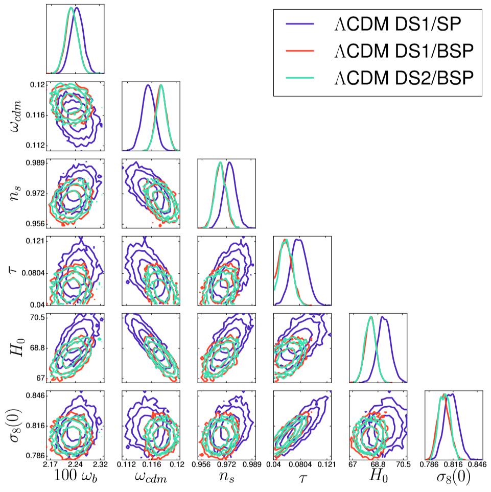
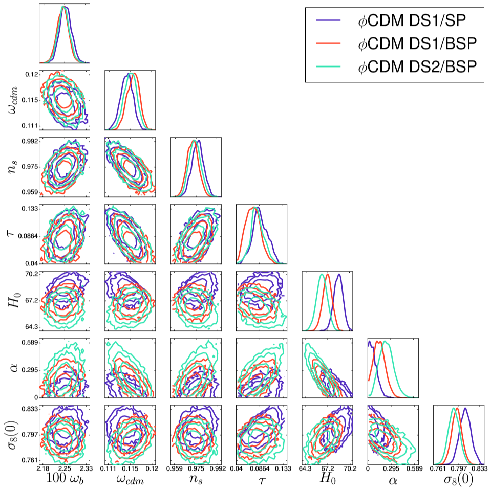
Figures 3-5 are also very illustrative. They contain the confidence contours in all the relevant planes of the parameter space up to c.l., together with the marginalized one-dimensional posterior distributions for the various fitting parameters. In Fig. 3 we present the results obtained with the DS1/SP, DS1/BSP and DS2/BSP scenarios in the context of the CDM. Figs. 4 and 5 contain the analogous plots for the XCDM and CDM, respectively. These figures allow us to appreciate in a very straightforward way what are the shifts in the confidence regions caused by the various changes of our cosmological data sets. Fig. 3 shows, for instance, that in the CDM the central values of all the parameters that enter the fit get shifted away from their DS1/SP values when the bispectrum information is also taken into account. These shifts are specially important for the parameters , , and , which in the DS1/BSP scenario are shifted , , and away with respect to the DS1/SP case. In contrast, and are lesser modified ( and , respectively). The removal of the SNIa+ data points from the DS1/BSP data set (which gives rise to the DS2/BSP one) does not produce any additional significant change in the CDM, as it can be easily checked by comparing the DS1/BSP and DS2/BSP contours and the corresponding one-dimensional distributions of Fig. 3. In the DDE models the effect on the parameters introduced by the bispectrum signal is quite different. To begin with, the values of , , and remain very stable and completely compatible at regardless of the data set under consideration. Moreover, the values of these parameters are also compatible with those of the CDM in the DS1/SP scenario. This means that the bispectrum does not force in the XCDM and CDM any important shift of the central values of , , and with respect to the typical values found in the CDM when we only consider the matter power spectrum part of the LSS+BAO data sector. Conversely, when we move from the DS1/SP scenario to the DS1/BSP and, finally, to the DS2/BSP, we find a progressive and non-negligible displacement of the peaks of the one-dimensional distributions for and towards lower values, which is accompanied by a departure of the DDE parameters of the XCDM () and CDM () from the CDM values ( and , respectively). The global decrease of from DS1/SP to DS2/BSP is () for XCDM (CDM), and the one of is for both models. This fact allows to reduce the well-known -tension [10] in a more efficient way in the context of the DDE models. However, the low values of the Hubble parameter derived in the XCDM and CDM from our fitting analyses keep the statistical tension with the local distance ladder determinations of [8, 9] high, reaching the latter the level. Nevertheless, it is important to remark that the values of obtained by us in the current study are perfectly consistent with those obtained by some authors that apply model-independent reconstruction techniques and low-redshift data from SNIa, BAO and data points from cosmic chronometers, see e.g. [73, 74, 75, 76, 77]. In the DDE scenarios analyzed in this paper, the -tension is directly linked with the -tension. We can only loosen the former at the expense of keeping the latter (cf. the contour lines in the - plane of Figs. 4 and 5). This is consistent with our analysis of [12], in which we studied other DDE models pointing to the same conclusion. Future data might be able to elucidate the ultimate origin of the -tension. If the true value of lies in the Planck-preferred region of km/s/Mpc, then the DDE models can offer an efficient way of automatically relieving the -tension.

From a more prospective point of view, in Figs. 6 and 7 we perform a preliminary exploration of the corresponding results using Planck 2018 data. The results for the same DDE models are obtained under different data set combinations, but on this occasion making use of the Planck 2018 compressed CMB data, given the mentioned fact that the full likelihood for Planck 2018 is not publicly available yet. These plots make, once more, palpable the importance of the bispectrum for the study of the DDE. Indeed, it is only when the bispectrum is included in the analysis, together with the CMB and BAO data sets, that a non-negligible signal in favor of the dynamical nature of the DE clearly pops out.
In Fig. 8 we plot the EoS of the various models in terms of the redshift near our time and within the error bands for the XCDM and CDM, again for the DS2/BSP case. These bands have been computed from a Monte Carlo sampling of the distributions. The behavior of the curves shows that the quintessence-like behavior is sustained until the present epoch. For the CDM we find , thus implying a DDE signal at c.l., which is consistent with the XCDM result11 1 We point out that the higher c.l. reported in [40] for these models originated from the unexpected change in the reported errors of the LSS data between the original version of [56] (i.e. their version v1) as compared to the published version (v2), in which the errors are slightly bigger..
Finally, in Fig. 9 we compute the matter power spectrum and the temperature anisotropies for the DDE models using Planck 2015 data, and also display the percentage differences with respect to the CDM. As can be seen, the differences of the CMB anisotropies between the DDE models and the CDM remain safely small, of order at most for the entire range. The suppression of the matter power spectrum of the DDE models in the relevant range of wave numbers with respect to the one of the concordance model is what gives rise to lower values of (cf. Tables 1-3).

6 Bayesian evidence of DDE
The main results of this work are synthesized in Tables 1 and 2, and in Figs. 1-10. Here we wish to quantify the significance of these results from the statistical point of view. This is done in detail in Fig. 10. In what follows we explain the meaning of this figure and review some basic facts on Bayesian analysis which can be helpful at this point. As remarked before, in the absence of BSP data the DDE signs are weak and we find consistency with previous studies. However, when we include BSP data and focus on the LSS+BAO+CMB observables (i.e. scenario DS2/BSP) the situation changes significantly. Both models XCDM and CDM then consistently point to a effect. Specifically, the evolving EoS of the CDM takes a value at present which lies away from the CDM () into the quintessence region (cf. Fig. 8). The significance of these results can be further appraised by computing the Bayesian evidence, which is based on evaluating the posterior probability of a model given the data and the priors, see e.g. [71, 80]. The relevant quantity we are looking for is the so-called Bayes factor, which does not depend on the arbitrarily assigned prior probability to the given model . If is the set of free parameters of such model, Bayes theorem allows us to compute the probability of measuring a distribution of values of these parameters given the measured dataset and the model . It is called the posterior probability, and it is given by
| (15) |
In words, it says that the posterior probability of is equal to the probability of the data given the parameters of the model (i.e. the likelihood ) times the prior probability of , , divided by the probability of the data (usually in the form of a probability distribution function, PDF). Obviously the latter does not depend on the values of . Therefore, if we normalize the posterior probability to one and integrate over all the parameters on both sides of Eq. (15), the corresponding integral in the numerator on the r.h.s. must be equal to :
| (16) |
This likelihood integral over all the values that can take the parameters is called the marginal likelihood or evidence [71, 80].
An analogous formula to (15) can also be applied to estimate the posterior probability that a model is true given a measured data set . Thus, following the same scheme, the posterior probability of the model given the data, , must be equal to the probability of the data given the model (irrespective of the values of ) – i.e. the marginal likelihood (16) — times the prior probability of the model, divided by the PDF of the data. Writing this relation for two cosmological models and that are being compared, we find that the ratio of posterior probabilities of these models is equal to the ratio of model priors times a factor:
| (17) |
Such factor, , is the so-called Bayes factor of the model with respect to model . It gives the ratio of marginal likelihoods (i.e. of evidences) of the two models. Note that it coincides with the ratio of posterior probabilities of the models only if the prior probabilities of these models are the same. This is generally assumed (“Principle of Insufficient Reason”) and hence the comparison of the two models and is usually performed directly in terms of .
In the literature it has been customary to define the Bayes information criterion (BIC) through the parameter , where is the minimum of , is the number of independent fitting parameters and is the total number of data points. One can show that the Bayes factor can be estimated through where is the difference between the values of BIC for models and [81, 82], i.e.
| (18) |
| Bayesian evidence of model versus | |
|---|---|
| weak evidence (consistency between both models) | |
| positive evidence | |
| strong evidence | |
| very strong evidence | |
| counter-evidence against model |
where is the difference between the minimum values of for each model, and is the difference in the number of independent fitting parameters of and , both describing the same data points. The added term to , i.e. , represents the penalty assigned to the model having the largest number of parameters (). Indeed, if has less parameters than (i.e. ) we expect that and hence . However, since the last term of (18) indeed penalizes the model with more parameters and compensates in part for its (presumably smaller) value of . Defined in this way, a positive value of the expression (18) denotes that the model is better than model , and the larger is the better is as compared to . Clearly, the Bayesian criterion allows a quantitatively implementation of Occam’s razor.
Even though the simple and very economic formula (18) is useful and has been applied in many places of the literature, see e.g. [18, 19, 20, 21] and references therein, it is only an approximate formula. The exact value of associated to the full Bayes factor requires to evaluate
| (19) |
where and are the two sets of free parameters integrated over for each model. We refer to this (exact) value of as the full “Bayesian evidence” of model versus model . It represents the optimal implementation of Occam’s razor. Formula (18) provides an estimate (sometimes good, sometimes rough) of the cumbersome expression (19). The evaluation of the latter is carried out in practice using the MCMC’s for the statistical analysis of the model and it can be a formidable numerical task. Fortunately it can be speeded up with the help of the recent numerical code MCEvidence [83]22 2 We thank Y. Fantaye for helpful advice in the use of the numerical package MCEvidence.. In Table 6 we collect the ranges of values of that are conventionally used in the literature to quantify the observational support of a given model with respect to some reference one [81, 82]. Consistently with the approximate formula discussed above, positive values of in the indicated intervals favor the model over model . In the situation under consideration is the CDM and is any of the considered DDE models. Small positive values near one just denote that the two models under competition are comparable (i.e. that there is no marked preference of over ), but larger and positive values of increase the support of (DDE model) versus (CDM). Negative values of , in contrast, would lead to the opposite conclusion, i.e. that the DDE model is penalized as compared to the CDM and hence that the latter is preferred.

In Fig. 10 we compute the full Bayesian evidence curves as a function of the prior range. We assume flat priors for the parameters in each model (we have no reason to assume otherwise). Thus is constant and cancels out for all common in the two models, rendering a pure ratio of marginal likelihoods. We define the unit of measure of the prior range, , as half the sum of the upper and lower fitting errors of the DDE parameters in Tables 1 and 2. In Fig. 10 we rate the level of support of the DDE models as compared to the CDM for each value of the prior range, following the standard definitions collected in Table 6 [81, 82].
As indicated, we utilized the code MCEvidence [83] to compute the exact values in Fig. 10. We have actually compared these results with those obtained for the evidences computed with Gaussian (Fisher) likelihoods for the parameters and we have found that they are qualitatively similar but with non-negligible numerical differences. These were expected from the mild departures of Gaussianity from the exact distributions. The full evidence curves in Fig. 10 reconfirm the mentioned result that with the bispectrumless dataset DS1/SP the evidence is weak. But at the same time we can recognize once more the impact of the bispectrum in the scenarios enriched with this component. Thus, it is remarkable to find a long tail of sustained positive Bayesian evidence both for the XCDM and CDM within the scenario DS2/BSP, which corroborates the higher sensitivity of the BAO+LSS+CMB data to DDE. The fact that with the full Planck 2015 data and with traditional models and parametrizations of the DE we can reach such significant level of evidence is encouraging. Even more reassuring is the fact that with the preliminary Planck 2018 data we can reach similar levels of evidence (cf. Table 2, second block, and also Figs. 6 and 7), which will have to be refined when the full Planck 2018 likelihood will be made public.
Last, but not least, let us emphasize one final important point of our analysis. Our results with BSP data show that the DDE values of (specially within the DS2/BSP scenario) are smaller than the (bispectrumless) CDM value quoted in Table 1 by roughly , thus essentially mitigating the -tension [10]. As remarked in Sect. 5 (related to our discussion on Fig. 3), the CDM value of does also diminish with BSP, but it is insufficient to alleviate the -tension. The latter is defined of course by taking as a reference the bispectrumless CDM result since the higher order corrections to the spectrum were never considered in previous analyses of the -tension. This is the reason why we have compared with that value in order to judge the performance of the DDE models in connection to such tension. We have checked also the influence of massive neutrinos. We find that a similar effect is possible within the CDM (under DS1/BSP) for a sum of neutrinos masses of eV, leading to . Recall, however, that in all our fitting tables we have included a light massive neutrino of eV, which is the standard assumption adopted in most analyses [3] so as to preserve the so-called normal hierarchy of neutrino masses (as required from neutrino oscillation experiments). A solution solely based on invoking a substantially massive neutrino scenario is thus ruled out since it clashes with the usual constraints on neutrino oscillations; specifically, it requires unnatural fine-tuning among the neutrino masses. The DDE option is, therefore, more natural. There may be, of course, other factors that could have an influence on this analysis, such as e.g. the possible concurrence of spatial curvature effects. When curvature is allowed to be a free parameter the constraints on DE dynamics may weaken since we then have an additional parameter. We have already seen a weakening of DDE evidence in the case of the CPL as compared to the XCDM, owing to the presence of one more parameter in the former case as compared to the latter. The effects of curvature in this kind of analyses have been studied for the main models under consideration in [27, 28, 29, 30, 31], and previously in [26, 84]. For instance, in [27] (see also references therein) the authors show that in the non-flat CDM model the spatial curvature also allows a decrease of the central value of when only the TT+lowP+lensing Planck 2015 CMB data is employed in the fitting analysis. When a more complete data set including SNIa++BAO+LSS is considered, though, such decrease is less significant. The same pattern is found e.g. for the CDM in [29]. It is nonetheless important to point out that the effect of the bispectrum signal in the BAO+LSS data sector has not been studied in the context of a spatially curved universe yet. It would be interesting to carefully assess it. Here, however, we have chosen to present our main results by placing emphasis on the impact of the bispectrum on the study of the DDE within the simplest possible scenario, which is to assume spatially flat FLRW metric. In order to better isolate the effect, we have avoided additional considerations, except for revisiting the impossibility that massive neutrinos alone can solve these problems in a natural way. Owing to the considerable controversy in the literature on these matters we believe that by focusing the message we gain in clarity. The study of additional effects can be, of course, very interesting for future investigations, but the main focus of the current study is the impact of the bispectrum on the DDE.
7 Conclusions
In this work, we have tested the performance of cosmological physics beyond the standard or concordance CDM model, which is built upon a rigid cosmological constant. We have shown that the global cosmological observations can be better described in terms of models equipped with a dynamical DE component that evolves with the cosmic expansion. Our task has focused on three dynamical dark energy (DDE) models: the general XCDM and CPL parametrizations as well as a traditional scalar field model (CDM), namely the original Peebles & Ratra model based on the potential (8). We have fitted them (in conjunction with the CDM) to the same set of cosmological data based on the observables SNIa+BAO++LSS+CMB. Apart from the global fit involving all the data, we have also tested the effect of separating the expansion history data (SNIa+H(z)) from the features of CMB and the large scale structure formation data (BAO+LSS, frequently interwoven), where LSS includes both the RSD and weak lensing measurements. We have found that the expansion history data are not particularly sensitive to the dynamical effects of the DE, whereas the BAO+LSS+CMB are more sensitive. Furthermore, we have evaluated for the first time the impact of the bispectrum component in the matter correlation function on the dynamics of the DE . We have done this by including BAO+LSS data that involve both the conventional power spectrum and the bispectrum. The outcome is that when the bispectrum component is not included our results are in perfect agreement with previous studies of other authors, meaning that in this case we do not find clear signs of dynamical DE. In contrast, when we activate the bispectrum component in the BAO+LSS sector (along with the corresponding covariance matrices) we can achieve a significant DDE signal at a confidence level of for the XCDM and the CDM. We conclude that the bispectrum can be a very useful tool to track possible dynamical features of the DE and their influence in the formation of structures in the linear regime.
A surplus of our analysis is that we have also found noticeably lower values of in the presence of the bispectrum, see the third from last row of Table 2. For a long time it has been known that there is an unexplained ‘-tension’ in the framework of the CDM, which is revealed through the fact that the CDM tends to provide higher values of than those obtained from RSD measurements. Dynamical DE models, therefore, seem to provide a possible alleviation of such tension, specially when we consider the combined CMB+BAO+LSS measurements and with the inclusion of the bispectrum.
Finally, let us remark that although we have used the full Planck 2015 CMB likelihood in our work, we have also advanced the preliminary results involving the recent Planck 2018 data under compressed CMB likelihood, still awaiting for the public appearance of the full Planck 2018 likelihood. The prospective results that we have obtained do consistently keep on favoring DDE versus a rigid cosmological constant.
To summarize, our study shows that it is possible to reach significant signs of DDE with the current data, provided we use the bispectrum in combination with the power spectrum. The main practical conclusion that we can draw from our results is quite remarkable: the potential of the bispectrum for being sensitive to dynamical DE effects is perhaps more important than it was suspected until now. As it turns out, its more conventional application as a tool to estimate the bias between the observed galaxy spectrum and the underlying matter power spectrum may now be significantly enlarged, for the bispectrum (as the first higher-order correction to the power spectrum) might finally reveal itself as an excellent tracer of dynamical DE effects, and ultimately of the “fine structure” of the DE.
Acknowledgements
We are funded by projects FPA2016-76005-C2-1-P (MINECO), 2017-SGR-929 (Generalitat de Catalunya) and MDM-2014-0369 (ICCUB). JdCP also by a FPI fellowship associated to FPA2016. We are thankful to Y. Fantaye for correspondence concerning the implementation of the package MCEvidence in the CLASS+MontePython platform used in our MCMC analysis. We are much grateful to the anonymous Referee for the accurate examination of our work and for providing a number of insightful suggestions which have helped a lot to improve the presentation of our results.
References
- [1] A.G. Riess et al., ApJ 116 (1998) 1009.
- [2] S. Perlmutter et al., ApJ 517 (1999) 565.
- [3] Planck Collab. 2015, P.A.R. Ade et al., Astron. Astrophys. 594 (2016) A13.
- [4] S. Weinberg, Rev. Mod. Phys. 61 (1989) 1.
- [5] P.J.E. Peebles & B. Ratra, Rev. Mod. Phys. 75 (2003) 559.
- [6] T. Padmanabhan, Phys. Rept. 380 (2003) 235.
- [7] J. Solà, Phys. Conf. Ser. 453 (2013) 012015.
- [8] A.G. Riess et al., ApJ 826 (2016) 56.
- [9] A.G. Riess et al., ApJ 855 (2018) 136.
- [10] E. Macaulay, I.K. Wehus & H.C. Eriksen, Phys. Rev. Lett. 111 (2013) 16130.
- [11] E.D. Valentino, A. Melchiorri & O. Mena, Phys. Rev. D 96 (2017) 043503.
- [12] J. Solà, A. Gómez-Valent & J. de Cruz Pérez, Phys. Lett. B 774 (2017) 317.
- [13] A. Gómez-Valent & J. Solà, EPL 120 (2017) 39001; MNRAS 478 (2018) 126.
- [14] V. Salvatelli et al., Phys. Rev. Lett. 113 (2014) 181301.
- [15] V. Sahni, A. Shafieloo & A.A. Starobinsky, ApJ 793 (2014) L40.
- [16] J. Solà, A. Gómez-Valent & J. de Cruz Pérez, ApJ 811 (2015) L14.
- [17] G.B. Zhao et al., Nat. Astron. 1 (2017) 627.
- [18] J. Solà, A. Gómez-Valent & J. de Cruz Pérez, ApJ 836 (2017) 43.
- [19] J. Solà, A. Gómez-Valent & J. de Cruz Pérez, IJMP A32 (2017) 1730014.
- [20] J. Solà, J. de Cruz Pérez & A. Gómez-Valent, EPL 121 (2018) 39001.
- [21] J. Solà, J. de Cruz Pérez & A. Gómez-Valent, MNRAS 478 (2018) 4357.
- [22] E.G.M. Ferreira et al., Phys. Rev. D 95 (2017) 043520.
- [23] A.A. Costa, X.D. Xu, B. Wang & E. Abdalla, JCAP 1701 (2017) 028.
- [24] Y.H. Li, J.F. Zhang & X. Zhang, Phys. Rev. D 93 (2016) 023002.
- [25] A. Heavens et al., Phys. Rev. Lett. 119 (2017) 101301.
- [26] J. Ooba, B. Ratra & N. Sugiyama, ApJ 869 (2018) 34.
- [27] C-G. Park & B. Ratra, Using the tilted flat-CDM and the non-flat CDM inflation models to measure cosmological parameters from a compilation of observational data, arXiv:1801.00213.
- [28] C-G. Park & B. Ratra, Observational constraints on the tilted flat-XCDM and the untilted non-flat XCDM dynamical dark energy inflation parameterizations, arXiv:1803.05522.
- [29] C-G. Park & B. Ratra, ApJ 868 (2018) 83.
- [30] J. Ooba, B. Ratra & N. Sugiyama, Planck 2015 constraints on spatially-flat dynamical dark energy models, arXiv:1802.05571.
- [31] C-G. Park & B. Ratra, Measuring the Hubble constant and spatial curvature from supernova apparent magnitude, baryon acoustic oscillation, and Hubble parameter data, arXiv:1809.03598.
- [32] P. Tsiapi & S. Basilakos, MNRAS 485 (2019) 2505.
- [33] K. Dutta, Ruchika, A. Roy, A. A. Sen & M.M. Sheikh-Jabbari, Negative Cosmological Constant is Consistent with Cosmological Data, arXiv:1808.06623.
- [34] M. Martinelli, N.B. Hogg, S. Peirone, M. Bruni & D. Wands, Constraints on the interacting vacuum - geodesic CDM scenario, arXiv:1902.10694.
- [35] S.M. Turner & M. White, Phys. Rev. D 56 (1997) R4439.
- [36] M. Chevallier & D. Polarski, Int. J. Mod. Phys. D 10 (2001) 213.
- [37] E.V. Linder, Phys. Rev. Lett. 90 (2013) 091301.
- [38] P.J.E. Peebles & B. Ratra, ApJ 325 (2018) L17.
- [39] B. Ratra & P.J.E. Peebles, Phys. Rev. D 37 (1988) 3406.
- [40] J. Solà, A. Gómez-Valent & J. de Cruz Pérez, Mod. Phys. Lett. A 32 (2017) 1750054.
- [41] D. Blas, J. Lesgourgues & T. Tram, JCAP 1107 (2011) 034.
- [42] B. Audren, J. Lesgourgues & K. Benabed, JCAP 1302 (2013) 001.
- [43] J. Stoer & R. Bulirsch, Introduction to Numerical Analysis (New York: Springer, 2010).
- [44] D.M. Scolnic et al., ApJ 859 (2018) 101.
- [45] A.G. Riess et al., ApJ 853 (2018) 126.
- [46] R. Jiménez, L. Verde, T. Treu & D. Stern, ApJ 593 (2003) 622.
- [47] J. Simon, L. Verde & R. Jiménez, Phys. Rev. D 71 (2005) 123001.
- [48] D. Stern et al., JCAP 1002 (2010) 008.
- [49] M. Moresco et al., JCAP 1208 (2012) 006.
- [50] M. Moresco, MNRAS 450 (2015) L16.
- [51] M. Moresco et al., JCAP 1605 (2016) 014.
- [52] A.L. Ratsimbazafy et al., MNRAS 467 (2017) 3239.
- [53] C. Zhang et al., Res. Astron. Astrophys. 14 (2014) 1221.
- [54] P. Carter et al., MNRAS 481 (2018) 2371.
- [55] E.A. Kazin et al., MNRAS 441 (2014) 3524.
- [56] H. Gil-Marín et al., MNRAS 465 (2017) 1757.
- [57] H.D.M.D. Bourboux et al., Astron. Astrophys. 608 (2017) A130.
- [58] H. Gil-Marín et al., MNRAS 477 (2018) 1604.
- [59] C. Howlett et al., MNRAS 471 (2017) 3135.
- [60] F. Beutler et al., MNRAS 423 (2012) 3430.
- [61] F. Shi et al., ApJ 861 (2018) 137.
- [62] F. Simpson et al., Phys. Rev. D 93 (2016) 023525.
- [63] C. Blake et al., MNRAS 436 (2013) 3089.
- [64] C. Blake et al., MNRAS 415 (2011) 2876.
- [65] F.G. Mohammad et al., Astron. Astrophys. 619 (2018) A17.
- [66] L. Guzzo et al., Nature 451 (2008) 541.
- [67] Y-S. Song & W.J. Percival, JCAP 0910 (2009) 004.
- [68] T. Okumura et al., Publ. Astron. Soc. Jap. 68 (2016) 38.
- [69] H. Hildebrandt et al., MNRAS 465 (2017) 1454.
- [70] A.R. Liddle & D.H. Lyth, The Primordial Density Perturbation (2009) (Cambridge Univ. Press); Cosmological Inflation and Large-Scale Structure (Cambridge Univ. Press, 2000).
- [71] L. Amendola & S. Tsujikawa, Dark Energy (Cambridge Univ. Press, 2010).
- [72] S. Alam et al., MNRAS 470 (2017) 2617.
- [73] H. Yu, B. Ratra & F-Y. Wang, ApJ 856 (2018) 3.
- [74] A. Gómez-Valent & L. Amendola, JCAP 1804 (2018) 051.
- [75] S.M. Feeney et al., Phys. Rev. Lett. 122 (2019) 061105.
- [76] B.S. Haridasu, V.V. Luković, M. Moresco & N. Vittorio, JCAP 1810 (2018) 015.
- [77] E. Macaulay et al. (DES Collab.), MNRAS 486 (2019) 2184.
- [78] Planck 2018 results. VI. Cosmological parameters, N. Aghanim et al., arXiv:1807.06209.
- [79] L. Chen, Q-G. Huang & K. Wang, JCAP 1902 (2019) 028.
- [80] L. Amendola, Statistical Methods, Lecture Notes (Heidelberg Univ. 2017).
- [81] R.E. Kass & A.J. Raftery, J. Amer. Statist. Assoc. 90 (1995) 773.
- [82] K.P. Burnham & D.R. Anderson, Model selection and multimodel inference (Springer, New York, 2002).
- [83] A. Heavens, Y. Fantaye, A. Mootoovaloo, H. Eggers, Z. Hosenie, S. Kroon & E. Sellentin, Marginal Likelihoods from Monte Carlo Markov Chains, arXiv:1704.03472.
- [84] O. Farooq, D. Mania & B. Ratra, Astrophys. Space Sci. 357 (2015) 11.