Statistical study of uncertainties in the diffusion rate of species on interstellar ice and its impact on chemical model predictions
Abstract
Context. Diffusion of species on the dust surface is a key process for determining the chemical composition of interstellar ices. On the dust surface, adsorbed species diffuse from one potential well to another and react with other adsorbed reactants, resulting in the formation of simple and complex molecules.
Aims. We study the impact on the abundances of the species simulated by the chemical codes by considering the uncertainties in the diffusion energy of adsorbed species. We aim to limit the uncertainties in the abundances as calculated by chemical codes by identifying the surface species that result in a larger error because of the uncertainties in their diffusion energy.
Methods. We ran various cases with 2000 to 10000 simulations in each case and varied the diffusion energies of some or all surface species randomly. We calculated Pearson correlation coefficients between the abundances and the ratio of diffusion to binding energy of adsorbed species. We identified the species that introduce maximum uncertainty in the ice and gas-phase abundances. With these species we ran three sets, with 2000 simulations in each, to quantify the uncertainties they introduce.
Results. We present the abundances of various molecules in the gas phase and also on the dust surface at different time intervals during the simulation. We show which species produce a large uncertainty in the abundances. We sorted species into different groups in accordance with their importance in propagating uncertainty in the chemical network.
Conclusions. We show that CO, H2, O, N, and CH3 are the key species for uncertainties in the abundances, while CH2, HCO, S and O2 come next, followed by NO, HS, and CH. We also show that by limiting the uncertainties in the ratio of diffusion to binding energy of these species, we can eliminate the uncertainties in the gas-phase abundances of almost all the species.
Key Words.
astrochemistry – ISM: clouds – ISM: molecules – ISM: abundances – molecular processes – diffusion energy1 Introduction
The role of interstellar dust grains in the formation of simple and complex molecules in the interstellar medium (ISM) is of fundamental importance (Gould et al. 1963; Stecher & Williams 1966; Hollenbach & Salpeter 1970; Williams 1971; Watson & Salpeter 1972; Watson 1976; Hasegawa et al. 1992). Therefore, to better understand the observed abundances in the different regions of the ISM, astrophysical models such as the Nautilus gas-grain code (Ruaud et al. 2016) have been developed to simulate the chemistry on the grain surfaces coupled with the gas-phase chemistry. On the grain surface, there are two types of surface reaction mechanisms: the Langmuir-Hinshelwood (LH) mechanism, and the Eley-Rideal (ER) mechanism. In the LH mechanism, reactions occurs between two physisorbed species. Reactions takes place when two reactive species encounter each other through the process of diffusion, provided there is no barrier for reaction. The reaction is only possible if at least one of the reactive species is able to overcome the diffusion barrier and thus is able to diffuse and find the other reactive species. In the ER mechanism, reaction takes place when reactive gaseous species directly collide with an adsorbed reactive species, provided there is no barrier for the reaction. In most models, the LH mechanism is considered to be the dominating mechanism as the ER mechanism is found to be inefficient because the density of reactive species on the surface of the grain is lower (Ruaud et al. 2016).
Since the LH mechanism is a diffusive mechanism, it is obvious that the diffusion of the adsorbed species determines the possible chemical pathways on the grain surface. Thus diffusion strongly influences the ice composition. Despite its importance, diffusion of the adsorbed species (in the astrophysical context) is a poorly understood process. In the literature, some studies, both experimental and theoretical, have been made to estimate the diffusion rate of some species (Livingston et al. 2002; Al-Halabi & van Dishoeck 2007; Watanabe et al. 2010; Mispelaer et al. 2013; Karssemeijer & Cuppen 2014). Livingston et al. 2002 measured the bulk diffusion and the surface diffusion for a number of molecular species for a temperature range between 140K and 200K. In their experiments, they used crystalline ice as the diffusion medium. Extrapolation of their results to 10K (dense cloud conditions) gives undesired values and thus is not very useable in the astrophysical context. Al-Halabi & van Dishoeck 2007 and Watanabe et al. 2010 studied the diffusion of H atoms on the amorphous solid water ice. Mispelaer et al. 2013 performed experimental measurements for diffusion rates of CO, HNCO, H2CO, and NH3 in amorphous water ice between a temperature range of 35K and 140K with 90% uncertainty on each diffusion coefficient. Because of the large correlated uncertainties in the parameters, they claimed that it is not possible to extrapolate their result with confidence to lower temperatures, which would be more relevant to astrochemistry. Karssemeijer & Cuppen 2014 reported computational calculations for the diffusion-desorption ratio of adsorbed CO and CO2 on water ices. These studies showed that the diffusion rate varies with the adsorbed species and strongly depends on the binding surface and the surface temperature. The diffusion rates of a species are also different in the bulk and on the surface. Current chemical models generally have more than 200 surface species. The number of the surface species and the surface reactions indeed will only increase with time. The poor understanding of the diffusion energy of most of the surface species in the astrochemical models seriously limits the confidence in the accuracy of results obtained with these models.
In chemical models, the diffusion energy () for any species is often taken to be a fraction of its binding energy () to the surface, and for simplicity, the ratio / is taken to be the same for all the surface species. The reason is again that the diffusion of surface species is still a poorly understood process. In the literature we find many values of this ratio, ranging from 0.3 to 0.8 (Watson & Salpeter 1972; Watson 1976; Hasegawa et al. 1992; Biham et al. 2001; Chang et al. 2005; Ruaud et al. 2016). In the absence of a proper understanding of the diffusive process, however, it is not possible to treat the diffusion energy of each species independently. It is therefore beyond doubt that the maximum possible error or the uncertainty in the calculation of the diffusion rate of any species on the grain surface comes, for a large part, from the uncertainty in the assumed value of the , the height of the diffusion barrier.
In this work we try to explore the order of uncertainties and its impact on the simulated abundances of species that are observed in dark dense clouds such as TMC1. The paper is organized as follows. In Sect. 2 we describe our approach to the problem in detail and also present the Nautilus gas-grain model and the chemical network used in our simulations. In Sect. 3 we present our results obtained using the Nautilus gas-grain model with the artificially but statistically generated surface parameters. In this section, we compute and compare the uncertainties in the abundances of species in different cases. In Sect. 4 we compare our model with observations in the TMC-1 and L134N clouds. We also compare these results with the standard Nautilus model. We offer our final conclusions in the last section.
2 Chemical modeling and method
2.1 Chemical network and the simulation model
In our simulations, we used the gas-phase chemistry, which is based on the kida.uva.2014 public network (Wakelam et al. 2015). We used the same surface chemistry as in Ruaud et al. 2016. To simulate the chemical network, we used the Nautilus gas-grain code, which is based on the rate equation approximation (Hasegawa et al. 1992; Hasegawa & Herbst 1993). We used the three-phase version of Nautilus (Ruaud et al. 2016, see). In the three-phase model we have the gas phase, the grain surface, and the grain mantle, such that the gas phase is coupled with the grain surface and the grain surface is coupled with the grain mantle. Exchange of species is possible between either the gas phase and the grain surface or the grain surface and the grain mantle. There is no direct interaction between the grain mantle and the gas phase. In the model, we have chemistry between different species in all the three phases. On the grain we have the physisorption of neutral species on the surface, the diffusion of these species, and their reactions and thermal desorption. In the mantle we have diffusion and reaction, but thermal desorption of species is not possible. The surface is defined as the top two monolayers of species. Thus in the case of desorption from the surface, species from the mantle come on the top and form the new surface layer, and similarly, new mantle layers are formed from the surface species through accretion of new species on the surface. In addition to the accretion, diffusion, recombination, and thermal desorption, we also consider nonthermal desorption processes such as cosmic-ray-induced desorption, UV (direct and indirect) photodesorption, and chemical desorption. Details of all the processes included in our chemical model can be found in Ruaud et al. 2016.
2.2 Grain surface reaction mechanism
In our model we consider only the LH mechanism. The surface reaction rate between species and for the LH mechanism is given by
| (1) |
where the superscript represents the surface reaction, is the probability of reaction (Chang et al. 2007), is the number of binding sites on the grain surface, is the number density of dust grains, and is the thermal hopping time of species .
Following Hasegawa et al. 1992, we used if the reaction is exothermic and barrierless. For exothermic reactions with activation barriers (), however, we calculated , following the method described in Chang et al. 2007, considering the competition among reaction, hopping, and evaporation. In this case, is given as
| (2) |
where is the quantum-mechanical probability for tunneling through a rectangular barrier of thickness ( is taken to be 1 Å), and are hopping and evaporation rates for species . is the higher value among and (Garrod & Pauly 2011), where is called the characteristic vibration frequency of the species (Hasegawa et al. 1992, see). is calculated as
| (3) |
where is the reduced mass (see Hasegawa et al. 1992, for details).
The hopping and evaporation rates of a species are given by
| (4) |
and
| (5) |
respectively, where is the dust temperature, and the superscript or denotes the surface or the mantle as the diffusion energy is different for the surface and the bulk species.
To calculate the reaction rate () in the grain mantle, in Eqn.1 is divided by , where is the total number of species in the mantle (Ruaud et al. 2016, see).
In the standard Nautilus model we have 225 surface species, and for all species, the ratio (we call this ratio , where again or represents the surface and the mantle, respectively) is kept constant at 0.4 on the surface, and in the mantle it is 0.8. We made the fundamental assumption that the value of is different for all species and that its value lies between 0.25 to 0.75. We kept the possible minimum value of at 0.25 as some species can have very high mobility on certain ices (Watanabe et al. 2010). However, in the bulk, the mobility of the species is assumed to be much lower than on the surface. We therefore must have a high value of . This means that the window of uncertainty on the value of is smaller. For simplicity we kept the value of constant at 0.8 for all the species.
Given that we have 225 surface species and all species can have any value of between 0.25 to 0.75, it is not possible to simulate all possible values of for all surface species. We therefore ran 10000 simulations, and in each simulation, we randomly assigned values of for all species except of H. For H we kept the diffusion energy constant at 230K () following the works of Al-Halabi & van Dishoeck 2007 and Watanabe et al. 2010 on the diffusion of H atoms on the amorphous solid water ice.
2.3 Other model parameters and binding energies
| Parameters | Value |
|---|---|
| 10 K | |
| cm-3 | |
| 15 | |
| Cosmic ray ionization rate | s-1 |
| Grain surface site density | cm-2 |
| Element | Abundance relative to H | References |
|---|---|---|
| H2 | 0.5 | |
| He | 0.09 | |
| N | 6.2 | |
| O | 2.4 | |
| C+ | 1.7 | |
| S+ | 8.0 | |
| Si+ | 8.0 | |
| Fe+ | 3.0 | |
| Na+ | 2.0 | |
| Mg+ | 7.0 | |
| P+ | 2.0 | |
| Cl+ | 1.0 | |
| ice | 0 |
We used parameters that are suitable for cold-core conditions (see Table 1). These parameters were kept the constant in all simulations. In Table 2 we list the initial abundances we used in our all simulations. At the start of each simulation, we kept the ice abundance to zero.
We used binding energies of all species from the KIDA database. Most of the binding energies are from the original OSU database and are listed in KIDA (which can be found at http://kida.obs.u-bordeaux1.fr with the reference of the OSU database). For some species we used new binding energies from Ruaud et al. 2015. Binding energies of H and H2 were taken from Wakelam et al. 2017, and that of N and O were from Tielens & Hagen 1982 and Tielens & Allamandola 1987, respectively. These binding energies are also available at http://kida.obs.u-bordeaux1.fr. with the respective references.
3 Results
3.1 Uncertainty in and its effect on abundances
We first consider the uncertainties on the species abundances that are due to the uncertainty in of all surface species. We ran 10000 simulations, and in each simulation, we randomly generated independent values of (such that ) for each species except for H, with a normal distribution centered on 0.5 and with a standard deviation of 1 . This uncertainty strongly depends on the time. We then considered times between and years.
In Fig. 1 we show the abundance histograms for selected species at three time intervals for all 10000 simulations. The distribution of the computed abundances (in log10) is often peaked but not symmetrical. The distribution asymmetry is of various nature and strongly depends on time. Some species such as OH, H2CO and NO show a narrow profile (a variation of less than 0.5 (in log10) in the abundance) in the distributions even up to years. This means that the uncertainties on their abundances is very small. After years, however, the uncertainties increase rapidly and the spread becomes more than two orders of magnitude. CH3CHO shows large uncertainties in its distribution at all times. Furthermore, all distributions are asymmetric in nature, and some have more than one peak. For species such as CH3OH and H2CO, these multiple peaks are very close and it is possible to fit the distribution with a single Gaussian function, but for species such as NO, NH3, or CH3CHO, the peaks are well separated and must be fit with two or more Gaussian functions. For simplicity and also to use a single method for calculating the uncertainties in the abundances of all species, we used a percentile method to calculate the abundances within 1 and 2 deviation. We used the percentile function of numpy in python version 2.7 to calculate the 2.3, 15.9, 50, 84.1, and 97.7 percentile of the 10000 values of log, where is the abundance of the species at time . All the abundances between 97.7 percentile and 2.3 percentile give us a 2 interval on the two sides of 50 percentile value. Similarly, the range between the 84.1 percentile and 15.9 percentile of abundances gives us a 1 interval. We can also define an error in the abundances as half of the total uncertainties in the abundances. Thus we have
| (6) |
| (7) |
We note that the asymmetry of the abundance profiles implies that the mean abundance (, where is the number of simulations) computed from the simulations does not necessarily represent the favored value.
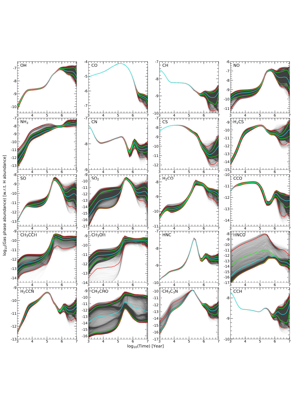
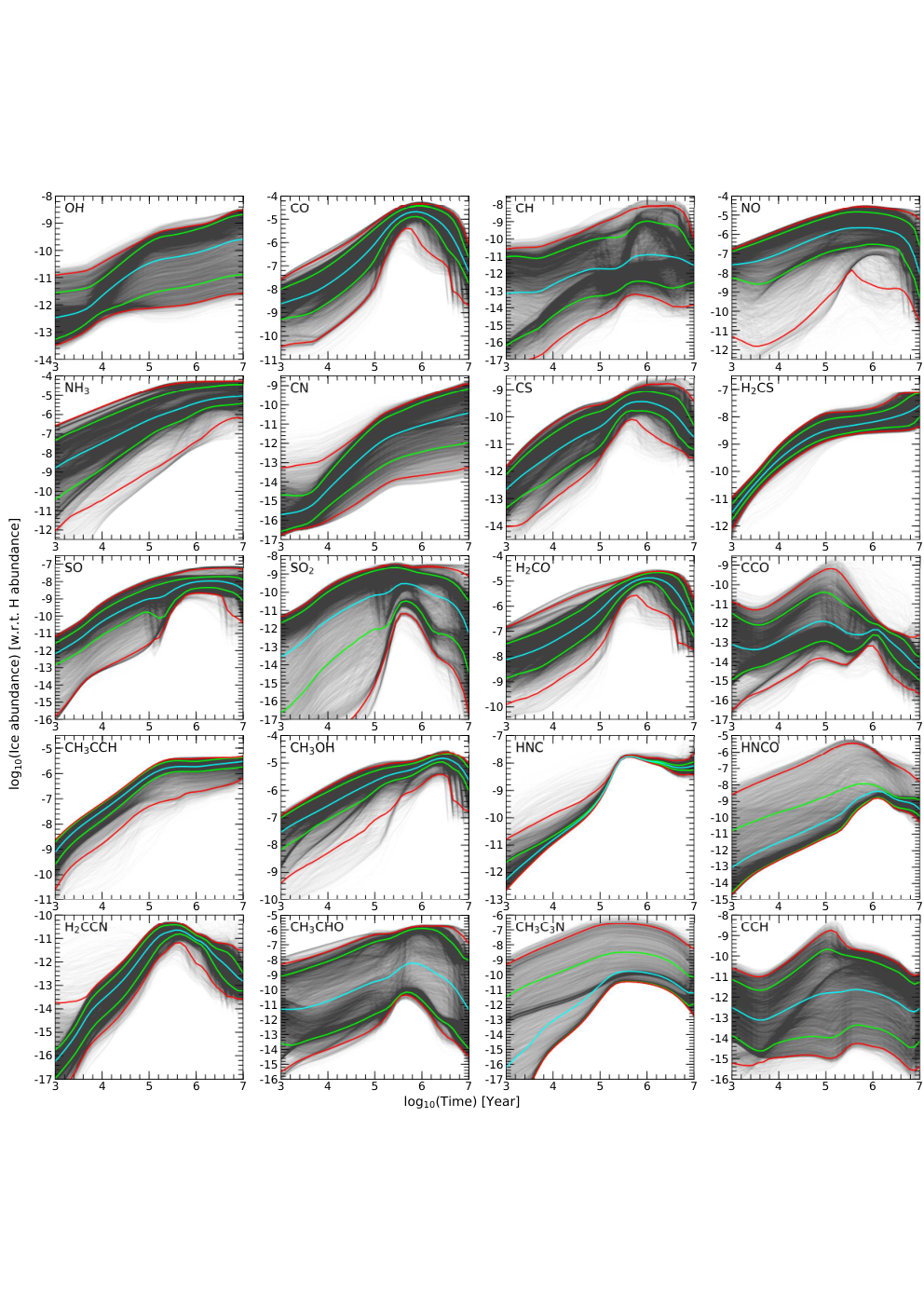
In Fig. 2 we plot the gas-phase abundances of 20 species observed in the dark cloud TMC-1 (CP). We also show the 1 (green lines) and 2 (red lines) deviation and the mean abundance (cyan line) for each species. All the species in Fig. 2 can be divided into two groups. The first group is composed of OH, CO, CH, CN, CS, HNC, and CCH. These species show a negligible variation in their gas-phase abundance until as late as years. After this, the variation in their abundance starts to increase rapidly. These species are essentially those that form in the gas phase, and thus the variations in their abundances in the ice may not correlate with their gas-phase abundances. To verify this, we show in Fig. 3 that these species have indeed large variations in their ice abundances even at early time in the simulation, but the ice abundances are smaller than those of the gas-phase by more than one order. Desorption of these species from the surface therefore does not produce large variation in their gas-phase abundances. At later time, however, when the gas is depleted in heavier elements as a result of freeze-out on dust grains, the formation efficiency of these species in the gas phase is greatly reduced. By this time, the ice abundances become significant, and thus the balance between the freeze-out and the non-thermal desorption processes controls the amount of these species in the gas phase, which causes the observed correlation between the variations in the ice abundances and the gas- hase abundances.
In the second group we collected all other species. These species show significantly large variations in their abundances from very early time in the simulation. This trend indicates that either these species are predominantly formed on the grain surface and the uncertainty in of surface species directly translates into the variation in their abundances, or that the gas-phase abundances of these species strongly depend on other species that predominantly form on the grain surface. One point to note here is that the uncertainty does not always propagate positively with time. This means that we can have a maximum and minimum uncertainty at any time in the simulation. As we clearly see in Fig. 2, SO2, CH3OH and CH3CHO have the maximum uncertainties in abundances at around years and the minimum uncertainties at around years. This behavior strongly depends on whether the species is predominantly formed in the gas phase or on the grain surface, and in the simulation, this may change with time. For example, at the beginning of the simulation, the gas-phase SO2 is predominantly formed through the grain surface reaction
where the prefix J represents the gain surface reaction. By years, however, SO2 is predominantly formed through the gas phase reactions
and
Similarly, at the beginning, CH3OH is only formed on the grain surface through the reactions
and
but around years, it is also formed in the gas phase with significant efficiency thorugh the reactions
and
although it is still formed predominantly on the grain surface. We found a similar trend for other species as well. This is no surprise as the uncertainty in produces the uncertainty in the grain surface reaction rates alone. Therefore we expect a higher uncertainty when a certain species is predominantly formed on the grain surface, a reduced uncertainty when the species is formed significantly in the gas phase, and absolutely no uncertainty when it is solely formed in the gas phase.
3.2 Identification of key species
| Case | Species with constant | Number of simulations |
|---|---|---|
| Case A | Only H | 10000 |
| Case B | H, H2, N, O, CO, and CH3 | 2000 |
| Case C | All species in case B plus | 2000 |
| CH2, HCO, S, and O2 | ||
| Case D | All species in cases A and B | 2000 |
| plus NO, HS, and CH |
One of our objectives here is to identify the key species (if possible) for which a better estimate of would greatly reduce the uncertainties in the computed abundances. For this, we calculated Pearson correlation coefficients () (Penteado et al. 2017, see) between values of 86 key surface species (such as water, CO2 and other species observed in dark clouds) and their abundances in the gas phase and in the ice. Briefly, a Pearson correlation coefficient is a number between -1 and 1 that indicates the extent to which two variables are linearly related. A value of 1 or -1 means a strong correlation and anticorrelation, respectively, while a value of 0 means no correlation at all. Thus in our case, gives a measure of the linear correlation or anticorrelation between values and the ice abundances of selected species.
On the basis of , we divided all species into four groups. In the first group we have species with absolute values of equal to or greater than 0.3 for most of the species. H2 ( 440K, Wakelam et al. 2017), N ( 800K, Tielens & Hagen 1982),O ( 800K, Tielens & Allamandola 1987), CO ( 1150K, OSU database), and CH3 ( 1175K, OSU database) are the species in this group. In the second group we have (CH2 (1050K, OSU database), HCO ( 1600K, OSU database), S ( 1100K, OSU database), and O2 ( 1000K, OSU database) in decreasing order of the number of species that they are correlated or anticorrelated with) species with the absolute value of equal to or greater than 0.3 for a considerable number of the species, but a weak correlation. In the third group we have NO ( 1600K, OSU database), HS ( 1450K, OSU database), and CH ( 925K, OSU database). These species are correlated or anticorrelated with only a few species. In the last group we have all other species. The values of these species show no correlation or anticorrelation with the abundances of other species. Although carbon is the fourth most abundant species (see Table 2), it is to be noted that the diffusion of C atoms does not introduce any noticeable uncertainties in the ice abundances of any species. This is because in our model the (= 4000K) value of the C atom is taken from Ruaud et al. 2015, and Wakelam et al. 2017 also found similar values for the carbon atom. Such a high value of makes diffusion of carbon atoms inefficient.
value gives a good idea about which species to look for giving maximum variation in the abundances of any particular species, but most often, this information alone is not enough to find the reactions that cause the variation in the species abundance. For example, in Fig. 2 we see the large variation in the abundance of HNCO in both the gas phase and on ice, but we find no strong correlation with any surface species (see Fig. 4). The HNCO molecule is predominantly formed on the grain surface through the reaction
The chemical desorption during this reaction is responsible for the HNCO in the gas phase. The OCN on the grains mostly comes from the adsorption of gas-phase OCN, which is correlated to CO, N, O, and CH3 (see Fig. 4). Gas-phase OCN is formed by
while HCO in the gas comes from the hydrogenation of CO on the grains. Thus, based on all these reactions, we can determine how the variation in of CO propagates to HNCO.
Now, we show three cases (cases B, C, and D, see Table 3) with 2000 new simulations in each case and compare it with case A, which we have discussed in the previous section. To recall, in case A we varied for all species except for H. In comparison, in case B we kept constant at 0.4 for all the species in group 1 (H2, N, O, CO, and CH3) in all 2000 simulations and varied for all other species except for H. In case C we kept constant at 0.4 for all the species in the second group (H2, N, O, CO, CH3, CH2, HCO, S, and O2) in all 2000 simulations and varied for all other species except for H. In case D we kept constant at 0.4 for H2, N, O, CO, CH3, CH2, HCO, S, O2, NO, HS, and CH in all 2000 simulations and varied for all other species except for H.
In Fig. 5 we plot the gas-phase abundances within 2 variation for 42 key species. The figure clearly shows the effect of restricting the values of species in the sorted groups and how they affect the gas-phase abundances of other species. By comparing the areas below the gray and green curves, we see that uncertainties in the gas-phase abundances of most of the simple species, OH, CO, CN, N2, NO, NH3, H2O, CO2 etc., and some complex species, CH3O, CH3OH etc., can be reduced to just a very small fraction of the actual uncertainties by just restricting the uncertainties in the mobilities of five key species (H2, N, O, CO, and CH3). Furthermore, the area below the red curve shows that if we can do the same for other four species (CH2, HCO, S, and O2), then the uncertainties in the gas-phase abundances are reduced significantly for almost all the species except for a few, which depend strongly on the mobility of mostly NO in the ice. We therefore further limited the values of NO, HS, and CH and found that there are almost no uncertainties in the gas-phase abundances of any species because the blue curve appears just like a thin line. We did not find a noticeable uncertainty in the ice abundances either, with only a few species as exceptions. We found a few species in the network that strongly depend on the mobility of other species such as CN or C2 . To show this, we plot the ice abundances of CCH and H2CCN in Fig. 6. Even after restricting the values of for all identified species, we have a huge uncertainty in the ice abundance of CCH and a small but visible uncertainty in the ice abundance of H2CCN. Basically, the huge uncertainty in the ice abundance of CCH comes from the uncertainty in of C2 as CCH is formed in the ice through the reaction
and the uncertainty in the ice abundance of H2CCN comes from the uncertainty in of CN through the reaction
The results shown above clearly suggest that the uncertainties (as far as the uncertainty in the chemical network that is due to the mobility of adsorbed species is concerned) in the abundances (both the gas phase and the ice) of most of the species can be very much removed by fixing the value of for 13 species, including H. Some species still are an exception and can be treated on a case basis if needed in the future.
3.3 Effect of the uncertainties in of individual species
In this section we evaluate how the uncertainties in the values of of each of the species H2, N, O, CO, and CH3 individually affect the evolution of the chemical network. For this we ran 51 simulations in which we varied the values of for one of the species H2, N, O, CO, and CH3. Thus we ran five sets of simulations with 51 simulations in each set (one for each species). In the first set of simulations, we varied the value of of CH3 between 0.25 to 0.75 with an increase of 0.1 in each subsequent simulation and kept it constant at 0.4 for all other species. In the following sets of simulations, we repeated this for the other species listed above. In this way, we can determine the effect of the mobility of one single species.
In Fig. 7 we plot the gas-phase abundances of six species (these species show high sensitivity to values of the selected species in case B) at years as a function of of the selected species. In all plots, we see a common trend that there is a certain range of within which any change in the value of results in noticeable changes in the species abundances. In the case of CO, we see that when varies between 0.25 and 0.35, there are rapid changes in the abundances of the plotted species, but for any value of above 0.35, we obtain flat lines. For O we see the same range, but when is between 0.45 and 0.6. For N, this range is between 0.4 to 0.65, and for CH3 this range is between 0.3 and 0.5. H2 seems to be an exception as we see that any change in its value changes the abundance of plotted species. The very strong sensitivity to the H2 diffusion is due to the reaction-diffusion competition included in the model, which strongly increases the surface reactions with H2.
Furthermore, to verify how this range changes at other times in the simulations, we replotted the same plots, but at and in Fig. 8. We find that the sensitivity range of remains very much the same at different times in the simulation, but as expected, the abundances within the range change quite strongly with time. Thus we can conclude that the abundance of any species is sensitive only within a certain range of values of any surface species, and this range remains very much the same throughout the simulation.
Here we also note if the diffusion timescale of a species becomes shorter than the timescale of the monolayer ice formation, then the diffusion of this species would be unimportant. We can define a critical diffusion energy where the two timescales become comparable. In our simulations, at years, ice is formed at a rate of about monolayers per year, which gives a critical diffusion energy of 532K. This means that the chemical composition should not be much influenced by species with diffusion energies higher than 532K. This critical energy becomes slightly higher with time (as the ice formation slows down): 558K and 589 at and years, respectively.
In Sec. 3.1, when we randomly changed of all species, we obtained large uncertainties in the species abundances, and then in Sec. 3.2, we saw that the greater portion of the uncertainties in the species abundances comes from the uncertainties in the values of only a few surface species. To quantify the contribution of H2, N, O, CO, and CH3 to the total uncertainty in the gas-phase abundances of 80 key species, of which about 60 are observed in TMC-1 (CP), we calculated the total variation in the abundances of these species at and years in each of the five sets of simulations discussed above. This variation gives us the uncertainty that is due to the values of for H2, N, O, CO, and CH3 individually. We also calculated the total uncertainties in the gas-phase abundances of these 80 species in all 10000 simulation discussed in Sec. 3.1. We list all these values in Table . In the first column of the table we list all species. In the next subsequent columns we list the uncertainties in the species abundances. Thus the column with the header means that the column contains uncertainties that are due to the value of of surface species X alone, while of other species was constant at 0.4. These values are in log of base 10, thus an uncertainty of 1 means an uncertainty of order one in the calculated abundance. From this table, we can find the source of the uncertainty in the abundance of any species in greater detail. Here it should be noted that the uncertainties from different sources cannot be summed directly to derive the total uncertainty because in the simulations these species are connected through various chemical networks. When we introduce uncertainties in all of them, then some add and some cancel, and some show other possible outcomes. We still found that a simple addition gives a rough but good estimate of the total uncertainty introduced by selected species, however.
3.4 Sensitivity to the surface temperature
To determine how the uncertainty in the abundance of any species varies with the change in surface temperature, we ran case A again, but this time, we ran 2000 simulations with a surface temperature at 8K and another 2000 simulations with a surface temperature at 12K. The surface temperature was kept at 10K in the first case A presented in Sec. 3.1. We found that the species that are predominantly formed in the gas phase do not show any significant change in the total uncertainties with a change in temperature. Only the mean value of the abundance changes. The species predominantly formed on the grain surface, in contrast, showed noticeable changes in the total uncertainty, but these changes are not unidirectional. For example, species such as CH2OH, HCOOH, HNCO, CS, H2S, and CH3CCH show a jump in the total uncertainty at 12K and a reduction in the total uncertainty at 8K. Other species such as CH3O, N2, HNC, NH3, and CH3OH show a completely opposite trend.
4 Best model and comparison with observations
| Model/Observations | H2O | CO | CO2 | CH3OH | NH3 | CH4 | H2CO | OCS |
| Best-fit model | 100 | 10.74 | 44.04 | 10.02 | 1.52 | 11.70 | 6.41 | 0.04 |
| Nautilus (with ) | 100 | 13.76 | 54.77 | 12.56 | 1.10 | 10.10 | 7.63 | 0.02 |
| BG stars | 100 | nd | ||||||
| MYSOs | 100 | |||||||
| LYSOs | 100 |
We used the simple method of parameter fitting to best fit the observed abundances of 58 species, observed in the dark cloud TMC-1 (CP). We used the observed abundances gathered in Agúndez & Wakelam 2013 for cold cores. In our calculations, we did not use those species for which only the upper or the lower limits of the abundance is given. Knowing that most of the uncertainty in the simulated abundance comes from only a few species, we determined the best value of for H2, CH3, and CO to obtain a better agreement with the observed abundances. Of course, this method assumes that most of the error in the model is mainly due to the uncertainty in .
For comparison with observed abundances, we used the method described in Loison et al. 2014. We computed the mean distance of disagreement for each output of the simulation using the formula
| (8) |
where is the calculated abundance of species at time , is the observed abundance for the same species, and is the total number of observed species used in the calculation of . In this method, the model with the lower value of is the best model because a lower value of means a better agreement between the observed abundances and the simulated results.
To calculate the best-fit values of , we used an iterative method. In this method we fixed at 0.4 for all species except for CO. Then we ran 51 simulations in which we varied between 0.25 to 0.75. Then we compared abundances in all 51 simulations with the observed abundances in TMC-1 (CP) and determined which value of gives the best agreement. Next we fixed at this value and repeated the same process for CH3. We then fixed to its best value and repeated this again for CO. We repeated the same process many times until we converged to the best values of and , which did not change any more. Then we introduced the third species H2 and used the same iterative process to determine the best values of , , and . The best-fit values are 0.33, 0.34, and 0.74, corresponding to diffusion energies of 380K, 399K, and 326K for CO, CH3 , and H2 , respectively. Next, we ran a simulation in which we used the bes- fit values for , , and and kept = 0.4 for all other species. For comparison, we also ran one simulation in which we kept = 0.4 for all species.
In our iterative method for calculating the best-fit values, we only used the observed abundances in TMC-1 (CP). This method does not guarantee that if we use observational data of another cloud, we would also obtain the same best values of . Nevertheless, we also calculated for 34 observed molecules for an other cold core, L134N (N). Again, for observational data for L134N, we used the tabulated values in Agúndez & Wakelam 2013.
In Fig. 9 we show the calculated values for both the best-fit and the standard models and for both clouds. The best-fit model improves the agreement with the observed abundances for both clouds. This improvement is of about 10% in log10 scale (0.1dex); this is closer to a 25% improvement in the linear scale. Furthermore, this is an average or overall improvement in agreement with the observational values of 58 and 34 observed species in TMC-1 (CP) and L134N (N), respectively. When we consider only certain species, then the improvement is quite significant. The best-fit model gives a better agreement for 32 out of 58 species in TMC-1 (CP). For these 32 species, the lowest value of is 0.67 for the best-fit model, while it is 0.86 for the standard model, which is an overall improvement of 22% (in log10 scale). For the other 26 species, the lowest value of is 1.04 for the best-fit model, while it is 0.98 for the standard model. This is a negative change of only 6% (in log10 scale) for the best-fit model.
In Table 4 we show the comparison between the best-fit model, the standard Nautilus model (with ), and the ice abundances observed in the envelopes around young stellar objects (LYSOs), massive young stellar objects (MYSOs), and toward the background stars (BG stars) as given in Boogert et al. 2015. For comparison with simulated results, we used the values at best-fit times (2.99 years). It is to be noted that our simulated results are for dark cloud conditions and do not properly represent the conditions in LYSOs, MYSOs, or the regions toward the BG stars. Nevertheless, for a qualitative study it is good to compare different models with observations. Table 4 shows that the two models are not much different in their results: we observe only a slightly better agreement for the new model. However, both CO2 and CH4 are overproduced by the models.
5 Conclusions
We calculated the uncertainties induced in the gas phase and the ice abundances of the species in simulated results due to the uncertainties in the diffusion energy of adsorbed species. We showed that these uncertainties are very large for species that are predominantly formed on the grain surface, such as CH3OH. Species such as CO, OH, or HNC, which are mainly formed in the gas phase, only show an uncertainty after years in simulations. By this time, we have more than 100 monolayers of ice on the grain surface. This large reservoir of species on the grain surface causes the propagation of uncertainties in the gas-phase abundances.
We identified the surface species, the uncertainties in diffusion rates of which result in the larger variations in abundances of most of the species. CO, H2, O, N, and CH3 are the key species for the uncertainties in the abundances, while CH2, HCO, S, and O2 come next, followed by NO, HS, and CH. We also showed that by limiting the uncertainties in the ratio of diffusion to binding energy of these species, we were able to eliminate the uncertainties in the gas-phase abundances of almost all the species.
We calculated the contribution to the uncertainties in the species abundances coming from CO, H2, O, N, and CH3 individually. We found that there is a small range of (the ratio of diffusion energy to binding energy) for all these species within which we obtain variation in the abundances. The size and position of this range varies with species. For O, it is between 0.45 to 0.6. For N, it is 0.4 to 0.65. For CO, it is 0.25 to 0.36. For CH3, it is 0.36 to 0.5. H2 is an exception and affects the surface chemistry within the entire range of we tested in our simulations. We found that this range remains constant throughout the simulation and thus does not depend on time.
We also tested for different grain surface temperatures and found that although a different surface temperature changes the uncertainty pattern for most of the species, it does not follow a unidirectional increase or decrease in the variation in the species abundances. Thus it is not possible to predict if the uncertainty in the abundance of a certain species will increase or decrease with an increase or decrease of the surface temperature.
We calculated the best values of for CO, CH3 , and H2, using an iterative approach, to better explain the observed abundances in dark dense cloud such as TMC-1(CP). We showed that we can improve the overall agreement by 8% (in log10 scale) for 58 species and 22% (in log10 scale) for 32 species observed in TMC-1 (CP) by just fixing the values of CO, CH3 , and H2 at 0.33, 0.34, and 0.74, respectively.
We provided uncertainties in abundances of a number of species due to individual species (H2, N, O, CO, and CH3) and also cumulative uncertainties due to all surface species in a tabulated form. This table provides an idea of how much error one can expect in their modeling of observed abundances in similar cold cores.
It should be noted that these values and other results presented in this work may depend on the physical conditions of the clouds and also on the model parameters. The surface temperature alone can significantly increase or decrease the uncertainties.
In our simulations, we kept the binding energies of all species constant and only varied the diffusion energy depending on values of . The key species we found are not expected to change in a different set of binding energies unless the difference is very large (hundreds of K). The range of calculated for CO, O, N, and CH3 is expected to shift by a few points left or right until the diffusion energy matches the energy we used in our simulation.
Acknowledgements.
This study has received financial support from the French State in the frame of the ”Investments for the future” Programme IdEx Bordeaux, reference ANR-10-IDEX-03-02. The research of VW is funded by an ERC Starting Grant (3DICE, grant agreement 336474) and the CNRS program Physique et Chimie du Milieu Interstellaire (PCMI), co-funded by the Centre National d’Etudes Spatiales (CNES).References
- Agúndez & Wakelam (2013) Agúndez, M. & Wakelam, V. 2013, Chemical Reviews, 113, 8710
- Al-Halabi & van Dishoeck (2007) Al-Halabi, A. & van Dishoeck, E. F. 2007, MNRAS, 382, 1648
- Biham et al. (2001) Biham, O., Furman, I., Pirronello, V., & Vidali, G. 2001, ApJ, 553, 595
- Boogert et al. (2015) Boogert, A. C. A., Gerakines, P. A., & Whittet, D. C. B. 2015, ARA&A, 53, 541
- Chang et al. (2005) Chang, Q., Cuppen, H. M., & Herbst, E. 2005, A&A, 434, 599
- Chang et al. (2007) Chang, Q., Cuppen, H. M., & Herbst, E. 2007, A&A, 469, 973
- Garrod & Pauly (2011) Garrod, R. T. & Pauly, T. 2011, ApJ, 735, 15
- Gould et al. (1963) Gould, R. J., Gold, T., & Salpeter, E. E. 1963, ApJ, 138, 408
- Graedel et al. (1982) Graedel, T. E., Langer, W. D., & Frerking, M. A. 1982, ApJS, 48, 321
- Hasegawa & Herbst (1993) Hasegawa, T. I. & Herbst, E. 1993, MNRAS, 263, 589
- Hasegawa et al. (1992) Hasegawa, T. I., Herbst, E., & Leung, C. M. 1992, ApJS, 82, 167
- Hincelin et al. (2011) Hincelin, U., Wakelam, V., Hersant, F., et al. 2011, A&A, 530, A61
- Hollenbach & Salpeter (1970) Hollenbach, D. & Salpeter, E. E. 1970, J. Chem. Phys., 53, 79
- Jenkins (2009) Jenkins, E. B. 2009, ApJ, 700, 1299
- Karssemeijer & Cuppen (2014) Karssemeijer, L. J. & Cuppen, H. M. 2014, A&A, 569, A107
- Livingston et al. (2002) Livingston, F. E., Smith, J. A., & George, S. M. 2002, The Journal of Physical Chemistry A, 106, 6309
- Loison et al. (2014) Loison, J.-C., Wakelam, V., Hickson, K. M., Bergeat, A., & Mereau, R. 2014, MNRAS, 437, 930
- Mispelaer et al. (2013) Mispelaer, F., Theulé, P., Aouididi, H., et al. 2013, A&A, 555, A13
- Penteado et al. (2017) Penteado, E. M., Walsh, C., & Cuppen, H. M. 2017, ApJ, 844, 71
- Ruaud et al. (2015) Ruaud, M., Loison, J. C., Hickson, K. M., et al. 2015, MNRAS, 447, 4004
- Ruaud et al. (2016) Ruaud, M., Wakelam, V., & Hersant, F. 2016, MNRAS, 459, 3756
- Stecher & Williams (1966) Stecher, T. P. & Williams, D. A. 1966, ApJ, 146, 88
- Tielens & Allamandola (1987) Tielens, A. G. G. M. & Allamandola, L. J. 1987, in Astrophysics and Space Science Library, Vol. 134, Interstellar Processes, ed. D. J. Hollenbach & H. A. Thronson, Jr., 397–469
- Tielens & Hagen (1982) Tielens, A. G. G. M. & Hagen, W. 1982, A&A, 114, 245
- Wakelam & Herbst (2008) Wakelam, V. & Herbst, E. 2008, ApJ, 680, 371
- Wakelam et al. (2015) Wakelam, V., Loison, J.-C., Herbst, E., et al. 2015, ApJS, 217, 20
- Wakelam et al. (2017) Wakelam, V., Loison, J.-C., Mereau, R., & Ruaud, M. 2017, Molecular Astrophysics, 6, 22
- Watanabe et al. (2010) Watanabe, N., Kimura, Y., Kouchi, A., et al. 2010, ApJ, 714, L233
- Watson (1976) Watson, W. D. 1976, Reviews of Modern Physics, 48, 513
- Watson & Salpeter (1972) Watson, W. D. & Salpeter, E. E. 1972, ApJ, 174, 321
- Williams (1971) Williams, D. A. 1971, The Observatory, 91, 225