Spherically symmetric static vacuum solutions in hybrid metric-Palatini gravity

Bogdan D

\check{\mathrm{a}}

nil

\check{\mathrm{a}}

Email: bogdan.danila22@gmail.com Affiliation: Astronomical Observatory, 19 Ciresilor Street, Cluj-Napoca, Romania, Affiliation: Department of Physics, Babes-Bolyai University, Kogalniceanu Street, Cluj-Napoca 400084, Romania, Tiberiu Harko Email: t.harko@ucl.ac.uk Affiliation: Department of Physics, Babes-Bolyai University, Kogalniceanu Street, Cluj-Napoca 400084, Romania, Affiliation: School of Physics, Sun Yat-Sen University, Guangzhou 510275, People’s Republic of China Affiliation: Department of Mathematics, University College London, Gower Street, London WC1E 6BT, United Kingdom, Francisco S. N. Lobo Email: fslobo@fc.ul.pt Affiliation: Instituto de Astrofísica e Ciências do Espaço, Faculdade de Ciências da Universidade de Lisboa, Edifício C8, Campo Grande, P-1749-016 Lisbon, Portugal, Man Kwong Mak Email: mankwongmak@gmail.com Affiliation: Departamento de Física, Facultad de Ciencias Naturales, Universidad de Atacama, Copayapu 485, Copiapó, Chile

August 11, 2026

Abstract

We consider vacuum static spherically symmetric solutions in the hybrid metric-Palatini gravity theory, which is a combination of the metric and Palatini $f(R)$ formalisms unifying local constraints at the Solar System level and the late-time cosmic acceleration. We adopt the scalar-tensor representation of the hybrid metric-Palatini theory, in which the scalar-tensor definition of the potential can be represented as a Clairaut differential equation. Due to their mathematical complexity, it is difficult to find exact solutions of the vacuum field equations, and therefore we adopt a numerical approach in studying the behavior of the metric functions and of the scalar field. After reformulating the field equations in a dimensionless form, and by introducing a suitable independent radial coordinate, the field equations are solved numerically. We detect the formation of a black hole from the presence of Killing horizon for the time-like Killing vector in the metric tensor components. Several models, corresponding to different functional forms of the scalar field potential are considered. The thermodynamic properties of these black hole solutions (horizon temperature, specific heat, entropy and evaporation time due to Hawking luminosity) are also investigated in detail.

pacs

04.50.Kd, 04.40.Dg, 04.20.Cv, 95.30.Sf

I Introduction

The observational discovery of the recent acceleration of the Universe 1n; 2n; 3n; 4n; acc has raised the fundamental theoretical problem if general relativity, in its standard formulation, can fully account for all the observed phenomena at both galactic and extra-galactic scales. The simplest theoretical explanation for the observed cosmological dynamics consists in slightly modifying the Einstein field equations, by adding to it a cosmological constant $\Lambda$ Wein. Together with the assumption of the existence of another mysterious component of the Universe, denoted dark matter dm1; dm2, and assumed to be cold, the Einstein gravitational field equations can give an excellent fit to all observational data, thus leading to the formulation of the standard cosmological paradigm of our present days, called the $\Lambda$ CDM model. However, despite its apparent simplicity and naturalness, the introduction of the cosmological constant raises a number of important questions for which no convincing answers have been provided so far. Thus, the $\Lambda$ CDM model can fit the observational data at a high level of precision, and despite being a very simple theoretical approach, no fundamental theory can explain it. Why is the cosmological constant so small and so fine-tuned? Why did the Universe begin to accelerate so recently? And, after all, why is a cosmological constant necessary at all?

From a theoretical point of view two possible answers to the questions raised by the recent acceleration of the Universe can be formulated. The first, we may call the dark energy approach, assumes that the Universe is filled by a mysterious and unknown component, called dark energy PeRa03; Pa03; 8; Tsu, which is fully responsible for the accelerated expansion of the Universe. The cosmological constant may correspond to a particular phase of the dynamical dark energy (ground state of a potential, let’s say), and the recent de Sitter phase may prove to be just an attractor of the dynamical system describing the cosmological evolution. A second approach, the dark gravity approach, assumes the alternative possibility that at large scales the gravitational force may have a behavior different from that suggested by standard general relativity. In the general relativistic description of gravity, the starting point is the Hilbert-Einstein action, which can be written down as $S=\int{\left(R/2\kappa^{2}+L_{m}\right)\sqrt{-g}\;d^{4}x}$ , where $R$ is the Ricci scalar, $\kappa$ is the gravitational coupling constant, and $L_{m}$ is the matter Lagrangian, respectively. Hence, in dark gravity theories for a full understanding of the gravitational interaction a generalization of the Hilbert-Einstein action is necessary.

There are two possibilities to construct dark gravity theories. The first is based on the modification of the geometric part of the Hilbert-Einstein Lagrangian only. An example of such an approach is the $f(R)$ gravity theory, introduced in Bu; Ba, and in which the geometric part of the action is generalized so that it becomes an arbitrary function $f(R)$ of the Ricci scalar. Hence, in $f(R)$ gravity the total Hilbert-Einstein action can be written as $S=\int{\left[f(R)/2\kappa^{2}+L_{m}\right]\sqrt{-g}\;d^{4}x}$ . The recent cosmological observations can be satisfactorily explained in the $f(R)$ theory, and a solution of the dark matter problem, interpreted as a geometric effect in the framework of the theory, can also be obtained dm3. In a more general approach one modifies both the geometric and the matter terms in the Hilbert-Einstein action, thus allowing a coupling between matter and geometry Bert; Harkof. For reviews and in depth discussions of $f(R)$ and other modified gravity theories see r1; r2; r3; r4; rn; r5; r6; r7; r8; r9.

Einstein’s general theory of relativity can be obtained by starting from two different theoretical approaches, called the metric and the Palatini formalisms Olmo, respectively. When applied to the Hilbert-Einstein action, these two approaches lead to the same gravitational field equations, with the Palatini formalism also providing the explicit expression of the symmetric connection in terms of the derivatives of the metric tensor. However, in $f(R)$ gravity, as well as in other modified theories of gravity, this does not happen anymore, and it turns out that the gravitational field equations obtained using the metric approach are generally different from those obtained by using the Palatini variation Olmo. An important difference is related to the order of the field equations, with the metric formulation usually leading to higher-order derivative field equations, while in the Palatini approach the derived field equations are always second order partial differential equations. On the other hand, in the Palatini variational formulation a number of new algebraic relations appear, which involve the matter fields and the affine connection, such that the connection can be determined from a set of equations which couples it to the metric and to the matter fields.

Based on a hybrid combination of the metric and Palatini mathematical formalisms, an extension of the $f(R)$ gravity theory was proposed in h1. In this approach the (purely metric) Hilbert-Einstein action is generalized by adding to it (metric-affine) correction terms obtained in the spirit of the Palatini approach. Simple extensions of standard general relativity with interesting properties can be constructed using both metric and Palatini $f(R)$ theories. However, in each of these theories a number of different pathological behaviors appear. Hence, by building a bridge that relates these two apparently different approaches we may find a possibility of removing their individual failures.

A hybrid combination of the metric and Palatini formalisms was used in h1; h2 to construct a new type of gravitational Lagrangian. This gravitational theory is called hybrid metric-Palatini gravity (HMPG). From a theoretical point of view the main result of this approach is that viable gravity theories including elements of both formalisms can be obtained. Moreover, in this class of theories it is possible to generate long-range forces that do not contradict the classical local Solar System tests of gravity. The analysis of the field equations and the construction of solutions is greatly simplified with the use of the scalar-tensor representation of the hybrid metric-Palatini theories. A simple example of such a hybrid metric-Palatini theory can be constructed by adopting for the gravitational Lagrangian the expression $R+f(\mathcal{R})$ , where $\mathcal{R}$ is the Palatini scalar curvature. Such a gravitational action maintains all the well-confirmed results of general relativity, which are included in the Hilbert-Einstein part of the action $R$ , and which describes with a high precision gravitational phenomena at the scale of the Solar System and of compact objects. On the other hand the metric-affine component $f(\mathcal{R})$ generates novel physical characteristics that may explain the recent cosmological observations of the accelerating Universe. In Ko1; Ko2 a similar formalism that interpolate between the metric and Palatini regimes was proposed for the study of $f(R)$ type theories. This approach is called the C-theory. In B1a a generalization of HMPG was introduced.

The study of the cosmological and astrophysical implications of HMPG has attracted a lot of attention recently. The properties of the Einstein static Universe in HMPG were studied in B. Cosmological solutions obtained with the help of the scalar-tensor representation of the theory were presented in c1, were their cosmological applications were also investigated. The cosmological field equations were formulated as a dynamical system, and, by adopting some specific functional forms of the effective scalar field potential, several classes of cosmological solutions were obtained. The dynamical system approach was generalised in c5, where new accelerating solutions that can be attractors in the phase space were found. In c4 the evolution of the linear perturbations in HMPG was considered. The full set of linearized evolution equations for the perturbed physical and geometrical quantities were obtained, and it was shown that important deviations from the $\Lambda$ CDM model occur in the far past, with ratio between the Newtonian potentials $\Phi$ and $\Psi$ presenting an oscillatory signature. Cosmological models were studied in c6. By using a combination of baryonic acoustic oscillations, supernovae and cosmic microwave background data, the free parameters of the models can be constrained. The analysis was further generalized using a specific HMPG model, given by $f(R)\propto R^{2}$ new1, and the results were compared with the local constraints.

In the scalar-tensor representation of the HMPG theory, new cosmological solutions were obtained in new2 by either making an ansatz on the scale factor or on the effective potential. The efficiency of screening mechanisms in the hybrid metric-Palatini gravity was investigated in new3. Bounds on the model were obtained using data from Solar System experiments, and they can contribute to fix the range of viable hybrid gravity models. Gödel-type solutions, in which the matter source is a combination of a scalar with an electromagnetic fields, plus a perfect fluid were obtained in the framework of HMPG theory in new4. The existence of Gödel-type solutions indicates that HMPG does not solve the causal anomaly in the form of closed timelike curves that appears in general relativity.

HMPG also opens some new perspectives for the study of dark matter. The virial theorem for galaxy clusters in HMPG was derived in c2. It turns out that the total virial mass of the cluster is proportional to the effective mass associated to the mass of the effective scalar field. Therefore, the virial mass discrepancy in clusters of galaxies can be explained via the geometric terms appearing in the generalized virial theorem. The HMPG dark matter model also predicts that the effects of the effective mass associated to the scalar field extend far beyond the virial radii of the clusters of galaxies. HMPG also allows for an explanation of the behavior of the rotational velocities of test particles gravitating around galaxies c3. In the equivalent scalar-tensor description the rotational velocity can be obtained explicitly as a function of the scalar field. Hence all the geometric and physical quantities, as well as the coupling constant in HMPG can be expressed as functions of measurable or observable parameters, such as, for example, the stellar dispersion velocity, the Doppler frequency shifts, the baryonic mass of the galaxy, and the tangential velocity, respectively.

The HMPG theory has also been explored in a plethora of other topics. For instance, the problem of the well-posedness and the well-formulation of the Cauchy problem was discussed in P. Wormhole solutions in HMPG have also been found in Lobo, where it was shown that these exotic geometries are supported by the higher order terms. Specific wormhole solutions in a generalized HMPG theory were also found new5. In these solutions the matter field obeys the null energy condition (NEC) everywhere, including the throat and up to infinity, so that there is no need for exotic matter. In the context of compact objects, the internal structure and the physical properties of specific classes of neutron, quark and Bose-Einstein Condensate stars in HMPG were considered in B1. For reviews of HMPG theories, we refer the reader to rev and book, respectively.

Since Karl Schwarzschild obtained the first exact solution of the general relativistic field equations in vacuum Sch1, the search for black hole type solutions describing the gravitational field outside massive gravitating bodies proved to be of fundamental importance for the theoretical understanding and observational testing of gravitational theories (see 0 for a review of the exact solutions of the Einstein field equations). Black hole solutions allow testing the properties of the gravitational force by using the electromagnetic emissivity properties of thin disks that form around compact objects A1; A2; A3; A4; A5; A6; A7; A8; A9; A10; A11; A12; A13; A14; A15. For a review of the possibilities of testing black hole candidates by using electromagnetic radiation see RB.

Many black hole type solutions have been obtained in different modified theories of gravity, such as in brane world models Br0; Br1; Br2; Br3, Eddington-inspired Born-Infeld Bh1, higher derivative gravitational theory with a pair of complex conjugate ghosts Bh2, de Rham-Gabadadze-Tolley (dRGT) theory Bh3, Gauss-Bonnet massive gravity coupled to Maxwell and Yang-Mills fields in five dimensions Bh4, in the framework of the Poincaré gauge field theory with dynamical massless torsion Bh5, Rastall theory Bh8, second-order generalized Proca theories with derivative vector-field interactions coupled to gravity Bh10, mimetic Born-Infeld gravity Bh11, a class of vector-tensor theories of modified gravity Bh12, and dilatonic dyon-like black hole solutions in a model with two Abelian gauge fields were also found Bh6. Black hole solutions that can accommodate both a nonsingular horizon and Yukawa asymptotics have been considered in Bh9. In Bh7 it was shown that a large number of static, spherically symmetric metrics, which are regular at the origin, asymptotically flat, and have both an event and a Cauchy horizon for a certain range of the parameters can be interpreted as exact solutions of the Einstein equations coupled to ordinary linear electromagnetism, that is, as sources of the Reissner-Nordström spacetimes.

In fact, the literature is extremely extensive, and we refer the reader to a solution-generating technique that maps a static charged solution of the Einstein-Maxwell theory in four (or five) dimensions to a five-dimensional solution of the Einstein-Maxwell-Dilaton theory Bh13. Black hole solutions in Gauss-Bonnet-massive gravity in the presence of power-Maxwell field were studied in Bh14; Bh14a; Bh14b; Bh14c. In Bh15 it was shown that black-hole solutions appear as a generic feature of the general Einstein-scalar-Gauss-Bonnet theory with a coupling function $f(\phi)$ . The existing no-hair theorems are easily evaded for this model, and a large number of regular black-hole solutions with scalar hair can be obtained. The properties of black holes in static and spherically symmetric backgrounds in U(1) gauge-invariant scalar-vector-tensor theories with second-order equations of motion were studied in Bh16. Exact asymptotically anti-de Sitter black hole solutions and asymptotically Lifshitz black hole solutions with dynamical exponents $z=0$ and $z=4$ of four-dimensional conformal gravity coupled with a self-interacting conformally invariant scalar field were obtained in Bh17. The vacuum solutions around a spherically symmetric and static object in the Starobinsky model were studied with a perturbative approach in Bh18. Dilatonic black holes in the presence of (non)linear electrodynamics have been studied in Bh19a; Bh19b, respectively.

It is the main goal of the present paper to investigate the possibility of the existence of spherically symmetric static vacuum solutions in the HMPG theory. In order to fulfil this goal, we adopt the scalar-tensor representation of the theory, in which the scalar-tensor definition of the potential can be represented as a Clairaut differential equation. Even in the scalar-tensor representation, resembling the Brans-Dicke theory, the field equations show a high degree of mathematical complexity. Hence it turns out that it is extremely difficult to find exact solutions of the vacuum gravitational field equations, and therefore for the study of the behavior of the metric functions and of the scalar field one must adopt numerical approaches.

The present paper is organized as follows. We briefly present the theoretical foundations and the field equations of HMPG in Section II. The field equations in spherical symmetry for the vacuum case are written down in Section III, where their dimensionless formulation is introduced. Some general properties of the field equations are also discussed. The field equations are solved numerically in Section IV for two particular choices of the scalar field potential, corresponding to a vanishing potential, and a Higgs-type potential, respectively. In each case, the behavior of the metric tensor coefficients and of the effective mass of the scalar field is considered in detail. The thermodynamic properties of the HMPG black holes are investigated in Section V, where the black hole temperature, specific heat, entropy, luminosity and life time are discussed. We discuss and conclude our results in Section VI. In Appendix A we present the details of the transformations of the field equations to a dimensionless form.

II Field equations in HMPG

In the present Section we briefly review the action and the field equations of HMPG. Its scalar-tensor formulation is presented, and the post-Newtonian parameters of the theory are also discussed.

II.1 Action and gravitational field equations

The action for HMPG can be constructed as h1

S=\frac{1}{2\kappa^{2}}\int d^{4}x\sqrt{-g}\left[R+f(\mathcal{R})\right]+S_{m},

(1)

where we have denoted $\kappa^{2}\equiv 8\pi G_{0}/c^{4}$ , while $c$ and $G_{0}$ are the standard speed of light and gravitational constant, respectively; $S_{m}$ is the matter action, defined as $S_{m}=\int d^{4}x\sqrt{-g}\,\mathcal{L}_{m}$ , where $\mathcal{L}_{m}$ is the matter Lagrangean; $R$ is the metric Hilbert-Einstein term, and $\mathcal{R}\equiv g^{\mu\nu}\mathcal{R}_{\mu\nu}$ is the Palatini curvature. The tensor and $\mathcal{R}_{\mu\nu}$ is defined by using an independent connection $\hat{\Gamma}^{\alpha}_{\mu\nu}$ according to

\mathcal{R}_{\mu\nu}\equiv\hat{\Gamma}^{\alpha}_{\mu\nu,\alpha}-\hat{\Gamma}^{\alpha}_{\mu\alpha,\nu}+\hat{\Gamma}^{\alpha}_{\alpha\lambda}\hat{\Gamma}^{\lambda}_{\mu\nu}-\hat{\Gamma}^{\alpha}_{\mu\lambda}\hat{\Gamma}^{\lambda}_{\alpha\nu}\,.

(2)

In the following, the matter energy-momentum tensor $T_{\mu\nu}$ is defined as

T_{\mu\nu}\equiv-\left(\frac{2}{\sqrt{-g}}\right)\frac{\delta(\sqrt{-g}\mathcal{L}_{m})}{\delta g^{\mu\nu}}.

(3)

After varying the action (1) with respect to the metric, we obtain the gravitational field equations of HMPG as

G_{\mu\nu}+F(\mathcal{R})\mathcal{R}_{\mu\nu}-\frac{1}{2}f(\mathcal{R})g_{\mu\nu}=\kappa^{2}T_{\mu\nu},

(4)

where we have denoted $F(\mathcal{R})\equiv df(\mathcal{R})/d\mathcal{R}$ . After varying the action with respect to the independent connection one can easily show that the independent connection is compatible with the metric $F(\mathcal{R})g_{\mu\nu}$ , conformal to $g_{\mu\nu}$ , with the conformal factor given by $F(\mathcal{R})$ . Hence we can obtain the field equations in the equivalent form

	$\displaystyle\mathcal{R}_{\mu\nu}$	$\displaystyle=$	$\displaystyle R_{\mu\nu}+\frac{3}{2}\frac{1}{F^{2}(\mathcal{R})}F(\mathcal{R})_{,\mu}F(\mathcal{R})_{,\nu}$		(5)
			$\displaystyle-\frac{1}{F(\mathcal{R})}\nabla_{\mu}F(\mathcal{R})_{,\nu}-\frac{1}{2}\frac{1}{F(\mathcal{R})}g_{\mu\nu}\Box F(\mathcal{R}).$		(5)

By taking the trace of the field equations (4) we obtain $\mathcal{R}$ in terms of the trace $T$ of the matter energy-momentum tensor as

F(\mathcal{R})\mathcal{R}-2f(\mathcal{R})-R=\kappa^{2}T.

(6)

II.2 Scalar-tensor formulation

By introducing an auxiliary field $E$ , the hybrid metric-Palatini action (1) can be reformulated in the equivalent form of a scalar-tensor theory, having the following action

S=\frac{1}{2\kappa^{2}}\int\mathrm{d}^{4}x\sqrt{-g}[R+f(E)+f^{\prime}(E)(\mathcal{R}-E)],

(7)

(for more technical details, we refer the reader to h1).

As one can easily see, for $E=\mathcal{R}$ , the action given by Eq. (7) reduces to the action (1). Hence, it turns out that if $f^{\prime\prime}(\mathcal{R})\neq 0$ , the field $E$ is dynamically equivalent to the Palatini scalar $\mathcal{R}$ . By introducing the definitions

\phi\equiv f^{\prime}(E),\qquad V(\phi)=Ef^{\prime}(E)-f(E),

(8)

the action takes the form

S=\frac{1}{2\kappa^{2}}\int d^{4}x\sqrt{-g}\left[R+\phi\mathcal{R}-V(\phi)\right]+S_{m}.

(9)

If we vary this action with respect to the metric, the scalar $\phi$ and the connection, respectively, we obtain the following field equations

$\displaystyle R_{\mu\nu}+\phi\mathcal{R}_{\mu\nu}-\frac{1}{2}\left(R+\phi\mathcal{R}-V\right)g_{\mu\nu}$	$\displaystyle=$	$\displaystyle\kappa^{2}T_{\mu\nu},$	(10)
$\displaystyle\mathcal{R}-V_{\phi}$	$\displaystyle=$	$\displaystyle 0\,,$	(11)
$\displaystyle\hat{\nabla}_{\alpha}\left(\sqrt{-g}\phi g^{\mu\nu}\right)$	$\displaystyle=$	$\displaystyle 0,\$	(12)

respectively.

It is interesting to mention that Eq. (8) is a Clairaut differential equation Claraut, that is, it has the form

Ef^{\prime}(E)-f(E)=V\left(f^{\prime}\left(E\right)\right)\,.

(13)

This equation has a linear general solution given by

f(E)=h\,E-V(h)\,,

(14)

where $h$ is a constant, or, equivalently,

f\left(\mathcal{R}\right)=h\,\mathcal{R}-V(h),

(15)

and a singular solution, which can be found from the differential equation

\frac{\partial V\left(f^{\prime}\left(E\right)\right)}{\partial f^{\prime}}-E=0\,.

(16)

Hence in our mathematical formalism for the nonsingular solution of the Clairaut equtation the function $f\left(\mathcal{R}\right)$ is a linear function of the Palatini curvature. In this case for the vacuum state with $T=0$ the trace equation (6) becomes

-h\mathcal{R}-R+2V(h)=0.

(17)

With the use of the non-singular solution (14) we can express the potential $V(\phi)$ of the effective scalar field as

V(\phi)=\left(\phi-h\right)E+V(h),

(18)

giving

E=\mathcal{R}=\frac{V(\phi)-V(h)}{\phi-h}.

(19)

It is interesting to note that when $V(h)>>\left(\phi-h\right)E$ , the scalar field generates an effective cosmological constant, whose numerical value is determined by the functional form of the potential estimated for a constant value of the scalar field.

For a zero scalar field potential, $V\left(\phi\right)\equiv 0$ , from Eq. (19) it follows that $\mathcal{R}=0$ , also giving $R=0$ .

For a potential of the form $V(\phi)=-\left(\mu^{2}/2\right)\phi^{2}+\left(\zeta/4\right)\phi^{4}$ , we obtain

\mathcal{R}=\frac{-\mu^{2}\left(\phi^{2}-h^{2}\right)/2+\zeta\left(\phi^{4}-h^{4}\right)/4}{\phi-h},

(20)

	$\displaystyle R$	$\displaystyle=$	$\displaystyle-h\frac{-\mu^{2}\left(\phi^{2}-h^{2}\right)/2+\zeta\left(\phi^{4}-h^{4}\right)/4}{\phi-h}$		(21)
			$\displaystyle-\mu^{2}h^{2}+\frac{\zeta}{2}h^{4},$		(21)

	$\displaystyle f\left(\mathcal{R}\right)$	$\displaystyle=$	$\displaystyle h\frac{-\mu^{2}\left(\phi^{2}-h^{2}\right)/2+\zeta\left(\phi^{4}-h^{4}\right)/4}{\phi-h}$		(22)
			$\displaystyle+\frac{\mu^{2}}{2}h^{2}-\frac{\zeta}{4}h^{4}.$		(22)

Once the variation of $\phi$ is known from the solution of the gravitational field equations, the Palatini scalar curvature, the metric Hilbert scalar curvature as well as the function $f\left(\mathcal{R}\right)$ can be reconstructed directly, with the trace equation (6) giving the metric Hilbert curvature, while the functional form of $f\left(\mathcal{R}\right)$ follows directly from Eq. (14).

On the other hand, the solution of Eq. (12) shows that the independent connection is the Levi-Civita connection of the metric $h_{\mu\nu}=\phi g_{\mu\nu}$ . Thus, HPMG is a bi-metric theory, with $\mathcal{R}_{\mu\nu}$ and $R_{\mu\nu}$ related by

\mathcal{R}_{\mu\nu}=R_{\mu\nu}+\frac{3}{2\phi^{2}}\partial_{\mu}\phi\partial_{\nu}\phi-\frac{1}{\phi}\left(\nabla_{\mu}\nabla_{\nu}\phi+\frac{1}{2}g_{\mu\nu}\Box\phi\right).

(23)

Therefore the two Ricci scalars are related as

\mathcal{R}=R+\frac{3}{2\phi^{2}}\partial_{\mu}\phi\partial^{\mu}\phi-\frac{3}{\phi}\Box\phi.

(24)

With the help of this relation we eliminate now in action (9) the independent connection. Thus we obtain the following scalar-tensor representation of HMPG h1,

S=S_{g}\left(g,\phi\right)+S_{m},

(25)

where $S_{g}\left(g,\phi\right)$ is given by

	$\displaystyle S_{g}\left(g,\phi\right)$	$\displaystyle=$	$\displaystyle\frac{1}{2\kappa^{2}}\int d^{4}x\sqrt{-g}\Big[(1+\phi)R$		(26)
			$\displaystyle+\frac{3}{2\phi}\partial_{\mu}\phi\partial^{\mu}\phi-V(\phi)\Big].$		(26)

Despite some superficial analogies, this action essentially differs in their couplings of the scalar to the curvature from the $w=-3/2$ Brans-Dicke theory action. However, it belongs to the class of general Bergmann-Wagoner-Nordtvedt scalar-tensory theories N1; N2; N3, whose action for the vacuum state is given by

S=\frac{1}{2\kappa^{2}}\int{\left[f\left(\phi\right)R+g\left(\phi\right)\partial_{\mu}\phi\partial^{\mu}\phi+\lambda\left(\phi\right)\right]\sqrt{-g}d^{4}x},

(27)

where $f(\phi)$ , $g(\phi)$ and $\lambda(\phi)$ are arbitrary functions of the scalar field $\phi$ . A comparison with the action (26) of the HMPG theory in the scalar-tensor representation shows that its action is indedd of Bergmann-Wagoner-Nordtvedt type, with $f(\phi)=1+\phi$ , $g(\phi)=3/2\phi$ , and $\lambda(\phi)=-V(\phi)$ , respectively. An important property of the Bergmann-Wagoner-Nordtvedt theories is that by means of the transformations N2

\bar{g}_{\mu\nu}=f(\phi)g_{\mu\nu},\frac{d\phi}{d\bar{\phi}}=f(\phi)\left[f(\phi)g(\phi)-\frac{3}{2}\left(\frac{df(\phi)}{d\phi}\right)^{2}\right],

(28)

the action (27) can be transformed to the form

S=\frac{1}{2\kappa^{2}}\int{\left[\bar{R}-n\bar{g}^{\mu\nu}\partial_{\mu}\bar{\phi}\partial_{\nu}\bar{\phi}+2\lambda\left(\bar{\phi}\right)\right]\sqrt{-\bar{g}}d^{4}x},

(29)

where $n=\pm 1$ . A crucial mathematical requirement for transformations (28) to be valid is that they must be nonsingular for the considered range of the scalar field variable.

Let’s apply now the transformations (28) to the action (26) of the HMPG theory. We introduce first the conformal transformation of the metric $\bar{g}_{\mu\nu}=\left(1+\phi\right)g_{\mu\nu}$ , which transforms the action (26) to the Einstein frame form

S=\frac{1}{2\kappa^{2}}\int{\left[\bar{R}+\frac{3}{2\phi}\frac{\bar{g}^{\mu\nu}\partial_{\mu}\phi\partial_{\nu}\phi}{\left(1+\phi\right)^{2}}-\frac{V(\phi)}{\left(1+\phi\right)^{2}}\right]\sqrt{-\bar{g}}d^{4}x}.

(30)

Next, we introduce the scalar field transformation

\phi=\tan^{2}\left(\sqrt{\frac{3}{8}}\;\bar{\phi}\right),

(31)

which follows from the second equation in (28). This transformation will transform the HMPG vacuum theory into a canonical scalar field theory with a very specific potential. However, the transformation $\phi\rightarrow\bar{\phi}$ given by Eq. (31) is singular, with $\phi=0$ for $\bar{\phi}=\sqrt{8/3}k\pi$ , $k=0,1,2,3...$ , and $\phi\rightarrow\infty$ for $\bar{\phi}\rightarrow\sqrt{8/3}\left[\left(-1\right)^{k}\pi/2+2k\pi\right]$ , $k=0,1,2,...$ . Hence, even that one could find the solution of the vacuum field equations of the HMPG theory in the canonical scalar field representation in the Einstein frame, there is no guarantee that the obtained solution would generate mathematically consistent and well behaved solutions of the field equations in the Jordan frame, in which the HMPG theory is naturally formulated.

For the sake of comparison we will also briefly present the case of the standard Brans-Dicke theory Dicke1; Dicke2, with the vacuum gravitational action given by

S=\frac{1}{2\kappa^{2}}\int{\left(\phi R-\frac{\omega}{\phi}g^{\mu\nu}\partial_{\mu}\phi\partial_{\nu}\phi\right)\sqrt{-g}d^{4}x},

(32)

which with the help of the transformations

\bar{g}_{\mu\nu}=\phi g_{\mu\nu},\phi=e^{\bar{\phi}},

(33)

can be transformed into the canonical form

S=\frac{1}{2\kappa^{2}}\int{\left[\bar{R}-\left(\omega+\frac{3}{2}\right)\bar{g}^{\mu\nu}\partial_{\mu}\bar{\phi}\partial_{\nu}\bar{\phi}\right]\sqrt{-\bar{g}}d^{4}x}.

(34)

As one can easily see from Eq. (33), the transformation law $\phi\rightarrow\bar{\phi}$ of the scalar field in the Brans-Dicke theory is nonsingular, except for $\bar{\phi}\rightarrow\pm\infty$ . This makes the scalar field transformation mathematical properties in standard Brans-Dicke theory different as compared to the transformation (31) of the scalar field in HMPG theory.

By substituting Eq. (11) and Eq. (23) in Eq. (10), we can write the metric field equation as an effective Einstein field equation given by

G_{\mu\nu}=\kappa^{2}T^{\mathrm{eff}}_{\mu\nu},

(35)

where the effective energy-momentum tensor is defined according to

	$\displaystyle T^{\mathrm{eff}}_{\mu\nu}$	$\displaystyle=$	$\displaystyle\frac{1}{1+\phi}\Bigg\{T_{\mu\nu}-\frac{1}{\kappa^{2}}\Bigg[\frac{1}{2}g_{\mu\nu}\left(V+2\Box\phi\right)+\nabla_{\mu}\nabla_{\nu}\phi$		(36)
			$\displaystyle-\frac{3}{2\phi}\partial_{\mu}\phi\;\partial_{\nu}\phi+\frac{3}{4\phi}g_{\mu\nu}(\partial\phi)^{2}\Bigg]\ \Bigg\}.$		(36)

The scalar field is governed by an effective Klein-Gordon type second-order evolution equation, given by

-\Box\phi+\frac{1}{2\phi}\partial_{\mu}\phi\partial^{\mu}\phi+\frac{\phi[2V-(1+\phi)V_{\phi}]}{3}=\frac{\phi\kappa^{2}}{3}T\,,

(37)

(we refer the reader to h1 for more details on the derivation of this equation). The Klein-Gordon evolution equation indicates that, unlike in the Brans-Dicke ( $w=-3/2$ ) case, in the present theory the scalar field is dynamical. Therefore, the theory does not experience the microscopic instabilities that emerge in Palatini models with infrared corrections Olmo. As for the matter energy-momentum tensor, it turns out that it is independently conserved, and hence it satisfies the standard condition $\nabla_{\mu}T^{\mu}_{\nu}=0$ .

II.3 The post-Newtonian parameters

The post-Newtonian parameters of gravitational theories are important indicators that help us to determine the viability of the theory by using local gravitational tests. In this respect we consider the post-Newtonian analysis of HMPG, where we perturb Eqs. (36) and (37) in a Minkowskian background. We introduce first a quasi-Minkowskian coordinate system, in which $g_{\mu\nu}\approx\eta_{\mu\nu}+h_{\mu\nu}$ , with $|h_{\mu\nu}|\ll 1$ , and we take $\phi=\phi_{0}+\varphi(x)$ , where $\phi_{0}$ denotes the asymptotic value of the field far away from the gravitating sources. Hence for this class of theories we can obtain the standard post-Newtonian metric up to second order, together with the following expressions of the relevant astrophysical parameters (we refer the reader to rev for details)

$\displaystyle G_{\mathrm{eff}}$	$\displaystyle\equiv$	$\displaystyle\frac{\kappa^{2}}{8\pi(1+\phi_{0})}\left(1+\frac{\phi_{0}}{3}e^{-m_{\varphi}r}\right),$	(38)
$\displaystyle\gamma$	$\displaystyle\equiv$	$\displaystyle\frac{\left[1+\phi_{0}\exp\left(-m_{\varphi}r\right)/3\right]}{\left[1-\phi_{0}\exp\left(-m_{\varphi}r\right)/3\right]},$	(39)
$\displaystyle m_{\varphi}^{2}$	$\displaystyle\equiv$	$\displaystyle\frac{1}{3}\left[2V-V_{\phi}-\phi(1+\phi)V_{\phi\phi}\right]\big\|_{\phi=\phi_{0}}\,.$	(40)

In HMPG there are two possibilities to obtain the value $\gamma\approx 1$ of the PPN parameter $\gamma$ . The first one is identical to the one used in the $f(R)$ -type theories, and requires the existence of a very massive scalar field rn. The second possibility consists in imposing a very small background scalar field $\phi_{0}\ll 1$ , so that regardless of the magnitude of $m_{\varphi}$ , the Yukawa-type corrections are very small. This latter case leaves the local gravity tests unaffected, but it allows for the existence of a long-range scalar field that can modify the cosmological dynamics of the Universe.

III Spherically symmetric vacuum field equations in HMPG

III.1 Metric and field equations

In the following, we assume that the geometry outside gravitating objects can be represented by the following line element in curvature coordinates,

ds^{2}=-e^{\nu(r)}c^{2}dt^{2}+e^{\lambda(r)}dr^{2}+r^{2}\left(d\theta^{2}+\sin^{2}\theta d\varphi^{2}\right),

(41)

representing a static and spherically symmetric space-time. The metric functions $\nu(r)$ and $\lambda(r)$ are functions of the radial coordinate $r$ only, with the range $0\leq r<\infty$ . At least theoretically, in the framework of HMPG we can construct asymptotically flat spacetimes, in which $\nu(r)\rightarrow 0$ and $\lambda(r)\rightarrow 0$ as $r\rightarrow\infty$ . In the following, our main goal is to investigate vacuum solutions of the HMPG theory, for which all the components of the energy-momentum tensor vanish identically, $T_{\mu\nu}\equiv 0$ .

Using the metric (41), the effective Einstein field equation (36) provides the following set of vacuum gravitational field equations

	$\displaystyle\frac{1}{r^{2}}\left[1-e^{-\lambda}\left(1-r\lambda^{\prime}\right)\right](1+\phi)-e^{-\lambda}\left(\phi^{\prime\prime}-\frac{3\phi^{\prime 2}}{4\phi}\right)$
	$\displaystyle+\frac{\phi^{\prime}}{2r}e^{-\lambda}\left(r\lambda^{\prime}-4\right)-\frac{V(\phi)}{2}=0,$		(42)

	$\displaystyle\left[\frac{1}{r^{2}}(e^{-\lambda}-1)+\frac{\nu^{\prime}}{r}e^{-\lambda}\right](1+\phi)$
	$\displaystyle+\phi^{\prime}\left(\frac{\nu^{\prime}}{2}+\frac{2}{r}+\frac{3\phi^{\prime}}{4\phi}\right)e^{-\lambda}+\frac{V(\phi)}{2}=0\,,$		(43)

	$\displaystyle\Bigg[\left(\frac{\nu^{\prime\prime}}{2}+\left(\frac{\nu^{\prime}}{2}\right)^{2}+\frac{\nu^{\prime}}{2r}\right)e^{-\lambda}-\frac{1}{2}\frac{\lambda^{\prime}e^{-\lambda}}{r}\left(1+r\frac{\nu^{\prime}}{2}\right)\Bigg]$
	$\displaystyle\times(1+\phi)+\left[\phi^{\prime\prime}+\frac{\phi^{\prime}\nu^{\prime}}{2}+\frac{3\phi^{\prime 2}}{4\phi}\right]e^{-\lambda}$
	$\displaystyle+\frac{\phi^{\prime}}{r}e^{-\lambda}\left(1-\frac{r\lambda^{\prime}}{2}\right)+\frac{V(\phi)}{2}=0,$		(44)

where a prime denotes the derivative with respect to the radial coordinate $r$ . The effective vacuum Klein-Gordon equation (37) is given by

	$\displaystyle-\left[\phi^{\prime\prime}+\frac{\phi^{\prime}\nu^{\prime}}{2}-\frac{\phi^{\prime 2}}{2\phi}+\frac{2\phi^{\prime}}{r}\right]e^{-\lambda}+\frac{\phi^{\prime}\lambda^{\prime}}{2}e^{-\lambda}$
	$\displaystyle+\frac{\phi}{3}\left[2V(\phi)-(1+\phi)V_{\phi}(\phi)\right]=0.$		(45)

Note that once the functional dependence of the scalar field potential $V(\phi(r))$ is given, Eqs. (42)-(III.1) provide four independent ordinary nonlinear differential equations for three unknown quantities, $\nu(r)$ , $\lambda(r)$ , and $\phi(r)$ , respectively. However, similarly to the case of standard general relativity, Eq. (44) is a consequence of the two other field equations, and of the generalized Klein-Gordon equation. Therefore, in order to investigate the black hole properties in HPMG it is enough to consider the solutions of the system formed of Eqs. (42), (43) and (III.1).

III.2 The mass function and the dynamical system formulation

In order to simplify the mathematical formalism we introduce a new function $m_{eff}(r)$ , and we redefine the metric tensor component $e^{-\lambda}$ as

e^{-\lambda}=1-\frac{2Gm_{eff}(r)}{c^{2}r},

(46)

so that

\mathbf{\ }\lambda^{\prime}e^{-\lambda}=\frac{2G}{c^{2}r}\left(m_{eff}^{\prime}-\frac{m_{eff}}{r}\right).

(47)

Then the basic equations describing the vacuum metric tensor components in HMPG can be written as

\frac{d\phi}{dr}=u,

(48)

	$\displaystyle\frac{dm_{eff}}{dr}=\frac{c^{2}r^{2}}{2G(1+\phi+ur/2)}\Big[\left(1-2Gm_{eff}/c^{2}r\right)\times$
	$\displaystyle\times\left(u^{\prime}-3u^{2}/4\phi+2u/r\right)-\frac{2Gm_{eff}}{c^{2}r^{3}}\left(1+\phi\right)+V/2\Big]$
	$\displaystyle+\frac{m_{eff}}{r},$		(49)

\nu^{\prime}=\frac{\frac{1}{r}-\left[\frac{u\left(8\phi+3ur\right)}{4\phi\left(1+\phi\right)}+\frac{1}{r}\right]\left(1-\frac{2Gm_{eff}}{c^{2}r}\right)-\frac{rV\left(\phi\right)}{2\left(1+\phi\right)}}{\left(1-\frac{2Gm_{eff}}{c^{2}r}\right)\left[1+\frac{ur}{2\left(1+\phi\right)}\right]},

(50)

$\displaystyle\nu^{\prime\prime}$	$\displaystyle=$	$\displaystyle\frac{2G}{c^{2}r}\frac{\left(m_{eff}^{\prime}-\frac{m_{eff}}{r}\right)\left(1+r\frac{\nu^{\prime}}{2}\right)}{\left(1-\frac{2Gm_{eff}}{c^{2}r}\right)}-\frac{u\left(5ur-8\phi\right)}{2r\phi(1+\phi)}$	(51)
		$\displaystyle-\frac{2u}{r(1+\phi)}-\frac{1}{(1+\phi)\left(1-\frac{2Gm_{eff}}{c^{2}r}\right)}\times$
		$\displaystyle\left\{\frac{2\phi}{3}\left[2V-(1+\phi)V_{\phi}\right]+V\right\}-\frac{\nu^{\prime 2}}{2}-\frac{\nu^{\prime}}{r},$

	$\displaystyle u^{\prime}=\frac{\frac{Gu}{c^{2}r}\left(m_{eff}^{\prime}-\frac{m_{eff}}{r}\right)+\frac{\phi}{3}\left[2V-(1+\phi)V_{\phi}\right]}{1-\frac{2Gm_{eff}}{c^{2}r}}$
	$\displaystyle-\frac{u\nu^{\prime}}{2}+\frac{u^{2}}{2\phi}-\frac{2u}{r}.$		(52)

To obtain Eq. (51) we have proceeded as follows: we first rewrite the generalized Klein-Gordon equation (III.1) as

	$\displaystyle\left(\phi^{\prime\prime}+\frac{\phi^{\prime}\nu^{\prime}}{2}\right)e^{-\lambda}-\frac{\phi^{\prime}\lambda^{\prime}}{2}e^{-\lambda}=\left(\frac{\phi^{\prime 2}}{2\phi}-\frac{2\phi^{\prime}}{r}\right)e^{-\lambda}$
	$\displaystyle+\frac{\phi}{3}\left[2V(\phi)-(1+\phi)V_{\phi}(\phi)\right].$		(53)

Substituting the left hand side of this equation into Eq. (44), we find

	$\displaystyle\Bigg[\left(\frac{\nu^{\prime\prime}}{2}+\left(\frac{\nu^{\prime}}{2}\right)^{2}+\frac{\nu^{\prime}}{2r}\right)e^{-\lambda}-\frac{1}{2}\frac{\lambda^{\prime}e^{-\lambda}}{r}\left(1+r\frac{\nu^{\prime}}{2}\right)\Bigg]$
	$\displaystyle+\frac{5\phi^{\prime 2}}{4\phi(1+\phi)}e^{-\lambda}+-\frac{\phi^{\prime}}{r(1+\phi)}e^{-\lambda}+\frac{\phi}{3(1+\phi)}\times$
	$\displaystyle\times\left[2V(\phi)-(1+\phi)V_{\phi}(\phi)\right]+\frac{V(\phi)}{2(1+\phi)}=0.$		(54)

We multiply now with $e^{\lambda}$ to obtain

	$\displaystyle\Bigg[\left(\frac{\nu^{\prime\prime}}{2}+\left(\frac{\nu^{\prime}}{2}\right)^{2}+\frac{\nu^{\prime}}{2r}\right)-\frac{1}{2}\frac{\lambda^{\prime}}{r}\left(1+r\frac{\nu^{\prime}}{2}\right)\Bigg]$
	$\displaystyle+\frac{5\phi^{\prime 2}}{4\phi(1+\phi)}-\frac{\phi^{\prime}}{r(1+\phi)}+\frac{1}{(1+\phi)}\times$
	$\displaystyle\times\Bigg\{\frac{\phi}{3}\left[2V(\phi)-(1+\phi)V_{\phi}(\phi)\right]+\frac{V(\phi)}{2}\Bigg\}e^{\lambda}=0.$		(55)

Expressing $\nu^{\prime\prime}$ from the above equation leads directly to Eq. (51).

III.3 The dimensionless form of the field equations

In order to simplify the mathematical and numerical formalism, we introduce now a set of dimensionless variables $\left(\eta,M_{eff},U,v\right)$ , defined as

	$\displaystyle\hskip-14.22636ptr$	$\displaystyle=$	$\displaystyle\frac{2GM_{\odot}}{c^{2}}n\eta,\qquad m_{eff}=nM_{\odot}M_{eff}\left(\eta\right),$
	$\displaystyle\hskip-14.22636ptu$	$\displaystyle=$	$\displaystyle\frac{c^{2}}{2GM_{\odot}n}U\left(\eta\right),V\left(\phi\right)=2\left(\frac{c^{2}}{2GM_{\odot}n}\right)^{2}v\left(\phi\right).$		(56)

The explicit representation of the physical and geometrical quantities in the new variables is represented in Appendix A.

Hence the system of Eqs. (48)-(52) takes the dimensionless form

\frac{d\phi}{d\eta}=U,

(57)

	$\displaystyle\frac{dM_{eff}}{d\eta}=\frac{\eta^{2}}{1+\phi+\eta U/2}\Big\{\left[\left(1-M_{eff}/\eta\right)\right]\big[dU/d\eta$
	$\displaystyle-3U^{2}/4\phi+2U/\eta\big]-\frac{M}{\eta^{3}}\left(1+\phi\right)+v\Big\}+\frac{M_{eff}}{\eta},$		(58)

\frac{d\nu}{d\eta}=\frac{\frac{1}{\eta}-\left\{\frac{U\left(\eta\right)\left[8\phi+3\eta U\left(\eta\right)\right]}{4\phi\left(1+\phi\right)}+\frac{1}{\eta}\right\}\left[1-\frac{M_{eff}\left(\eta\right)}{\eta}\right]-\frac{\eta v\left(\phi\right)}{1+\phi}}{\left(1-\frac{M_{eff}\left(\eta\right)}{\eta}\right)\left[1+\frac{\eta U\left(\eta\right)}{2\left(1+\phi\right)}\right]},

(59)

	$\displaystyle\frac{d^{2}\nu}{d\eta^{2}}=\frac{1}{\eta}\frac{\left(1+\frac{\eta}{2}\frac{d\nu}{d\eta}\right)\left(\frac{dM_{eff}}{d\eta}-\frac{M_{eff}}{\eta}\right)}{\left(1-\frac{M_{eff}}{\eta}\right)}$
	$\displaystyle-\frac{5U(\eta)^{2}}{2\phi(1+\phi)}+\frac{2U(\eta)}{\eta(1+\phi)}-\frac{1}{2}\left(\frac{d\nu}{d\eta}\right)^{2}-\frac{1}{\eta}\frac{d\nu}{d\eta}$
	$\displaystyle-\frac{1}{(1+\phi)\left(1-\frac{M_{eff}}{\eta}\right)}\left\{\frac{2\phi}{3}\left[2V-(1+\phi)V_{\phi}\right]+V\right\},$

	$\displaystyle\frac{dU\left(\eta\right)}{d\eta}=-\frac{U\left(\eta\right)}{2}\frac{d\nu}{d\eta}+\frac{U^{2}\left(\eta\right)}{2\phi}-\frac{2U\left(\eta\right)}{\eta}+$
	$\displaystyle\frac{\frac{U\left(\eta\right)}{2\eta}\left[\frac{dM_{eff}\left(\eta\right)}{d\eta}-\frac{M_{eff}\left(\eta\right)}{\eta}\right]+\frac{2\phi}{3}\left[2v(\phi)-(1+\phi)v_{\phi}(\phi)\right]}{1-\frac{M_{eff}\left(\eta\right)}{\eta}}.$
			(61)

We introduce now a new variable $\xi=1/\eta$ , so that

\frac{1}{r}=\frac{c^{2}}{2GM_{\odot}n}\frac{1}{\eta}=\frac{c^{2}}{2GM_{\odot}n}\xi.

(62)

When $r\rightarrow\infty$ , $\xi\rightarrow 0$ , while for $r\rightarrow 0$ , we have $\xi\rightarrow\infty$ . In the new variable, Eqs. (57)-(61) take the form

\frac{d\phi}{d\xi}=-\frac{1}{\xi^{2}}U,

(63)

\frac{dM_{eff}}{d\xi}=\frac{\left(1-M_{eff}\xi\right)\left[\xi^{2}dU/d\xi+3U^{2}/4\phi-2\xi U\right]+M_{eff}\xi^{3}\left(1+\phi\right)-v}{\xi^{4}\left(1+\phi+U/2\xi\right)}-\frac{M_{eff}}{\xi}.

(64)

\frac{d\nu}{d\xi}=-\frac{\xi-\left\{\frac{U\left(\xi\right)\left[8\phi+3U\left(\xi\right)/\xi\right]}{4\phi\left(1+\phi\right)}+\xi\right\}\left[1-\xi M_{eff}\left(\xi\right)\right]-\frac{v\left(\phi\right)}{\xi\left(1+\phi\right)}}{\xi^{2}\left[1-\xi M_{eff}\left(\xi\right)\right]\left[1+\frac{U\left(\xi\right)}{2\xi\left(1+\phi\right)}\right]},

(65)

	$\displaystyle\frac{d^{2}\nu}{d\xi^{2}}$	$\displaystyle=$	$\displaystyle\frac{\left(1-\frac{\xi}{2}\frac{d\nu}{d\xi}\right)\left(\xi\frac{dM_{eff}}{d\xi}-M_{eff}\right)}{\left(1-\xi M_{eff}\right)}-\frac{5U(\xi)^{2}}{2\xi^{4}\phi(1+\phi)}+\frac{2u}{\xi^{3}(1+\phi)}-$		(66)
			$\displaystyle\frac{1}{\xi^{4}(1+\phi)\left(1-\xi M_{eff}\right)}\left\{\frac{2\phi}{3}\left[2V-(1+\phi)V_{\phi}\right]+V\right\}-\frac{1}{2}\left(\frac{d\nu}{d\eta}\right)^{2}-\frac{1}{\xi}\frac{d\nu}{d\xi},$		(66)

\frac{dU\left(\xi\right)}{d\xi}=\frac{\frac{\xi^{2}U\left(\xi\right)}{2}\left[\xi\frac{dM_{eff}\left(\xi\right)}{d\xi}+M_{eff}\left(\xi\right)\right]-\frac{2\phi}{3}\left[2v(\phi)-(1+\phi)v_{\phi}(\phi)\right]}{\xi^{2}\left[1-\xi M_{eff}\left(\xi\right)\right]}-\frac{U\left(\xi\right)}{2}\frac{d\nu}{d\xi}-\frac{1}{\xi^{2}}\frac{U^{2}\left(\xi\right)}{2\phi}+\frac{2U\left(\xi\right)}{\xi}.

(67)

In their dimensionless form in $\xi$ the field equations must be solved with the fixed initial conditions

M_{eff}\left(0\right)=1,\qquad\nu(0)=0,\qquad\nu^{\prime}(0)=0,

(68)

and arbitrary numerical values for $u(0)=u_{0}$ and $\phi\left(0\right)=\phi_{0}$ .

III.4 General properties of the gravitational field equations

In order to simplify our formalism, we represent the metric tensor coefficient $e^{\nu}$ as

e^{\nu(r)}=\Psi\left(\phi(r)\right)e^{\beta(r)},

(69)

where $\Psi\left(\phi(r)\right)$ and $\beta(r)$ are functions to be determined from the gravitational field equations. Then we immediately find

\nu^{\prime}=\frac{d}{dr}\ln\Psi+\beta^{\prime}.

(70)

Hence, Eq. (III.1) can be reformulated as

	$\displaystyle-\left[\frac{\phi^{\prime\prime}}{\phi^{\prime}}-\frac{\phi^{\prime}}{2\phi}+\frac{2}{r}+\frac{1}{2}\frac{d}{dr}\ln\Psi+\frac{1}{2}\beta^{\prime}\right]e^{-\lambda}+\frac{\lambda^{\prime}}{2}e^{-\lambda}$
	$\displaystyle+\frac{1}{3}\frac{\phi}{\phi^{\prime}}\left[2V(\phi)-(1+\phi)V_{\phi}(\phi)\right]=0.$		(71)

We determine the function $\Psi$ by imposing the condition

\frac{d}{dr}\ln\Psi=-\frac{2\phi^{\prime\prime}}{\phi^{\prime}}+\frac{\phi^{\prime}}{\phi}-\frac{4}{r},

(72)

which gives

\Psi=\Psi_{0}\frac{\phi}{r^{4}\phi^{\prime 2}},

(73)

where $\Psi_{0}$ is an arbitrary constant of integration. Therefore, from Eq. (III.4) we obtain

e^{-\lambda}\beta^{\prime}=e^{-\lambda}\lambda^{\prime}+U\left(\phi\right),

(74)

where we have denoted

U\left(\phi\right)=\frac{2}{3}\frac{\phi}{\phi^{\prime}}\left[2V(\phi)-(1+\phi)V_{\phi}(\phi)\right].

(75)

From Eq. (74), we immediately obtain

\beta=\lambda+\int e^{\lambda\left(r^{\prime}\right)}U\left(\phi\left(r^{\prime}\right)\right)dr^{\prime}+C,

(76)

where $C$ is an arbitrary constant of integration, and

\nu=\lambda+\ln\frac{\Psi_{0}\phi}{r^{4}\phi^{\prime 2}}+\int e^{\lambda\left(r^{\prime}\right)}U\left(\phi\left(r^{\prime}\right)\right)dr^{\prime}+C.

(77)

From the generalized Klein-Gordon Eq. (III.1) we can express the term $\phi^{\prime}\lambda^{\prime}e^{-\lambda}/2\left(1+\phi\right)$ as

\frac{\phi^{\prime}\lambda^{\prime}e^{-\lambda}}{2\left(1+\phi\right)}=\frac{\phi^{\prime}e^{-\lambda}}{1+\phi}\left(\frac{\phi^{\prime\prime}}{\phi^{\prime}}+\frac{\nu^{\prime}}{2}-\frac{\phi^{\prime}}{2\phi}+\frac{2}{r}\right)-\frac{1}{2}\frac{\phi^{\prime}U\left(\phi\right)}{1+\phi}.

(78)

After substitution in Eq. (42) we obtain

	$\displaystyle\frac{1}{r^{2}}\left(1-e^{-\lambda}\right)+\frac{\lambda^{\prime}e^{-\lambda}}{r}+\frac{e^{-\lambda}\phi^{\prime}}{1+\phi}\left(\frac{\nu^{\prime}}{2}+\frac{1}{4}\frac{\phi^{\prime}}{\phi}\right)$
	$\displaystyle-\frac{1}{2}\frac{\phi^{\prime}U\left(\phi\right)}{1+\phi}-\frac{V\left(\phi\right)}{2\left(1+\phi\right)}=0.$		(79)

Then, after subtracting Eqs. (42) and (43), and with the use of the relation $\left(\nu^{\prime}-\lambda^{\prime}\right)e^{-\lambda}/r=\left(e^{-\lambda}/r\right)d\ln\Psi/dr+U\left(\phi\right)/r$ , we obtain the equation

	$\displaystyle\frac{1}{r}e^{-\lambda}\frac{d}{dr}\ln\Psi-\frac{2}{r^{2}}\left(1-e^{-\lambda}\right)+\frac{e^{-\lambda}\phi^{\prime}}{1+\phi}\frac{d}{dr}\ln r^{2}\sqrt{\phi}$
	$\displaystyle+\frac{U\left(\phi\right)}{2}\left(1-\frac{1}{2}\frac{r\phi^{\prime}}{1+\phi}\right)-\frac{V\left(\phi\right)}{2\left(1+\phi\right)}=0,$		(80)

which allows us to obtain $e^{-\lambda}$ as

e^{-\lambda}=\frac{1+\frac{V\left(\phi\right)r^{2}}{2\left(1+\phi\right)}-\frac{U\left(\phi\right)r}{2}\left(1+\frac{1}{2}\frac{r\phi^{\prime}}{1+\phi}\right)}{1+\frac{r}{2}\frac{d}{dr}\ln\Psi+\frac{1}{2}\frac{\phi^{\prime}r^{2}}{1+\phi}\frac{d}{dr}\ln r^{2}\sqrt{\phi}}.

(81)

For the effective mass function $M_{eff}=\left(c^{2}/2G\right)r\left(1-e^{-\lambda}\right)$ we obtain

M_{eff}=\frac{c^{2}}{2G}r^{2}\frac{\frac{1}{2}\frac{d}{dr}\ln\Psi+\frac{1}{2}\frac{\phi^{\prime}r}{1+\phi}\frac{d}{dr}\ln r^{2}\sqrt{\phi}-\frac{V\left(\phi\right)r}{2\left(1+\phi\right)}+\frac{U\left(\phi\right)}{2}\left(1+\frac{1}{2}\frac{r\phi^{\prime}}{1+\phi}\right)}{1+\frac{r}{2}\frac{d}{dr}\ln\Psi+\frac{1}{2}\frac{\phi^{\prime}r^{2}}{1+\phi}\frac{d}{dr}\ln r^{2}\sqrt{\phi}}.

(82)

Once the metric tensor component $e^{-\lambda}$ is known, the metric tensor component $e^{\nu}$ can be obtained from Eq. (77). In the case $V\left(\phi(r)\right)\equiv 0$ , the above equations take the form

e^{-\lambda}=\frac{1}{1+\frac{r}{2}\frac{d}{dr}\ln\Psi+\frac{1}{2}\frac{\phi^{\prime}r^{2}}{1+\phi}\frac{d}{dr}\ln r^{2}\sqrt{\phi}},

(83)

and

M_{eff}=\frac{c^{2}}{2G}r^{2}\frac{\frac{1}{2}\frac{d}{dr}\ln\Psi+\frac{1}{2}\frac{\phi^{\prime}r}{1+\phi}\frac{d}{dr}\ln r^{2}\sqrt{\phi}}{1+\frac{r}{2}\frac{d}{dr}\ln\Psi+\frac{1}{2}\frac{\phi^{\prime}r^{2}}{1+\phi}\frac{d}{dr}\ln r^{2}\sqrt{\phi}},

(84)

respectively. Hence in the HMPG theory the geometric as well as the physical properties of the gravitational field in the vacuum are completely determined by the scalar field $\phi$ , and of its derivatives.

IV Numerical black hole solutions of the vacuum field equations in HMPG

Since the system of equations describing the vacuum static spherically symmetric gravitational field does not seem to admit any simple exact analytical solution of Schwarzschild or de Sitter type, in the following we will concentrate on the numerical solutions of the system of Eqs. (63)-(67), with the initial condition given by Eqs. (68). These equations are formulated in the variable $\xi=1/r$ , and to obtain their solutions we start the integration at $\xi=\xi_{\infty}$ , corresponding to a very large distance from the central object, i.e., spatial infinity, and to very small values of $\xi$ . The presence of the singularity, and of the black hole horizon, is detected as the zeros of the metric tensor coefficients $e^{\nu}$ and $e^{-\lambda}$ , respectively. In our analysis we consider several forms of the potential $V$ of the scalar field.

IV.1 The case $V(\phi)=0$

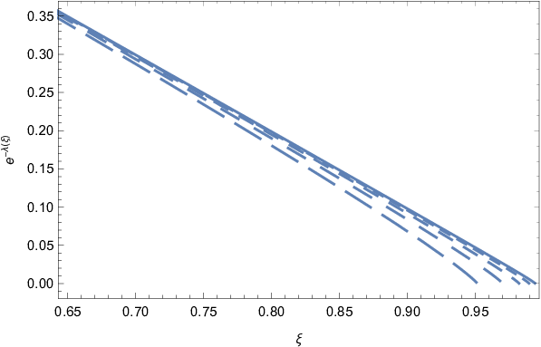
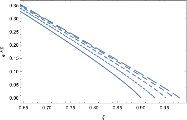
As a first example of numerical vacuum solutions in HMPG, we consider the case $V(\phi)=0$ . In order to numerically integrate the gravitational field equations Eqs. (63)-(67) we need to fix the initial values of the scalar field $\phi$ , and of its derivative at infinity, corresponding to the value $\xi=0$ of the dimensionless radial coordinate $\xi$ . As for the metric we assume that at infinity it is Minkowskian. Hence the nature of the central singularity in HMPG is essentially determined by the numerical values the field $\phi$ and its derivative $\phi^{\prime}$ takes at infinity. In order to investigate the effect of the initial conditions we consider two different classes of solutions. In the first class we assume that the initial value of the field at infinity is fixed, and we let its derivatives vary. For the second set of models we take the derivative of the scalar field as fixed at infinity, and we investigate the effects of the field variation on the geometry. The variations of the metric tensor coefficient $e^{\nu}$ for these two cases is presented in Figs. 1.

Refer to caption — Figure 1: Variation of the metric tensor components $e^{\nu}$ in the vacuum outside a spherically symmetric compact object in HMPG with a vanishing scalar field potential. Left figure: The initial value of scalar field, $\phi_{0}$ , is fixed at $\phi_{0}=1$ while the initial value of its derivative is taken to be: $u_{0}=4\times 10^{-9}$ (solid curve), $u_{0}=8\times 10^{-9}$ (dotted curve), $u_{0}=1.6\times 10^{-8}$ (short dashed curve), $u_{0}=3.2\times 10^{-8}$ (dashed curve), $u_{0}=6.4\times 10^{-8}$ (long dashed curve). Right figure: The initial value of the derivative of the scalar field, $u_{0}$ , is fixed at $u_{0}=5.12\times 10^{-7}$ while the initial value of the scalar field is taken to be: $\phi_{0}=0.5$ (solid curve), $\phi_{0}=1$ (dotted curve), $\phi_{0}=2$ (short dashed curve), $\phi_{0}=4$ (dashed curve), $\phi_{0}=8$ (long dashed curve).

As one can see from the figures describing the variation of $e^{\nu}$ , at fixed values of $\xi=\xi_{S}$ the metric becomes singular. The same effect can be also observed in the case of the evolution of $e^{-\lambda}$ , presented in Figs. 2. For both metric tensor coefficients a singular behavior does appear for a finite value of $\xi$ , indicating the formation of an outer apparent horizon, and of a black hole. However, the position of the outer apparent horizon $\xi_{S}$ covering the black hole depends on the initial values at infinity of the scalar field.

The variation of the effective mass of the black hole is represented in Figs. 3. As indicated by the figures, the mass of the black hole significantly increases as compared to its mass at infinity, where the effects of the scalar field are neglected. Hence, in HMPG the scalar field gives a significant contribution to the mass of the gravitating object.

The exact locations of the outer apparent horizon for HPMG with a vanishing scalar field potential are represented in Table 1 and 2, respectively.

$u_{0}$	$\xi_{S}$
$5\times 10^{-10}$	0.99856
$1\times 10^{-9}$	0.99781
$2\times 10^{-9}$	0.99641
$4\times 10^{-9}$	0.99391
$8\times 10^{-9}$	0.98956
$1.6\times 10^{-8}$	0.98219
$3.2\times 10^{-8}$	0.97020
$6.4\times 10^{-8}$	0.95155
$1.28\times 10^{-7}$	0.92393
$2.56\times 10^{-7}$	0.88450
$5.12\times 10^{-7}$	0.82693

Table 1: Values of

\xi=\xi_{S}

where the singularity occurs, corresponding to the radius of the outer apparent horizon, for fixed

\phi_{0}=1

and different values of

\phi^{\prime}(0)=u_{0}

for the case of the vanishing scalar field potential

V=0

$\phi_{0}$	$\xi_{S}$
0.5	0.77061
1	0.82693
2	0.86764
4	0.90060
8	0.92965
16	0.95335
32	0.97065
64	0.98219
128	0.98939
256	0.99366
512	0.99610

Table 2: Values of

\xi=\xi_{S}

where the singularity in the static vacuum field equations of HMPG occurs, for fixed

u_{0}=5.12\times 10^{-7}

and for different values of

\phi_{0}

in the case of the vanishing scalar field potential

V=0

As one can see from Table 1, for very small values of $u_{0}$ , the position of the outer apparent horizon of the HMPG black hole almost coincides with the Schwarzschild radius of the black hole $\xi_{S}=1$ . With the increase of $u_{0}$ there is a significant decrease in the numerical values of the metric singularity, which can reach values as low as 0.8 of the Schwarzschild radius, indicating that the presence of the scalar field pushes the outer apparent horizon towards the center of the black hole. A different trend can be observed from the numerical results presented in Table 2. For a fixed but small $u_{0}$ , the position of the outer apparent horizon is inversely proportional to the initial values of the scalar field. The outer apparent horizon of the black hole approaches the Schwarzschild radius for large initial values of the field, while small values of $\phi_{0}$ of the order of one lead to a significant decrease in the position of $\xi_{S}$ .

IV.1.1 Fitting of the numerical results

As a function of the initial conditions for the scalar field the expression of the outer apparent horizon of the black hole can be obtained as

\xi_{S}\left(\phi_{0},u_{0}\right)=1-148411\times\frac{u_{0}}{\phi_{0}}-2.737\times 10^{11}\times u_{0}^{2},

(85)

with an $R$ squared value of $R^{2}=0.99926$ . The comparison of the numerical results and of the fitting function is presented in Fig. 4.

We have also obtained numerical fits for the three functions, $M_{eff}(\xi)$ , $e^{\nu(\xi)}$ and $e^{-\lambda(\xi)}$ , for the same combination of parameters $\phi_{0},u_{0}$ as in Table 1 and Table 2.

For the mass function we consider a representation of the form

M_{eff}(\xi)=A_{M}+B_{M}\xi+C_{M}\xi^{2},

(86)

where we have further obtained the coefficients $A_{M}$ , $B_{M}$ , $C_{M}$ as functions $A_{M}=A_{M}\left(\phi_{0},u_{0}\right)$ , $B_{M}=B_{M}\left(\phi_{0},u_{0}\right)$ , and $C_{M}=C_{M}\left(\phi_{0},u_{0}\right)$ as given below,

$\displaystyle A_{M}$	$\displaystyle=$	$\displaystyle 1.00067+53919.2u_{0}-4814.28\times\phi_{0}u_{0}$	(87)
		$\displaystyle-3.34854\times 10^{10}\times u_{0}^{2}-\frac{2.72635\times 10^{9}u_{0}^{2}}{\phi_{0}^{2}}$
		$\displaystyle+\frac{6.44955\times 10^{9}\times u_{0}^{2}}{\phi_{0}},$

with an $R$ squared of $R^{2}=0.999998$ ,

$\displaystyle B_{M}$	$\displaystyle=$	$\displaystyle-213635u_{0}+\frac{23702.9u_{0}}{\phi_{0}}+18747.6\times\phi_{0}u_{0}$	(88)
		$\displaystyle+1.52191\times 10^{11}u_{0}^{2}+\frac{3.86999\times 10^{10}u_{0}^{2}}{\phi_{0}^{2}}$
		$\displaystyle-\frac{5.94209\times 10^{10}u_{0}^{2}}{\phi_{0}},$

with with $R^{2}=0.965492$ , and finally

$\displaystyle C_{M}$	$\displaystyle=$	$\displaystyle 639111u_{0}+\frac{25555.1u_{0}}{\phi_{0}}-39078.4\phi_{0}u_{0}$	(89)
		$\displaystyle-5.82573\times 10^{11}u_{0}^{2}-\frac{5.7583\times 10^{10}u_{0}^{2}}{\phi_{0}^{2}}$
		$\displaystyle+\frac{5.73072\times 10^{11}u_{0}^{2}}{\phi_{0}},$

with an $R$ squared of $R^{2}=0.990561$ , respectively.

For the metric tensor coefficient $e^{\nu(\xi)}$ , we consider a representation of the form

e^{\nu(\xi)}=A_{\nu}+B_{\nu}\xi+C_{\nu}\xi^{2},

(90)

where the coefficients $A_{\nu}$ , $B_{\nu}$ , and $C_{\nu}$ are given as functions of the initial values of the scalar field as

$\displaystyle A_{\nu}$	$\displaystyle=$	$\displaystyle 1.01476-165700.u_{0}+17233.5\phi_{0}u_{0}$	(91)
		$\displaystyle+9.14106\times 10^{10}u_{0}^{2}+\frac{7.59538\times 10^{9}u_{0}^{2}}{\phi_{0}^{2}}$
		$\displaystyle-\frac{3.95859\times 10^{10}u_{0}^{2}}{\phi_{0}},$

with an $R$ squared of $R^{2}=0.999985$ ,

$\displaystyle B_{\nu}$	$\displaystyle=$	$\displaystyle-0.995931+2.28588\times 10^{6}u_{0}-231896\phi_{0}u_{0}$	(92)
		$\displaystyle-1.36511\times 10^{12}u_{0}^{2}-\frac{1.13951\times 10^{11}u_{0}^{2}}{\phi_{0}^{2}}$
		$\displaystyle+\frac{1.01312\times 10^{12}u_{0}^{2}}{\phi_{0}},$

with $R^{2}=0.997263$ , and finally

$\displaystyle C_{\nu}$	$\displaystyle=$	$\displaystyle-1.54598\times 10^{6}u_{0}-\frac{255308u_{0}}{\phi_{0}}$	(93)
		$\displaystyle+120339\phi_{0}u_{0}+1.18476\times 10^{12}u_{0}^{2}$
		$\displaystyle+\frac{1.24333\times 10^{11}u_{0}^{2}}{\phi_{0}^{2}}-\frac{1.6744\times 10^{12}u_{0}^{2}}{\phi_{0}},$

with an $R$ squared of $R^{2}=0.997204$ .

For the metric tensor component $e^{-\lambda(\xi)}$ , we adopt the functional form

	$\displaystyle e^{-\lambda(\xi)}$	$\displaystyle=$	$\displaystyle 1-\xi M_{eff}(\xi)=1-(A_{M}+B_{M}\xi+C_{M}\xi^{2})$		(94)
		$\displaystyle=$	$\displaystyle 1+A_{\lambda}\xi+B_{\lambda}\xi^{2}+C_{\lambda}\xi^{3},$		(94)

where the coefficients $A_{\lambda}$ , $B_{\lambda}$ , $C_{\lambda}$ are given as functions of the initial conditions at infinity of the scalar field as

$\displaystyle A_{\lambda}$	$\displaystyle=$	$\displaystyle-0.933912-108822u_{0}+10973\phi_{0}u_{0}$	(95)
		$\displaystyle+4.6961\times 10^{10}u_{0}^{2}+\frac{6.11265\times 10^{9}u_{0}^{2}}{\phi_{0}^{2}}$
		$\displaystyle+\frac{1.81929\times 10^{10}u_{0}^{2}}{\phi_{0}},$

with an $R$ squared of $R^{2}=0.999976$ ,

$\displaystyle B_{\lambda}$	$\displaystyle=$	$\displaystyle-0.121357+357381u_{0}-41431\phi_{0}u_{0}$	(96)
		$\displaystyle-1.12908\times 10^{11}u_{0}^{2}-\frac{7.12164\times 10^{10}u_{0}^{2}}{\phi_{0}^{2}}$
		$\displaystyle-\frac{8.9032\times 10^{9}u_{0}^{2}}{\phi_{0}},$

with $R^{2}=0.981236$ , and

$\displaystyle C_{\lambda}$	$\displaystyle=$	$\displaystyle 0.0645491-777792u_{0}-\frac{36125u_{0}}{\phi_{0}}$	(97)
		$\displaystyle+59800.9\phi_{0}u_{0}+6.11368\times 10^{11}u_{0}^{2}$
		$\displaystyle+\frac{1.16131\times 10^{11}u_{0}^{2}}{\phi_{0}^{2}}-\frac{6.21693\times 10^{11}u_{0}^{2}}{\phi_{0}},$

with an $R$ squared of $R^{2}=0.961695$ , respectively.

IV.2 The Higgs-type potential: $V(\phi)=-\frac{\mu^{2}}{2}\phi^{2}+\frac{\varsigma}{4}\phi^{4}$

As another example of vacuum solutions of the gravitational field equations in HMPG we consider the case of the scalar field with Higgs-type potential,

V(\phi)=-\frac{\mu^{2}}{2}\phi^{2}+\frac{\varsigma}{4}\phi^{4},

(98)

where $\mu^{2}$ and $\varsigma$ are constants. The Higgs potential plays a fundamental role in particle physics, and by analogy with quantum field theoretical models we assume that $-\mu^{2}$ gives the mass of the scalar field particle associated to HMPG. The Higgs self-coupling constant $\varsigma$ takes the value $\varsigma\approx 1/8$ for the case of strong interactions Higgs. This value is obtained from the determination of the mass of the Higgs boson from accelerator experiments, but the self-interacting properties of the scalar field in HMPG may be very different than those suggested by QCD. By taking into account the new variable introduced in the present approach the scalar field potential can be written in a dimensionless form as

v(\phi)=\alpha\phi^{2}+\beta\phi^{4},

(99)

where

\alpha=-\frac{1}{4}\left(\frac{2GnM_{\odot}}{c^{2}}\right)^{2}\mu^{2},\quad\beta=\frac{1}{2}\left(\frac{2GnM_{\odot}}{c^{2}}\right)^{2}\varsigma.

(100)

The Higgs-type potential generates four-parameter ( $\alpha$ , $\beta$ , $\phi_{0}$ , $u_{0}$ ) classes of solutions of the static gravitational field equations in HMPG. However, in the following, we will restrict our analysis to the investigation of the role played by the constants $\alpha$ and $\beta$ of the potential in the formation of the event horizon of the black holes. Hence, we fix $\phi_{0}$ and $u_{0}$ , and vary the numerical values of $\alpha$ and $\beta$ . The variations with respect to $\xi$ of the metric tensor components and of the mass function are represented, for fixed values of $\phi_{0}$ and $u_{0}$ in Figs. 5 and 6, respectively.

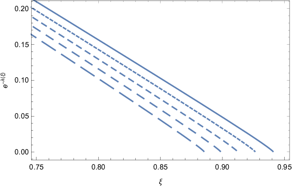
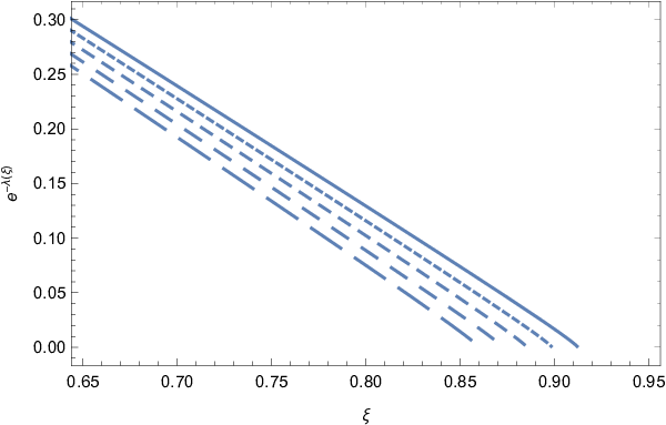
Similarly to the case of the zero scalar field potential, the metric tensor components become singular at finite values of the radial coordinate $\xi$ , indicating the presence of an event horizon, and the formation of a black hole. The position of the event horizon strongly depends on the model parameters, with this dependence exemplified in Table 3 and 4, respectively.

$\beta$	$\xi_{S}$
$2\times 10^{-10}$	0.97140
$3\times 10^{-10}$	0.95582
$4\times 10^{-10}$	0.94075
$5\times 10^{-10}$	0.92615
$6\times 10^{-10}$	0.91201
$7\times 10^{-10}$	0.89930
$8\times 10^{-10}$	0.88499
$9\times 10^{-10}$	0.87207

Table 3: Values of

\xi=\xi_{S}

where the singularity in the field equations occur, indicating the formation of an outer apparent horizon, for fixed

\phi_{0}=1

u_{0}=10^{-8}

\alpha=10^{-10}

and varying

\beta

in the case of the Higgs potential,

V=\alpha\phi^{2}+\beta\phi^{4}

$\alpha$	$\xi_{S}$
$-2\times 10^{-10}$	0.94075
$-3\times 10^{-10}$	0.91201
$-4\times 10^{-10}$	0.92615
$-5\times 10^{-10}$	0.89829
$-6\times 10^{-10}$	0.88498
$-7\times 10^{-10}$	0.87207
$-8\times 10^{-10}$	0.85952
$-9\times 10^{-10}$	0.84734

Table 4: Values of

\xi=\xi_{S}

where the singularity in the field equations occur, indicating the formation of an outer apparent horizon, for fixed

\phi_{0}=1

u_{0}=10^{-8}

\beta=10^{-10}

and varying

\alpha

in the case of the Higgs potential,

V=\alpha\phi^{2}+\beta\phi^{4}

The effective mass function $M(\xi)$ , represented in Fig. 7, shows an increase of the mass of the black hole while approaching the outer apparent horizon. The increase is strongly dependent on numerical values of the model parameters and, due to the contribution of the scalar field, can lead to a significant increase in the gravitational mass of the central object. In the considered examples this increase can be of the order of 20% as compared to the mass at infinity.

IV.2.1 Numerical fits of the solutions

We have also obtained numerical fits for the three functions, $M_{eff}(\xi)$ , $e^{\nu(\xi)}$ and $e^{-\lambda(\xi)}$ , for all the combination of parameters $\phi_{0}=\{0.5,0.6,0.7,0.8,0.9\}$ , $u_{0}=\{1,2,3,4,5\}\times 10^{-8}$ , $\alpha=\{1.0,1.5,2.0,2.5,3.0\}\times 10^{-10}$ , $\beta=\{1,2,3,4,5\}\times 10^{-10}$ .

For the mass function, we assume a general representation of the form

M_{eff}(\xi)=A_{MH}+B_{MH}\xi+C_{MH}\xi^{2}+D_{MH}\xi^{3},

(101)

where we further consider the coefficients $A_{MH}$ , $B_{MH}$ , $C_{MH}$ and $D_{MH}$ as functions $A_{MH}=A_{MH}\left(\phi_{0},u_{0},\alpha,\beta\right)$ , $B_{MH}=B_{MH}\left(\phi_{0},u_{0},\alpha,\beta\right)$ , $C_{MH}=C_{MH}\left(\phi_{0},u_{0},\alpha,\beta\right)$ , and $D_{MH}=D_{MH}\left(\phi_{0},u_{0},\alpha,\beta\right)$ , respectively. The explicit form of these coefficients is given below as

$\displaystyle A_{MH}$	$\displaystyle=$	$\displaystyle 1+6.04244\times 10^{7}\beta-3.82478\times 10^{6}u_{0}$	(102)
		$\displaystyle+\frac{1.024\times 10^{6}u_{0}}{\phi_{0}}+3.23921\times 10^{6}\phi_{0}u_{0}$
		$\displaystyle-1.09018\times 10^{8}\alpha+2.85266\times 10^{15}\alpha\beta,$

with an $R$ squared of $R^{2}=0.999961$ ,

$\displaystyle B_{MH}$	$\displaystyle=$	$\displaystyle 1.787\times 10^{7}\beta+337899u_{0}$	(103)
		$\displaystyle+\frac{159812u_{0}}{\phi_{0}}+159110\phi_{0}u_{0}-914980\alpha$
		$\displaystyle-4.13735\times 10^{16}\alpha\beta,$

with $R^{2}=0.997251$ ,

$\displaystyle C_{MH}$	$\displaystyle=$	$\displaystyle-4.65809\times 10^{7}\beta-468798u_{0}-\frac{310459.u_{0}}{\phi_{0}}$	(104)
		$\displaystyle-477549\phi_{0}u_{0}-8.95984\times 10^{6}\alpha$
		$\displaystyle+1.21263\times 10^{17}\alpha\beta,$

with $R^{2}=0.994383$ , and finally

$\displaystyle D_{MH}$	$\displaystyle=$	$\displaystyle 4.73217\times 10^{7}\beta+320946u_{0}+\frac{425716.u_{0}}{\phi_{0}}$	(105)
		$\displaystyle+701419.\phi_{0}u_{0}-6.8347\times 10^{6}\alpha$
		$\displaystyle-1.04108\times 10^{17}\alpha\beta,$

with an $R$ squared of $R^{2}=0.99634$ .

For the metric tensor coefficient $e^{\nu(\xi)}$ , we assume an analytical representation of the form

e^{\nu(\xi)}=A_{\nu H}+B_{\nu H}\xi+C_{\nu H}\xi^{2}+D_{\nu H}\xi^{3},

(106)

where we further consider the coefficients $A$ , $B$ , $C$ , $D$ as functions of the form $A_{\nu H}=A_{\nu H}(\phi_{0},u_{0},\alpha,\beta)$ , $B_{\nu H}=B_{\nu H}(\phi_{0},u_{0},\alpha,\beta)$ , $C_{\nu H}=C_{\nu H}(\phi_{0},u_{0},\alpha,\beta)$ , $D_{\nu H}=D_{\nu H}(\phi_{0},u_{0},\alpha,\beta)$ , with the explicit forms of these functions given below as

$\displaystyle A_{\nu H}$	$\displaystyle=$	$\displaystyle 1+3.74259\times 10^{7}\beta-4377.59u_{0}+\frac{22095.4u_{0}}{\phi_{0}}$	(107)
		$\displaystyle+57374.6\phi_{0}u_{0}+5.63505\times 10^{7}\alpha$
		$\displaystyle-1.60231\times 10^{17}\alpha\beta,$

with an $R$ squared of $R^{2}=0.999996$ ,

$\displaystyle B_{\nu H}$	$\displaystyle=$	$\displaystyle-1-3.99701\times 10^{7}\beta+3.93268\times 10^{6}u_{0}$	(108)
		$\displaystyle-\frac{858026u_{0}}{\phi_{0}}-3.0797\times 10^{6}\phi_{0}u_{0}$
		$\displaystyle+1.20215\times 10^{8}\alpha-6.73634\times 10^{16}\alpha\beta,$

with $R^{2}=0.999962$ ,

$\displaystyle C_{\nu H}$	$\displaystyle=$	$\displaystyle-1.69096\times 10^{7}\beta+1.42883\times 10^{6}u_{0}$	(109)
		$\displaystyle+\frac{282037u_{0}}{\phi_{0}}+14781.9\phi_{0}u_{0}-8.68885\times 10^{7}\alpha$
		$\displaystyle+1.51073\times 10^{17}\alpha\beta,$

with $R^{2}=0.99119$ , and finally

$\displaystyle D_{\nu H}$	$\displaystyle=$	$\displaystyle-2.6232\times 10^{7}\beta-1.209\times 10^{6}u_{0}$	(110)
		$\displaystyle-\frac{671312u_{0}}{\phi_{0}}-656553\phi_{0}u_{0}+7.44748\times 10^{7}\alpha$
		$\displaystyle-3.06922\times 10^{16}\alpha\beta,$

with an $R$ squared of $R^{2}=0.997681$ .

For the metric tensor coefficient of $e^{-\lambda(\xi)}$ , we adopt a functional representation of the form

$\displaystyle e^{-\lambda(\xi)}$	$\displaystyle=$	$\displaystyle 1-\xi M_{eff}(\xi)$	(111)
	$\displaystyle=$	$\displaystyle 1-(A_{MH}+B_{MH}\xi+C_{MH}\xi^{2}+D_{MH}\xi^{3})$
	$\displaystyle=$	$\displaystyle 1+A_{\lambda H}\xi+B_{\lambda H}\xi^{2}+C_{\lambda H}\xi^{3}+D_{\lambda H}\xi^{4},$

and we further consider the coefficients $A_{\lambda H}$ , $B_{\lambda H}$ , $C_{\lambda H}$ , $D_{\lambda H}$ as functions of $\phi_{0}$ and $u_{0}$ , respectively, so that $A_{\lambda H}=A_{\lambda H}(\phi_{0},u_{0},\alpha,\beta)$ , $B_{\lambda H}=B_{\lambda H}(\phi_{0},u_{0},\alpha,\beta)$ , $C_{\lambda H}=C_{\lambda H}(\phi_{0},u_{0},\alpha,\beta)$ , and $D_{\lambda H}=D_{\lambda H}(\phi_{0},u_{0},\alpha,\beta)$ , respectively. The explicit forms of these functions are given below as

$\displaystyle A_{\lambda H}$	$\displaystyle=$	$\displaystyle-1-4.49859\times 10^{7}\beta+4.09247\times 10^{6}u_{0}$	(112)
		$\displaystyle-\frac{966006u_{0}}{\phi_{0}}-3.19464\times 10^{6}\phi_{0}u_{0}$
		$\displaystyle+1.19154\times 10^{8}\alpha-5.17235\times 10^{16}\alpha\beta,$

with an $R$ squared of $R^{2}=0.99996$ ,

$\displaystyle B_{\lambda H}$	$\displaystyle=$	$\displaystyle-9.47158\times 10^{7}\beta-1.36178\times 10^{6}u_{0}$	(113)
		$\displaystyle-\frac{530466u_{0}}{\phi_{0}}-626997\phi_{0}u_{0}$
		$\displaystyle-3.64982\times 10^{7}\alpha+2.68594\times 10^{17}\alpha\beta,$

with $R^{2}=0.993292$ ,

$\displaystyle C_{\lambda H}$	$\displaystyle=$	$\displaystyle 1.78597\times 10^{8}\beta+1.6928\times 10^{6}u_{0}$	(114)
		$\displaystyle+\frac{1.09374\times 10^{6}u_{0}}{\phi_{0}}+1.71268\times 10^{6}\phi_{0}u_{0}$
		$\displaystyle+5.07146\times 10^{7}\alpha-4.84226\times 10^{17}\alpha\beta,$

with $R^{2}=0.997681$ , and finally

$\displaystyle D_{\lambda H}$	$\displaystyle=$	$\displaystyle-0.0292287-4.65552\times 10^{7}\beta-618525u_{0}$	(115)
		$\displaystyle-\frac{932125u_{0}}{\phi_{0}}-1.6095\times 10^{6}\phi_{0}u_{0}$
		$\displaystyle+1.1466\times 10^{8}\alpha-3.58837\times 10^{16}\alpha\beta,$

with an $R$ squared of $R^{2}=0.995662$ .

V Thermodynamics of HMPG black holes

In the present analysis of the vacuum field equations in HMPG we have assumed that the mass function and lapse function $e^{\nu}$ depend only on the radial coordinate. Hence the spacetime is static and a timelike Killing vector $t^{\mu}$ exists Wald; Kunst. The definition of the surface gravity $\tilde{\kappa}$ for a static black hole that possesses a Killing horizon is given by Wald; Kunst

t^{\mu}\nabla_{\mu}t^{\nu}=t^{\nu}\tilde{\kappa}.

(116)

In the case of a static, spherically symmetric geometry that can be written as

ds^{2}=-\tilde{\sigma}^{2}(r)f(r)c^{2}dt^{2}+\frac{dr^{2}}{f(r)}+r^{2}d\Omega^{2},

(117)

by adopting a suitable normalized Killing vector $t^{\mu}=\left(1/\tilde{\sigma}_{\infty},0,0,0\right)$ , the surface gravity of the black hole can be obtained as Kunst

\tilde{\kappa}=\left(\frac{\tilde{\sigma}_{hor}}{\tilde{\sigma}_{\infty}}\right)\frac{c^{4}}{4GM_{hor}}\left.\left[1-\frac{2GM^{\prime}(r)}{c^{2}}\right]\right|_{hor},

(118)

where the subscript hor indicates that the evaluation of all physical quantities must be performed on the outer apparent horizon. For $\sigma\equiv 1$ , and $M={\rm constant}$ , we reobtain the well-known result of the surface gravity of a Schwarzschild black hole, $\tilde{\kappa}=c^{4}/4GM_{hor}$ Wald. The temperature $T_{BH}$ of the black hole is defined as

T_{BH}=\frac{\hbar}{2\pi ck_{B}}\tilde{\kappa},

(119)

where $k_{B}$ is Boltzmann’s constant. In the dimensionless variables introduced in Eq. (III.3) we obtain the temperature of the black hole as

T_{BH}=T_{H}\frac{1}{M_{eff}\left(\xi_{S}\right)}\left.\left(1+\xi^{2}\frac{dM_{eff}\left(\xi\right)}{d\xi}\right)\right|_{\xi=\xi_{S}},

(120)

where

T_{H}=\frac{\hbar c^{3}}{8\pi Gk_{B}nM_{\odot}}.

(121)

By taking into account the representation of the effective mass as given by Eqs. (86) and (101), we obtain for the temperature of a HMPG black hole, the expression

	$\displaystyle T_{BH}\left(\xi_{S}\right)$	$\displaystyle=$	$\displaystyle T_{H}\left.\frac{1+\xi^{2}\left(B+2C\xi+3D\xi^{2}\right)}{A+B\xi+C\xi^{2}+D\xi^{3}}\right\|_{\xi=\xi_{S}}$		(122)
		$\displaystyle=$	$\displaystyle T_{H}\left.\theta\left(\xi\right)\right\|_{\xi=\xi_{S}}.$		(122)

For the zero potential case $V=0$ the variation of the horizon temperature of HMPG black holes is represented in Fig. 8. Explicit numerical values of the $T_{BH}\left(\xi_{S}\right)/T_{H}$ ratio are presented in Table 5.

$\phi_{0}$ / $u_{0}$	$0.15$	$0.225$	$0.3375$
$2.2\times 10^{-10}$	1.0004	1.00038	1.00035
$1.76\times 10^{-9}$	1.00316	1.00298	1.00273
$1.408\times 10^{-8}$	1.01904	1.01825	1.017
$1.1264\times 10^{-7}$	1.05587	1.0653	1.06176

Table 5: Selected numerical values of the black hole temperature

T_{BH}\left(\xi_{S}\right)/T_{H}

in the absence of a scalar field potential,

V=0

, for

\phi_{0}=\{0.15,0.225,0.3375\}

and

u_{0}=\{2.2\times 10^{-10},1.76\times 10^{-9},1.408\times 10^{-8},1.1264\times 10^{-8}\}

The specific heat $C_{BH}$ of the black hole can be obtained as

	$\displaystyle C_{BH}$	$\displaystyle=$	$\displaystyle\frac{dM}{dT_{BH}}=\left.\frac{dM}{dr}\frac{dr}{dT_{BH}}\right\|_{r=r_{hor}}$		(123)
		$\displaystyle=$	$\displaystyle\frac{nM_{\odot}}{T_{H}}\left.\frac{dM_{eff}\left(\xi\right)}{d\xi}\frac{d\xi}{d\theta}\right\|_{\xi=\xi_{S}}.$		(123)

Hence for the specific heat of a black hole in HMPG we obtain the general expression

C_{BH}\left(\xi_{S}\right)=C_{H}\frac{\left[B+\xi(2C+3D\xi)\right]\left\{A+\xi\left[B+\xi\left(C+D\xi\right)\right]\right\}^{2}}{B\left[2A\xi+4\xi^{3}\left(C+2D\xi\right)-1\right]+\xi\left[C\left(6A\xi+6D\xi^{4}-2\right)+3D\xi\left(4A\xi+D\xi^{4}-1\right)+2C^{2}\xi^{3}\right]+B^{2}\xi^{2}},

(124)

where we have denoted $C_{H}=nM_{\odot}/T_{H}$ . The variation of the specific heat of the HMPG black holes as a function of the dimensionless horizon radius is represented, for the zero potential case $V=0$ , in Fig. 9. Exact numerical values of the ratio $C_{BH}\left(\xi_{S}\right)/C_{H}$ for different values of $\phi_{0}$ and $u_{0}$ are presented in Table 6.

$\phi_{0}$ / $u_{0}$	$0.15$	$0.225$	$0.3375$
$2.2\times 10^{-10}$	0.435307	0.435248	0.43189
$1.76\times 10^{-9}$	0.43887	0.438458	0.438062
$1.408\times 10^{-8}$	0.475718	0.472819	0.470153
$1.1264\times 10^{-7}$	0.68967	0.638562	0.619363

Table 6: Numerical values of the specific heat

C_{BH}\left(\xi_{S}\right)/C_{H}

of a HMPG black hole in the absence of a scalar field potential,

V=0

, for

\phi_{0}=\{0.15,0.225,0.3375\}

and

u_{0}=\{2.2\times 10^{-10},1.76\times 10^{-9},1.408\times 10^{-8},1.1264\times 10^{-8}\}

The entropy $S_{BH}$ of the black hole is given by

\displaystyle S_{BH}

\displaystyle=

\displaystyle\int_{r_{in}}^{r_{hor}}{\frac{dM}{T_{BH}}}=\int_{r_{in}}^{r_{hor}}{\frac{1}{T_{BH}}\frac{dM}{dr}dr},

(125)

or, equivalently,

\displaystyle S_{BH}\left(\xi_{S}\right)=C_{H}\int_{0}^{\xi_{S}}{\frac{1}{\theta\left(\xi\right)}\frac{dM_{eff}\left(\xi\right)}{d\xi}d\xi}.

(126)

The variation as a function of the dimensionless horizon radius $\xi_{S}$ of the entropy of the HMPG black holes is represented, for the zero potential case $V=0$ , in Fig. 10. Selected values of the ratio $S_{BH}\left(\xi_{S}\right)/C_{H}$ for different values of $\phi_{0}$ and $u_{0}$ are presented in Fig. 7.

$\phi_{0}$ / $u_{0}$	$0.15$	$0.225$	$0.3375$
$2.2\times 10^{-10}$	$2.414\times 10^{-4}$	$2.267\times 10^{-4}$	$2.076\times 10^{-4}$
$1.76\times 10^{-9}$	$1.905\times 10^{-3}$	$1.790\times 10^{-3}$	$1.641\times 10^{-3}$
$1.408\times 10^{-8}$	$1.384\times 10^{-2}$	$1.303\times 10^{-2}$	$1.199\times 10^{-2}$
$1.126\times 10^{-7}$	$8.938\times 10^{-2}$	$8.181\times 10^{-2}$	$7.299\times 10^{-2}$

Table 7: Numerical values of the entropy

S_{BH}\left(\xi_{S}\right)/C_{H}

of a HMPG black hole in the absence of a scalar field potential,

V=0

, for

\phi_{0}=\{0.15,0.225,0.3375\}

and

u_{0}=\{2.2\times 10^{-10},1.76\times 10^{-9},1.408\times 10^{-8},1.1264\times 10^{-8}\}

The black hole luminosity due to the Hawking evaporation can be obtained as

L_{BH}=-\frac{dM}{dt}=-\sigma A_{BH}T_{BH}^{4},

(127)

where $\sigma$ is a model dependent parameter, and $A_{BH}=4\pi r_{hor}^{2}$ is the area of the event horizon. Hence for the black hole evaporation time $\tau$ we find

\displaystyle\hskip-22.76228pt\tau

\displaystyle=

\displaystyle\int_{t_{in}}^{t_{fin}}{dt}=-\frac{1}{4\pi\sigma}\int_{t_{in}}^{t_{fin}}{\frac{dM}{r_{hor}^{2}T_{BH}^{4}}},

(128)

or equivalently,

\displaystyle\tau\left(\xi_{S}\right)=-\tau_{H}\int_{0}^{\xi_{S}}{\frac{1}{\xi^{2}\theta^{4}\left(\xi\right)}\frac{dM_{eff}\left(\xi\right)}{d\xi}d\xi},

(129)

where we have denoted

\tau_{H}=\frac{c^{4}}{8\pi G^{2}\sigma nM_{\odot}T_{BH}^{4}}.

(130)

The variation of the Hawking evaporation time as a function of the dimensionless horizon radius $\xi_{S}$ of the HMPG black holes is represented, for the zero potential case $V=0$ , in Fig. 11. Explicit exact numerical values of the evaporation time $\tau_{BH}\left(\xi_{S}\right)/\tau_{H}$ are presented, for different values of $\phi_{0}$ and $u_{0}$ , in Table 8.

$\phi_{0}$ / $u_{0}$	$0.15$	$0.225$	$0.3375$
$2.2\times 10^{-10}$	$2.421\times 10^{-4}$	$2.273\times 10^{-4}$	$2.082\times 10^{-4}$
$1.76\times 10^{-9}$	$1.938\times 10^{-3}$	$1.819\times 10^{-3}$	$1.666\times 10^{-3}$
$1.408\times 10^{-8}$	$1.513\times 10^{-2}$	$1.419\times 10^{-2}$	$1.299\times 10^{-2}$
$1.126\times 10^{-7}$	$1.444\times 10^{-1}$	$1.222\times 10^{-1}$	$1.058\times 10^{-1}$

Table 8: Numerical values of the evaporation time

\tau_{BH}\left(\xi_{S}\right)/\tau_{H}

of a HMPG black hole in the absence of a scalar field potential,

V=0

, for

\phi_{0}=\{0.15,0.225,0.3375\}

and

u_{0}=\{2.2\times 10^{-10},1.76\times 10^{-9},1.408\times 10^{-8},1.1264\times 10^{-8}\}

VI Discussions and final remarks

In the present paper, we have investigated the possible existence of black hole type structures in the framework of the HMPG theory, by considering the simplest case, corresponding to a vacuum static and spherically symmetric geometry. Even within this simple theoretical model the field equations of the theory become extremely complicated, and therefore in order to obtain solutions of the field equations one must resort to numerical methods. To this effect, we have reformulated the static spherically symmetric Einstein field equations in their scalar-tensor representation in a dimensionless form, and introduced the inverse of the radial coordinate as the independent variable. This representation allows an easier numerical integration procedure, which also requires fixing the numerical values of the scalar field, of its derivative, and of the effective mass at infinity. The appearance of a singular behavior in the field equations or, more exactly, in the behavior of the metric tensor coefficients, is interpreted as indicating the presence of an event horizon and, consequently, of a black hole type object. The mass of the black hole is given by the effective mass of the model, which represents the total contribution of the ordinary mass of the black hole plus the contribution from the scalar field.

We have considered the solutions of the gravitational field equations of the HMPG theory for two choices of the scalar field potential $V\left(\phi\right)$ , corresponding to the cases of the vanishing potential, and of the Higgs-type potential, respectively. In both cases our results indicate the formation of an event horizon, and consequently of black holes. The position of the event horizon depends on the values of the scalar field and of its derivative at infinity (the initial conditions), indicating the existence of a complex relation between scalar field and black hole properties. For the zero potential case and for particular scalar field initial conditions the event horizon can be located at distances of the order of 0.7 of the standard Schwarzschild radius, indicating the formation of more compact black holes as compared to standard general relativity. In the case of the Higgs-type potential the position of the event horizon is also strongly dependent on the parameters $\alpha$ and $\beta$ of the potential, indicating a multi-parametric dependence of the black hole properties. In all the cases studied it turns out that the numerical results can be fitted well by some simple analytical functions. In the zero potential case the metric function $e^{\nu(r)}$ can be described by a function of the type $e^{\nu}=1-B/r-C/r^{2}+D$ , with $A,B,C,D$ constants that depend on the initial conditions at infinity. The metric tensor component $e^{-\lambda}$ also contains a term proportional to $1/r^{3}$ . Similar simple analytic representations can describe the numerical results for the case of the Higgs-type potential. These analytical representations are extremely useful in the study of the thermodynamic properties of the HMPG black holes, as well as the dynamics and motion of matter particles around them. In particular, they may be used for the study of the electromagnetic properties of accretion disks that form around black holes, and which could allow discriminating this type of theoretical objects from their general relativistic counterparts, and for obtaining some constraints on the model parameters.

We have also investigated in detail the thermodynamic properties of the obtained numerical black hole solutions. One of the essential and interesting physical properties of black holes is their Hawking temperature. As compared to the standard general relativistic Hawking temperature, the horizon temperature of the HMPG black holes shows a strong dependence on the initial conditions at infinity, and the properties of the scalar field potential. As one can see from Fig. 8, a decrease in the horizon radius leads to a higher black hole temperature, which, in the case of the specific initial conditions considered in Fig. 8, is of the order of 10%, as compared to the standard general relativistic case. Similar effects appear for the specific heat, entropy and evaporation time of the HMPG black holes, all these quantities being strongly dependent on the initial conditions of the scalar field at infinity. In particular, the black hole evaporation times may be very different in HMPG as compared to standard general relativity. Of course our results on the thermodynamics of black holes, obtained for the zero potential case and for a limited set of initial conditions at infinity may be considered on qualitative nature only. But even at this level they indicate the complexity of the behavior of the HMPG black holes, and of the interesting physics related to them.

Black hole solutions are also well known in standard scalar field models. For a nonminimally coupled scalar field such exact analytical solutions have been obtained and studied a long time ago in Fisher; Bergmann; Newman; Bron; Sol; Tur (for a recent review nonsingular static, spherically symmetric solutions of general relativity with minimally coupled scalar fields see Bronrev). These solutions have been generally obtained in the Einstein frame, in which there is no coupling between the scalar field and the Ricci scalar. On the other hand because of the specific coupling between the scalar field and the Ricci scalar, the HMPG theory appears to be naturally formulated in the Jordan frame. Despite its superficial resemblance with the Brans-Dicke theory with coupling $w=-3/2$ , there are fundamental differences between the HMPG theory and scalar field models in the Einstein or Jordan frames. One such important difference appears in the zero potential case. While in the standard scalar field models the solutions with zero potential have in general no horizons, our investigations show that this is generally not the case in the HMPG theory, where even in the zero potential case the formation of ordinary black holes occur. In the standard scalar field models such a situation may occur for solutions admitting a conformal continuation, meaning that a singularity in the Einstein-frame manifold maps to a regular surface in the Jordan frame, and the solution is then continued beyond this surface Bronn1.

All possible types of spacetime causal structures that can appear in static, spherically symmetric configurations of a self-gravitating minimally coupled scalar field $\phi$ in general relativity, with an arbitrary potential $V(\phi)$ , were considered in Bronn2. It was first shown that a variable scalar field does not modify the possible structures with a constant scalar field. Moreover, in general relativistic scalar field models with arbitrary $V(\phi)$ there are no regular black holes with flat or AdS asymptotics. It also follows that the possible globally regular, asymptotically flat solutions are solitons with a regular center, without horizons and with at least partly negative potentials $V(\phi)$ . For a similar discussion of higher dimensional models see Bronn3. These results cannot be recovered in HMPG theory, in which in the case of Higgs-like potentials black hole solutions presenting an event horizon exist. In fact our numerical investigations did not reveal the presence of any globally regular solution.

An important result in black hole physics is the no-hair theorem Bek; Bek1; Adler; Bek2, stating that asymptotically flat black holes cannot possess external nontrivial scalar fields with non-negative field potential $V(\phi)$ . The results obtained in the present paper indicate that the no-hair theorem in its standard formulation cannot be extended to HMPG theory. All the considered black hole solutions are asymptotically flat, and scalar fields with positive potentials exist around them. However, the question if such structures result from a particular choice of the scalar field potentials and of the model parameters, or they are intrinsic properties of the theory deserves further investigation.

HMPG black holes may present a much richer theoretical structure, properties and variability, associated with an equally rich external dynamics, as compared with the standard general relativistic black holes. These properties are related to the presence of the intricate coupling between the scalar field, geometry and matter, which leads to very complex, strongly nonlinear, field equations. These new effects can also lead to some specific astrophysical signatures and imprints, whose observational detection could lead to new perspectives in gravitational physics and astrophysics. The possible astrophysical/observational implications of the existence of HMPG black holes will be considered in a future publication.

Acknowledgments

B.D. acknowledges financial support from PNIII STAR ACRONIM ASTRES: Centre of Competence For Planetary Sciences, Nr. 118/14.11.2016. F.S.N.L. acknowledges financial support of the Fundação para a Ciência e Tecnologia through the research grants No. UID/FIS/04434/2013, No. PEst-OE/FIS/UI2751/2014 and No. PTDC/FIS-OUT/29048/2017. T.H. would like to thank the Yat-Sen School of the Sun Yat-Sen University in Guangzhou, P. R. China, for the kind hospitality offered during the preparation of this work.

References

(1) A. G. Riess et al., Astron. J. 116, 1009 (1998).
(2) S. Perlmutter et al., Astrophys. J. 517, 565 (1999).
(3) R. A. Knop et al., Astrophys. J. 598, 102 (2003).
(4) R. Amanullah et al., Astrophys. J. 716, 712 (2010).
(5) D. H. Weinberg, M. J. Mortonson, D. J. Eisenstein, C. Hirata, A. G. Riess, and E. Rozo, Physics Reports 530, 87 (2013).
(6) S. Weinberg, Reviews of Modern Physics 61, 1 (1989).
(7) J. M. Overduin and P. S. Wesson, Physics Reports 402, 267 (2004).
(8) H. Baer, K.-Y. Choi, J. E. Kim, and L. Roszkowski, Physics Reports 555, 1 (2015).
(9) P. J. E. Peebles and B. Ratra, Rev. Mod. Phys. 75, 559 (2003).
(10) T. Padmanabhan, Phys. Repts. 380, 235 (2003).
(11) R. Caldwell, R. Dave and P. J. Steinhardt, Phys. Rev. Lett. 80, 1582 (1998).
(12) S. Tsujikawa, Class. Quant. Grav. 30, 214003 (2013).
(13) H. A. Buchdahl, Month. Not. R. Astron. Soc. 150, 1 (1970).
(14) J. D. Barrow and A. C. Ottewill, J. Phys. A: Math. Gen. 16, 2757 (1983).
(15) C. G. Boehmer, T. Harko, and F. S. N. Lobo, Astropart. Phys. 29, 386 (2008).
(16) O. Bertolami, C. G. Boehmer, T. Harko and F. S. N. Lobo, Phys. Rev. D 75, 104016 (2007).
(17) T. Harko, F. S. N. Lobo, S. Nojiri and S. D. Odintsov, Phys. Rev. D 84, 024020 (2011).
(18) S. M. Carroll, V. Duvvuri, M. Trodden and M. S. Turner, Phys. Rev. D 70, 043528 (2004).
(19) S. Nojiri and S. D. Odintsov, Int. J. Geom. Meth. Mod. Phys. 4, 115 (2007).
(20) F. S. N. Lobo, The dark side of gravity: Modified theories of gravity, “Dark Energy-Current Advances and Ideas”, 173-204 (2009), Research Signpost, ISBN 978-81-308-0341-8 [arXiv:0807.1640 [gr-qc]].
(21) A. De Felice and S. Tsujikawa, Living Rev. Rel. 13, 3 (2010).
(22) T. P. Sotiriou and V. Faraoni, Rev. Mod. Phys. 82, 451 (2010).
(23) S. Capozziello and M. De Laurentis, Phys. Rept. 509, 167 (2011).
(24) S. Nojiri and S. D. Odintsov, Phys. Rept. 505, 59 (2011).
(25) K. Bamba, S. Capozziello, S. Nojiri and S. D. Odintsov, Astrophys. Space Sci. 342, 155 (2012).
(26) P. Avelino, et al, Symmetry 8, 7 (2016).
(27) S. Nojiri, S. D. Odintsov and V. K. Oikonomou, Phys. Rept. 692, 1 (2017).
(28) G. J. Olmo, Int. J. Mod. Phys. D 20, 413 (2011).
(29) T. Harko, T. S. Koivisto, F. S. N. Lobo and G. J. Olmo, Phys. Rev. D 85, 084016 (2012).
(30) S. Capozziello, T. Harko, F. S. N. Lobo and G. J. Olmo, Int. J. Mod. Phys. D 22, 1342006 (2013).
(31) L. Amendola, K. Enqvist, and T. Koivisto, Phys. Rev. D 83, 044016 (2011).
(32) T. S. Koivisto, D. F. Mota and M. Sandstad, Novel aspects of C-theories in Cosmology, arXiv:1305.4754 [astro-ph.CO].
(33) C. G. Böhmer and N. Tamanini, Phys. Rev. D 87, 084031 (2013).
(34) C. G. Böhmer, F. S. N. Lobo and N. Tamanini, Phys. Rev. D 88, 104019 (2013).
(35) S. Capozziello, T. Harko, T. S. Koivisto, F. S. N. Lobo, and G. J. Olmo, JCAP 04, 011 (2013).
(36) S. Carloni, T. S. Koivisto, and F. S. N. Lobo, Phys. Rev. D 92, 064035 (2015).
(37) N. A. Lima, Phys. Rev. D 89, 083527 (2014).
(38) N. A. Lima and V. Smer-Barreto, Astrophys. Journal 818, 186 (2016).
(39) I. Leanizbarrutia, F. S. N. Lobo, and D. Sáez-Gómez, Phys. Rev. D 95, 084046 (2017).
(40) J. L. Rosa, S. Carloni, J. P. S. Lemos, and F. S. N. Lobo, Phys. Rev. D 95, 124035 (2017).
(41) M. V. dos Santos, J. S. Alcaniz, D. F. Mota, and S. Capozziello, Phys. Rev. D 97, 104010 (2018).
(42) J. Santos, M. J. Reboucas, and A. F. F. Teixeira, T Eur. Phys. J. C 78, 567 (2018).
(43) S. Capozziello, T. Harko, T. S. Koivisto, F. S. N. Lobo, and G. J. Olmo, JCAP 07, 024 (2013).
(44) S. Capozziello, T. Harko, T. S. Koivisto, F. S. N. Lobo, and G. J. Olmo, Astroparticle Physics 50-52C, 65 (2013).
(45) S. Capozziello, T. Harko, F. S. N. Lobo, G. J. Olmo and S. Vignolo, Int. J. Geom. Meth. Mod. Phys. 11, 1450042 (2014).
(46) S. Capozziello, T. Harko, T. S. Koivisto, F. S. N. Lobo and G. J. Olmo, Phys. Rev. D 86, 127504 (2012).
(47) J. L. Rosa, J. P. S. Lemos, and F. S. N. Lobo, Phys. Rev. D 98, 064054 (2018).
(48) B. Danil $\breve{\mathrm{a}}$ , T. Harko, F. S. N. Lobo, and M. K. Mak, Phys. Rev. D 95, 044031 (2017).
(49) S. Capozziello, T. Harko, T. S. Koivisto, F. S. N. Lobo, and G. J. Olmo, Universe 1, 199 (2015).
(50) T. Harko and F. S. N. Lobo, Extensions of $f(R)$ Gravity: Curvature-Matter Couplings and Hybrid Metric-Palatini Theory, Cambridge University Press, Cambridge, UK, 2018
(51) K. Schwarzschild, Sitzungsberichte der Deutschen Akademie der Wissenschaften zu Berlin, Klasse fur Mathematik, Physik, und Technik (1916), 189 (1916).
(52) D. Kramer, H. Stephani, M. MacCallum and E. Herlt, Exact solutions of Einstein’s field equations, Cambridge, Cambridge University Press, UK, 1980
(53) C. S. J. Pun, Z. Kovács, and T. Harko, Phys. Rev. D 78, 024043 (2008).
(54) T. Harko, Z. Kovács, and F. S. N. Lobo, Phys. Rev. D 78, 084005 (2008).
(55) C. S. J. Pun, Z. Kovács, and T. Harko, Phys. Rev. D 78, 084015 (2008).
(56) T. Harko, Z. Kovács, and F. S. N. Lobo, Phys. Rev. D 78, 084005 (2008).
(57) T. Harko, Z. Kovács, and F. S. N. Lobo, Phys. Rev. D 79, 064001 (2009).
(58) T. Harko, Z. Kovács, and F. S. N. Lobo, Phys. Rev. D80, 044021 (2009).
(59) T. Harko, Z. Kovács, and F. S. N. Lobo, Class. Quant. Grav. 27, 105010 (2010).
(60) T. Harko, Z. Kovács, and F. S. N. Lobo, Class. Quant. Grav. 28, 165001 (2011).
(61) B. D $\breve{\mathrm{a}}$ nil $\breve{\mathrm{a}}$ , T. Harko, and Z. Kovács, Eur. Phys. J. C 75, 203 (2015).
(62) Y. Ni, M. Zhou, A. Cardenas-Avendano, C. Bambi, C. A. R. Herdeiro, and E. Radu, JCAP 1607, 049 (2016).
(63) Y. Ni, J. Jiang, and C. Bambi, JCAP 1609, 014 (2016).
(64) C. Bambi, Z. Cao, and L. Modesto, Phys. Rev. D 95, 064006 (2017).
(65) H. Zhang, M. Zhou, C. Bambi, B. Kleihaus, J. Kunz, and E. Radu, Phys. Rev. D 95, 104043 (2017).
(66) Y. Zhang, M. Zhou, and C. Bambi, Eur. Phys. J. C 78, 376 (2018).
(67) S. Nampalliwar, C. Bambi, K. Kokkotas, and R. Konoplya, Phys. Lett. B781, 626 (2018).
(68) C. Bambi, Rev. Mod. Phys. 89, 025001 (2017).
(69) K. A. Bronnikov, H. Dehnen, and V. N. Melnikov, Phys. Rev. D 68, 024025 (2003).
(70) T. Harko and M. K. Mak, Phys. Rev. D 69, 064020 (2004).
(71) T. Harko and M. K. Mak, Annals of Physics (New York) 319, 471 (2005).
(72) T. Harko and V. S. Sabau, Phys. Rev. D77, 104009 (2008).
(73) C. Bambi, D. Rubiera-Garcia, and Y. Wang, Phys. Rev. D 94, 064002 (2016).
(74) C. Bambi, L. Modesto, and Y. Wang, Phys. Lett. B 764, 306 (2017).
(75) P. Li, X.-Z. Li, and P. Xi, Phys. Rev. D 93, 064040 (2016).
(76) K. Meng and J. Li, Europhysics Letters 116, 10005 (2016).
(77) J. A. R. Cembranos and J. G. Valcarcel, JCAP 1701, 014 (2017).
(78) Y. Heydarzade and F. Darabi, Phys. Lett. B 771, 365 (2017).
(79) L. Heisenberg, R. Kase, M. Minamitsuji, and S. Tsujikawa, Phys. Rev. D 96, 084049 (2017).
(80) C.-Y. Chen, M. Bouhmadi-López, and P. Chen, Eur. Phys. J. C 78, 59 (2018).
(81) F. Filippini and G. Tasinato, Journal of Cosmology and Astroparticle Physics 01, 033 (2018).
(82) M. E. Abishev, K. A. Boshkayev, and V. D. Ivashchuk, The European Physical Journal C 77, 180 (2017).
(83) R. A. Rosen, Journal of High Energy Physics 2017, 206 (2017).
(84) J. Ponce de Leon, Phys. Rev. D 95, 124015 (2017).
(85) C. Stelea, Phys. Rev. D 97, 024044 (2018).
(86) S. H. Hendi, B. Eslam Panah, and S. Panahiyan, Fortschr. Phys. 66, 1800005 (2018).
(87) S. H. Hendi, S. Panahiyan, and B. Eslam Panah, JHEP 01, 129 (2016).
(88) S. H. Hendi, B. Eslam Panah, and S. Panahiyan, Class. Quantum Grav. 33, 235007 (2016).
(89) S. H. Hendi, G. -Q. Li, J. -X. Mo, S. Panahiyan, and B. Eslam Panah, Eur. Phys. J. C 76, 571 (2016).
(90) G. Antoniou, A. Bakopoulos, and P. Kanti, Phys. Rev. Lett. 120, 131102 (2018).
(91) L. Heisenberg and S. Tsujikawa, Phys. Lett. B 780, 638 (2018).
(92) F. Herrera and Y. Vásquez, Phys. Lett. B 782, 305 (2018).
(93) S. Çikintog̃lu, Phys. Rev. D 97, 044040 (2018).
(94) S. H. Hendi, B. Eslam Panah, S. Panahiyan, and M. Momennia, Eur. Phys. J. C 77, 647 (2017).
(95) B. Eslam Panah, S. H. Hendi, S. Panahiyan, and M. Hassaine, Phys. Rev. D 98, 084006 (2018).
(96) D. Zwillinger, Handbook of Differential equations, Academic Press, Third edition, 1989
(97) P. G. Bergmann, Int. J. Theoret. Phys. 1, 25 (1968).
(98) R. V. Wagoner, Phys. Rev. D 1, 3209 (1970).
(99) K. Nordtvedt, Jr., Astrophys. J. 161, 1059 (1970).
(100) C. Brans and R. H. Dicke, Phys. Rev. 124, 925(1961).
(101) R. H. Dicke, Phys. Rev. 125, 2163 (1962).
(102) G. Aad et al. [ATLAS and CMS Collaborations], Phys. Rev. Lett. 114, 191803 (2015).
(103) R. M. Wald, General Relativity, University of Chicago Press, Chicago, 1984
(104) M. Pielahn, G. Kunstatter, and A. B. Nielsen, Phys. Rev. D 84, 104008 (2011).
(105) I. Z. Fisher, Zh. Eksp. Teor. Fiz. 18, 636 (1948).
(106) O. Bergmann and R. Leipnik, Phys. Rev. 107, 1157 (1957).
(107) A. I. Janis, E. T. Newman, and J. Winicour, Phys. Rev. Lett. 20, 878 (1968).
(108) K. A. Bronnikov, Acta Phys. Pol. B 4, 251 (1973).
(109) D. A. Solovyev and A. N. Tsirulev, Class. Quantum Grav. 29, 055013 (2012).
(110) B. Turimov, B. Ahmedov, M. Koloŝ, and Z. Stuchlik, Phys. Rev. D 98, 084039 (2018).
(111) K. A. Bronnikov, Particles 1, 56 (2018).
(112) K. A. Bronnikov, J. Math. Phys. 43, 6096 (2002).
(113) K. A. Bronnikov, Phys. Rev. D 64, 064013 (2001).
(114) K. A. Bronnikov, S. B. Fadeev, and A. V. Michtchenko, Gen. Rel. Grav. 35, 505 (2003).
(115) J. D. Bekenstein, Phys. Rev. D 5, 1239 (1972).
(116) J. D. Bekenstein, Phys. Rev. D 5, 2403 (1972).
(117) S. Adler and R. B. Pearson, Phys. Rev. D 18, 2798 (1978).
(118) J. D. Bekenstein, Black holes: classical properties, thermodynamics, and heuristic quantization, Cosmology and Gravitation, M. Novello, Ed., Atlantisciences, France, pp. 1-85, 2000, gr-qc/9808028.

Appendix A The dimensionless representation of the geometric and physical quantities

In the following we present the explicit relations for the transformation of the dimensional quantities to dimensionless ones under the scaling introduced in Eqs. (III.3). They are as follows:

\frac{dm_{eff}}{dr}=nM_{\odot}\frac{dM_{eff}}{d\eta}\frac{c^{2}}{2GM_{\odot}n}=\frac{c^{2}}{2G}\frac{dM_{eff}}{d\eta},

(131)

\frac{2Gm_{eff}(r)}{c^{2}r}=\frac{2GnM_{\odot}M_{eff}\left(\eta\right)}{c^{2}\frac{2GM_{\odot}}{c^{2}}n\eta}=\frac{M_{eff}\left(\eta\right)}{\eta},

(132)

\frac{du}{dr}=\frac{c^{2}}{2GM_{\odot}n}\frac{dU}{d\eta}\frac{c^{2}}{2GM_{\odot}n}=\left(\frac{c^{2}}{2GM_{\odot}n}\right)^{2}\frac{dU}{d\eta},

(133)

ur=\frac{c^{2}}{2GM_{\odot}n}U\left(\eta\right)\frac{2GM_{\odot}}{c^{2}}n\eta=\eta U\left(\eta\right),

(134)

	$\displaystyle m_{eff}u$	$\displaystyle=$	$\displaystyle nM_{\odot}M_{eff}\left(\eta\right)\frac{c^{2}}{2GM_{\odot}n}U\left(\eta\right)$		(135)
		$\displaystyle=$	$\displaystyle\frac{c^{2}}{2G}M_{eff}\left(\eta\right)U\left(\eta\right),$		(135)

\frac{u}{r}=\frac{c^{2}}{2GM_{\odot}n}U\left(\eta\right)\frac{c^{2}}{2GM_{\odot}n\eta}=\left(\frac{c^{2}}{2GM_{\odot}n}\right)^{2}\frac{U\left(\eta\right)}{\eta}.

(136)

Spherically symmetric static vacuum solutions in hybrid metric-Palatini gravity

Abstract

pacs

I Introduction

II Field equations in HMPG

II.1 Action and gravitational field equations

II.2 Scalar-tensor formulation

II.3 The post-Newtonian parameters

III Spherically symmetric vacuum field equations in HMPG

III.1 Metric and field equations

III.2 The mass function and the dynamical system formulation

III.3 The dimensionless form of the field equations

III.4 General properties of the gravitational field equations

IV Numerical black hole solutions of the vacuum field equations in HMPG

IV.1 The case V⁡(ϕ)=0V(\phi)=0

IV.1.1 Fitting of the numerical results

IV.2 The Higgs-type potential: V⁡(ϕ)=−μ22​ϕ2+ς4​ϕ4V(\phi)=-\frac{\mu^{2}}{2}\phi^{2}+\frac{\varsigma}{4}\phi^{4}

IV.2.1 Numerical fits of the solutions

V Thermodynamics of HMPG black holes

VI Discussions and final remarks

Acknowledgments

References

Appendix A The dimensionless representation of the geometric and physical quantities

IV.1 The case $V(\phi)=0$

IV.2 The Higgs-type potential: $V(\phi)=-\frac{\mu^{2}}{2}\phi^{2}+\frac{\varsigma}{4}\phi^{4}$