bsmi
Exciting a Bound State in the Continuum through Multiphoton Scattering Plus Delayed Quantum Feedback
Abstract
Excitation of a bound state in the continuum (BIC) through scattering is problematic since it is by definition uncoupled. Here, we consider a type of dressed BIC and show that it can be excited in a nonlinear system through multi-photon scattering and delayed quantum feedback. The system is a semi-infinite waveguide with linear dispersion coupled to a qubit, in which a single-photon, dressed BIC is known to exist. We show that this BIC can be populated via multi-photon scattering in the non-Markovian regime, where the photon delay time (due to the qubit-mirror distance) is comparable with the qubit’s decay. A similar process excites the BIC existing in an infinite waveguide coupled to two distant qubits, thus yielding stationary entanglement between the qubits. This shows, in particular, that single-photon trapping via multi-photon scattering can occur without band-edge effects or cavities, the essential resource being instead the delayed quantum feedback provided by a single mirror or the emitters themselves.
Abstract
Introduction.—Waveguide Quantum ElectroDynamics (QED) is a growing area of quantum optics investigating the coherent interaction between quantum emitters and the one-dimensional (1D) field of a waveguide Liao et al. 2016; Roy et al. 2017; Gu et al. 2017. In such systems, a growing number of unique nonlinear and interference phenomena are being unveiled, the occurrence of which typically relies on the 1D nature of such setups. Among these is the formation of a class of bound states in the continuum (BIC), which are bound stationary states that arise within a continuum of unbound states Hsu et al. 2016. Topical questions are how to form and prepare such states so as to enable potential applications such as quantum memory, which requires light trapping at the few-photon level, of interest for quantum information processing Kimble 2008; Lvovsky et al. 2009; Saglamyurek et al. 2018. We show that addressing these questions involves studying delayed quantum dynamics in the presence of nonlinearity.
An interesting class of BICs occurs in waveguide QED in the form of dressed states featuring one or more emitters, usually qubits, dressed with a single photon that is strictly confined within a finite region Ordonez et al. 2006; Longhi 2007; Tanaka et al. 2007; Tufarelli et al. 2013; Gonzalez-Ballestero et al. 2013; Redchenko and Yudson 2014; Facchi et al. 2016; Facchi et al. 2018. The existence of such BICs relies on the quantum feedback provided by a mirror or the qubits themselves (since a qubit behaves as a perfect mirror under 1D single-photon resonant scattering Shen and Fan 2005; Chang et al. 2007). A natural way to populate these states is to excite the emitters and then let them decay: the system evolves towards the BIC with amplitude equal to the overlap between the BIC and the initial state. This results in incomplete decay of the emitter(s) and, in the case of two or more qubits, stationary entanglement Facchi et al. 2016; Facchi et al. 2018; González-Tudela et al. 2011; González-Tudela and Porras 2013; Chang et al. 2012. As a hallmark, this approach for exciting BICs is most effective in the Markovian regime where the characteristic photonic time delays, denoted , are very short (e.g. the photon round-trip time between a qubit and mirror or between two qubits). Indeed, as the time delay grows, the qubit component of the BIC decreases in favor of the photonic component Tufarelli et al. 2013; Gonzalez-Ballestero et al. 2013; Redchenko and Yudson 2014, making such decay-based schemes ineffective for large mirror-emitter or interemitter distances. This is a major limitation when entanglement creation is the goal Gonzalez-Ballestero et al. 2013.
In order to generate such dressed BICs in the non-Markovian regime of significant time delays, one needs initial states that overlap the BIC’s photonic component, which in practice calls for photon scattering. A single photon scattered off the emitters cannot excite a BIC since the entire dynamics occurs in a sector of the Hilbert space orthogonal to the BIC. For multi-photon scattering, however, this argument does not hold because of the intrinsic qubit nonlinearity. Indeed, the role of two-photon scattering has been recognized previously Longo et al. 2010; Longo et al. 2011 in the context of exciting normal bound states (i.e., outside the continuum) that occur in cavity arrays coupled to qubits Lombardo et al. 2014; Calajó et al. 2016; Shi et al. 2016; Kocabaş 2016.
We show that dressed BICs in waveguide-QED setups can be excited via multi-photon scattering in two paradigmatic setups: a qubit coupled to a semi-infinite waveguide (see Fig. 1) and a pair of distant qubits coupled to an infinite waveguide [see Fig. 5(a)]. A perfectly sinusoidal photon wavefunction and stationary excitation of the emitters represents a clear signature of single-photon trapping. This provides a solvable example of non-Markovian quantum dynamics in a nonlinear system, a scenario of interest in many areas of contemporary physics Shukla and Eliasson 2011; García-Mata et al. 2014; Swingle 2018; Ritsch et al. 2013; Aspelmeyer et al. 2014; Wang and Safavi-Naeini 2017; Rossi et al. 2018.
Model and BIC.—Consider first a qubit coupled to the 1D field of a semi-infinite waveguide [Fig. 1(a)] having a linear dispersion (with the photon group velocity and the wavevector). The qubit’s ground and excited states and , respectively, are separated in energy by (we set throughout). The end of the waveguide at is effectively a perfect mirror, while the qubit is placed at a distance from the mirror. The Hamiltonian under the rotating wave approximation (RWA) reads Shen and Fan 2005; Shen and Fan 2007; Shen and Fan 2009; Zheng et al. 2010; Zheng and Baranger 2013
| (1) |
with , the bosonic field operator annihilating a right-going (left-going) photon at position , and the atom-photon coupling. Due to the RWA, the total number of excitations is conserved.
In the single-excitation subspace (), the spectrum of (Exciting a Bound State in the Continuum through Multiphoton Scattering Plus Delayed Quantum Feedback) comprises an infinite continuum of unbound dressed states with energy Shen and Fan 2005; Shen and Fan 2007; Shen and Fan 2009; Zheng et al. 2010; Zheng and Baranger 2013; Gonzalez-Ballestero et al. 2013, each a scattering eigenstate in which an incoming photon is completely reflected. Notably, a further stationary state exists when the condition (with ) is met. This BIC has the same energy as the qubit and is given by Tufarelli et al. 2013; not
| (2) |
with the qubit’s decay rate (without mirror). The qubit’s excited-state population (referred to simply as “population” henceforth) is given by
| (3) |
where is the delay time. Eqs. (2) and (3) fully specify the BIC. The photonic wavefunction has shape [we set with ]
| (4) |
while it vanishes at : the BIC is formed strictly between the qubit and the mirror, where the field profile is a pure sinusoid. When the BIC exists (i.e., for ) the qubit does not fully decay in vacuum Tufarelli et al. 2013; Tufarelli et al. 2014; Hoi et al. 2015: since the overlap of the initial state with the BIC is , is also the probability of generating the BIC via vacuum decay. This probability decreases monotonically with delay time [Eq. (3)], showing that vacuum decay is most effective when is small.
BIC generation scheme.—Bound state (2) cannot be generated, however, via single-photon scattering, which involves only the unbound states that are all orthogonal to : during a transient time the photon may be absorbed by the qubit, but it is eventually fully released. We thus send a two-photon wavepacket such that the initial joint state is , where is for normalization, is the wavefunction of a single left-propagating photon, and the qubit is not excited. The ensuing dynamics in the two-excitation sector () is given by
| (5) |
where is the wavefunction of the two-photon component while is the amplitude that the qubit is excited and a right-(left-) propagating photon is found at position . We define
| (6) |
as, respectively, the qubit population and the probability that one photon lies in region and one in .
We first consider for simplicity a two-photon exponential wavepacket (sketched in Fig. 1): where is the bandwidth, the carrier wavevector is resonant with the qubit, and the wavefront reaches the qubit at . In Fig. 2, we plot results for the dynamics described by (Exciting a Bound State in the Continuum through Multiphoton Scattering Plus Delayed Quantum Feedback) obtained numerically (for details see Sup). As the wavepacket impinges on the qubit, its population [Fig. 2(a)] exhibits a rise followed by a drop (photon absorption then re-emission) eventually converging to a small — yet finite — steady value. This shows that part of the excitation absorbed from the wavepacket is never released back.

The photon field in the same process is shown in Figs. 2(b) and 2(c) displaying, respectively, the field intensity and the total two-photon probability density at a time after the scattering process is complete. The wavepacket is not entirely reflected back: a significant fraction remains trapped between the mirror and qubit, forming a perfectly sinusoidal wave with wavevector [Fig. 2(b)]. Remarkably, this stationary wave is of single-photon nature. Indeed, Fig. 2(c) shows that either both photons are reflected (top right corner) or one is scattered and the other remains trapped in the mirror-qubit interspace (top left and bottom right). Note that the probability that both photons are trapped (bottom left) is zero.
These outcomes, in light of the features of the BIC (2), suggest that, after scattering, the joint state has the form
| (7) |
where in the first line a single photon has left the BIC region, while the last line describes two outgoing photons. Let be the probability that either the qubit is excited or a photon is trapped between the mirror and qubit. It then follows from (7) Sup that the asymptotic values of and fulfill
| (8) |
which is naturally interpreted as the probability of generating the BIC, . The time dependence of shown in Fig. 2(a) demonstrates that it reaches a finite steady value satisfying (8), confirming Eq. (7) and thus, the generation of the BIC. The identity (8) was checked in all of the numerical results presented.
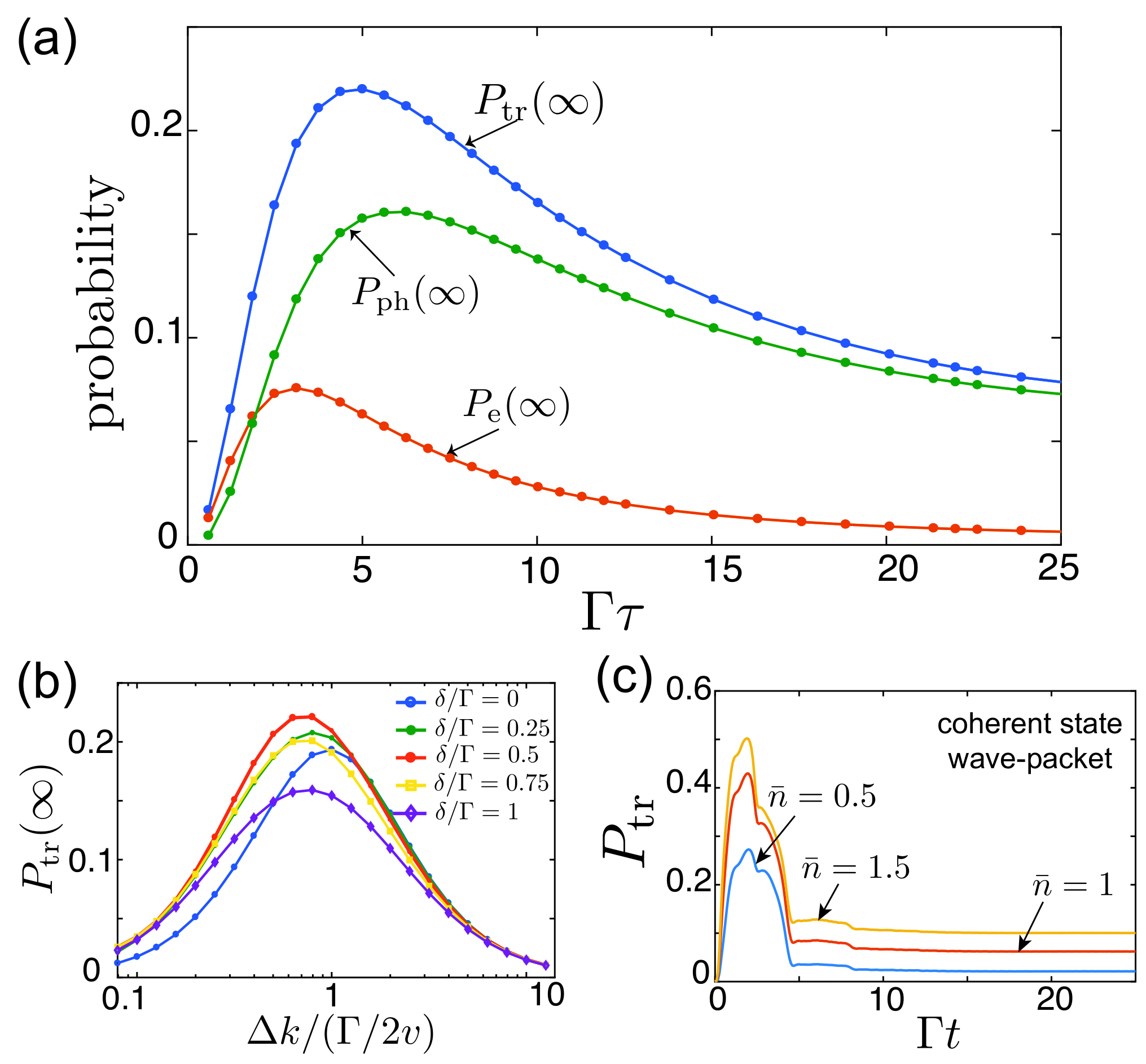
Dependence on time delay.—A substantial delay time is essential for exciting the BIC. The parameter set in Fig. 2, for instance, corresponds to . To highlight this dependence, we report in Fig. 3(a) the steady state values of , , and , optimized with respect to , as functions of . Both photon trapping and stationary qubit excitation are negligible in the Markovian regime , in sharp contrast to vacuum-decay schemes for which this is instead the optimal regime. A delay time is required to make our BIC generation scheme effective; indeed, each of the three probabilities reaches a maximum at a delay of order . Remarkably, becomes negligible compared to for , showing that the photon component is dominant at large delays as expected from Eqs. (2) and (3): In this regime, we thus get almost pure single-photon trapping
Dependence on bandwidth and detuning.—The efficiency of BIC generation depends on the width, , of the injected wavepacket. In Fig. 3(b) the optimal value is close to . Thus, photon absorption is maximum when the wavepacket width is of order the qubit decay rate, in agreement with general expectations Stobińska et al. 2009; Baragiola et al. 2012; Fang et al. 2018. The optimal as a function of delay time is given in the supplemental material Sup; for large , the optimal value saturates near .
Non-resonant photons can also be used to generate the BIC: results for a wavepacket of two photons detuned oppositely in energy are shown in Fig. 3(b). The optimal wavepacket width changes but remains of order . As the detuning increases, the maximum initially rises and then decays; note that the optimal detuning is . At this value the nonlinear scattering flux was shown to peak Fang and Baranger 2016; Fang and Baranger 2017, confirming that the intrinsic nonlinearity of the emitters is key to generating the BIC Sup.
Coherent-state wavepacket.—It is natural to wonder whether, instead of a two-photon pulse, the BIC can be excited using a coherent-state wavepacket, which is easier to generate experimentally. In Fig. 3(c) we consider the same setup, parameters, and wavepacket shape as in Fig. 2 but for a low-power coherent-state pulse Zheng et al. 2010 with the average photon number given by . For , is comparable to the one obtained with the two-photon pulse, demonstrating the effectiveness of using coherent states.
Increasing the BIC generation probability.—We find that the trapping probability depends sensitively on the shape of the incoming wavepacket. While we have mostly used (Figs. 2, 3, 5) the exponential pulse that is standard in the literature Fang et al. 2018; Rephaeli and Fan 2012, Fig. 4 shows how engineering the wavepacket shape strongly enhances Cotrufo and Alù 2018. We set here , which roughly corresponds to the maximum of in Fig. 3(a). The engineered incoming two-photon wavepacket in Fig. 4(a) (for methods see Sup) yields , a value about four times larger.
Two-qubit BIC.— A BIC very similar to the one addressed above occurs in an infinite waveguide (no mirror) coupled to a pair of identical qubits Ordonez et al. 2006; Tanaka et al. 2007; Gonzalez-Ballestero et al. 2013; Redchenko and Yudson 2014; Facchi et al. 2016; Facchi et al. 2018. With the qubits placed at and and for [Fig. 5(a)], there exists a BIC given by
| (9) |
where now , , and plus (minus) is used if is odd (even). By tracing out the photonic field, Eq. (9) clearly entails entanglement between the qubits. (In the familiar limit , for instance, the entangled state is , namely the sub- or super-radiant, maximally entangled state González-Tudela et al. 2011; Chang et al. 2012; Zheng and Baranger 2013; González-Tudela and Porras 2013; Lalumière et al. 2013; van Loo et al. 2013; Fang and Baranger 2015.) Thus, in the two-qubit setup of Fig. 5(a), our scattering-based approach to exciting the BIC can in particular generate entanglement.
This expectation is confirmed in Fig. 5(b), for which the same injected exponential wavepacket was used as in Fig. 2. In addition to the probability to excite at least one qubit and the probability to generate a BIC (9), we plot the amount of entanglement between the qubits, as measured by the concurrence Wootters 1998. As for one qubit, the two-qubit BIC population reaches a steady value after scattering, resulting in an excitation stored in the qubits and hence stationary entanglement. Note the typical Ficek and Tanaś 2008 “sudden birth” of the entanglement.
Conclusions.—We have shown that dressed BICs occurring in waveguide-QED setups can be generated via multi-photon scattering. This enables single-photon capture and, for multiple emitters, production of stationary entanglement. These BICs differ significantly from purely excitonic subradiant states, as well as from BICs located entirely within the side-coupled quantum system, in that they involve the field of the waveguide itself.
For our method, it is critical to have nonlinear emitters such as qubits; replacing them by bosonic modes, for example, will invalidate the whole scheme Sup.
While preparing this Letter we became aware of a related scheme by Cotrufo and Alù Cotrufo and Alù 2018. There however the BIC arises from a single system, comprised of a qubit and two cavities to provide feedback, side-coupled to an infinite waveguide. Here, instead, no cavities are present and the necessary quantum feedback is provided by a mirror [cf. Fig. 1] or the emitters themselves [cf. Fig. 5(a)]. Remarkably, in order to generate the BIC, this feedback needs to be delayed [cf. Fig. 3(a)].
Investigating the non-Markovian effects of non-negligible delays is a new frontier of quantum optics Tufarelli et al. 2013; Redchenko and Yudson 2014; Dorner and Zoller 2002; Carmele et al. 2013; Zheng and Baranger 2013; Tufarelli et al. 2014; Laakso and Pletyukhov 2014; Fang and Baranger 2015; Grimsmo 2015; Pichler and Zoller 2016; Ramos et al. 2016; Tabak and Mabuchi 2016; Whalen et al. 2017; Guimond et al. 2017; Pichler et al. 2017; Ritsch et al. 2013; Aspelmeyer et al. 2014; Wang and Safavi-Naeini 2017; Guo et al. 2017; Rossi et al. 2018; Chalabi and Waks 2018; Tabak et al. 2018; Chang et al. 2018; Torre and Illuminati 2018; Andersson et al. 2018; Fang et al. 2018. Here we have taken advantage of such delays, demonstrating that their role can be constructive Pichler et al. 2017; Torre and Illuminati 2018. In particular, within the range considered, as shown in Fig. 3(a), long delays () enable almost pure single-photon trapping (instead of hybrid atom-photon excitation). Remarkably, adding qubit losses, denoted by , makes the trapped photon decay slowly at the rate Sup, suggesting that our scheme is more robust against emitter loss for larger delay .
Targets of ongoing investigation include exploring the regime of very long delays (beyond in Fig. 3(a) allowed by our current computational capabilities Sup) and deriving a systematic criterion to increase the generation probability by wavepacket engineering (possibly by exploiting time reversal symmetry Stobińska et al. 2009; Cotrufo and Alù 2018). We expect this line of research will become important to, for example, long-distance communication over quantum networks.
We thank Peter Rabl, Shanhui Fan, and Tommaso Tufarelli for useful discussions. We acknowledge support from the U.S. DOE Office of Science Division of Materials Sciences and Engineering under Grant No. DE-SC0005237 and the Fulbright Research Scholar Program. The work at BNL was supported in part by BNL LDRD projects No. 17-029 and No. 19-002, and New York State Urban Development Corporation, d/b/a Empire State Development, under contract No. AA289. G. C. acknowledges support from the Austrian Science Fund (FWF) through SFB FOQUS F40, DK CoQuS W 1210, and the START grant Y 591-N16. Part of the computation was completed using resources of the Center for Functional Nanomaterials, which is a U.S. DOE Office of Science Facility, and the Scientific Data and Computing Center, a component of the Computational Science Initiative, at Brookhaven National Laboratory under Contract No. DE-SC0012704.
References
- Liao et al. (2016) Z. Liao, X. Zeng, H. Nha, and M. S. Zubairy, “Photon transport in a one-dimensional nanophotonic waveguide QED system,” Phys. Scr. 91, 063004 (2016).
- Roy et al. (2017) D. Roy, C. M. Wilson, and O. Firstenberg, “Colloquium: Strongly interacting photons in one-dimensional continuum,” Rev. Mod. Phys. 89, 021001 (2017).
- Gu et al. (2017) X. Gu, A. F. Kockum, A. Miranowicz, Y. X. Liu, and F. Nori, “Microwave photonics with superconducting quantum circuits,” Phys. Rep. 718, 1–102 (2017).
- Hsu et al. (2016) C. W. Hsu, B. Zhen, A. D. Stone, J. D. Joannopoulos, and M. Soljačić, “Bound states in the continuum,” Nat. Rev. Mater. 1, 16048 (2016).
- Kimble (2008) H. J. Kimble, “The quantum internet,” Nature 453, 1023 (2008).
- Lvovsky et al. (2009) A. I. Lvovsky, B. C. Sanders, and W. Tittel, “Optical quantum memory,” Nat. Photonics 3, 706 (2009).
- Saglamyurek et al. (2018) E. Saglamyurek, T. Hrushevskyi, A. Rastogi, K. Heshami, and L. J. LeBlanc, “Coherent storage and manipulation of broadband photons via dynamically controlled Autler–Townes splitting,” Nat. Photonics (2018).
- Ordonez et al. (2006) G. Ordonez, K. Na, and S. Kim, “Bound states in the continuum in quantum-dot pairs,” Phys. Rev. A 73, 022113 (2006).
- Longhi (2007) S. Longhi, “Bound states in the continuum in a single-level Fano-Anderson model,” Eur. Phys. J. B 57, 45–51 (2007).
- Tanaka et al. (2007) S. Tanaka, S. Garmon, G. Ordonez, and T. Petrosky, “Electron trapping in a one-dimensional semiconductor quantum wire with multiple impurities,” Phys. Rev. B 76, 153308 (2007).
- Tufarelli et al. (2013) T. Tufarelli, F. Ciccarello, and M. S. Kim, “Dynamics of spontaneous emission in a single-end photonic waveguide,” Phys. Rev. A 87, 013820 (2013).
- Gonzalez-Ballestero et al. (2013) C. Gonzalez-Ballestero, F. J. Garcia-Vidal, and E. Moreno, “Non-Markovian effects in waveguide-mediated entanglement,” New J. Phys. 15, 073015 (2013).
- Redchenko and Yudson (2014) E. S. Redchenko and V. I. Yudson, “Decay of metastable excited states of two qubits in a waveguide,” Phys. Rev. A 90, 063829 (2014).
- Facchi et al. (2016) P. Facchi, M. S. Kim, S. Pascazio, F. V. Pepe, D. Pomarico, and T. Tufarelli, “Bound states and entanglement generation in waveguide quantum electrodynamics,” Phys. Rev. A 94, 043839 (2016).
- Facchi et al. (2018) P. Facchi, S. Pascazio, F. V. Pepe, and K. Yuasa, “Long-lived entanglement of two multilevel atoms in a waveguide,” J. Phys. Commun. 2, 035006 (2018).
- Shen and Fan (2005) J. T. Shen and S. Fan, “Coherent single photon transport in a one-dimensional waveguide coupled with superconducting quantum bits,” Phys. Rev. Lett. 95, 213001 (2005).
- Chang et al. (2007) D. E. Chang, A. S. Sørensen, E. A. Demler, and M. D. Lukin, “A single-photon transistor using nanoscale surface plasmons,” Nature Phys. 3, 807–812 (2007).
- González-Tudela et al. (2011) A. González-Tudela, D. Martin-Cano, E. Moreno, L. Martín-Moreno, and F. Tejedor, C./García-Vidal, “Entanglement of two qubits mediated by one-dimensional plasmonic waveguides,” Phys. Rev. Lett. 106, 020501 (2011).
- González-Tudela and Porras (2013) A. González-Tudela and D. Porras, “Mesoscopic entanglement induced by spontaneous emission in solid-state quantum optics,” Phys. Rev. Lett. 110, 080502 (2013).
- Chang et al. (2012) D. E. Chang, L. Jiang, A. V. Gorshkov, and H. J. Kimble, “Cavity QED with atomic mirrors,” New J. Phys. 14, 063003 (2012).
- Longo et al. (2010) P. Longo, P. Schmitteckert, and K. Busch, “Few-photon transport in low-dimensional systems: Interaction-induced radiation trapping,” Phys. Rev. Lett. 104, 023602 (2010).
- Longo et al. (2011) P. Longo, P. Schmitteckert, and K. Busch, “Few-photon transport in low-dimensional systems,” Phys. Rev. A 83, 063828 (2011).
- Lombardo et al. (2014) F. Lombardo, F. Ciccarello, and G. M. Palma, “Photon localization versus population trapping in a coupled-cavity array,” Phys. Rev. A 89, 053826 (2014).
- Calajó et al. (2016) G. Calajó, F. Ciccarello, D. E. Chang, and P. Rabl, “Atom-field dressed states in slow-light waveguide QED,” Phys. Rev. A 93, 033833 (2016).
- Shi et al. (2016) T. Shi, Y.-H. Wu, A. González-Tudela, and J. I. Cirac, “Bound states in boson impurity models,” Phys. Rev. X 6, 021027 (2016).
- Kocabaş (2016) Ş. E. Kocabaş, “Effects of modal dispersion on few-photon–qubit scattering in one-dimensional waveguides,” Phys. Rev. A 93, 033829 (2016).
- Shukla and Eliasson (2011) P. K. Shukla and B. Eliasson, “Colloquium: Nonlinear collective interactions in quantum plasmas with degenerate electron fluids,” Rev. Mod. Phys. 83, 885–906 (2011).
- García-Mata et al. (2014) I. García-Mata, C. Pineda, and D. A. Wisniacki, “Quantum non-Markovian behavior at the chaos border,” J. Phys. A 47, 115301 (2014).
- Swingle (2018) B. Swingle, “Unscrambling the physics of out-of-time-order correlators,” Nat. Phys. 14, 988–990 (2018).
- Ritsch et al. (2013) H. Ritsch, P. Domokos, F. Brennecke, and T. Esslinger, “Cold atoms in cavity-generated dynamical optical potentials,” Rev. Mod. Phys. 85, 553–601 (2013).
- Aspelmeyer et al. (2014) M. Aspelmeyer, T. J. Kippenberg, and F. Marquardt, “Cavity optomechanics,” Rev. Mod. Phys. 86, 1391–1452 (2014).
- Wang and Safavi-Naeini (2017) Z. Wang and A. H. Safavi-Naeini, “Enhancing a slow and weak optomechanical nonlinearity with delayed quantum feedback,” Nat. Commun. 8, 15886 (2017).
- Rossi et al. (2018) M. Rossi, N. Kralj, S. Zippilli, R. Natali, A. Borrielli, G. Pandraud, E. Serra, G. Di Giuseppe, and D. Vitali, “Normal-mode splitting in a weakly coupled optomechanical system,” Phys. Rev. Lett. 120, 073601 (2018).
- Shen and Fan (2007) J.-T. Shen and S. Fan, “Strongly correlated multiparticle transport in one dimension through a quantum impurity,” Phys. Rev. A 76, 062709 (2007).
- Shen and Fan (2009) J.-T. Shen and S. Fan, “Theory of single-photon transport in a single-mode waveguide,” Phys. Rev. A 79, 023837 (2009).
- Zheng et al. (2010) H. Zheng, D. J. Gauthier, and H. U. Baranger, “Waveguide QED: Many-body bound-state effects in coherent and Fock-state scattering from a two-level system,” Phys. Rev. A 82, 063816 (2010).
- Zheng and Baranger (2013) H. Zheng and H. U. Baranger, “Persistent quantum beats and long-distance entanglement from waveguide-mediated interactions,” Phys. Rev. Lett. 110, 113601 (2013).
- (38) Here the plus sign occurs for even, while the minus sign is for odd.
- Tufarelli et al. (2014) T. Tufarelli, M. S. Kim, and F. Ciccarello, “Non-Markovianity of a quantum emitter in front of a mirror,” Phys. Rev. A 90, 012113 (2014).
- Hoi et al. (2015) I.-C. Hoi, A. F. Kockum, L. Tornberg, A. Pourkabirian, G. Johansson, P. Delsing, and C. M. Wilson, “Probing the quantum vacuum with an artificial atom in front of a mirror,” Nat. Phys. 11, 1045–1049 (2015).
- (41) See Supplementary Material at [URL] for computational methods used in this work (see also Ref. Fang 2019), derivation of Eq. (8), optimal used in Fig. 3(a), explanation of the method used to increase BIC generation probability in Fig. 4, additional notes on the two-qubit BIC, impact of nonzero loss to photon trapping, and the importance of having nonlinear emitters.
- Stobińska et al. (2009) M. Stobińska, G. Alber, and G. Leuchs, “Perfect excitation of a matter qubit by a single photon in free space,” Eur.ophys. Lett. 86, 14007 (2009).
- Baragiola et al. (2012) B. Q. Baragiola, R. L. Cook, A. M. Brańczyk, and J. Combes, “N-photon wave packets interacting with an arbitrary quantum system,” Phys. Rev. A 86, 013811 (2012).
- Fang et al. (2018) Y.-L. L. Fang, F. Ciccarello, and H. U. Baranger, “Non-Markovian dynamics of a qubit due to single-photon scattering in a waveguide,” New J. Phys. 20, 043035 (2018).
- Fang and Baranger (2016) Y.-L. L. Fang and H. Baranger, “Photon correlations generated by inelastic scattering in a one-dimensional waveguide coupled to three-level systems,” Physica 78E, 92–99 (2016).
- Fang and Baranger (2017) Y.-L. L. Fang and H. U. Baranger, “Multiple emitters in a waveguide: Nonreciprocity and correlated photons at perfect elastic transmission,” Phys. Rev. A 96, 013842 (2017).
- Rephaeli and Fan (2012) E. Rephaeli and S. Fan, “Stimulated emission from a single excited atom in a waveguide,” Phys. Rev. Lett. 108, 143602 (2012).
- Cotrufo and Alù (2018) M. Cotrufo and A. Alù, “Single-photon embedded eigenstates in coupled cavity-atom systems,” (2018), arXiv:1805.03287 .
- Lalumière et al. (2013) K. Lalumière, B. C. Sanders, A. F. van Loo, A. Fedorov, A. Wallraff, and A. Blais, “Input-output theory for waveguide QED with an ensemble of inhomogeneous atoms,” Phys. Rev. A 88, 043806 (2013).
- van Loo et al. (2013) A. F. van Loo, A. Fedorov, K. Lalumière, B. C. Sanders, A. Blais, and A. Wallraff, “Photon-Mediated Interactions Between Distant Artificial Atoms,” Science 342, 1494–1496 (2013).
- Fang and Baranger (2015) Y.-L. L. Fang and H. U. Baranger, “Waveguide QED: Power spectra and correlations of two photons scattered off multiple distant qubits and a mirror,” Phys. Rev. A 91, 053845 (2015), ibid. 96, 059904(E) (2017).
- Wootters (1998) W. K. Wootters, “Entanglement of formation of an arbitrary state of two qubits,” Phys. Rev. Lett. 80, 2245–2248 (1998).
- Ficek and Tanaś (2008) Z. Ficek and R. Tanaś, “Delayed sudden birth of entanglement,” Phys. Rev. A 77, 054301 (2008).
- Dorner and Zoller (2002) U. Dorner and P. Zoller, “Laser-driven atoms in half-cavities,” Phys. Rev. A 66, 023816 (2002).
- Carmele et al. (2013) A. Carmele, J. Kabuss, F. Schulze, S. Reitzenstein, and A. Knorr, “Single Photon Delayed Feedback: A Way to Stabilize Intrinsic Quantum Cavity Electrodynamics,” Phys. Rev. Lett. 110, 013601 (2013).
- Laakso and Pletyukhov (2014) M. Laakso and M. Pletyukhov, “Scattering of two photons from two distant qubits: Exact solution,” Phys. Rev. Lett. 113, 183601 (2014).
- Grimsmo (2015) A. L. Grimsmo, “Time-Delayed Quantum Feedback Control,” Phys. Rev. Lett. 115, 060402 (2015).
- Pichler and Zoller (2016) H. Pichler and P. Zoller, “Photonic Circuits with Time Delays and Quantum Feedback,” Phys. Rev. Lett. 116, 093601 (2016).
- Ramos et al. (2016) T. Ramos, B. Vermersch, P. Hauke, H. Pichler, and P. Zoller, “Non-Markovian dynamics in chiral quantum networks with spins and photons,” Phys. Rev. A 93, 062104 (2016).
- Tabak and Mabuchi (2016) G. Tabak and H. Mabuchi, “Trapped modes in linear quantum stochastic networks with delays,” EPJ Quantum Technol. 3, 3 (2016).
- Whalen et al. (2017) S. J. Whalen, A. L. Grimsmo, and H. J. Carmichael, “Open quantum systems with delayed coherent feedback,” Quantum Science and Technology 2, 044008 (2017).
- Guimond et al. (2017) P.-O. Guimond, M. Pletyukhov, H. Pichler, and P. Zoller, “Delayed coherent quantum feedback from a scattering theory and a matrix product state perspective,” Quantum Sci. Technol. 2, 044012 (2017).
- Pichler et al. (2017) H. Pichler, S. Choi, P. Zoller, and M. D. Lukin, “Universal photonic quantum computation via time-delayed feedback,” Proc. Natl. Acad. Sci. 114, 11362–11367 (2017).
- Guo et al. (2017) L. Guo, A. Grimsmo, A. F. Kockum, M. Pletyukhov, and G. Johansson, “Giant acoustic atom: A single quantum system with a deterministic time delay,” Phys. Rev. A 95, 053821 (2017).
- Chalabi and Waks (2018) H. Chalabi and E. Waks, “Interaction of photons with a coupled atom-cavity system through a bidirectional time-delayed feedback,” Phys. Rev. A 98, 063832 (2018).
- Tabak et al. (2018) G. Tabak, R. Hamerly, and H. Mabuchi, “Factorization of linear quantum systems with delayed feedback,” (2018), arXiv:1803.01539 .
- Chang et al. (2018) C.-Y. Chang, L. Lanco, P. Senellart, and D. S. Citrin, “Quantum stabilization of a single-photon emitter in a coupled microcavity–half-cavity system,” (2018), arXiv:1804.06734 .
- Torre and Illuminati (2018) G. Torre and F. Illuminati, “Non-Markovianity-assisted optimal continuous variable quantum teleportation,” (2018), arXiv:1805.03617 .
- Andersson et al. (2018) G. Andersson, B. Suri, L. Guo, T. Aref, and P. Delsing, “Nonexponential decay of a giant artificial atom,” (2018), arXiv:1812.01302 .
- Fang (2019) Y.-L. L. Fang, “FDTD: Solving 1+1D delay PDE in parallel,” Comput. Phys. Commun. 235, 422 – 432 (2019).
bsmi
Supplementary Material for “Exciting a Bound State in the Continuum through Multiphoton Scattering Plus Delayed Quantum Feedback”
Giuseppe Calajó Present address: ICFO-Institut de Ciencies Fotoniques, 08860 Castelldefels (Barcelona), Spain. Contact email giuseppe.calajo@icfo.eu.
Yao-Lung L. Fang (方耀龍) Present address Present address
Harold U. Baranger
Francesco Ciccarello
January 13, 2019
S1 Computational methods
In order to solve for various wavefunctions in the waveguide-QED setups that we consider, we have taken two different routes: treating the 1D field as a continuum or discretizing it as an effective coupled-cavity array (CCA) and working in the middle of the band, where band-edge effects are minimized and the dispersion is close to linear. In the main text, results shown in Figs. 2 and 3(a)-(b) were obtained through the continuum approach, while the discrete approach was employed for producing Figs. 3(c), 4 and 5.
S1.1 Continuum approach
For the continuum case, we follow the approach reported in Ref. Fang et al. 2018: Starting from the Schrödinger equation, by unfolding the half space and tracing out the two-photon part, we arrive at a (1+1)-dimensional delay partial differential equation for the wavefunction [joint amplitude for qubit and one photon at position , c.f. Eq. (5) of the main text], which we solve using a tailored finite-difference time-domain (FDTD) code that has multithreading support for reducing the computation time considerably Fang 2019.11 1 This FDTD code is open-sourced at https://github.com/leofang/FDTD and also available in Ref. Fang 2019. The two-photon wavefunction can be constructed straightforwardly once is solved Fang et al. 2018; Fang 2019. Our FDTD code provides the numerically exact solution to the dynamics in the two-excitation sector.
For solving the two-photon scattering problem of interest, we send in a two-photon exponential wavepacket with the qubit initially unexcited (set init_cond=3 in the code). In the region , the exact solution to is given by
| (S1) |
where is the qubit wavefunction in the one-excitation sector, solved by assuming the qubit is initially unexcited and the presence of an incident single-photon wavepacket , and is the normalization constant for the two-photon wavepacket (see the main text). With this expression, the problem of computing for becomes well-defined and is solved by FDTD Fang 2019.
Our FDTD code is mainly memory bound. For typical cases (such as Fig. 2) we need at least 128 GB of RAM. For the most extreme case that we explored [ in Fig. 3(a), corresponding to with ], we use a machine with 450+ GB of RAM in the local cluster. A rule of thumb for estimating the memory usage is to take (in GB), where is the number of FDTD steps for completing a round trip between the atom and the mirror; all input parameters are explained in detail in Fang 2019. In the aforementioned most demanding case, both and are about and (such that one resonant wavelength has + FDTD steps, yielding an accuracy of order ), so the -array alone takes roughly 438 GB. Useful tricks to explore the large regime include reducing [since ] and reducing . For these reasons we set for the plots in Fig. 2 and Fig. 3(b) and for the plot in Fig. 3(a), where, as previously mentioned, we explored the regime of long delay time. In this way, with the same amount of memory, we were able to complete more FDTD steps at the expense of reduced accuracy (obviously careful checks were necessary). Note that the larger the longer the cutoff time needs to be because of the multiple bounces of the photon field before escaping.
S1.2 Discrete approach
An alternative approach to simulate the two-photon scattering process consists in modeling it as a CCA comprised of a 1D arrangement of identical resonators of frequency with nearest-neighbour coupling rate , with one resonator coupled to the qubit with coupling rate . Hamiltonian (1) of the main text is thus discretized as
| (S2) |
where () annihilates (creates) a photon on the th cavity mode while and (here stands for the longitudinal size of each fictitious cavity). By introducing the momentum operators , with (we are implicitly rescaling the wavevector as ), the first two terms of Eq. (S2), which represent the free field Hamiltonian , can be arranged in the diagonal form , with the normal frequencies
| (S3) |
forming a band of width centered at the bare cavity frequency . The dispersion law (S3) is approximately linear for . Thus, in the weak-coupling regime and for , Hamiltonian (S2) is a reasonable approximation to the physics of the continuous-waveguide Hamiltonian (1) of the main text. The advantage of using this discrete model is that it can be easily handled numerically up to the third-excitation sector of the Hilbert space. In particular, in this work we simulate the time-dependent Schrödinger equation corresponding to Eq. (S2) for () cavities for the two-(three-) excitation subspace and set in order to be consistent with the weak-coupling assumption. In particular we have used for Figs. 3(c) and 5 and for Fig. 4.
It is worth mentioning that, in the present finite-band CCA, even bound states outside the band can occur Calajó et al. 2016 (in Ref. Longo et al. 2010 it was shown that they can be populated via two-photon scattering). However, the assumption () ensures that the BIC lies exactly at the center of the band in a way that processes that excite the bound states outside the continuum are energetically forbidden (see Calajó et al. 2016).
Finally, note that the present discrete approach is straightforwardly extended to describe the two-qubit setup in Fig. 5 of the main text. In this case, we place the two emitters far from the CCA edges to avoid unwanted back-reflection from the array’s ends within the considered simulation time.
S2 Derivation of Eq. (8)
The BIC state has the structure (see main text)
| (S4) |
where
| (S5) |
Based on definitions (5) and (6) of the main text, we thus find that in the case of state (7)
| (S6) |
where it is understood that time is large enough that the scattering is complete. Hence, due to the normalization condition in Eqs. (S5),
| (S7) |
Next, combining the last identity in (S5) with the first of Eqs. (S6) yields . Thereby,
| (S8) |
which completes the proof of Eq. (8) in the main text.
S3 Optimal width for resonant two-photon wavepackets
In Fig. 3(a) of the main text, we plot various probabilities against , each obtained after an optimization over the wavepacket width . In Fig. S1, we plot the optimal , denoted by , as a function of . We find that, for delays such that , scales approximately as . For larger delays, instead saturates to a non-zero value (presumably in order to maximize the atomic absorption during the scattering transient). For each set value of , the optimization was carried out by interpolating the ’s data computed on a discrete -grid (on a log scale) and working out the at which the curve exhibits a local maximum.

S4 Increasing the BIC generation probability
Fig. 4 of the main text reports a paradigmatic example showing that can be strongly increased (compared to the standard choice of an exponential pulse) by engineering the wavepacket shape. Here, we describe how the wavepacket in Fig. 4 was derived.
The BIC generation process would be perfect () if, in Eq. (7) of the main text, , meaning that the incoming two-photon wavepacket deterministically evolves at the end of scattering into the BIC plus a (normalized) outgoing single-photon wavepacket . The basic idea is to consider the time-reversed version of such ideal process: the system is initially prepared in the dressed BIC and an incoming single-photon wavepacket undergoes scattering resulting in a normalized outgoing two-photon wavepacket at the end of scattering Cotrufo and Alù 2018. If such a single-photon wavepacket exists, then sending on the initially unexcited qubit the time-reversed version of will deterministically yield the BIC (plus an outgoing photon).
Based on the above, we considered a right-incoming, Gaussian, single-photon wavepacket of the form
| (S9) |
where is the spatial width and , which is injected toward the qubit-mirror region initially prepared in the BIC [see Fig. S2(a)]. At the end of scattering, as shown in Fig. S2(b), part of the excitation trapped in the BIC is released, while a residual amount remains. Minimizing the latter over the width yields . The final joint state is of the same form as Eq. (7) in the main text, featuring in particular an outgoing two-photon component. We normalize and time-reverse this two-photon wavefunction, which is then used as the input of our original problem (namely, it is sent to the scattering region with the qubit initially in the ground state) as shown in Fig. S2(c). It turns out [see Fig. S2(d)] that the resulting two-photon-wavepacket is far more effective than the exponential one (see Figs. 2 and 3 in the main text), leading to the BIC generation probability .
A further improvement can be obtained by repeating the above process, but this time choosing as the single-photon outgoing component of Fig. S2(c) (once this is normalized and time-reversed). One more iteration of this procedure yields the results in Fig. 5 of the main text, where we obtain in particular (further iterations do not substantially change this value).
In this paradigmatic instance, we started from a Gaussian-shaped single-photon wavepacket. Deriving a systematic, general optimization criterion that does not rely on such a specific choice is the target ongoing investigation, in particular with the goal to assess whether the BIC generation probability can approach 100%.
S5 Two-qubit BIC
In Fig. 5(b) of the main text we plot , and the concurrence for the two-qubit setup of Fig. 5(a). Here, we provide detailed definitions of these quantities.
As in the case of a qubit in front of a mirror [cf. Eq. (5) in the main text], the joint state at time lives in the two-excitation sector and thus has the general form
| (S10) |
Accordingly, the total probability that at least one qubit is excited reads
| (S11) |
while the probability that one photon lies between the two qubits and one beyond them is given by
| (S12) |
while their sum is called .
To measure the amount of qubit-qubit entanglement in state (S10), we trace out the field degrees of freedom to get the reduced two-qubit density matrix and next calculate the corresponding Wootters concurrence Wootters 1998. This takes the form
| (S13) |
where
| (S14) |
are the atomic coherences.
S6 Resilience to qubit losses into an external reservoir
In the main text, we considered ideal setups in which each qubit is perfectly coupled to the waveguide. In practice, the emitters may be also in contact with modes other than the waveguide, which introduces additional decay channels. Assuming a Markovian external reservoir and given our purpose of describing a scattering process, such dissipation can be accounted for by adding to the Hamiltonian Eq. (1) of the main text an effective non-Hermitian term Shen and Fan 2007; Zheng et al. 2010 (we consider the setup of Fig. 1 in the main text):
| (S15) |
where is the decay rate of the qubit into the external environment.
In Fig. S3, we use the same parameters as in Fig. 2 of the main text and study how the time dependence of is affected by the loss rate (recall that for the asymptotic value of is the probability of generating the BIC, ). In the range considered ( up to 10% of , the decay rate into the waveguide modes) the presence of a nonzero loss indeed turns the long-time saturation at into a slow decay. We found strong numerical evidence that the long-time behavior of is described by the function with for [see Eqs. (8), (S7) and (S8)] and being the emitter’s population in the BIC [see Eqs. (3) and (4) in the main text]. This finding can be heuristically explained through the following simple argument. The non-Hermitian term in Eq. (S15) can be equivalently expressed as , where we set . The effective representation of this in the (one-dimensional) BIC subspace is obtained upon projection as
| (S16) |
indicating that for the BIC decays at rate .
It follows that the smaller the excitonic fraction , the more robust is the BIC to emitter losses. Since decreases with [cf. Eq. (3) in the main text] it turns out that the longer the delay, the more resilient is the BIC generation scheme to loss. This thus embodies a further significant advantage compared to generation schemes based on spontaneous emission (see discussion in the main text), especially if one aims at an almost pure single-photon trapping.
A detailed discussion of the effect of qubit losses on single-photon BICs, which explicitly takes into account the degrees of freedom of the extra reservoir, is presented in Ref. Gonzalez-Ballestero et al. 2013 (in particular it is shown that the external bath dresses the BIC and scattering states without affecting their orthogonality).
S7 Role of emitter nonlinearity in the BIC generation scheme
In the main text, we stressed that the qubit nonlinearity is key to generate the BIC. In this section, we further illustrate this point in terms of a bosonic Hamiltonian that depends in particular on the strength of nonlinearity Longo et al. 2010; Fang and Baranger 2015. For the sake of argument, we focus again on the one-qubit setup of Fig. 1.
Consider the bosonic Hamiltonian
| (S17) |
Here, is in the same form as in Eq. (1) of the main text except for the replacement , where and fulfill bosonic commutation relations and commute with all the waveguide operators. The quartic term describes a fictitious, on-site boson-boson repulsion at the emitter’s location. When this is absent, i.e. for , Eq. (S17) is equivalent to replacing the qubit with a bosonic mode, which makes the total Hamiltonian fully bosonic and quadratic. For , the effect of is to make energetically unfavorable the occupation of emitter’s number states with so that in the limit of infinite this behaves as an effective qubit and we recover the Hamiltonian Eq. (1):
| (S18) |
We next discuss the cases and separately.
S7.1
In this case, the Hamiltonian is bosonic and quadratic and can thereby be diagonalized straightforwardly in terms of the normal modes. In the single-excitation sector , where , the eigenstates of (S17) consist of scattering states and a bound state such that and , respectively. The corresponding wavefunctions are given by , where and the normal-mode operators are defined as
| (S19) |
with . Here, the amplitudes and are the same as those defining the corresponding single-excitation stationary states of the one-qubit Hamiltonian . Regardless of , normal-mode operators allow one to express the Hamiltonian in the diagonal form
| (S20) |
In the two-excitation sector, corresponding to , the eigenstates read
| (S21) |
with eigenvalues , and , respectively. These are physically interpreted as follows:
- -
states are two-photon scattering states describing two incoming photons that scatter off the emitter and mirror and are eventually fully reflected;
- -
states are semi-bound states: one photon scatters off while another photon is confined between the emitter and mirror dressing the emitter so as to form the single-excitation bound state ;
- -
state is a two-photon bound state, featuring in particular two photons fully confined within the mirror-emitter interspace.
Based on these, we see that the scheme for generating the BIC via two-photon scattering becomes fully ineffective when the qubit is replaced by a bosonic mode: injecting two photons with the emitter initially unexcited involves only the stationary states , which have no overlap with other eigenstates and . The emitter will typically be excited during the scattering transient, but the two photons will be eventually fully reflected with no light confined in the mirror-emitter interspace. This conclusion holds regardless of the parameters, hence in particular no matter how long the time delay.
S7.2
The last conclusion does not hold any more when the fictitious bosonic repulsive term is present [cf. Eq. (S17)]. In the two-excitation sector , this takes the effective form with . Noting now that in the same subspace all the stationary states [see Eq. (S21)] generally feature a term we see that the repulsive interaction mixes together all the eigenstates of . Most importantly, this means that introducing the nonlinearity has in particular the effects of (i) connecting two-photon scattering states to semi-bound ones [see Eq. (S21)] and (ii) eliminating, as , the two-photon bound state .
Indeed, using the Lippmann-Schwinger formalism, it can be shown that the unbound stationary states of have the following form Fang and Baranger 2015
| (S22) |
where with , is the retarded Green’s function for , and . Overlaps between the eigenstate and other states can be easily computed by noting that all matrix elements can be expressed in terms of the amplitudes and from the single-excitation sector Fang and Baranger 2015. In the limit of , Eq. (S22) becomes
| (S23) |
which in particular entails . Thus, it is clearly impossible to doubly occupy the emitter, and the 2LS behavior is correctly recovered.
This argument provides further physical intuition as to why the nonlinearity of the 2LS, in this picture encoded in the repulsive term , is essential for the BIC generation scheme via two-photon scattering. In particular, it shows how the intrinsic qubit nonlinearity enables the process where two incoming photons can evolve with some probability into a single scattering photon and the single-photon bound state .
To further support the above conclusion, using the method of Sec. S1.2 we numerically computed in a paradigmatic case the asymptotic trapping probability for the bosonic Hamiltonian (S17) as a function of the nonlinearity parameter . The definition of is formally analogous to the one where the emitter is a qubit except that the probability of finding the emitter doubly excited (population of state ) is now also included. As shown in Fig. S4, vanishes when (bosonic emitter) and then overall grows with , eventually converging as to the corresponding value obtained with a qubit.

As a final remark, we mention that, while for multi-photon BICs do exist and are simply given by , for the two-level emitter addressed in the main text (corresponding to ) in the range of parameters considered in this work we did not find any numerical evidence of their existence, which can be checked simply by examining the conservation of probability.
References
- Fang et al. (2018) Y.-L. L. Fang, F. Ciccarello, and H. U. Baranger, “Non-Markovian dynamics of a qubit due to single-photon scattering in a waveguide,” New J. Phys. 20, 043035 (2018).
- Fang (2019) Y.-L. L. Fang, “FDTD: Solving 1+1D delay PDE in parallel,” Comput. Phys. Commun. 235, 422 – 432 (2019).
- Calajó et al. (2016) G. Calajó, F. Ciccarello, D. E. Chang, and P. Rabl, “Atom-field dressed states in slow-light waveguide QED,” Phys. Rev. A 93, 033833 (2016).
- Longo et al. (2010) P. Longo, P. Schmitteckert, and K. Busch, “Few-photon transport in low-dimensional systems: Interaction-induced radiation trapping,” Phys. Rev. Lett. 104, 023602 (2010).
- Cotrufo and Alù (2018) M. Cotrufo and A. Alù, “Single-photon embedded eigenstates in coupled cavity-atom systems,” (2018), arXiv:1805.03287 .
- Wootters (1998) W. K. Wootters, “Entanglement of formation of an arbitrary state of two qubits,” Phys. Rev. Lett. 80, 2245–2248 (1998).
- Shen and Fan (2007) J.-T. Shen and S. Fan, “Strongly correlated multiparticle transport in one dimension through a quantum impurity,” Phys. Rev. A 76, 062709 (2007).
- Zheng et al. (2010) H. Zheng, D. J. Gauthier, and H. U. Baranger, “Waveguide QED: Many-body bound-state effects in coherent and Fock-state scattering from a two-level system,” Phys. Rev. A 82, 063816 (2010).
- Gonzalez-Ballestero et al. (2013) C. Gonzalez-Ballestero, F. J. Garcia-Vidal, and E. Moreno, “Non-Markovian effects in waveguide-mediated entanglement,” New J. Phys. 15, 073015 (2013).
- Fang and Baranger (2015) Y.-L. L. Fang and H. U. Baranger, “Waveguide QED: Power spectra and correlations of two photons scattered off multiple distant qubits and a mirror,” Phys. Rev. A 91, 053845 (2015), ibid. 96, 059904(E) (2017).
2, apsrev41Controlapsrev41Control