Chaotic Synchronization between Atomic Clocks
Abstract
We predict synchronization of the chaotic dynamics of two atomic ensembles coupled to a heavily damped optical cavity mode. The atoms are dissipated collectively through this mode and pumped incoherently to achieve a macroscopic population of the cavity photons. Even though the dynamics of each ensemble are chaotic, their motions repeat one another. In our system, chaos first emerges via quasiperiodicity and then synchronizes. We identify the signatures of synchronized chaos, chaos, and quasiperiodicity in the experimentally observable power spectra of the light emitted by the cavity.
I Introduction
It is generally challenging to predict the long term behavior of a chaotic system, e.g., weather, due to its sensitive dependence on initial conditions. However, there are special chaotic systems where the dynamics of one part are locked or synchronized with those of the other part or parts Uchida; Chaotic_Synch_1. As a result, the asymptotic behavior of certain dynamical variables is fully predictable in spite of the overall chaotic nature. Different mechanisms of obtaining chaotic synchronization have been studied in, for example, electrical circuits Chaotic_Synch_2; Chaotic_Synch_3, coupled lasers Chaotic_Synch_4; Chaotic_Synch_5; Chaotic_Synch_6, oscillators in laboratory plasma Chaotic_Synch_7, population dynamics Chaotic_Synch_8 and earthquake models Chaotic_Synch_9. In this paper, we report chaotic synchronization in a novel physical system, namely, between two mutually coupled ensembles of atoms in a driven-dissipative experimental setup. This is unlike most other examples of chaotic synchronization, where the coupling between the two parts is unidirectional. In the chaotic synchronized phase, our system has potential applications in secure communication Uchida; Chaotic_Synch_1; Chaotic_Synch_2; Chaotic_Synch_3; Chaotic_Synch_6.


We consider two spatially separated ensembles of, e.g., atoms inside a bad (leaky) optical cavity, see Fig. 1. The atoms are collectively dissipated through a Rabi coupling to a heavily damped cavity mode and pumped with a transverse laser to achieve a macroscopic population of the cavity photons Holland_Two_Ensemble_Expt. A single atomic ensemble coupled to a bad cavity has been proposed as a source of ultracoherent radiation for an atomic clock Holland_atomic_clock. The two ensembles in our setup, therefore, represent two interacting atomic clocks Holland_Two_Ensemble_Theory. Previous work obtained main nonequilibrium phases of this system Holland_Two_Ensemble_Theory; Patra_1, see the inset in Fig. 2.
In this paper, we study a finite region of the phase diagram – the orange (nonsynchronized chaos) and red (synchronized chaos) points in region III of Fig. 2 – where the light radiated by the cavity behaves chaotically. Here chaos appears via quasiperiodicity Hilborn; QP_Chaos_1; QP_Chaos_2. Initially, chaotic trajectories fill up extended regions in the configuration space, see Fig. 3e. We discover a subregion inside the chaotic phase where dynamics are confined to a flat hypersurface (Fig. 3h), called the “synchronization manifold”. Essentially, the time dependence of one ensemble follows that of the other. We also study signatures of these novel behaviors in the power spectra of the radiated light. Unlike the quasiperiodic power spectrum (Fig. 3c), which consists of discrete peaks, the chaotic one (Fig. 3f) is a continuum. The chaotic synchronized spectrum (Fig. 3i) additionally has a reflection symmetry about zero and no peak at zero frequency, see the insets in Figs. 3f and 3i.
II Nonchaotic Phases
We model our system (cf. Fig. 1) with the following master equation for the density matrix :
| (1a) | |||||
| (1b) | |||||
The Hamiltonian describes two atomic ensembles A and B Rabi coupled (with frequency ) to the cavity mode , where create (annihilate) cavity photons. Each ensemble contains a large number of atoms, e.g., of atoms Holland_Two_Ensemble_Theory; Holland_Two_Ensemble_Expt. We focus on the lasing transition between two atomic levels. Consequently, we describe individual atoms with Pauli matrices and the atomic ensembles with collective spin operators and . Experimentally, the level-spacings are controlled with two distinct Raman dressing lasers Holland_Two_Ensemble_Expt. We model the energy nonconserving processes (decay of the bad cavity mode with a rate , and incoherent pumping by external lasers at an effective repump rate ) by Lindblad superoperators,
| (2) |
Using the adiabatic approximation Bad_cavity, which is exact in the limit , we eliminate the cavity mode replacing . Finally, in the rotating frame, where frequencies are shifted by the mean level-spacing (it is equal to the clock transition frequency, which is GHz for ), we derive semiclassical evolution equations using the mean-field approximation, ,
| (3a) | |||||
| (3b) | |||||
where , , , is the total classical spin, and . In Eq. (3) and from now on, we express the detuning and the repump rate in the units of the collective decay rate ( kHz for a typical experimental setup Holland_Two_Ensemble_Expt) and replace .
The mean-field equations of motion possess two symmetries: Axial symmetry , where is a rotation by an angle around the -axis. Indeed, the replacement leaves Eq. (3) unchanged. symmetry which involves a rotation around the -axis by a fixed angle followed by an interchange,
| (4) |
of ensembles A and B while flipping the sign of . The symmetric solutions obey , where the value of depends on the initial condition. This constraint defines a 4D -symmetric submanifold. All attractors in Fig. 2, except the normal phase, spontaneously break the axial symmetry. This implies that for each point there is a family of attractors related by a rotation around the -axis, where depends on the initial condition.
The limit cycle (periodically modulated superradiance) in the green region of Fig. 2 possesses symmetry, which breaks spontaneously across the black dashed line. In the absence of any symmetry, the interaction between the two spins introduces additional frequencies. The ratio of two such frequencies being irrational causes quasiperiodicity, which eventually gives way to chaos. At its inception, the chaotic attractor is completely asymmetric. As we decrease while keeping fixed, one spin gets locked to the other. We interpret this synchronized chaotic phase as spontaneous restoration of the symmetry. In this phase, the conditional Lyapunov exponent becomes negative, while the maximum Lyapunov exponent remains positive Uchida; Chaotic_Synch_1 as shown in Fig. 4. As we cross over to region II, chaos disappears altogether. One is left with monochromatic superradiance, which is a fixed point of Eq. (3) Patra_1. Separately, we also note that dynamics of a single atomic ensemble coupled to a bad cavity show no chaos or quasiperiodicity. In fact, this case corresponds to in Eq. (3), i.e., to the vertical axis of the phase diagram in Fig. 2, where only Phases I and II are present Patra_1.
III Synchronization of Chaos
In the rest of this paper, we analyze the evolution from quasiperiodicity to synchronized chaos with the help of Poincaré sections, Lyapunov exponents, and power spectra. We define the maximum Lyapunov exponent as usual,
| (5) |
where is the distance in the 6D real space of six components of vectors and . The conditional Lyapunov exponent is the maximum Lyapunov exponent for directions transverse to the synchronization manifold, see Eq. (7). For both chaotic and synchronized chaotic attractors converges to a positive value (), whereas for the quasiperiodic attractor it vanishes (), see the inset in Fig. 4.




A Poincaré section of an attractor is the set of points where its trajectory crosses a plane cutting the attractor into two, counting only the crossings that occur in one direction Poincare_Paper; Hilborn. To obtain a 2D representation, we show the Poincaré sections for the A spin only in Fig. 5. Those for the B spin are qualitatively similar. We cut the trajectory of the A spin with the plane parallel to the plane, where and are sufficiently large.
Poincaré sections of quasiperiodic trajectories appear as continuous curves. Consider, e.g., a two-frequency quasiperiodic motion. It occurs on a 2D torus in the 6D space of six components of both classical spins. We expect the full Poincaré section to be a closed non-self-intersecting 5D curve. However, when looking only at the A spin, we project this curve onto a 2D plane. The resulting Poincaré section is still a continuous curve, but it can now intersect itself as in the leftmost plot in Fig. 5. The Poincaré section of a chaotic trajectory appears as a smudge of random points. Finally, the section of a chaotic synchronized trajectory is a collection of disjoint segments highlighting both the chaotic and constricted (to the synchronization manifold) nature of the dynamics.
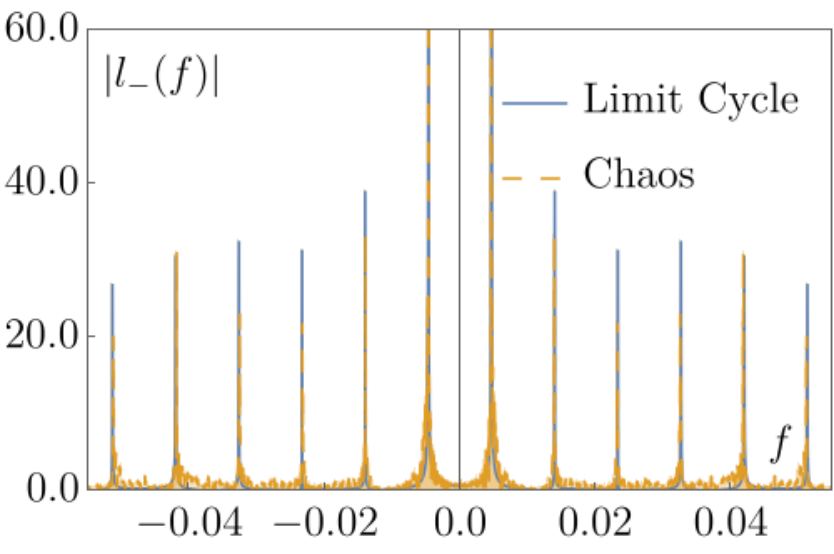
An experimentally observable quantity is the power spectrum, , of the light emitted by the cavity (Patra_1; Carmichael_3). Here is the Fourier transform of the (complex) radiated electric field and is the frequency. Within the mean-field approximation, we find , where and is the total classical spin. The quasiperiodic spectrum (Fig. 3c) has main peaks at , with auxiliary peaks spaced at bunched around them. We did not observe more than two-frequency quasiperiodicity. While it is generally difficult to differentiate between chaotic and quasiperiodic spectra QP_Chaos_Spectra, in our system the latter are visibly discrete. Nevertheless, we do not rely on this feature and use maximum Lyapunov exponents to distinguish quasiperiodicity and chaos in Fig. 2. Note that although the chaotic spectrum is continuous, it features distinct peaks that are independent of the initial conditions (Fig. 3f). In contrast to the spectrum of the synchronized chaotic attractor in Fig. 3i, both chaotic and quasiperiodic power spectra have prominent peaks at the origin and no reflection symmetry.
Near the boundary between Phases II and III in Fig. 2 (red points), we observe synchronized chaos. Since the dynamics in this subregion restore the symmetry, the solutions are confined to the 4D -symmetric submanifold. We write the two constraint relations (independent of initial condition) as
| (6) |
For our purposes, these relations define the synchronization manifold. Coordinates spanning the “transverse manifold” (complementary to the synchronization manifold) are
| (7) |
We derive the evolution equations for the transverse subsystem from Eq. (3) as
| (8a) | |||||
| (8b) | |||||
To compute the conditional Lyapunov exponent for an attractor, we first determine its and with the help of Eq. (3). These serve as time-dependent coefficients in Eqs. (8). In principle, we should linearize Eqs. (8) in small deviations and . However, since these equations are already linear, we simply redefine and to be such arbitrary infenitesimal deviations in transverse directions and numerically simulate Eqs. (8). The conditional Lyapunov exponent is the rate of growth of distances in the transverse manifold, i.e., it is given by Eq. (5), where is the transverse distance. For chaotic synchronized trajectories for , whereas for chaotic ones (Fig. 4). On the other hand, maximum Lyapunov exponents for both chaos and synchronized chaos behave similarly.
In Appendix A, we explain the emergence of the synchronized chaos in our system via tangent bifurcation intermittency of the -symmetric limit cycle. As a result, synchronized chaotic trajectories spend most of their time in the vicinity of the now unstable -symmetric limit cycle, see Fig. 6a. Further, we observe in Fig. 7 that the synchronized chaotic attractor starts off being unstable in the full phase space. Only close to the boundary of the Phases II and III (red points) this attractor becomes sufficiently attractive Chaotic_Synch_X. The restoration of the symmetry explains the reflection symmetric (with no peak at zero) power spectrum of the synchronized chaotic attractor, see Figs. 3i.
In the master equation (1) we neglected the effects of spontaneous emission and inhomogeneous life time . Since the chaotic synchronization is an asymptotic solution of mean-field equations (3), one needs to clarify the effects of these neglected decay processes at large times. To this effect, we show in Fig. 8 that the system reaches its steady state for and (same as in Figs. 3g, 3h, and 3i) in approximately s ( time steps). In a typical experimental setup the timescale related to spontaneous emission can be pushed to s, whereas can be as large as s Holland_One_Ensemble_Theory_1. This comparison of the experimental timescales with the timescale relevant for the observation of chaotic synchronization validates the master equation (1).
Another impediment for the observation of chaotic synchronization is the limited efficiency of the atomic traps that are required to localize the atomic ensembles. Current experiments Holland_One_Ensemble_Expt_1 are able to observe superradiant emission for as long as ms. This should be enough to detect the signature of chaotic synchronization – exponential attenuation of . For example, in Fig. 8 this is seen between and ms. Loss of atoms from the traps with different rates can also lead to atom number imbalance between the ensembles, which in turn breaks the symmetry. This effect, however, affects the steady states only perturbatively, see Fig. 9.
IV Conclusion
In conclusion, we have predicted chaotic synchronization of the dynamics of two atomic ensembles collectively coupled to a heavily damped cavity mode. Synchronized chaos emerges from quasiperiodicity by way of (asymmetric) chaos. Its origin is in the tangent bifurcation intermittency of the -symmetric limit cycle (see Appendix A). We distinguish the three phases theoretically, by analyzing the Poincaré sections and maximum and conditional Lyapunov exponents. Open questions include the effects of coupling to multiple cavity modes and of quantum fluctuations. A quantum analogue to our system, where the overall system is chaotic, but a subsector is not, is known Qtm_Chaos. It would also be interesting to explore prospects of realizing a viable steganography Uchida; Chaotic_Synch_1; Chaotic_Synch_2; Chaotic_Synch_3; Chaotic_Synch_6 (instead of hiding the meaning of transmitted message, hide the existence of the message itself) protocol with our system. In particular, it is not apparent how to send a message over a long distance.
This work was supported by the National Science Foundation Grant DMR1609829.
Appendix A Tangent Bifurcation Intermittency in the -symmetric Submanifold
Recall that the synchronized chaotic attractor spontaneously restores the symmetry between the two ensembles of atoms. Therefore, to gain further insight into it, we investigate -symmetric dynamics in this section.
After a rotation around the z-axis by an angle , which depends on the initial condition, -symmetric dynamics are invariant with respect to the replacement (4), i.e.,
| (9) |
This implies , and the mean-field equations of motion (3) for the spin become
| (10a) | |||||
| (10b) | |||||
| (10c) | |||||
where we dropped the superscript A for simplicity. The spin is related to by Eq. (9).
Note that Eq. (10) is very different from the mean-field equations of motion for a single atomic ensemble coupled to a bad cavity. We obtain the latter from the two-ensemble equations (3) by setting one of the spins, say , to zero. Then, by going into a frame uniformly rotating with frequency , we eliminate from the one-ensemble equations of motion. Thus, single ensemble (one spin) equations correspond to setting in Eq. (3). Indeed, summing Eq. (3) for over and rescaling , and we obtain the one ensemble equations of motion in the rotating frame. This implies that the nonequilibrium phase diagram for a single ensemble is just the vertical, axis of the two-ensemble phase diagram in Fig. 2 with the rescaling . It consists of two fixed points (normal phase and monochromatic superradiance), see Ref. Patra_1 for details. In contrast, Eq. (10) depends on two dimensionless parameters and in an essential way and, consequently, has much richer dynamics as we now discuss.
While solutions of Eq. (10) are consistent with the full mean-field equations (3), their stability in the full phase space is not guaranteed. The three types of solutions of Eq. (10) are: fixed points, periodic ( symmetric limit cycle), and chaotic (synchronized chaos). In the parentheses we mention the equivalent solutions of Eq. (3).
Consider the portion of the phase diagram to the left of the symmetry breaking line (black dashed line) in Fig. 7. Although the -symmetric limit cycle loses stability in the full phase-space, it is still stable on the -symmetric submanifold. As we move towards the Phase II-III boundary, the periodic solution eventually loses stability on the dot-dashed line in Fig. 7 even on the -symmetric submanifold, giving rise to chaos. We determine this line in by computing the maximum Lyapunov exponent with the help of Eqs. (11) and (10). To the left of the dot-dashed line see, e.g., Fig. 6b. Additionally, we prove the loss of stability employing Floquet analysis of Eq. (10).
The abrupt transition, and the proximity of the periodic and chaotic attractors suggest tangent bifurcation intermittency Hilborn. To illustrate this closeness we compare a chaotic spectrum with an adjacent periodic one in Fig. 6c. Below, we provide the final proof in support of this claim by studying the evolution of the Floquet multipliers.
A.1 Floquet Analysis
Our goal is to analyze the stability of the periodic solutions of the reduced equations (10). To that end, we first summarize the Floquet analysis. Write the solution of Eq. (10) as , where is the periodic solution with period , and is a perturbation. Linearizing Eq. (10) with respect to the perturbation, we obtain a set of linear equations with time-dependent coefficients
| (11a) | |||||
| (11b) | |||||
| (11c) | |||||
The next step is to determine the monodromy matrix for Eq. (11). Here is a matrix. Its columns are any three linearly independent solutions of Eq. (11), which we obtain numerically. The eigenvalues of the monodramy matrix are known as Floquet multipliers and are the corresponding Floquet exponents. By Floquet theorem, the general solution of Eq. (11) is
| (12) |
where are constants and are linearly independent and periodic with period vectors. The limit cycle looses stability when the absolute value of one of the Floquet multipliers becomes greater than one.
Further, notice that is a purely periodic with period solution of Eq. (11). This implies that one of the Floquet multipliers is identically equal to one, so that Eq. (12) takes the form
| (13) |
Near the dot-dashed line in Fig. 7, the remaining Floquet multipliers and are both real. As we approach this line from the right, tends to one from below, while remains less than one across criticality.
This behavior of the Floquet multipliers implies (by definition) tangent bifurcation intermittency route to chaos Hilborn. A key feature of this route to chaos is that the chaotic attractor right after the bifurcation remains close to the now unstable limit cycle for most of the time, which we indeed observe in Figs. 6a and 6c. Further, the power spectrum of the -symmetric limit cycle is known to have reflection symmetry and no peak at zero frequency Patra_1. The power spectrum of the synchronized chaotic attractor in Fig. 6c reproduces these features due to the proximity of its trajectory to the limit cycle.
References
- (1) A. Uchida, Optical Communication with Chaotic Lasers (Wiley-VCH, 2012).
- (2) L. M. Pecora, T. L. Carroll, G. A. Johnson, and D. G. Mar, Fundamentals of Synchronization in Chaotic Systems, Concepts and Applications, Chaos 7, 520 (1997).
- (3) L. M. Pecora and T. L. Carroll, Synchronization in Chaotic Systems, Phys. Rev. Lett. 64, 821 (1990).
- (4) S. Hayes, C. Grebogi, E. Ott and A. Mark, Experimental Control of Chaos for Communication, Phys. Rev. Lett. 73, 1781 (1994).
- (5) P. M. Alsing, A. Gavrielides, V. Kovanis, R. Roy and K. S. Thornburg, Jr., Encoding and Decoding Messages with Chaotic Lasers, Phys. Rev. E. 56, 6302 (1997).
- (6) H. G. Winful and L. Rahman, Synchronized Chaos and Spatiotemporal Chaos in Array of Coupled Lasers, Phys. Rev. Lett. 65, 1575 (1990).
- (7) R. Roy and K. S. Thornburg, Jr., Experimental Synchronization of Chaotic Lasers, Phys. Rev. Lett. 72, 2009 (1994).
- (8) T. Fukuyama, R. Kozakov, H. Testrich and C. Wilke, Spatiotemporal Synchronization of Coupled Oscillators in a Laboratory Plasma, Phys. Rev. Lett. 96, 024101 (2006).
- (9) B. Blasius, A. Huppert, and L. Stone, Complex dynamics and phase synchronization in spatially extended ecological systems, Nature 399, 354 (1999).
- (10) M. de Sousa Vieira, Chaos and Synchronized Chaos in an Earthquake Model, Phys. Rev. Lett. 82, 201 (1999).
- (11) J. M. Weiner, K. C. Cox, J. G. Bohnet, and J. K. Thompson, Phase synchronization inside a superradiant laser, Phys. Rev. A 95, 033808 (2017).
- (12) Minghui Xu and M. J. Holland, Conditional Ramsey Spectroscopy with Synchronized Atoms, Phys. Rev. Lett. 114, 103601 (2015).
- (13) Minghui Xu, D. A. Tieri, E. C. Fine, James K. Thompson and M. J. Holland, Synchronization of Two Ensembles of Atoms, Phys. Rev. Lett. 113, 154101 (2014).
- (14) A. Patra, B. L. Altshuler and E. A. Yuzbashyan, Driven-Dissipative Dynamics of Atomic Ensembles in a Resonant Cavity: Nonequilibrium Phase Diagram and Periodically Modulated Superradiance, Phys. Rev. A 99, 033802 (2019).
- (15) H. J. Carmichael, An Open System Approach to Quantum Optics (Springer-Verlag Berlin Heidelberg, 1993).
- (16) W Tucker, Computing Accurate Poincaré Maps, Physica D 171, 127 (2002).
- (17) R. C. Hilborn, Chaos and Nonlinear Dynamics, An Introduction for Scientists and Engineers, Second Edition (Oxford University Press, 2001).
- (18) D. Ruelle and F. Takens, On the Nature of Turbulence, Commun. Math. Phys. 20, 167 (1971).
- (19) S. E. Newhouse, D. Ruelle and F. Takens, Occurance of Strange Axiom A Attractors near Quasi-periodic Flows on , Commun. Math. Phys. 64, 35 (1978).
- (20) R. Bonifacio, P. Schwendimann, and Fritz Haake, Quantum Statistical Theory of Superradiance. I, Phys. Rev. A 4, 302 (1971).
- (21) R. S. Dumont and P. Brumer, Characteristics of power spectra for regular and chaotic systems, J. Chem. Phys. 88, 1481 (1988).
- (22) K. Josić, Invariant Manifolds and Synchronization of Coupled Dynamical Systems, Phys. Rev. Lett. 80, 3053 (1998).
- (23) D. Meiser, Jun Ye, D. R. Carlson and M. J. Holland, Prospects for a Milihertz- Linewidth Laser, Phys. Rev. Lett. 102, 163601 (2006).
- (24) J. G. Bohnet, Z. Chen, J. M. Weiner, D. Meiser, M. J. Holland and J. K. Thompson, A steady-state superradiant laser with less than one intracavity photon, Nature 484, 78 (2012).
- (25) V. A. Yurovsky, Long-lived states with well-defined spins in spin homogeneous Bose gases, Phys. Rev. A 93, 023613 (2016).