Pairing in quantum-critical systems: $T_{c}$, $\Delta$, and their ratio

The BCS theory of superconductivityBardeen et al. 1957a; *BCS2 is rightly considered to be one of the most elegant theoretical works of the 20th century. Not only it explains how to obtain the energy gap in the fermionic spectrum, $\Delta$, and the transition temperature $T_{c}$ as functions of material-dependent parameters, but it also predicts that the ratio $2\Delta/T_{c}=3.53$ is a material-independent universal number. Measurements on ordinary superconductors, like aluminum, did find $2\Delta/T_{c}$ ratio consistent with BCS theory Scalapino 1969 However, in other materials, including novel superconductors, $2\Delta/T_{c}$ is higher. The two obvious reasons, particularly applicable to the cuprates, are non-s-wave superconductivity Maiti and Chubukov 2011; Musaelian et al. 1996 and pseudogap physics Norman et al. 2005. Another potential reason is the sensitivity of $2\Delta/T_{c}$ to strong coupling effects. They are often associated with Mott physics Lee et al. 2006, however a large $2\Delta/T_{c}\sim 8-13$ (depending how $\Delta$ is defined, see below) has been found in Eliashberg calculations of phonon-mediated s-wave superconductivity Scalapino 1969; Carbotte 1990; Marsiglio and Carbotte 1991a; Combescot 1995; Marsiglio and Carbotte 2008, in the limit when, Debye frequency $\omega_{D}$ is vanishingly small, but electron-phonon interaction $g$ is finite (in this limit, both $T_{c}$ and $\Delta$ scale with $g$, Refs. Allen and Dynes 1975; *others1; *others2; *others3).

Phonon-mediated pairing at $\omega_{D}\to 0$ is a specific realization of a more generic situation when the pairing is mediated by a massless boson with susceptibility $\chi(q,\Omega)$, minimally coupled to fermions. Other examples include pairing between fermions at a half-filled Landau level, when a massless boson is a gauge field with Landau overdamped propagator $\chi(q,\Omega)\propto 1/(q^{2}+a|\Omega|/q)$ (e.g., Ref. Bonesteel et al. 1996) and pairing in a metal at the onset of an instability towards a charge or a spin order either with $q=0$ or with a finite lattice momentum,   Abanov et al. 2001; Abanov et al. 2003; Son 1999; Chubukov and Schmalian 2005; Lee 2009; *sslee2; Sachdev et al. 2009; *subir2; Moon and Chubukov 2010; Metlitski and Sachdev 2010a; *max2; Mross et al. 2010; Mahajan et al. 2013; *raghu2; *raghu3; *raghu4; *raghu5; Fradkin et al. 2010; Monthoux et al. 2007; *scal2; Metlitski et al. 2015; Meier et al. 2014; *efetov2; Raghu et al. 2015; Lederer et al. 2015; Bok et al. 2016; Hartnoll et al. 2011; *max_22; *max_23; Maier and Strack 2016; *strack2; Haslinger and Chubukov 2003 The pairing problem in these systems is often considered within the computational scheme similar (but not identical) to the one originally used by Eliashberg in his analysis of phonon-mediated superconductivity Eliashberg 1960. Namely, the fully renormalized pairing vertex is obtained by summing up series of ladder diagrams, like in BCS theory but with dynamical bosonic propagator $\chi(q,\Omega)$, and with fermionic propagators, which include one-loop fermionic self-energy. The latter comes from the same fermion-boson interaction and is computed self-consistently with the pairing vertex. Higher-order self-energy corrections and non-ladder renormalizations of the pairing vertex are assumed to be small [a necessary condition is a requirement that a soft boson is a slow mode compared to a fermion, i.e., for the same momentum, a typical bosonic frequency must be smaller than a typical fermionic frequency]. Within this approximation xxx, the momentum integration in the Eliashberg equations can be performed exactly for a given pairing symmetry com, and the problem reduces to the set of coupled 1D integral equations for frequency dependent pairing vertex $\Phi(\omega)$ and fermionic self-energy $\Sigma(\omega)$Scalapino 1969; Carbotte 1990; Abanov et al. 2001; Abanov et al. 2003; Marsiglio and Carbotte 2008. For spin-singlet pairing, which we consider here, the two equations are, in Matsubara frequencies

Here $\chi_{L}(\Omega_{m})$ is the effective, local, dimensionless bosonic susceptibility (it is equal to $g^{2}\chi(q,\Omega_{m})$ integrated over Fermi surface with form-factors for a given pairing channel $s$, $p$, $d$, etc). For electron-phonon problem at vanishing Debye frequency, $\chi_{L}(\Omega)=g^{2}/|\Omega_{m}|^{2}$. We consider a generic model with $\chi_{L}(\Omega)=g^{\gamma}/|\Omega_{m}|^{\gamma}$ — the $\gamma$ model. For a nematic and Ising-ferromagnetic critical points $\gamma=1-D/3$, where $D$ is a spatial dimension, for antiferromagnetic critical point $\gamma=(3-D)/2$, models with other values of $\gamma$ have also been identifiedSon 1999; Chubukov and Schmalian 2005; Altshuler et al. 1995; Wang and Chubukov 2013; Bergeron et al. 2012. A similar set of equations for the frequency dependent pairing vertex and fermionic self-energy emerges in the dynamical mean-field theory (DMFT) approach, and it was argued that for DMFT analysis of a Hund metal within three-band Hubbard model for Fe-based superconductors yields $\chi_{l}(\Omega)\propto 1/|\Omega|^{1.2}$ in a wide range of frequenciesStadler et al. 2015; Lee et al. 2018. As additional complication, the form of $\chi_{L}(\Omega)$ may by itself depend on $\Phi$ due to feedback from superconductivity on the bosonic propagator Abanov and Chubukov 1999; Eschrig 2006 This can be incorporated by treating $\gamma$ below $T_{c}$ as temperature-dependent parameter.

The goal of our study is to extract some new physics from the analysis of $2\Delta/T_{c}$ in the $\gamma$-model. The pairing gap $\Delta(\omega_{n})$ is related to the pairing vertex as $\Delta(\omega_{n})=\Phi(\omega_{n})/(1+\Sigma(\omega_{n})/\omega_{n})$, and the Eliashberg equation for $\Delta(\omega_{n})$ is

The $T_{c}$ is obtained as the highest temperature at which Eq. (2) has a solution. Note that the term with $m=n$ in the r.h.s. of (2) (the self-action term) can be neglected due to vanishing of the numerator. To see this more clearly, one has to add a small mass term $M$ to the interaction and take the limit $M\to 0$ only at the end of calculations. The numerator in (2) vanishes at $m=n$ for any $M$. This vanishing is the consequence of the cancellation between the contributions to the gap equation from the renormalization of the pairing vertex and the self-energy Millis et al. 1988; Wang et al. 2016; Abanov et al. 2008, and it has the same physics origin as the Anderson theorem – the independence of $T_{c}$ on non-magnetic impuritiesAnderson 1959. Indeed, the term with $m=n$ describes the scattering with zero frequency transfer, averaged over finite momentum transfers, i.e., its role in the gap equation is equivalent to that of elastic scattering by non-magnetic impurities. We remind in this regard that we consider spin-singlet pairing. For spin-triplet pairing, the r.h.s. of the equation for the pairing vertex contains the extra overall factor $-1/3$, and the term with $m=n$ does not vanish, in analogy with the case when impurities are magnetic Wang et al. 2001; *triplet2; *triplet3

For the gap $\Delta$ at $T=0$ we will use $\Delta_{0}=\Delta(\pi T)$ at the lowest temperature. One can show that $\Delta_{0}=\Delta(\omega=0)$ on the real axis. An alternative is to associate $\Delta$ with the frequency at which the density of states has a maximum, $\Delta_{\text{DOS}}$. In BCS theory $\Delta_{0}=\Delta_{\text{DOS}}$ and $2\Delta_{0}/T_{c}=3.53$, but in the $\gamma$ model, $\Delta_{\text{DOS}}>\Delta_{0}$. In a phonon superconductor with $\omega_{D}=0$, $\Delta_{\text{DOS}}\approx(\pi/2)\Delta_{0}$. This accounts for the discrepancy in reported $2\Delta/T_{c}$ ratio: $2\Delta_{0}/T_{c}\sim 8.3$, while $2\Delta_{\text{DOS}}/T_{c}\sim 12.9$ (Refs. Scalapino 1969; Carbotte 1990).

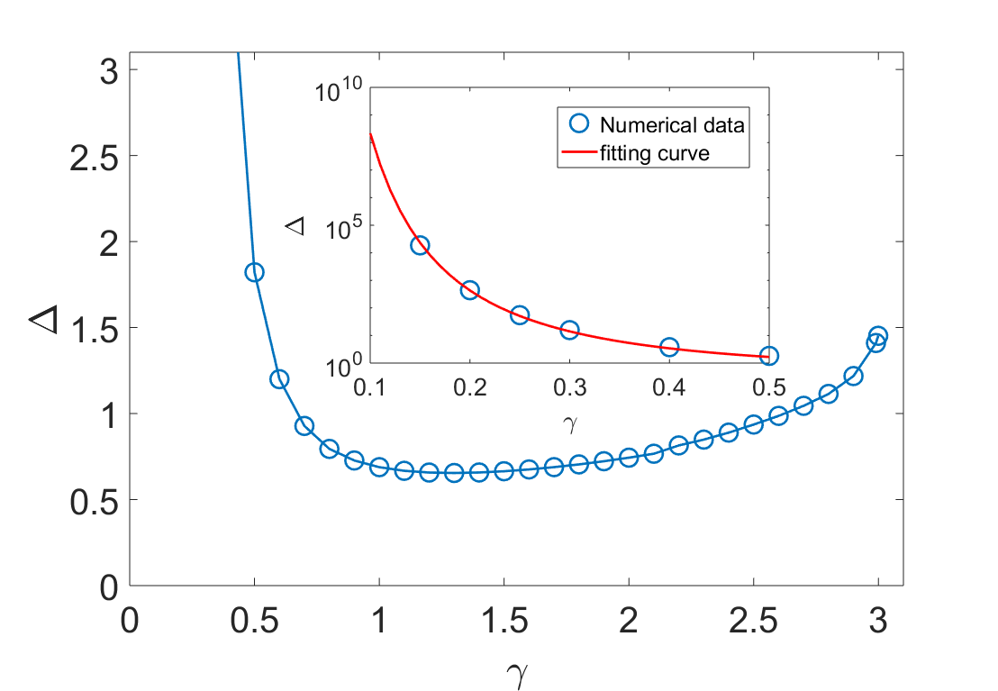
The ratio of $2\Delta/T_{c}$ in the $\gamma$ model has been recently analyzed numerically for $0<\gamma\leq 2$ and was found to increase rapidly with increasing $\gamma$Lee et al. 2018. We obtained the same result (see Fig.3) and also found that the increase of $2\Delta/T_{c}$ accelerates at larger $\gamma$. The goal of our work is to provide an explanation for the increase. We argue that $2\Delta/T_{c}$ actually diverges at $\gamma\to 3$. The divergence is the direct consequence of the fact that at $T=0$, when Matsubara frequencies become continuous variables, the integral in the r.h.s. of the gap equation (2) becomes singular at $\omega_{m}\approx\omega_{n}$ ($\int dxx^{2}/|x|^{\gamma}$ diverges at $\gamma\geq 3$). We obtain analytical formulas for $T_{c}$ and $\Delta$ near $\gamma=3$ and argue that they remain valid in a wide range of $\gamma<3$.

Another goal of our study is to analyze the opposite limit of small $\gamma$. Here we explore the fact that for any $\gamma>0$, $\chi_{L}(\Omega)=(g/|\Omega|)^{\gamma}$ is a decreasing function of $\Omega$, in which case the r.h.s. of the gap equation is ultra-violet convergent, and there is no need to impose an upper cutoff in the frequency summation in (2). We obtain the explicit expressions for $T_{c}$ and $\Delta$ in the small $\gamma$ limit. We show that $T_{c}=Q_{T}\omega_{0}$ and $\Delta=Q_{\Delta}\omega_{0}$, where $\omega_{0}=g(1.4458\gamma)^{1/\gamma}$ and $Q_{T}$ and $Q_{\Delta}$ are are numerical factors of order one. The scale $\omega_{0}$ has been identified before Metlitski et al. 2015 To obtain it, one can neglect fermionic self-energy, i.e., treat fermions as free quasiparticles, like in BCS theory. However, to obtain the factors $Q_{T}$ and $Q_{\Delta}$ one need to include the subleading terms in $\gamma$, and these additional terms do depend on the non-Fermi liquid self-energy $\Sigma(\omega)\propto\omega^{1-\gamma}_{m}$. We show that the self-energy contributions to $Q_{T}$ and $Q_{\Delta}$ are rather non-trivial, and the result is very different from the one in a weakly coupled Fermi liquid, where the self-energy changes the exponential factor $e^{-1/\lambda}$ into $e^{-(1+\lambda)/\lambda}=e^{-1/\lambda}/e$ (Refs. Dolgov et al. 2005; Wang and Chubukov 2013; Marsiglio 2018 Still, we show that self-energy equally affects $T_{c}$ and $\Delta$, such that $2Q_{\Delta}/Q_{T}=3.53$, as in BCS theory. We computed $T_{c}$ and $\Delta$ numerically at small $\gamma$, and found good agreement with our analytical results.

The structure of the paper is as follows. In Sec. II we briefly review how $\Delta$ and $T_{c}$ are obtained in BCS theory. In Sec.III we study the case when $\gamma$ is small and obtain explicit formulas for both $T_{c}$ and $\Delta$. The prefactors $Q_{T}$ and $Q_{D}$ are calculated both analytically and numerically. In Sec.IV we show the divergence of $\Delta$ when $\gamma\to 3$.

To set the stage for our calculations, we briefly outline how $2\Delta/T_{c}$ is obtained in BCS theory. Here, $\chi_{L}(\Omega)=\lambda$ is frequency independent, and $\Delta(\omega_{n})=\Delta$. The frequency sum in the gap equation diverges at large ${}\omega_{m}$ and one has to set the upper cutoff $\Lambda$. We then have

where $Li(z)=\int_{0}^{z}dx/\log{x}$ is a logarithmic integral. Using $Li\left(3/2+\Lambda/(2\pi T)\right)-Li\left(1/2)\right)=\log{2e^{C}\Lambda/(\pi T)}$, where $C=0.577216$ is the Euler’s constant, we immediately obtain $T_{c}=(2e^{C}\Lambda/\pi)e^{-1/\lambda}$, $\Delta=(2\Lambda)e^{-1/\lambda}$, and $2\Delta/T_{c}=2\pi/e^{C}=3.52775$. In Eliashberg theory with $\chi_{L}=\lambda$ one also has to include the self-energy $\Sigma=\lambda\omega$, Eq. (I), and then $T_{c}=(2e^{C-1}\Lambda/\pi)e^{-1/\lambda}$, $\Delta=(2\Lambda/e)e^{-1/\lambda}$. The ratio $2\Delta/T_{c}$ still remains $3.53$.

We first consider the case when $\chi_{L}(\Omega)=(g/|\Omega|)^{\gamma}$ with small but finite $\gamma$. As we said, for any finite $\gamma$, the paring kernel $\chi_{L}(\omega_{n}-\omega_{m})/|\omega_{m}|$ decreases faster than $1/|\omega_{m}|$, i.e., frequency summation over $m$ in the r.h.s. of the gap equation (2) converges. This eliminates the need to introduce an upper frequency cutoff $\Lambda$, that is $T_{c}$ and $\Delta$ remain finite even when $\Lambda$ is infinite.

The small $\gamma$ limit has been considered before. Previous studies analyzed the pairing susceptibility at $T=0$ and identified the large scale $\omega_{0}=g(1.4458\gamma)^{-1/\gamma}\gg g$, at which this susceptibility diverges. We obtain $T_{c}\sim\omega_{0}$ explicitly by solving the linearized gap equation at a finite $T$ and non-linear gap equation at $T=0$, and find the proportionality factors.

We now consider the $\gamma$ model with exponent $\gamma>1$. We show that the ratio $2\Delta/T_{c}$ increases with $\gamma$ and diverges at $\gamma=3$. We argue that this divergence is the primary reason why earlier works Scalapino 1969; Carbotte 1990; Combescot 1995; Marsiglio and Carbotte 2008 found a very large (but finite) $2\Delta/T_{c}$ by solving Eliashberg equations for a phonon superconductor with effective phonon-mediated pairing interaction $g^{2}/(\Omega^{2}+\omega^{2}_{D})$ in the limit when the Debye frequency vanishes, but the coupling $g$ remains finite (the corresponds to $\gamma=2$ in our notations).

In this paper we analyzed superconducting $T_{c}$ and $2\Delta/T_{c}$ ratio in a metal at the verge of an instability towards a spin or a charge order. Near the instability, the dominant interaction between fermions is the exchange of soft bosonic fluctuations of spin or charge order parameter. In spatial dimension $D\leq 3$ this interaction gives rise to a non-Fermi liquid behavior either on a whole Fermi surface or in hot regions, but also provides a strong attraction in at least one pairing channel. We considered a subset of such systems, in which soft bosons can be regarded as slow modes compared to electrons, and the pairing can be treated within Eliashberg theory with an effective local interaction $\chi_{L}(\Omega_{m})=\left(g/|\Omega_{m}|\right)^{\gamma}$ (the $\gamma$ model). The same effective theory emerges for the pairing between fermions at the half-filled Landau level and in models studied within DMFT.

The $\gamma$ model with $\gamma=2$ describes electron-phonon superconductivity in the special limit when Debye frequency vanishes but fermion-boson coupling $g$ remains finite, i.e., the boson-mediated interaction is $(g/|\Omega|)^{2}$. This problem has been extensively studied in the past  Scalapino 1969; Allen and Dynes 1975; *others1; *others2; *others3; Carbotte 1990; Combescot 1995; Marsiglio and Carbotte 2008. It was well established that $T_{c}\approx 0.18g$ and $\Delta(0)\approx 0.75g$ remain finite, but their ratio $2\Delta/T_{c}\approx 8.3$ is much larger than in BCS theory. T-H Lee et al recently analyzed numerically $2\Delta/T_{c}$ in the $\gamma$-model for $\gamma<2$ (Ref. Lee et al. 2018) and found that the ratio monotonically increases with increasing $\gamma$.

One goal of our work was to provide an explanation for this increase. We considered a larger range of $\gamma\leq 3$ and found that $2\Delta(0)/T_{c}$ diverges at $\gamma\to 3$ ($T_{c}$ remains finite in this limit, but $\Delta_{0}$ diverges). We obtained analytical formulas for $T_{c}$ and $\Delta$ near $\gamma=3$ and argued that they remain valid in a relatively wide range of $\gamma<3$. We also computed $T_{c}$ and $\Delta$ numerically and found good agreement between analytical and numerical results.

Another goal of our work was to analyze the opposite limit of small $\gamma$. Here we obtained the exact expressions for $T_{c}$ and $\Delta$ with numerical prefactors. We emphasize that for any non-zero $\gamma$, the normal state self-energy has a non-Fermi liquid form at small frequencies, and non-Fermi-liquid behavior does affect the values of $T_{c}$ and $\Delta$.

A word of caution. In our analysis we focused on the solution of the linearized gap equation with the highest $T_{c}$ and on the ”conventional” solution of the non-linear equation at $T=0$, for which $\Delta(\omega_{m})$ is a regular function of frequency with no sign changes. There exist other solutions of the gap equation, for which $\Delta(\omega_{m})$ oscillates. For $\gamma<2$, there is little doubt that the conventional solution with no-nodal $\Delta(\omega_{m})$ has the largest condensation energy. However, for $\gamma>2$, it is possible that the largest condensation energy is for an unconventional solution with oscillating $\Delta(\omega_{m})$ (Ref.Abanov_new). This would affect the ratio of $2\Delta/T_{c}$. Still, even if this is the case, our analysis is applicable to $\gamma\leq 2$, and it explains why $2\Delta/T_{c}$ increases with $\gamma$. Also, $T_{c}$ in our analysis is the onset temperature for the pairing instability. In the absence of fluctuations it coincides with the actual superconducting $T_{c}$, but when fluctuations are present, the actual $T_{c,act}$ likely gets smaller, while our mean-field $T_{c}$ marks the onset of pseudogap behavior. Our $2\Delta/T_{c}$ should then be understood as the ratio of the gap at $T=0$ to the onset temperature for pseudogap behavior. And, finally, in our analysis we neglected the feedback from the gap opening on the form of $\chi_{L}(\Omega)$ (e.g., the development of the resonant peak in the spin-fluctuation propagator due to the opening of $d-$wave or $s^{+-}$ gap). Within the $\gamma$ model this last effect can be captured by allowing $\gamma$ to vary with $T$ below $T_{c}$ towards a smaller value.

References

- Bardeen et al. (1957a) J. Bardeen, L. N. Cooper, and J. R. Schrieffer, Phys. Rev. 106, 162 (1957a).
- Bardeen et al. (1957b) J. Bardeen, L. N. Cooper, and J. R. Schrieffer, Phys. Rev. 108, 1175 (1957b).
- Scalapino (1969) D. Scalapino, in Superconductivity, edited by R. Parks (CRC Press, 1969).
- Maiti and Chubukov (2011) S. Maiti and A. V. Chubukov, Phys. Rev. B 83, 220508 (2011).
- Musaelian et al. (1996) K. A. Musaelian, J. Betouras, A. V. Chubukov, and R. Joynt, Phys. Rev. B 53, 3598 (1996).
- Norman et al. (2005) M. R. Norman, D. Pines, and C. Kallin, Advances in Physics 54, 715 (2005).
- Lee et al. (2006) P. A. Lee, N. Nagaosa, and X.-G. Wen, Rev. Mod. Phys. 78, 17 (2006).
- Carbotte (1990) J. P. Carbotte, Rev. Mod. Phys. 62, 1027 (1990).
- Marsiglio and Carbotte (1991a) F. Marsiglio and J. P. Carbotte, Phys. Rev. B 43, 5355 (1991a).
- Combescot (1995) R. Combescot, Phys. Rev. B 51, 11625 (1995).
- Marsiglio and Carbotte (2008) F. Marsiglio and J. P. Carbotte, “Electron-phonon superconductivity,” in Superconductivity: Conventional and Unconventional Superconductors, edited by K. H. Bennemann and J. B. Ketterson (Springer Berlin Heidelberg, Berlin, Heidelberg, 2008) pp. 73–162.
- Allen and Dynes (1975) P. B. Allen and R. C. Dynes, Phys. Rev. B 12, 905 (1975).
- Bergmann and Rainer (1973) G. Bergmann and D. Rainer, Zeitschrift für Physik 263, 59 (1973).
- Marsiglio and Carbotte (1991b) F. Marsiglio and J. P. Carbotte, Phys. Rev. B 43, 5355 (1991b).
- Karakozov et al. (1991) A. Karakozov, E. Maksimov, and A. Mikhailovsky, Solid State Communications 79, 329 (1991).
- Bonesteel et al. (1996) N. E. Bonesteel, I. A. McDonald, and C. Nayak, Phys. Rev. Lett. 77, 3009 (1996).
- Abanov et al. (2001) A. Abanov, A. V. Chubukov, and A. M. Finkel’stein, EPL (Europhysics Letters) 54, 488 (2001).
- Abanov et al. (2003) A. Abanov, A. V. Chubukov, and J. Schmalian, Advances in Physics 52, 119 (2003).
- Son (1999) D. T. Son, Phys. Rev. D 59, 094019 (1999).
- Chubukov and Schmalian (2005) A. V. Chubukov and J. Schmalian, Phys. Rev. B 72, 174520 (2005).
- Lee (2009) S.-S. Lee, Phys. Rev. B 80, 165102 (2009).
- Dalidovich and Lee (2013) D. Dalidovich and S.-S. Lee, Phys. Rev. B 88, 245106 (2013).
- Sachdev et al. (2009) S. Sachdev, M. A. Metlitski, Y. Qi, and C. Xu, Phys. Rev. B 80, 155129 (2009).
- Moon and Sachdev (2009) E. G. Moon and S. Sachdev, Phys. Rev. B 80, 035117 (2009).
- Moon and Chubukov (2010) E.-G. Moon and A. Chubukov, Journal of Low Temperature Physics 161, 263 (2010).
- Metlitski and Sachdev (2010a) M. A. Metlitski and S. Sachdev, Phys. Rev. B 82, 075127 (2010a).
- Metlitski and Sachdev (2010b) M. A. Metlitski and S. Sachdev, Phys. Rev. B 82, 075128 (2010b).
- Mross et al. (2010) D. F. Mross, J. McGreevy, H. Liu, and T. Senthil, Phys. Rev. B 82, 045121 (2010).
- Mahajan et al. (2013) R. Mahajan, D. M. Ramirez, S. Kachru, and S. Raghu, Phys. Rev. B 88, 115116 (2013).
- Fitzpatrick et al. (2013) A. L. Fitzpatrick, S. Kachru, J. Kaplan, and S. Raghu, Phys. Rev. B 88, 125116 (2013).
- Fitzpatrick et al. (2014) A. L. Fitzpatrick, S. Kachru, J. Kaplan, and S. Raghu, Phys. Rev. B 89, 165114 (2014).
- Torroba and Wang (2014) G. Torroba and H. Wang, Phys. Rev. B 90, 165144 (2014).
- Fitzpatrick et al. (2015) A. L. Fitzpatrick, G. Torroba, and H. Wang, Phys. Rev. B 91, 195135 (2015), and references therein.
- Fradkin et al. (2010) E. Fradkin, S. A. Kivelson, M. J. Lawler, J. P. Eisenstein, and A. P. Mackenzie, Annual Review of Condensed Matter Physics 1, 153 (2010).
- Monthoux et al. (2007) P. Monthoux, D. Pines, and G. G. Lonzarich, Nature 450, 1177 (2007).
- Scalapino (2012) D. J. Scalapino, Rev. Mod. Phys. 84, 1383 (2012).
- Metlitski et al. (2015) M. A. Metlitski, D. F. Mross, S. Sachdev, and T. Senthil, Phys. Rev. B 91, 115111 (2015).
- Meier et al. (2014) H. Meier, C. Pépin, M. Einenkel, and K. B. Efetov, Phys. Rev. B 89, 195115 (2014).
- Efetov (2015) K. B. Efetov, Phys. Rev. B 91, 045110 (2015).
- Raghu et al. (2015) S. Raghu, G. Torroba, and H. Wang, Phys. Rev. B 92, 205104 (2015).
- Lederer et al. (2015) S. Lederer, Y. Schattner, E. Berg, and S. A. Kivelson, Phys. Rev. Lett. 114, 097001 (2015).
- Bok et al. (2016) J. M. Bok, J. J. Bae, H.-Y. Choi, C. M. Varma, W. Zhang, J. He, Y. Zhang, L. Yu, and X. J. Zhou, Science Advances 2 (2016), 10.1126/sciadv.1501329.
- Hartnoll et al. (2011) S. A. Hartnoll, D. M. Hofman, M. A. Metlitski, and S. Sachdev, Phys. Rev. B 84, 125115 (2011).
- Hartnoll et al. (2014) S. A. Hartnoll, R. Mahajan, M. Punk, and S. Sachdev, Phys. Rev. B 89, 155130 (2014).
- Chubukov et al. (2014) A. V. Chubukov, D. L. Maslov, and V. I. Yudson, Phys. Rev. B 89, 155126 (2014).
- Maier and Strack (2016) S. A. Maier and P. Strack, Phys. Rev. B 93, 165114 (2016).
- Ridgway and Hooley (2015) S. P. Ridgway and C. A. Hooley, Phys. Rev. Lett. 114, 226404 (2015).
- Haslinger and Chubukov (2003) R. Haslinger and A. V. Chubukov, Phys. Rev. B 68, 214508 (2003).
- Eliashberg (1960) G. M. Eliashberg, JETP 11, 696 (1960).
- (50) In several systems the corrections to Eliashberg formula for the self-energy are singular at the lowest frequencies. In this case, Eliashberg theory is valid if is higher than a typical frequency at which these singular raghucorrections become regular.
- (51) In the cases, when the interaction is peaked for fermions in hot regions on the Fermi surface, the dependence of the pairing vertex and the self-energy on the angle along the Fermi surface is coupled to frequency dependence, and, strictly speaking, one has to solve the set of two 2D coupled integral equations for and . This does not lead to qualitative changes in the value compared to the corresponding models, in which and assumed to be independent on at frequencies relevant to , but may affect ratio.
- Altshuler et al. (1995) B. L. Altshuler, L. B. Ioffe, and A. J. Millis, Phys. Rev. B 52, 5563 (1995).
- Wang and Chubukov (2013) Y. Wang and A. Chubukov, Phys. Rev. B 88, 024516 (2013).
- Bergeron et al. (2012) D. Bergeron, D. Chowdhury, M. Punk, S. Sachdev, and A.-M. S. Tremblay, Phys. Rev. B 86, 155123 (2012).
- Stadler et al. (2015) K. M. Stadler, Z. P. Yin, J. von Delft, G. Kotliar, and A. Weichselbaum, Phys. Rev. Lett. 115, 136401 (2015).
- Lee et al. (2018) T.-H. Lee, A. Chubukov, H. Miao, and G. Kotliar, arXiv 1805, 10280 (2018).
- Abanov and Chubukov (1999) A. Abanov and A. V. Chubukov, Phys. Rev. Lett. 83, 1652 (1999).
- Eschrig (2006) M. Eschrig, Advances in Physics 55, 47 (2006).
- Millis et al. (1988) A. J. Millis, S. Sachdev, and C. M. Varma, Phys. Rev. B 37, 4975 (1988).
- Wang et al. (2016) Y. Wang, A. Abanov, B. L. Altshuler, E. A. Yuzbashyan, and A. V. Chubukov, Phys. Rev. Lett. 117, 157001 (2016).
- Abanov et al. (2008) A. Abanov, A. V. Chubukov, and M. R. Norman, Phys. Rev. B 78, 220507 (2008).
- Anderson (1959) P. Anderson, Journal of Physics and Chemistry of Solids 11, 26 (1959).
- Wang et al. (2001) Z. Wang, W. Mao, and K. Bedell, Phys. Rev. Lett. 87, 257001 (2001).
- Roussev and Millis (2001) R. Roussev and A. J. Millis, Phys. Rev. B 63, 140504 (2001).
- Chubukov et al. (2003) A. V. Chubukov, A. M. Finkel’stein, R. Haslinger, and D. K. Morr, Phys. Rev. Lett. 90, 077002 (2003).
- Dolgov et al. (2005) O. V. Dolgov, I. I. Mazin, A. A. Golubov, S. Y. Savrasov, and E. G. Maksimov, Phys. Rev. Lett. 95, 257003 (2005).
- Marsiglio (2018) F. Marsiglio, Phys. Rev. B 98, 024523 (2018).
- Chubukov and Maslov (2012) A. V. Chubukov and D. L. Maslov, Phys. Rev. B 86, 155136 (2012).