Transitioning from equal-time to light-front quantization
in $\phi_{2}^{4}$ theory

Sophia S. Chabysheva Note: Present address: Department of Physics, University of Idaho, Moscow ID 83844 USA Affiliation: Department of Physics and Astronomy
University of Minnesota-Duluth
Duluth, Minnesota 55812 John R. Hiller^a Affiliation: Department of Physics and Astronomy
University of Minnesota-Duluth
Duluth, Minnesota 55812

August 11, 2026

Abstract

We use the interpolating coordinates studied by Hornbostel to investigate a transition from equal-time quantization to light-front quantization, in the context of two-dimensional $\phi^{4}$ theory. A consistent treatment is found to require careful consideration of vacuum bubbles, in a nonperturbative extension of the analysis by Collins. Numerical calculations of the spectrum at fixed box size are shown to yield results equivalent to those of equal-time quantization, except when the interpolating coordinates are pressed toward the light-front limit. In that regime, a fixed box size is inconsistent with an accurate representation of vacuum-bubble contributions and causes a spurious divergence in the spectrum. The light-front limit instead requires the continuum momentum-space limit of infinite box size. The calculation of the vacuum energy density is then shown to be independent of the interpolation parameter, which implies that the light-front limit yields the same spectrum as an equal-time calculation. This emphasizes the importance of zero modes and near-zero modes in a light-front analysis of any theory with nontrivial vacuum structure.

I Introduction

Recently, there has been a resurgence of interest in the spectrum of two-dimensional $\phi^{4}$ theory Hogervorst; RychkovVitale; Rychkov; Pelissetto; DePalma; Bajnok; BCH; Christensen; Katz1; Katz2; Katz3; Katz4; Serone; Kadoh; Romatschke,¹¹ 1 For citations of older work, see Katz1. partly because of what appeared to be an inconsistency between results from equal-time quantization and light-front quantization. Although the apparent inconsistency has been resolved, as a difference in mass renormalizations SineGordon; BCH; Katz1; Katz3, there remain various issues related to the structure of the vacuum. In light-front quantization BPP; Burkardt; Hiller, the vacuum is famously trivial,²² 2 See, however, the remarks by Collins Collins; Martinovic and Dorokhov Martinovic; and Mannheim, Lowdon, and Brodsky MLB on nontrivial aspects. but in equal-time quantization, it is as complex as any of the other eigenstates.

More specifically, a direct quantitative check of the difference in mass renormalizations BCH was not completely successful and required extrapolation of the light-front mass renormalization from weaker coupling. In Katz3 this failure is attributed³³ 3 See the discussion in Sec. 2.2 of Katz3. to an incomplete nonperturbative formulation of the mass renormalization itself. The mass renormalization relies on a computation of the expectation value $\langle\phi^{2}\rangle$ for the square of the field $\phi$ , which is done with a spectral decomposition. The mass spectrum that was used in BCH lacked the correct behavior near the critical coupling. This caused the incorrect behavior for the computed value of $\langle\phi^{2}\rangle$ and created the need for extrapolation. The incorrect behavior for $\langle\phi^{2}\rangle$ found in Katz3 may also be a numerical artifact that misrepresents the underlying theory. A better understanding requires an improved treatment of vacuum effects in light-front calculations.

In order to see more clearly what may be happening for the light-front vacuum, we apply the interpolation procedure championed by Hornbostel Hornbostel⁴⁴ 4 There are earlier applications of interpolation, to two-dimensional QCD Frishman, the Dirac equation Ahluwalia, and perturbation theory Sawicki, as well as of quantizations close to the light-cone Chen; Elizalde applied to two-dimensional QED and QCD Franke; Lenz. and emphasized by Ji Ji, in which the (two-dimensional) coordinates are chosen to be⁵⁵ 5 This coordinate transformation is not a Lorentz transformation, which makes the $c\rightarrow 0$ limit technically distinct from the infinite-momentum-frame limit IMF.

x^{\pm}=\frac{1}{\sqrt{2}}[\sqrt{1\pm c}t\pm\sqrt{1\mp c}z],

(1)

with $x^{+}$ chosen as the time coordinate. The parameter $c$ ranges from 0 to 1, with 0 being the light-front limit Dirac,⁶⁶ 6 Contrary to our usual convention but in keeping with an equally common choice, $x^{\pm}$ include a factor of $1/\sqrt{2}$ . This matches Hornbostel’s construction Hornbostel and simplifies some of the expressions. where $x^{\pm}=(t\pm z)/\sqrt{2}$ , and 1 the equal-time limit, where $x^{+}=t$ and $x^{-}=-z$ . The minus sign for the equal-time spatial coordinate may seem incongruous, but it is a permissible choice that simplifies the notation.

The conjugate energy and momentum are

p_{\pm}=\frac{1}{\sqrt{2}}[\sqrt{1\pm c}E\mp\sqrt{1\mp c}p_{z}].

(2)

Dot products of the momentum and spatial two-vectors are then given by $p\cdot x=p_{+}x^{+}+p_{-}x^{-}$ . The mass-shell condition becomes

\mu^{2}=E^{2}-p_{z}^{2}=cp_{+}^{2}-cp_{-}^{2}+2sp_{+}p_{-},

(3)

with $s\equiv\sqrt{1-c^{2}}$ . The positive root for $p_{+}$ yields

p_{+}=[\sqrt{p_{-}^{2}+c\mu^{2}}-sp_{-}]/c.

(4)

For the $c=1$ and $c=0$ limits, this expression becomes

p_{+}\rightarrow\left\{\begin{array}[]{ll}\sqrt{p_{z}^{2}+\mu^{2}},&c=1\\ \frac{\mu^{2}}{2p_{-}}=\frac{\mu^{2}}{2p^{+}},&c=0,p_{-}>0\\ \frac{\mu}{\sqrt{c}},&c\rightarrow 0,p_{-}=0\\ \frac{2|p_{-}|}{c},&c\rightarrow 0,p_{-}<0.\end{array}\right.

(5)

Clearly, the zero modes ( $p_{-}=0$ ) and negative $p_{-}$ states have infinite light-front energy and are removed from the spectrum, as $c\rightarrow 0$ .

However, these modes can contribute to light-front computations and, in particular, to vacuum expectation values Hornbostel; Ji. A standard illustration of this is in the spectrum and VEV of a free scalar field that has been shifted by a constant. The shift introduces to the Lagrangian a term that is linear in the field; this contributes a term to the Hamiltonian that is proportional to the spatial average of the field, a constant that must be built from zero modes absent in ordinary light-front calculations. The recovery of the contribution can be seen quite clearly in the $c\rightarrow 0$ limit, where the Hamiltonian eigenvalue problem in an $x^{-}$ box has an analytic solution for any $c>0$ . A numerical solution in a truncated Fock space works just as well. This is discussed in Sec. II.

For $\phi^{4}$ theory, the zero-mode contribution is more subtle. We expand upon the perturbative analysis of Collins Collins to illustrate how zero-mode contributions to the self-energy corrections are missed by the standard light-front analysis yet survive the $c\rightarrow 0$ limit. In Sec. III, we will explore what the solutions with $c\neq 0$ and the $c\rightarrow 0$ limit can tell us. The calculations are done numerically, in a Fock basis of discrete momentum states in an $x^{-}$ box. These lead to a much better understanding of the $c\rightarrow 0$ limit. A fixed box size is shown to be inconsistent with this limit. Instead, one must consider the continuum limit simultaneously with the light-front limit. A summary of these observations and our conclusions is given in Sec. IV.

II Shifted free scalar

A free scalar field that is shifted by a constant provides an interesting example of the impact of zero modes on a light-front calculation. This can be seen explicitly in the $c\rightarrow 0$ limit, where a nonzero contribution is found for the vacuum energy and the VEV of the field. These analytic results Hornbostel; Ji can be replicated in a numerical calculation using a Fock basis of zero modes. We illustrate this here.

The Lagrangian of a free scalar field of mass $\mu$ is

{\cal L}_{0}=\frac{1}{2}\partial_{\mu}\phi\partial^{\mu}\phi-\frac{1}{2}\mu^{2}\phi^{2}.

(6)

In terms of the interpolating coordinates (1), with arbitrary $c$ and in two dimensions, this becomes Hornbostel

{\cal L}_{0}=\frac{1}{2}c[(\partial_{+}\phi)^{2}-(\partial_{-}\phi)^{2}]+s\partial_{+}\phi\partial_{-}\phi-\frac{1}{2}\mu^{2}\phi^{2}.

(7)

The (free) Hamiltonian is

{\cal P}_{+}^{0}=\int dx^{-}(\pi\partial_{+}\phi-{\cal L}_{0}),

(8)

with $\pi=c\partial_{+}\phi+s\partial_{-}\phi$ and $s=\sqrt{1-c^{2}}$ . The mode expansion for the field is

\phi=\int_{-\infty}^{\infty}\frac{dp_{-}}{\sqrt{4\pi w_{p}}}[a(p_{-})e^{-ip\cdot x}+a^{\dagger}(p_{-})e^{ip\cdot x}],

(9)

with $w_{p}\equiv\sqrt{p_{-}^{2}+c\mu^{2}}$ . The nonzero commutation relation is

[a(p_{-}),a^{\dagger}(p^{\prime}_{-})]=\delta(p_{-}-p^{\prime}_{-}).

(10)

The normal-ordered free Hamiltonian can then be written as

{\cal P}_{+}^{0}=\int_{-\infty}^{\infty}dp_{-}p_{+}a^{\dagger}(p_{-})a(p_{-})=\int_{-\infty}^{\infty}dp_{-}\frac{w_{p}-sp_{-}}{c}a^{\dagger}(p_{-})a(p_{-}).

(11)

Similarly, the momentum operator is

{\cal P}_{-}=\int_{-\infty}^{\infty}dp_{-}\,p_{-}\,a^{\dagger}(p_{-})a(p_{-}).

(12)

Discretization consistent with discrete light-cone quantization (DLCQ) PauliBrodsky is invoked by placing the system in a box $-L<x^{-}<L$ with periodic boundary conditions. The momentum is then discrete, $p_{-}=n\pi/L$ , as set by the integer $n$ ; however, unlike DLCQ, $n$ ranges over all integers, not just the positive ones.⁷⁷ 7 As shown in the last line of (5), negative $p_{-}$ is removed from the spectrum only on the light front, at $c=0$ . An energy cutoff is then required for a finite basis, just as for an ordinary equal-time calculation. We do still define a positive integer $K$ as the resolution PauliBrodsky, so that in the $c\rightarrow 0$ light-front limit, the total momentum is $P_{-}=K\pi/L$ . The index $n$ for individual momentum then ranges from 1 to $K$ in the light-front limit, and momentum fractions $p_{-}/P_{-}$ are just $n/K$ .

The discrete mode expansion for arbitrary $c$ is

\phi(x^{+}=0)=\sum_{n=-\infty}^{\infty}\frac{1}{\sqrt{4\pi w_{n}}}[a_{n}e^{-in\pi x^{-}/L}+a_{n}^{\dagger}e^{in\pi x^{-}/L}],

(13)

with $w_{n}\equiv\sqrt{n^{2}+c\tilde{L}^{2}}$ , $[a_{n},a^{\dagger}_{m}]=\delta_{nm}$ , and $p_{-}$ replaced by $n\pi/L$ . The free Hamiltonian becomes

{\cal P}_{+}^{0}=\sum_{n=-\infty}^{\infty}p_{+}a^{\dagger}_{n}a_{n}=\frac{\mu}{\tilde{L}}\sum_{n=-\infty}^{\infty}\frac{w_{n}-sn}{c}a^{\dagger}_{n}a_{n},

(14)

where $p_{+}=\frac{\pi}{L}\frac{w_{n}-sn}{c}$ and $\tilde{L}\equiv\mu L/\pi$ .

We now shift the field: $\phi\rightarrow\phi+v$ . The new Lagrangian is

{\cal L}={\cal L}_{0}-\mu^{2}v\phi-\frac{1}{2}\mu^{2}v^{2},

(15)

and the Hamiltonian, having dropped a constant, is

{\cal P}_{+}={\cal P}_{+}^{0}+{\cal P}_{+}^{I},

(16)

with the interaction part

{\cal P}_{+}^{I}=\int_{-L}^{L}dx^{-}\mu^{2}v\phi=\mu\frac{v\sqrt{\tilde{L}\pi}}{c^{1/4}}[a_{0}+a^{\dagger}_{0}].

(17)

In a native light-front calculation, where zero modes are neglected, this interaction term disappears. Without this term, the shift in the field and the shift in the energy cannot be recovered. However, a calculation for arbitrary $c>0$ succeeds, and the light-front limit can then be taken. This was discussed by Hornbostel Hornbostel, and we repeat the argument here.

The vacuum eigenstate for this case is a coherent state of zero modes

|{\rm vac}\rangle=e^{-\alpha(a^{\dagger}_{0}-a_{0})}|0\rangle.

(18)

This works because the coherent state is, as always, an eigenstate of the annihilation operator

a_{0}|{\rm vac}\rangle=-\alpha|{\rm vac}\rangle

(19)

and, therefore,

{\cal P}_{+}|{\rm vac}\rangle=\left[-\frac{\mu w_{0}}{\tilde{L}c}\alpha a_{0}^{\dagger}+\mu\frac{v\sqrt{\tilde{L}\pi}}{c^{1/4}}a_{0}^{\dagger}-\mu\frac{v\sqrt{\tilde{L}\pi}}{c^{1/4}}\alpha\right]|{\rm vac}\rangle.

(20)

Given $w_{0}=\tilde{L}\sqrt{c}$ , we only need $\alpha=v\sqrt{\tilde{L}\pi\sqrt{c}}$ to eliminate the $a_{0}^{\dagger}$ terms and make this coherent state indeed an eigenstate of ${\cal P}_{+}$ , with an eigenenergy of $-\mu\frac{v\sqrt{\tilde{L}\pi}}{c^{1/4}}\alpha=-\frac{1}{2}\mu^{2}v^{2}(2L)$ . This restores the constant originally dropped from the Hamiltonian. In the light-front limit $c\rightarrow 0$ , $\alpha$ also becomes zero, and this state becomes the empty state $|0\rangle$ , but the energy is independent of $c$ . All massive states are decoupled and remain in the spectrum as free states.

The VEV of the field is given by

\langle{\rm vac}|\phi(0)|{\rm vac}\rangle=\langle{\rm vac}|\frac{1}{\sqrt{4\pi w_{0}}}\left[a_{0}+a_{0}^{\dagger}\right]|{\rm vac}\rangle,

(21)

which reduces to

\frac{1}{\sqrt{4\pi w_{0}}}(-\alpha-\alpha)=-\frac{2}{\sqrt{4\pi\tilde{L}\sqrt{c}}}v\sqrt{\tilde{L}\pi\sqrt{c}}=-v.

(22)

This, of course, reflects the original shift in the field. Obviously, this is independent of the value of $c$ . A non-zero result is obtained because the vanishing coefficients of zero mode contributions are compensated by the $1/c^{1/4}$ divergence in the zero-mode part of the field.

We need not rely on having an analytic solution to see this result for the vacuum state. A numerical solution in a finite basis of zero modes $(a_{0}^{\dagger})^{n}|0\rangle$ , truncated at $n=10$ , yields the spectrum shown in Fig. 1 as a function of $c$ . The lowest state’s energy is clearly independent of $c$ , with the energies of all higher states with zero momentum diverging as $c$ approaches zero, so that zero-mode excitations disappear.

Refer to caption — Figure 1: Spectrum for the shifted free scalar in a zero-mode basis, truncated to an occupation number of 10, as a function of the interpolating parameter $c$ . Equal-time quantization corresponds to $c=1$ , and light-front quantization to the limit $c\rightarrow 0$ .

This nontrivial light-front limit provides a connection with the known results for equal-time quantization. In the equal-time approach, the linear interaction term is not lost but makes a direct contribution to the Hamiltonian. The solution for the vacuum state then includes the consequences of the shift in the field, as can be seen here for $c=1$ . The light-front limit $c\rightarrow 0$ reproduces the results obtained from equal-time quantization.

A native light-front calculation that does include zero modes can replicate this result Robertson.⁸⁸ 8 For additional discussion and references, see Secs. 4.1 and 4.2 of Hiller. The zero-mode part of the field is determined by a constraint equation derived from the field equation. This provides for the correct VEV and generates a term in ${\cal P}_{+}$ that correctly adjusts the vacuum energy, even though the vacuum state remains the trivial, empty Fock vacuum. As shown in Robertson, the approach can be extended to include $\phi^{4}$ theory with spontaneous symmetry breaking, where the mass term is given the opposite sign and the potential for the constrained zero mode has definite minima away from zero. An application to ordinary $\phi^{4}$ theory Pinsky, in an attempt to compute the critical coupling, was less successful. A formulation that solves the constraint equation as an expansion in the inverse DLCQ resolution has also been constructed CH; this provides an alternate approach for inclusion of zero modes in a DLCQ calculation.

III $\phi^{4}$ theory

To explore these connections between equal-time and light-front formulations further, we consider two-dimensional $\phi^{4}$ theory, where it is known that equal-time and light-front quantizations differ in the vacuum contributions to mass renormalization SineGordon. Thus, the remainder of the paper is an analysis of $\phi^{4}$ theory in terms of the interpolating coordinates (1). The discrete form of the theory is constructed in the next subsection, and the results of the numerical solution are discussed for fixed box size in Sec. III.2. These results reveal a divergence, which is shown to be spurious in Sec. III.3 by a careful analysis of vacuum bubble contributions. This leads to a numerical formulation that avoids the divergence by varying the box size, as discussed in Sec. III.4.

III.1 Analysis

The Lagrangian for $\phi^{4}$ theory is

{\cal L}=\frac{1}{2}(\partial_{\mu}\phi)^{2}-\frac{1}{2}\mu^{2}\phi^{2}-\frac{\lambda}{4!}\phi^{4}.

(23)

We construct the (discrete) interaction Hamiltonian from the $\phi^{4}$ term as

{\cal P}_{+}^{I}=\int_{-L}^{L}dx^{-}\frac{\lambda}{4!}:\phi^{4}:.

(24)

Substitution of the discrete mode expansion (13), with $L=\tilde{L}\pi/\mu$ , and evaluation of the now-trivial integrals, yields,

	$\displaystyle{\cal P}_{+}^{I}=\mu\frac{g\tilde{L}}{4}\sum_{n_{1}\ldots n_{4}}\frac{1}{\sqrt{w_{n_{1}}\cdots w_{n_{4}}}}\left[\frac{1}{12}(a_{n_{1}}\cdots a_{n_{4}}+a^{\dagger}_{n_{1}}\cdots a^{\dagger}_{n_{4}})\delta_{n_{1}+\cdots+n_{4},0}\right.$		(25)
	$\displaystyle+\frac{1}{3}(a^{\dagger}_{n_{1}}a_{n_{2}}a_{n_{3}}a_{n_{4}}+a^{\dagger}_{n_{2}}a^{\dagger}_{n_{3}}a^{\dagger}_{n_{4}}a_{n_{1}})\delta_{n_{1},n_{2}+n_{3}+n_{4}}$
	$\displaystyle\left.+\frac{1}{2}a^{\dagger}_{n_{1}}a^{\dagger}_{n_{2}}a_{n_{3}}a_{n_{4}}\delta_{n_{1}+n_{2},n_{3}+n_{4}}\right],$

with $g\equiv\lambda/(4\pi\mu^{2})$ the dimensionless coupling.

The Hamiltonian eigenstates are constructed as Fock-state expansions

|\psi\rangle=\sum_{k}\sum_{n_{1}\cdots n_{k}}\psi_{k}(n_{1}\cdots n_{k})\frac{1}{\sqrt{k!}}\prod_{i=1}^{k}a_{n_{i}}^{\dagger}|0\rangle.

(26)

To take into account the symmetrization of states with $k$ identical bosons, we rewrite this sum as

|\psi\rangle=\sum_{k}\sum_{n_{1}\geq n_{2}\cdots\geq n_{k}}\frac{1}{\sqrt{N_{n_{1}}!\cdots N_{n_{k}}!}}\phi_{k}(n_{1}\cdots n_{k})\prod_{i=1}^{k}a_{n_{i}}^{\dagger}|0\rangle,

(27)

where $N_{n_{i}}$ is the number of bosons with momentum index $n_{i}$ and the wave functions are related by

\phi_{k}=\sqrt{\frac{k!}{N_{n_{1}}!\cdots N_{n_{k}}!}}\psi_{k}.

(28)

The normalization is

1=\langle\psi|\psi\rangle=\sum_{k}\sum_{n_{1}\cdots n_{k}}|\psi_{k}|^{2}=\sum_{k}\sum_{n_{1}\geq n_{2}\cdots\geq n_{k}}|\phi_{k}|^{2}.

(29)

The probability $P_{k}$ for the Fock sector with $k$ bosons is then given by

P_{k}=\sum_{n_{1}\cdots n_{k}}|\psi_{k}|^{2}=\sum_{n_{1}\geq n_{2}\cdots\geq n_{k}}|\phi_{k}|^{2}.

(30)

The eigenstates must satisfy $({\cal P}_{+}^{0}+{\cal P}_{+}^{I})|\psi\rangle=E|\psi\rangle$ . For simplicity, we look for eigenstates at rest, with total $P_{-}=0$ , and either an odd or even number of constituents; the Hamiltonian changes particle number by only even amounts and therefore does not mix odd and even Fock states. The sums over the number of constituents $k$ are then limited to even or odd values. In particular, we have expansions of the form

|{\rm even}\rangle=\psi_{0}|0\rangle+\sum_{n}\psi_{2}(n)\frac{1}{\sqrt{2}}a_{n}^{\dagger}a_{-n}^{\dagger}|0\rangle+\cdots

(31)

|{\rm odd}\rangle=\psi_{1}a^{\dagger}_{0}|0\rangle+\sum_{n_{1},n_{2}}\psi_{3}(n_{1},n_{2})\frac{1}{\sqrt{6}}a^{\dagger}_{n_{1}}a^{\dagger}_{n_{2}}a^{\dagger}_{-n_{1}-n_{2}}|0\rangle+\cdots

(32)

In solving the eigenvalue problem for ${\cal P}_{+}$ , we obtain the spectrum as well as the associated Fock-state wave functions $\psi_{n}$ , though we do not display the wave functions here.

For the purpose of having a finite numerical matrix calculation, the infinite Fock basis is truncated both in the sum over constituents and in energy. First, the number of constituents is limited to a maximum of $K$ , so that the sum over $k$ in $|\psi\rangle$ is finite. Second, the total energy of each Fock state, as specified by the free Hamiltonian (14), is limited to be no more than a fixed energy, $E_{\rm max}$ .

The total energy of a Fock state is given by $\frac{\mu}{\tilde{L}}\sum_{n}\frac{w_{n}-sn}{c}$ , where the sum extends over all bosons in the Fock state. For small $c$ , the individual contributions behave as in (5):

p_{+}=\frac{\mu}{\tilde{L}}\frac{w_{n}-sn}{c}\rightarrow\left\{\begin{array}[]{ll}\frac{\mu\tilde{L}}{2n},&n>0\\ \frac{\mu}{\sqrt{c}},&n=0\\ \frac{\mu}{\tilde{L}}\frac{2|n|}{c},&n<0.\end{array}\right.

(33)

Thus, for $n\leq 0$ , the contributions diverge and Fock states with such constituent momenta will be removed by the energy cutoff as $c$ goes to zero. For eigenstates with total $P_{-}=0$ , where the integers $n$ must sum to zero, there must be at least one constituent with $n\leq 0$ . For such a state, a sufficiently small value of $c$ will cause the energy cutoff to remove all the Fock states, except the trivial empty state $|0\rangle$ . However, this would be inconsistent with the analysis of the shifted free scalar, where the addition of a $c$ -dependent energy cutoff would have removed the (infinite set of) Fock states needed to construct the coherent state for the vacuum eigenstate.

So, we instead keep the Fock basis unchanged as $c$ changes by imposing the energy cutoff at $c=1$ and then leaving the basis fixed when $c$ is decreasing. Therefore, for all $c$ values, the energy limit on Fock states is given by

\frac{\mu}{\tilde{L}}\sum_{n}\sqrt{n^{2}+\tilde{L}^{2}}\leq E_{\rm max}.

(34)

In the following subsection, we pursue a qualitative understanding of the light-front limit as the parameter $c$ goes to zero. We do not study the dependence on the truncations, nor on the box size, in any systematic way. In equal-time quantization there has been considerable work by Rychkov and collaborators Rychkov on the renormalization necessary to reduce the cutoff dependence and facilitate very accurate calculations with minimal basis sizes. Attempting this for arbitrary $c$ is certainly of some interest but is beyond the scope of the present work.

III.2 Results for fixed box size

As a check on the calculation, the even vacuum energy for equal-time quantization ( $c=1$ ) is plotted in Fig. 2 as a function of the coupling $g$ . This is computed by solving the eigenvalue problem for ${\cal P}_{+}$ , with the even eigenstate constructed as in (31). The results for the ground-state (vacuum) energy $E_{0}$ are equivalent to those of Rychkov and Vitale (RV) RychkovVitale, where $g=6g_{RV}/\pi$ and $\tilde{L}=L_{RV}/(2\pi)$ .

We also plot the subtracted spectrum for equal-time quantization in Fig. 3, where the energy $E_{0}$ of the even vacuum state is subtracted from the energy of all other states, to show the energies of physical states above the vacuum. The odd eigenstates are constructed as in (31). Again, the results are equivalent to RV. In particular, the lowest odd state becomes degenerate with the even vacuum state at and beyond the critical value of the coupling.

With the equal-time results established, we next consider the variation with $c$ , approaching the light-front limit at $c=0$ . Figure 4 shows how the difference between the even and odd vacuum states varies with $g$ for various values of $c$ . For weak coupling the difference increases as $c$ approaches zero; however, the critical coupling, where the difference becomes zero, remains essentially the same.

Thus, the $0<c<1$ results are at least qualitatively consistent with equal-time quantization, despite that fact that light-front quantization ( $c=0$ ) is known to give a different result for the critical coupling BCH; Katz1; Katz3.

To investigate the distinction between the $c\rightarrow 0$ limit and a $c=0$ computation, we plot the even vacuum state energy as a function of $1/c$ for various values of the coupling $g$ in Fig. 5.

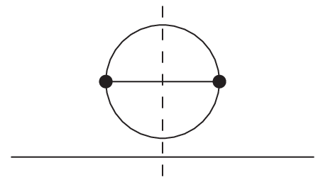
As can be seen in the figure, the spectrum appears to diverge as $c\rightarrow 0$ . This can be understood Polchinski by considering the simplest contribution to the vacuum energy, from the ‘basketball’ graph in Fig. 6.

The zero-mode contribution of this graph to the vacuum energy $E_{0}$ is second order in perturbation theory and can be expressed as

\Delta E\sim\frac{g}{w_{0}^{2}}\frac{1}{E_{0}-4w_{0}/c}\frac{g}{w_{0}^{2}},

(35)

where the middle fraction contains the energy denominator for an intermediate state with four zero-mode bosons and is sandwiched between transition matrix elements for production and annihilation of four zero modes from and to the vacuum. The transition potential is just the first line of ${\cal P}_{+}^{I}$ in (25), which determines the transitions from the vacuum to four bosons and back to the vacuum. The dimensionless individual zero-mode energy is $w_{0}=\tilde{L}\sqrt{c}$ . The shift then diverges as $c^{-3/2}$ , which is consistent with the $c$ dependence shown in Fig. 5.

Clearly, the contributions of vacuum bubbles, such as the contribution represented by the ‘basketball’ graph in Fig. 6, require closer inspection, in order to fully understand the calculation. Recent perturbative analyses Collins; Martinovic of such graphs, comparing light-front and equal-time calculations, also show that some care is required. In fact, the $c\rightarrow 0$ transition can help elucidate the connection between the two quantizations.

III.3 Vacuum bubbles

Following Collins Collins, we first consider the one-loop self-energy in $\phi^{3}$ theory; the graph is given in Fig. 7. The invariant function $\Pi(p^{2})$ is given by

\Pi(p^{2})=-\frac{1}{8\pi^{2}}\int\frac{d^{2}k}{[k^{2}-\mu^{2}+i\epsilon][(p-k)^{2}-\mu^{2}+i\epsilon]}.

(36)

The one-loop bubble is obtained in the $p^{2}\rightarrow 0$ limit, with a value of $\Pi(0)=-i/8\pi\mu^{2}$ .

The covariant graph is, of course, equivalent to two time-ordered graphs, shown in Fig. 8. We then have $\Pi=\Pi_{a}+\Pi_{b}$ with

	$\displaystyle\Pi_{a}(p^{2})$	$\displaystyle=$	$\displaystyle\frac{i}{16\pi}\int\frac{dp_{1-}dp_{2-}}{w_{p_{1}}w_{p_{2}}}\frac{\delta(p_{-}-p_{1-}-p_{2-})}{p_{+}-\sum_{i}^{2}(w_{p_{i}}-sp_{i})/c},$		(37)
	$\displaystyle\Pi_{b}(p^{2})$	$\displaystyle=$	$\displaystyle\frac{i}{16\pi}\int\frac{dp_{1-}dp_{2-}}{w_{p_{1}}w_{p_{2}}}\frac{\delta(p_{-}+p_{1-}+p_{2-})}{p_{+}-2p_{+}-\sum_{i}^{2}(w_{p_{i}}-sp_{i})/c}.$		(38)

These are perturbative quantities, but a nonperturbative calculation in $\phi^{3}$ theory, with the Fock space limited to no more than four constituents, will yield an eigenvalue condition for the light-front energy $P_{+}$ that takes the form

	$\displaystyle P_{+}$	$\displaystyle=$	$\displaystyle\frac{w_{P}-sP_{-}}{c}+\frac{\lambda^{2}}{32\pi}\int\frac{dp_{1-}dp_{2-}}{w_{p_{1}}w_{p_{2}}w_{P}}\frac{\delta(P_{-}-p_{1-}-p_{2-})}{P_{+}-\sum_{i}^{2}\frac{w_{p_{i}}-sp_{i-}}{c}}$		(39)
			$\displaystyle+\frac{\lambda^{2}}{32\pi}\int\frac{dp_{1-}dp_{2-}}{w_{p_{1}}w_{p_{2}}w_{P}}\frac{\delta(P_{-}+p_{1-}+p_{2-})}{P_{+}-2\frac{w_{P}-sP_{-}}{c}-\sum_{i}^{2}\frac{w_{p_{i}}-sp_{i-}}{c}},$		(39)

with an (infinite) two-loop bubble removed. Details are given in the Appendix. The two self-energy terms in (39) correspond to the two time-ordered perturbative graphs.

In the light-front limit $c\rightarrow 0$ , $\Pi_{b}$ makes no contribution, because vacuum vertices do not exist in the light-front limit, and $\Pi_{a}$ becomes, with $p_{2-}=p_{-}-p_{1-}$ , $w_{p_{i}}=p_{i-}$ , and $x\equiv p_{1-}/p_{-}$ ,

\Pi_{a}(p^{2})_{c=0}=\frac{i}{16\pi}\int_{0}^{1}\frac{dx}{x(1-x)}\frac{1}{p^{2}-\frac{\mu^{2}}{2x}-\frac{\mu^{2}}{2(1-x)}}.

(40)

For $p^{2}=0$ , this immediately yields

\Pi_{a}(0)_{c=0}=-\frac{i}{8\pi}\int_{0}^{1}\frac{dx}{\mu^{2}(1-x)+\mu^{2}x}=-\frac{i}{8\pi\mu^{2}}.

(41)

If instead we take $p^{2}=0$ first, we have, with $z\equiv p_{1-}/\sqrt{c}\mu$ , equal contributions from each time-ordered graph

\Pi_{a}(0)=\Pi_{b}(0)=-\frac{i}{16\pi}\int_{-\infty}^{\infty}\frac{c\,dp_{1-}}{(p_{1-}^{2}+c\mu^{2})^{3/2}}=-\frac{i}{16\pi\mu^{2}}\int_{-\infty}^{\infty}\frac{dz}{(1+z^{2})^{3/2}}=-\frac{i}{16\pi\mu^{2}},

(42)

a result independent of $c$ . The sum of the two then replicates the full value of $-i/8\pi\mu^{2}$ .

It is the latter result that is most important for our calculations, because we calculate with finite $c$ and take the zero limit last. Although the analytic integral is independent of $c$ , the numerical approximation associated with taking periodic boundary conditions in a fixed box size is not independent. A small box forces the momentum-space quadrature points to be widely spaced. As $c$ approaches zero, the integrand becomes more sharply peaked in $p_{1-}$ , and the important range of integration is not sampled enough, unless the box is kept sufficiently large. Thus, as $c$ is decreased, the box size must be increased such that $c\tilde{L}^{2}$ is at least of order 1, and the $c\rightarrow 0$ limit does not recover DLCQ, which requires a fixed light-front box size. Instead, the $c\rightarrow 0$ limit must be associated with the continuum limit, where the box is removed.

To illustrate the convergence that can be obtained by taking the continuum limit of $\tilde{L}\rightarrow\infty$ , we consider the numerical estimate of the rescaled quantity

\widetilde{\Pi}_{a}(0)\equiv 16\pi i\mu^{2}\Pi_{a}(0)=\int_{-\infty}^{\infty}\frac{c\mu^{2}\,dp_{1-}}{(w_{p_{1-}})^{3/2}}\simeq\frac{1}{2}c\tilde{L}^{2}\sum_{n=-N}^{N}\frac{1}{(n^{2}+c\tilde{L}^{2})^{3/2}},

(43)

which has the nominal value of 1. However, for the numerical calculation we work at an energy cutoff that determines the range $N$ of the finite sum over the $p_{-}$ index $n$ . For the intermediate Fock state of the one-loop bubble where two constituents have the most energy, the momentum indices are $N$ and $-N$ . The energy limit is then expressed as

E_{\rm max}\geq\frac{\mu}{\tilde{L}}\sum_{n}\frac{\sqrt{n^{2}+c\tilde{L}^{2}}}{c}\rightarrow 2\frac{\mu}{\tilde{L}}\frac{\sqrt{N^{2}+c\tilde{L}^{2}}}{c}.

(44)

This leaves

N\leq\sqrt{c}\tilde{L}\sqrt{\left(\frac{\sqrt{c}E_{\rm max}}{2\mu}\right)^{2}-1}.

(45)

Table 1 shows results for selected values of $c$ and ranges of box size $\tilde{L}$ , with $E_{\rm max}$ varied as needed to keep the same number of quadrature points for different values of $c$ . The cutoff in energy does shift the value away from the nominal value of 1.

Table 1: One-loop and three-loop vacuum bubbles as functions of the dimensionless box size

\tilde{L}\equiv\mu L/\pi

. The energy cutoff

E_{\rm max}

and particular values of

\tilde{L}

are chosen to make the calculation equivalent for each value of the coordinate parameter

c

. The values of

N

indicate the range of discrete steps in momentum, as determined by the energy cutoff. In both cases, the value of

\widetilde{\Pi}_{a}(0)

is independent of

c

and converges in the continuum limit of

\tilde{L}\rightarrow\infty

$c$	1.0000	0.5000	0.2500	0.1250	0.0625	one-loop		three-loop
$E_{\rm max}/\mu$	20.0000	28.2843	40.0000	56.5685	80.0000	$N$	$\widetilde{\Pi}_{a}(0)$	$N$	$\widetilde{\Pi}_{a}(0)$
$\tilde{L}$	1.0000	1.4142	2.0000	2.8284	4.0000	9	1.00696	9	7.03843
$\cdot$	2.0000	2.8284	4.0000	5.6569	8.0000	19	0.99482	19	7.02181
$\cdot$	3.0000	4.2426	6.0000	8.4853	12.0000	29	0.99487	29	7.01538
$\cdot$	4.0000	5.6569	8.0000	11.3137	16.0000	39	0.99491	38	7.01133
$\cdot$	5.0000	7.0711	10.0000	14.1421	20.0000	49	0.99494	48	7.01264
$\cdot$	6.0000	8.4853	12.0000	16.9706	24.0000	59	0.99495	58	7.01426
$\cdot$	7.0000	9.8995	14.0000	19.7990	28.0000	69	0.99497	68	7.01386
$\cdot$	8.0000	11.3137	16.0000	22.6274	32.0000	79	0.99498	77	7.01365
$\cdot$	9.0000	12.7279	18.0000	25.4558	36.0000	89	0.99498	87	7.01381
$\tilde{L}$	10.0000	14.1421	20.0000	28.2843	40.0000	99	0.99499	97	7.01346

The analogous calculation for the three-loop graph in Fig. 6 can also be done numerically. The energy cutoff now limits the range of indices for the four intermediate constituents. Again there are two time orderings, with contributions

\widetilde{\Pi}_{a}(0)=\widetilde{\Pi}_{b}(0)=c\mu^{2}\int\frac{\prod_{i}^{4}dp_{i-}\delta(\sum_{i}^{4}p_{i-})}{(\prod_{i}^{4}w_{p_{i-}})(\sum_{i}^{4}w_{p_{i-}})}.

(46)

The numerical approximation suffers from the same limitations as in the one-loop case, which is why the calculation of the spectrum at fixed box size in Sec. III.2 yields the divergent behavior in Fig. 5. The approximation is

\widetilde{\Pi}_{a}(0)=\widetilde{\Pi}_{b}(0)\simeq c\tilde{L}^{2}\sum_{n_{1},n_{2},n_{3}}^{\rm cutoff}\frac{1}{\left(\prod_{i}^{4}\sqrt{n_{i}^{2}+c\tilde{L}^{2}}\right)\left(\sum_{i}^{4}\sqrt{n_{i}^{2}+c\tilde{L}^{2}}\right)},

(47)

with $n_{4}=-(n_{1}+n_{2}+n_{3})$ and the cutoff specified by

\frac{\mu}{\tilde{L}}\sum_{i}^{4}\frac{w_{n_{i}}-sn_{i}}{c}\leq E_{\rm max}.

(48)

One index is at its maximum $N$ when the other three are all equal to $-N/3$ . This gives $N$ as

N\leq\sqrt{c}\tilde{L}\sqrt{\left(\frac{\sqrt{c}E_{\rm max}}{2\mu}\right)^{2}+4\left(\frac{2\mu}{\sqrt{c}E_{\rm max}}\right)^{2}-5}.

(49)

Values for this numerical approximation are tabulated in Table 1. The convergence with respect to box size is quite rapid.

III.4 Varied box size

The three-loop vacuum bubble is embedded within the full eigenvalue problem for the $\phi^{4}$ vacuum state. Here we consider the vacuum, in both the even and odd sectors, extrapolated in box size. Because the box size is varied, we must consider the vacuum energy density $E/2L$ , rather than the (infinite) vacuum energy. To do this, we compute the lowest eigenvalue of $\frac{1}{2L}{\cal P}_{+}$ , with ${\cal P}_{+}={\cal P}_{+}^{0}+{\cal P}_{+}^{I}$ specified by (14) and (25).

The precise forms of the Hamiltonian terms are

\frac{1}{2L}{\cal P}_{+}^{0}=\frac{\mu^{2}}{2\pi}\sum_{n=-\infty}^{\infty}\frac{w_{n}-sn}{c\tilde{L}^{2}}a^{\dagger}_{n}a_{n},

(50)

	$\displaystyle\frac{1}{2L}{\cal P}_{+}^{I}=\frac{g\mu^{2}}{8\pi}\sum_{n_{1}\ldots n_{4}}\frac{1}{\sqrt{w_{n_{1}}\cdots w_{n_{4}}}}\left[\frac{1}{12}(a_{n_{1}}\cdots a_{n_{4}}+a^{\dagger}_{n_{1}}\cdots a^{\dagger}_{n_{4}})\delta_{n_{1}+\cdots+n_{4},0}\right.$		(51)
	$\displaystyle+\frac{1}{3}(a^{\dagger}_{n_{1}}a_{n_{2}}a_{n_{3}}a_{n_{4}}+a^{\dagger}_{n_{2}}a^{\dagger}_{n_{3}}a^{\dagger}_{n_{4}}a_{n_{1}})\delta_{n_{1},n_{2}+n_{3}+n_{4}}$
	$\displaystyle\left.+\frac{1}{2}a^{\dagger}_{n_{1}}a^{\dagger}_{n_{2}}a_{n_{3}}a_{n_{4}}\delta_{n_{1}+n_{2},n_{3}+n_{4}}\right],$

with $w_{n}=\sqrt{n^{2}+c\tilde{L}^{2}}$ . In these we see that $c$ and $\tilde{L}$ appear only in the combination $c\tilde{L}^{2}$ . Thus, for any positive value of $c$ , a rescaling of the box size makes the calculation equivalent to an equal-time calculation at $c=1$ , with a smaller box. In the limit of infinite box size, the calculation becomes completely independent of $c$ , making the vacuum energy density independent of $c$ , even as $c$ approaches the light-front limit of zero.

For a numerical calculation, there is, of course, an energy cutoff $E_{\rm max}$ . For calculations with different values of $c$ , this cutoff must be adjusted to make the basis sizes equivalent. In a Fock sector with $n$ constituents, the momentum indices lie between $\pm N$ with

N=\sqrt{c}\tilde{L}\sqrt{\left(\frac{\sqrt{c}E_{\rm max}}{2\mu}\right)^{2}+\left(\frac{(n-1)^{2}-1}{4}\right)^{2}\left(\frac{2\mu}{\sqrt{c}E_{\rm max}}\right)^{2}-\frac{(n-1)^{2}+1}{2}}.

(52)

This is determined by giving one constituent $N$ units of momentum and each of the others $-N/(n-1)$ units, to minimize the total Fock-state energy

\frac{\mu}{\tilde{L}}\sum_{n}\frac{w_{n}-sn}{c}=\frac{\mu}{\tilde{L}}\left[\frac{\sqrt{N^{2}+c\tilde{L}^{2}}}{c}+\frac{(n-1)}{c}\sqrt{\frac{N^{2}}{(n-1)^{2}}+c\tilde{L}^{2}}\right].

(53)

From (52) we see that, for fixed $N$ , the energy cutoff must scale as $\mu/\sqrt{c}$ , which is not surprising, given that zero-mode energies diverge as $\mu/\sqrt{c}$ .

For fixed $\sqrt{c}E_{\rm max}$ , the size of the calculation saturates, with $N$ forced to be zero in the highest Fock sectors. Setting $N=0$ and $n=K$ in (52), we find that this occurs at a maximum number $K$ of constituents, given by

K=1\mp 2\pm\sqrt{8-2(1-2\sqrt{c}E_{\rm max}/\mu)}.

(54)

For $E_{\rm max}=20\mu$ and $c=1$ , this limits $K$ to 8 (9) in the even (odd) sector. Beyond these values of $K$ , only zero modes contribute.

With calculations at arbitrary $c$ now shown to be completely equivalent to equal-time calculations, the light-front limit must then reproduce the results found for equal-time quantization RychkovVitale; Rychkov. In particular, they must agree on the value of the critical coupling.

IV Summary

By considering the coordinate interpolation (1), we have been able to study the approach to light-front quantization ( $c=0$ ) from equal-time quantization ( $c=1$ ) in two-dimensional $\phi^{4}$ theory. A numerical calculation of the spectrum, for arbitrary $c>0$ and fixed box size, provides results consistent with those of equal-time quantization RychkovVitale; Rychkov, as shown in Fig. 4. However, the spectrum is found to diverge as $c$ approaches the light-front limit of zero, if the box size is held fixed; see Fig. 5. Although this might be taken as an indication that the light-front limit is not smooth, we have shown that the divergence is instead spurious and caused by a poor numerical representation of vacuum-bubble contributions. The spurious divergence is due to the fixed box size, which prevents the momentum-space grid from being fine enough to sample the vacuum-bubble integrals accurately.

Our nonperturbative analysis of vacuum-bubble contributions replicates the perturbative analysis of Collins Collins. The contributions of the two time-ordered graphs of Fig. 8 are shown to be different, depending on the order of the limits $c\rightarrow 0$ and $p^{2}\rightarrow 0$ ; the sum, however, is invariant. The numerical approximation to these contributions is then shown to be very sensitive to box size. In particular, the $c\rightarrow 0$ limit requires that the continuum limit in momentum space (infinite box size) must be taken as $c\rightarrow 0$ . The DLCQ PauliBrodsky formulation of light-front quantization, with its finite box, will require a different approach for the inclusion of vacuum-bubble contributions.

The vacuum energy density is shown in Sec. III.4 to be independent of $c$ in the continuum limit of infinite box size. This makes a calculation for any $c>0$ explicitly equivalent to an equal-time calculation at $c=1$ . Assuming that the $c\rightarrow 0$ limit is smooth, the light-front spectrum must be nonperturbatively equivalent to the equal-time spectrum, provided vacuum-bubble contributions are taken into account properly. Thus, the apparent disagreement over the value of the critical coupling, resolved by noting differences in mass renormalization BCH, is actually a sign that vacuum effects are not included properly. How to include vacuum bubbles in a native, nonperturbative light-front calculation remains an open question.

Acknowledgements.

This work was supported in part by the Minnesota Supercomputing Institute through grants of computing time and benefited from participation in the workshop on Hamiltonian methods in strongly coupled quantum field theory supported by the Simons Collaboration on the Nonperturbative Bootstrap.

Appendix A Nonperturbative one-loop bubble from $\phi^{3}$ theory

Contributions to the energy that correspond to the time-ordered loops in Fig. 8 arise naturally in a truncated nonperturbative calculation, which we show here. The interaction Hamiltonian for $\phi^{3}$ theory is

{\cal P}_{+}^{I}=\int_{-\infty}^{\infty}dx^{-}\frac{\lambda}{3!}:\phi^{3}:.

(55)

Substitution of the mode expansion (9) and integration over $x^{-}$ yields

$\displaystyle{\cal P}_{+}^{I}$	$\displaystyle=$	$\displaystyle\frac{\lambda}{4\sqrt{4\pi}}\int\frac{dp_{1-}dp_{2-}dp_{3-}}{\sqrt{w_{p_{1}}w_{p_{2}}w_{p_{3}}}}\left\{a^{\dagger}(p_{1-})a(p_{2-})a(p_{3-})\delta(p_{1-}-p_{2-}-p_{3-})\right.$	(56)
		$\displaystyle+a^{\dagger}(p_{1-})a^{\dagger}(p_{2-})a(p_{3-})\delta(p_{1-}+p_{2-}-p_{3-})$
		$\displaystyle\left.+\frac{1}{3}[a(p_{1-})a(p_{2-})a(p_{3-})+a^{\dagger}(p_{1-})a^{\dagger}(p_{2-})a^{\dagger}(p_{3-})]\delta(p_{1-}+p_{2-}+p_{3-})\right\}.$

The eigenstate is expanded in a Fock basis as

$\displaystyle\|\psi(P_{-})\rangle=\psi_{1}a^{\dagger}(P_{-})\|0\rangle+\int dp_{1-}dp_{2-}\delta(P_{-}-p_{1-}-p_{2-})\psi_{2}(p_{1-},p_{2-})\frac{1}{\sqrt{2}}a^{\dagger}(p_{1-})a^{\dagger}(p_{2-})\|0\rangle$		(57)
	$\displaystyle+\int dp_{1-}dp_{2-}dp_{3-}\delta(P_{-}-p_{1-}-p_{2-}-p_{3-})\psi_{3}(p_{1-},p_{2-},p_{3-})\frac{1}{\sqrt{6}}a^{\dagger}(p_{1-})a^{\dagger}(p_{2-})a^{\dagger}(p_{3-})\|0\rangle$
	$\displaystyle+\int dp_{1-}dp_{2-}dp_{3-}dp_{4-}\delta(P_{-}-p_{1-}-p_{2-}-p_{3-}-p_{4-})\psi_{4}(p_{1-},p_{2-},p_{3-},p_{4-})$
	$\displaystyle\hskip 36.135pt\times\frac{1}{\sqrt{24}}a^{\dagger}(p_{1-})a^{\dagger}(p_{2-})a^{\dagger}(p_{3-})a^{\dagger}(p_{4-})\|0\rangle,$

with truncation at four constituents. The action of the free part of the Hamiltonian is

$\displaystyle{\cal P}_{+}^{0}\|\psi(P_{-})\rangle=\frac{w_{P}-sP_{-}}{c}\psi_{1}a^{\dagger}(P_{-})\|0\rangle$		(58)
	$\displaystyle+\int dp_{1-}dp_{2-}\delta(P_{-}-p_{1-}-p_{2-})\sum_{i}^{2}\left[\frac{w_{p_{i}}-sp_{i-}}{c}\right]\psi_{2}(p_{1-},p_{2-})\frac{1}{\sqrt{2}}a^{\dagger}(p_{1-})a^{\dagger}(p_{2-})\|0\rangle$
	$\displaystyle+\int dp_{1-}dp_{2-}dp_{3-}\delta(P_{-}-p_{1-}-p_{2-}-p_{3-})$
	$\displaystyle\hskip 36.135pt\times\sum_{i}^{3}\left[\frac{w_{p_{i}}-sp_{i-}}{c}\right]\psi_{3}(p_{1-},p_{2-},p_{3-})\frac{1}{\sqrt{6}}a^{\dagger}(p_{1-})a^{\dagger}(p_{2-})a^{\dagger}(p_{3-})\|0\rangle$
	$\displaystyle+\int dp_{1-}dp_{2-}dp_{3-}dp_{4-}\delta(P_{-}-p_{1-}-p_{2-}-p_{3-}-p_{4-})$
	$\displaystyle\hskip 36.135pt\times\sum_{i}^{4}\left[\frac{w_{p_{i}}-sp_{i-}}{c}\right]\psi_{4}(p_{1-},p_{2-},p_{3-},p_{4-})\frac{1}{\sqrt{24}}a^{\dagger}(p_{1-})a^{\dagger}(p_{2-})a^{\dagger}(p_{3-})a^{\dagger}(p_{4-})\|0\rangle$

and that of the interaction part, truncated at four constituents, is

$\displaystyle{\cal P}_{+}^{I}\|\psi(P_{-})\rangle$	$\displaystyle=$	$\displaystyle\frac{\lambda}{4\sqrt{4\pi}}\left\{\int\frac{dp_{1-}dp_{2-}}{\sqrt{w_{p_{1}}w_{p_{2}}w_{P}}}\delta(p_{1-}+p_{2-}-P_{-})\psi_{1}a^{\dagger}(p_{1-})a^{\dagger}(p_{2-})\|0\rangle\right.$	(59)
		$\displaystyle+\frac{1}{3}\int\frac{dp_{1-}dp_{2-}dp_{3-}}{\sqrt{w_{p_{1}}w_{p_{2}}w_{p_{3}}}}\delta(p_{1-}+p_{2-}+p_{3-})\psi_{1}a^{\dagger}(p_{1-})a^{\dagger}(p_{2-})a^{\dagger}(p_{3-})a^{\dagger}(P_{-})\|0\rangle$
		$\displaystyle+\sqrt{2}\int\frac{dp_{1-}dp_{2-}}{\sqrt{w_{p_{1}}w_{p_{2}}w_{P}}}\delta(p_{1-}+p_{2-}-P_{-})\psi_{2}(p_{1-},p_{2-})a^{\dagger}(P_{-})\|0\rangle$
		$\displaystyle+\sqrt{2}\int\frac{dp_{1-}dp_{2-}dp_{3-}}{\sqrt{w_{p_{1}}w_{p_{2}}w_{p_{1}+p_{2}}}}\delta(p_{1-}+p_{2-}+p_{3-}-P_{-})$
		$\displaystyle\hskip 36.135pt\times\psi_{2}(p_{1-}+p_{2-},p_{3-})a^{\dagger}(p_{1-})a^{\dagger}(p_{2-})a^{\dagger}(p_{3-})\|0\rangle$
		$\displaystyle+\sqrt{6}\int\frac{dp_{1-}dp_{2-}dp_{3-}}{\sqrt{w_{p_{1}}w_{p_{2}}w_{p_{1}-p_{2}}}}\delta(p_{1-}+p_{3-}-P_{-})$
		$\displaystyle\hskip 36.135pt\times\psi_{3}(p_{1-}-p_{2-},p_{2-},p_{3-})a^{\dagger}(p_{1-})a^{\dagger}(p_{3-})\|0\rangle$
		$\displaystyle+\sqrt{\frac{3}{2}}\int\frac{dp_{1-}dp_{2-}dp_{3-}dp_{4-}}{\sqrt{w_{p_{1}}w_{p_{2}}w_{p_{1}+p_{2}}}}\delta(p_{1-}+p_{2-}+p_{3-}+p_{4-}-P_{-})$
		$\displaystyle\hskip 36.135pt\times\psi_{3}(p_{1-}+p_{2-},p_{3-},p_{4-})a^{\dagger}(p_{1-})a^{\dagger}(p_{2-})a^{\dagger}(p_{3-})a^{\dagger}(p_{4-})\|0\rangle$
		$\displaystyle+\sqrt{\frac{8}{3}}\int\frac{dp_{1-}dp_{2-}dp_{3-}}{\sqrt{w_{p_{1}}w_{p_{2}}w_{p_{3}}}}\delta(p_{1-}+p_{2-}+p_{3-})\psi_{4}(p_{1-},p_{2-},p_{3-},P_{-})a^{\dagger}(P_{-})\|0\rangle$
		$\displaystyle+\sqrt{6}\int\frac{dp_{1-}dp_{2-}dp_{3-}dp^{\prime}_{1-}}{\sqrt{w_{p_{1}}w_{p^{\prime}_{1}}w_{p_{1}-p^{\prime}_{1}}}}\delta(p_{1-}+p_{2-}+p_{3-}-P_{-})$
		$\displaystyle\hskip 36.135pt\left.\times\psi_{4}(p^{\prime}_{1-},p_{1-}-p^{\prime}_{1-},p_{2-},p_{3-})a^{\dagger}(p_{1-})a^{\dagger}(p_{2-})a^{\dagger}(p_{3-})\|0\rangle\right\}.$

From these contributions, we can construct the eigenvalue problem ${\cal P}_{+}|\psi(P_{-})\rangle=P_{+}|\psi(p_{-})\rangle$ as projections onto different Fock sectors. These projections are

	$\displaystyle\frac{w_{P}-sP_{-}}{c}\psi_{1}+\sqrt{2}\frac{\lambda}{4\sqrt{4\pi}}\int\frac{dp_{1-}dp_{2-}}{\sqrt{w_{P}w_{p_{1}}w_{p_{2}}}}\delta(P_{-}-p_{1-}-p_{2-})\psi_{2}(p_{1-},p_{2-})$						(60)
			$\displaystyle+\sqrt{\frac{8}{3}}\frac{\lambda}{4\sqrt{4\pi}}\int\frac{dp_{1-}dp_{2-}dp_{3-}}{\sqrt{w_{p_{1}}w_{p_{2}}w_{p_{3}}}}\delta(p_{1-}+p_{2-}+p_{3-})\psi_{4}(p_{1-},p_{2-},p_{3-},P_{-})=P_{+}\psi_{1},$				(60)

	$\displaystyle\sum_{i}^{2}\frac{w_{p_{i}}-sp_{i-}}{c}\psi_{2}(p_{1-},p_{2-})+\frac{\lambda}{4\sqrt{4\pi}}\frac{\sqrt{2}\psi_{1}}{\sqrt{w_{p_{1}}w_{p_{2}}w_{P}}}$						(61)
			$\displaystyle+\sqrt{12}\frac{\lambda}{4\sqrt{4\pi}}\int\frac{dp^{\prime}_{2-}}{\sqrt{w_{p_{1}}w_{p^{\prime}_{2}}w_{p_{1}-p^{\prime}_{2}}}}\psi_{3}(p_{1-}-p^{\prime}_{2-},p^{\prime}_{2-},p_{2-})=P_{+}\psi_{2},$				(61)

	$\displaystyle\sum_{i}^{3}\frac{w_{p_{i}}-sp_{i-}}{c}\psi_{3}(p_{1-},p_{2-},p_{3-})+\frac{\lambda}{4\sqrt{4\pi}}\frac{\sqrt{12}\psi_{2}(p_{1-}+p_{2-},p_{3-})}{\sqrt{w_{p_{1}}w_{p_{2}}w_{p_{1}+p_{2}}}}$						(62)
			$\displaystyle+6\frac{\lambda}{4\sqrt{4\pi}}\int\frac{dp^{\prime}_{1-}}{\sqrt{w_{p_{1}}w_{p^{\prime}_{1}}w_{p_{1}-p^{\prime}_{1}}}}\psi_{4}(p^{\prime}_{1-},p_{1-}-p^{\prime}_{1-},p_{2-},p_{3-})=P_{+}\psi_{3},$				(62)

$\displaystyle\sum_{i}^{4}\frac{w_{p_{i}}-sp_{i-}}{c}\psi_{4}(p_{1-},p_{2-},p_{3-},p_{4-})+\frac{\lambda}{4\sqrt{4\pi}}\frac{6\psi_{3}(p_{1-}+p_{2-},p_{3-},p_{4-}}{\sqrt{w_{p_{1}}w_{p_{2}}w_{p_{1}+p_{2}}}}$		(63)
	$\displaystyle+\frac{\lambda}{4\sqrt{4\pi}}\frac{\psi_{1}}{\sqrt{6}}\left[\frac{\delta(p_{1-}+p_{2-}+p_{3-})}{\sqrt{w_{p_{1}}w_{p_{2}}w_{p_{3}}}}+\frac{\delta(p_{1-}+p_{3-}+p_{4-})}{\sqrt{w_{p_{1}}w_{p_{3}}w_{p_{4}}}}\right.$
	$\displaystyle\left.\hskip 72.26999pt+\frac{\delta(p_{1-}+p_{2-}+p_{4-})}{\sqrt{w_{p_{1}}w_{p_{2}}w_{p_{4}}}}+\frac{\delta(p_{2-}+p_{3-}+p_{4-})}{\sqrt{w_{p_{2}}w_{p_{3}}w_{p_{4}}}}\right]=P_{+}\psi_{4}.$

We next invert the equations (61) and (63) for $\psi_{2}$ and $\psi_{4}$ , neglecting the higher-order corrections that come from the $\psi_{3}$ -contributions determined by (62), and substitute into the equation (60) for $\psi_{1}$ . This leaves a single implicit equation for $P_{+}$ , with $\psi_{1}$ as a common factor, which we remove. After some simplications that combine algebraic factors and that integrate over all but one delta function, we obtain

$\displaystyle P_{+}$	$\displaystyle=$	$\displaystyle\frac{w_{P}-sP_{-}}{c}+\frac{\lambda^{2}}{32\pi}\int\frac{dp_{1-}dp_{2-}}{w_{p_{1}}w_{p_{2}}w_{P}}\frac{\delta(P_{-}-p_{1-}-p_{2-})}{P_{+}-\sum_{i}^{2}\frac{w_{p_{i}}-2p_{i-}}{c}}$	(64)
		$\displaystyle+\frac{\lambda^{2}}{32\pi}\int\frac{dp_{1-}dp_{2-}}{w_{p_{1}}w_{p_{2}}w_{P}}\frac{\delta(P_{-}+p_{1-}+p_{2-})}{P_{+}-2\frac{w_{P}-sP_{-}}{c}-\sum_{i}^{2}\frac{w_{p_{i}}-2p_{i-}}{c}}$
		$\displaystyle+\frac{1}{3}\delta(0)\frac{\lambda^{2}}{32\pi}\int\frac{dp_{1-}dp_{2-}dp_{3-}}{w_{p_{1}}w_{p_{2}}w_{p_{3}}}\frac{\delta(p_{1-}+p_{2-}+p_{3-})}{P_{+}-\sum_{i}^{3}\frac{w_{p_{i}}-2p_{i-}}{c}-\frac{w_{P}-sP_{-}}{c}}.$

The second and third terms on the right correspond to the time-ordered graphs in Fig. 7. The last term is a disconnected two-loop bubble, which injects an infinite constant to be subtracted; it corresponds to the graph in Fig. 9. The result quoted in (39) is just this equation after subtraction of the two-loop bubble.

References

(1) M. Hogervorst, S. Rychkov and B. C. van Rees, Phys. Rev. D 91, 025005 (2015).
(2) S. Rychkov and L.G. Vitale, Phys. Rev. D 91, 085011 (2015); Phys. Rev. D 93, 065014 (2016).
(3) J. Elias-Miro, M. Montull and M. Riembau, JHEP 1604, 144 (2016); J. Elias-Miro, S. Rychkov and L. G. Vitale, Phys. Rev. D 96, 065024 (2017); JHEP 1710, 213 (2017).
(4) A. Pelissetto and E. Vicari, Phys. Lett. B 751, 532 (2015).
(5) P. Bosetti, B. De Palma and M. Guagnelli, Phys. Rev. D 92, 034509 (2015); B. De Palma and M. Guagnelli, PoS LATTICE 2016, 277 (2016); S. Bronzin, B. De Palma and M. Guagnelli, Phys. Rev. D 99, 034508 (2019).
(6) Z. Bajnok and M. Lajer, JHEP 1610, 050 (2016).
(7) M. Burkardt, S.S. Chabysheva, and J.R. Hiller, Phys. Rev. D 94, 065006 (2016); S.S. Chabysheva and J.R. Hiller, Phys. Rev. D 95, 096016 (2017).
(8) N. Christensen, Comput. Phys. Commun. 222, 167 (2018)
(9) N. Anand, V. X. Genest, E. Katz, Z. U. Khandker and M. T. Walters, JHEP 1708, 056 (2017).
(10) A. L. Fitzpatrick, J. Kaplan, E. Katz, L. G. Vitale and M. T. Walters, JHEP 1808, 120 (2018).
(11) A. L. Fitzpatrick, E. Katz and M. T. Walters, “Nonperturbative Matching Between Equal-Time and Lightcone Quantization,” arXiv:1812.08177 [hep-th].
(12) N. Anand, A. L. Fitzpatrick, E. Katz, Z. U. Khandker, M. T. Walters and Y. Xin, “Introduction to Lightcone Conformal Truncation: QFT Dynamics from CFT Data,” arXiv:2005.13544 [hep-th].
(13) M. Serone, G. Spada, and G. Villadoro, JHEP 1808, 148 (2018); JHEP 1905, 047 (2019); G. Sberveglieri, M. Serone and G. Spada, Phys. Rev. D 100, 045008 (2019).
(14) D. Kadoh, Y. Kuramashi, Y. Nakamura, R. Sakai, S. Takeda, and Y. Yoshimura, JHEP 1905, 184 (2019).
(15) P. Romatschke, JHEP 1903, 149 (2019); Mod. Phys. Lett. A 35, 2050054 (2020).
(16) M. Burkardt, Phys. Rev. D 47, 4628 (1993).
(17) S.J. Brodsky, H.-C. Pauli, and S.S. Pinsky, Phys. Rep. 301, 299 (1998).
(18) M. Burkardt, Adv. Nucl. Phys. 23, 1 (2002).
(19) J.R. Hiller, Prog. Part. Nucl. Phys. 90, 75 (2016).
(20) J. Collins, “The non-triviality of the vacuum in light-front quantization: An elementary treatment,” arXiv:1801.03960 [hep-ph].
(21) L. Martinovic and A. Dorokhov, “Vacuum loops in light-front field theory,” arXiv:1812.02336 [hep-th].
(22) P.D. Mannheim, P. Lowdon and S.J. Brodsky, Phys. Lett. B 797, 134916 (2019); P. D. Mannheim, Phys. Rev. D 102, 025020 (2020); P. D. Mannheim, P. Lowdon and S. J. Brodsky, “Comparing light-front quantization with instant-time quantization,” arXiv:2005.00109 [hep-ph].
(23) K. Hornbostel, Phys. Rev. D 45, 3781 (1992).
(24) Y. Frishman, C.T. Sachrajda, H. Abarbanel, and R. Blankenbecler, Phys. Rev. D 15, 2275 (1977).
(25) D.V. Ahluwalia, in the proceedings of HUGS at CEBAF, edited by W.W. Buck, 1990 (unpublished); D.V. Ahluwalia and D.J. Ernst, Report No. CTP-TAMU 91/90 (unpublished).
(26) M.S. Sawicki, Phys. Rev. D 44, 433 (1991); Phys. Lett. B 268, 327 (1991).
(27) T.W. Chen, Phys. Rev. D 3, 1989 (1971).
(28) E. Elizalde and J. Gomis, Nuovo Cim. A 35, 367 (1976).
(29) E.V. Prokhvatilov and V.A. Franke, Sov. J. Nucl. Phys. 49, 688 (1989).
(30) R. Lenz, M. Thies, S. Levit, and K. Yazaki, Ann. Phys. 208, 1 (1991).
(31) C.-R. Ji and C. Mitchell, Phys. Rev. D 64, 085013 (2001); C.-R. Ji and A. T. Suzuki, Phys. Rev. D 87, 065015 (2013)
(32) S. Weinberg, Phys. Rev. 150, 1313 (1966); S. J. Chang, R. G. Root and T. M. Yan, Phys. Rev. D 7, 1133 (1973); S. J. Chang and T. M. Yan, Phys. Rev. D 7, 1147 (1973); T. M. Yan, Phys. Rev. D 7, 1760 (1973); Phys. Rev. D 7, 1780 (1973).
(33) P.A.M. Dirac, Rev. Mod. Phys. 21, 392 (1949).
(34) H.-C. Pauli and S.J. Brodsky, Phys. Rev. D 32, 1993 (1985); 32, 2001 (1985).
(35) D. G. Robertson, Phys. Rev. D 47, 2549 (1993).
(36) S. S. Pinsky, B. van de Sande, and J. R. Hiller, Phys. Rev. D 51, 726 (1995).
(37) S. S. Chabysheva and J. R. Hiller, Phys. Rev. D 79, 096012 (2009).
(38) S. Hellerman and J. Polchinski, Phys. Rev. D 59, 125002 (1999).

$\displaystyle\|\psi(P_{-})\rangle=\psi_{1}a^{\dagger}(P_{-})\|0\rangle+\int dp_{1-}dp_{2-}\delta(P_{-}-p_{1-}-p_{2-})\psi_{2}(p_{1-},p_{2-})\frac{1}{\sqrt{2}}a^{\dagger}(p_{1-})a^{\dagger}(p_{2-})\|0\rangle$		(57)
	$\displaystyle+\int dp_{1-}dp_{2-}dp_{3-}\delta(P_{-}-p_{1-}-p_{2-}-p_{3-})\psi_{3}(p_{1-},p_{2-},p_{3-})\frac{1}{\sqrt{6}}a^{\dagger}(p_{1-})a^{\dagger}(p_{2-})a^{\dagger}(p_{3-})\|0\rangle$
	$\displaystyle+\int dp_{1-}dp_{2-}dp_{3-}dp_{4-}\delta(P_{-}-p_{1-}-p_{2-}-p_{3-}-p_{4-})\psi_{4}(p_{1-},p_{2-},p_{3-},p_{4-})$
	$\displaystyle\hskip 36.135pt\times\frac{1}{\sqrt{24}}a^{\dagger}(p_{1-})a^{\dagger}(p_{2-})a^{\dagger}(p_{3-})a^{\dagger}(p_{4-})\|0\rangle,$

$\displaystyle{\cal P}_{+}^{0}\|\psi(P_{-})\rangle=\frac{w_{P}-sP_{-}}{c}\psi_{1}a^{\dagger}(P_{-})\|0\rangle$		(58)
	$\displaystyle+\int dp_{1-}dp_{2-}\delta(P_{-}-p_{1-}-p_{2-})\sum_{i}^{2}\left[\frac{w_{p_{i}}-sp_{i-}}{c}\right]\psi_{2}(p_{1-},p_{2-})\frac{1}{\sqrt{2}}a^{\dagger}(p_{1-})a^{\dagger}(p_{2-})\|0\rangle$
	$\displaystyle+\int dp_{1-}dp_{2-}dp_{3-}\delta(P_{-}-p_{1-}-p_{2-}-p_{3-})$
	$\displaystyle\hskip 36.135pt\times\sum_{i}^{3}\left[\frac{w_{p_{i}}-sp_{i-}}{c}\right]\psi_{3}(p_{1-},p_{2-},p_{3-})\frac{1}{\sqrt{6}}a^{\dagger}(p_{1-})a^{\dagger}(p_{2-})a^{\dagger}(p_{3-})\|0\rangle$
	$\displaystyle+\int dp_{1-}dp_{2-}dp_{3-}dp_{4-}\delta(P_{-}-p_{1-}-p_{2-}-p_{3-}-p_{4-})$
	$\displaystyle\hskip 36.135pt\times\sum_{i}^{4}\left[\frac{w_{p_{i}}-sp_{i-}}{c}\right]\psi_{4}(p_{1-},p_{2-},p_{3-},p_{4-})\frac{1}{\sqrt{24}}a^{\dagger}(p_{1-})a^{\dagger}(p_{2-})a^{\dagger}(p_{3-})a^{\dagger}(p_{4-})\|0\rangle$

$\displaystyle{\cal P}_{+}^{I}\|\psi(P_{-})\rangle$	$\displaystyle=$	$\displaystyle\frac{\lambda}{4\sqrt{4\pi}}\left\{\int\frac{dp_{1-}dp_{2-}}{\sqrt{w_{p_{1}}w_{p_{2}}w_{P}}}\delta(p_{1-}+p_{2-}-P_{-})\psi_{1}a^{\dagger}(p_{1-})a^{\dagger}(p_{2-})\|0\rangle\right.$	(59)
		$\displaystyle+\frac{1}{3}\int\frac{dp_{1-}dp_{2-}dp_{3-}}{\sqrt{w_{p_{1}}w_{p_{2}}w_{p_{3}}}}\delta(p_{1-}+p_{2-}+p_{3-})\psi_{1}a^{\dagger}(p_{1-})a^{\dagger}(p_{2-})a^{\dagger}(p_{3-})a^{\dagger}(P_{-})\|0\rangle$
		$\displaystyle+\sqrt{2}\int\frac{dp_{1-}dp_{2-}}{\sqrt{w_{p_{1}}w_{p_{2}}w_{P}}}\delta(p_{1-}+p_{2-}-P_{-})\psi_{2}(p_{1-},p_{2-})a^{\dagger}(P_{-})\|0\rangle$
		$\displaystyle+\sqrt{2}\int\frac{dp_{1-}dp_{2-}dp_{3-}}{\sqrt{w_{p_{1}}w_{p_{2}}w_{p_{1}+p_{2}}}}\delta(p_{1-}+p_{2-}+p_{3-}-P_{-})$
		$\displaystyle\hskip 36.135pt\times\psi_{2}(p_{1-}+p_{2-},p_{3-})a^{\dagger}(p_{1-})a^{\dagger}(p_{2-})a^{\dagger}(p_{3-})\|0\rangle$
		$\displaystyle+\sqrt{6}\int\frac{dp_{1-}dp_{2-}dp_{3-}}{\sqrt{w_{p_{1}}w_{p_{2}}w_{p_{1}-p_{2}}}}\delta(p_{1-}+p_{3-}-P_{-})$
		$\displaystyle\hskip 36.135pt\times\psi_{3}(p_{1-}-p_{2-},p_{2-},p_{3-})a^{\dagger}(p_{1-})a^{\dagger}(p_{3-})\|0\rangle$
		$\displaystyle+\sqrt{\frac{3}{2}}\int\frac{dp_{1-}dp_{2-}dp_{3-}dp_{4-}}{\sqrt{w_{p_{1}}w_{p_{2}}w_{p_{1}+p_{2}}}}\delta(p_{1-}+p_{2-}+p_{3-}+p_{4-}-P_{-})$
		$\displaystyle\hskip 36.135pt\times\psi_{3}(p_{1-}+p_{2-},p_{3-},p_{4-})a^{\dagger}(p_{1-})a^{\dagger}(p_{2-})a^{\dagger}(p_{3-})a^{\dagger}(p_{4-})\|0\rangle$
		$\displaystyle+\sqrt{\frac{8}{3}}\int\frac{dp_{1-}dp_{2-}dp_{3-}}{\sqrt{w_{p_{1}}w_{p_{2}}w_{p_{3}}}}\delta(p_{1-}+p_{2-}+p_{3-})\psi_{4}(p_{1-},p_{2-},p_{3-},P_{-})a^{\dagger}(P_{-})\|0\rangle$
		$\displaystyle+\sqrt{6}\int\frac{dp_{1-}dp_{2-}dp_{3-}dp^{\prime}_{1-}}{\sqrt{w_{p_{1}}w_{p^{\prime}_{1}}w_{p_{1}-p^{\prime}_{1}}}}\delta(p_{1-}+p_{2-}+p_{3-}-P_{-})$
		$\displaystyle\hskip 36.135pt\left.\times\psi_{4}(p^{\prime}_{1-},p_{1-}-p^{\prime}_{1-},p_{2-},p_{3-})a^{\dagger}(p_{1-})a^{\dagger}(p_{2-})a^{\dagger}(p_{3-})\|0\rangle\right\}.$


(a)	(b)

Transitioning from equal-time to light-front quantization in ϕ24\phi_{2}^{4} theory