Quantum Brownian motion simulation of the control effect for two harmonic oscillators coupling in position and momentum with general environmentPreprint: APS/123-QED
Abstract
In this paper, we study the dynamical properties of two coupled quantum harmonic oscillators coupled with bosonic non-Markovian environment both in position and momentum. We deduce the exact analytical master equation using Quantum State Diffusion method and give the quantum trajectory description when the control is added to the system by applying interaction between two harmonic oscillators. With numerical simulation, we compare the evolution of entanglement under different controlling effects. At last, we use nonlinear QSD method to strengthen our above results by getting the same evolution.
I Introduction
The study of quantum open systems are increasingly important in the field of quantum dynamics because it is impossible to isolate the system from its environment or make a measurement without involving with other systems. Generally, although environment and specific quantum system are initially independent, they will become entangled due to the interaction, as a result, the quantum system will no longer be pure state which means the evolution operator is non-unitary. Most experimental physicists face the quantum open system where a small system of interest coupled to a large system with a large number of freedom, which can be described by heat bath. Traditionally, we describe the open system by a Lindblad master equation which can be derived with Born-Markov approximation which means the flow of energy or information is unidirectional, in other words, the bath is memoryless. However, if the bath memory effects are relevant, for example in the cases of a high-Q cavity, atom laser or complex structured environment, where the Born-Markov approximation does not work, we have to use Non-Markovian process to describe the quantum system.
Quantum Brownian Motion (QBM) is a paradigm of quantum open system motivated by possible observation of macroscopic effects in quantum systems and problem of quantum measurement theory. Also, Quantum Brownian Motion, as a exactly-solvable model, provides us a glance at the relationship between different measure of quantum systems, including entanglement, coherence, purity, during the evolution of quantum system and under the external time-dependent control. To study the quantum-to-classical transition in quantum cosmology, Hu, Paz and Zhang got the exact master equation with nonlocal dissipation and colored noise in a general environment, which beginning the new stage to treat the old problemHPZ. Iater, Chou, Ting and Hu derived an exact master equation for two coupled quantum harmonic oscillators interacting via bilinear coupling with a common environment at arbitrary temperature made up of many harmonic oscillators with a general spectral density functionyu2ho, which makes it possible to study the decoherence and disentangle in Brownian motion model. Traditionally, we use reduced density matrix to describe the quantum open system when we consider the environment effect to the specific system. Recently, there are tremendous progresses in the development of stochastic Schrodinger equations to describe the quantum open system. We will have the reduced density matrix by tracing over the quantum trajectories of a stochastic Schrodinger equation, which means a possible series of influence of the environment to the system. Quantum state diffusion method provides not only an efficient way in the numerical calculation of quantum open system, but also a way to describe our system, which shed light on the difficulties encountered in environment memory effect.
In this paper, we mainly give the numerical simulation and derivation of the stochastic Schrodinger equation and master equation for open quantum system containing two time-dependent interacting harmonic oscillators, coupled with a thermal bath involving infinite number of bosonic oscillators at zero temperature. The symmetric position-momentum coupling pattern is used, which also can be regarded as a Rotating Wave Approximation of position. We also shows in zero temperature case, the symmetric coupling in position and momentum provides an easy but effective way to have an glance at the quantum system under the influence of environment and external control field, especially for numerical simulations, because ten related differential equations are simplified to one differential equation.
Our paper is organized as follows. We firstly give a brief introduction to Quantum State Diffusion method, in zero temperature in Section II.1. The evolution of two harmonic oscillators with the symmetric coupled pattern in position and momentum in Section II.2 is considered, where the time-local, convolution-less master equation, derived by non-Markovian quantum state diffusion method(NMQSD). We then consider the application of quantum control in Section III.1 where we control the entanglement and coherence of the specific quantum system by time-dependent interaction. In Section III.2, we simulate these controlling and non-Markov process, including coherence states, folk states and cat states under the influence of environment and control field.
II Theoretical Framework
II.1 Introduction to QSD in zero temperature
The standard total Hamiltonian in the system-plus-reservoir in quantum open system can always be written as
| (1) |
where is the system operator providing the coupling between the system and the environment and are coupling constants. we will then set .
Using the Schrodinger equation, the non-Markov Quantum State Diffusion (NMQSD) equation is yu1ho
| (2) |
where is the bath correlation function determinant by temperature and initial bath states, is the system Hamiltonian and are Gaussian random process with correlation functions that mirror the vacuum correlations of the bath operators in the interaction picture.
It is possible to replace the functional derivative by some time-dependent operator , which depends on the time , , and the entire history of the stochastic process . by making an ansatz, the evolution equation for operator is
| (3) |
where the time-integrated operator is the integral of from 0 to t with the weight function
| (4) |
is the correlation function to describe the influence of the environment to the system, which depends on the spectral density of the system and temperature.
| (5) |
Our numerical results focus on zero temperature and finite temperature. We can introduce the spectral density of bath oscillators:
| (6) |
Later we choose super-Ohmic environment in our numerical computation. is a cutoff function, of which is cutoff frequency, the most important parameters to control our environmental spectrum. In our simulation, cutoff function is chosen to be .
The problem of solving stochastic Schrodinger equation is more and less solving operator, exactly or approximately. The general QSD equation can be simplified to a form which may be simulated numerically, as long as the ansatz satisfies the consistency condition. In practice, even when the operator cannot be determined exactly, perturbation techniques may be used to create a serious of operator allowing for an approximate form of general QSD equation. Fortunately, we can find exact for two coupled harmonic oscillators. The convolution-less form of NMQSD equation will appear if we replace the functional derivative by the known operator
| (7) |
Once we have the NMQSD equation, the reduced density operator is given by the ensemble mean over the trajectories of the stochastic Schrodinger equation.
| (8) |
If the exact operator is independent of the noise , we can find that
II.2 Quantum Brownian motion with coupling symmetric in position and momentum by Quantum State Diffusion
Quantum Brownian motion of a damped harmonic oscillator bi linearly coupled to bath of harmonic oscillators has been studied for decades and the non-Markov exact master equation was provided by path integral techniquesyu2ho. This part will provide another approach to exact master equation by Quantum State Diffusion. In the more generalized forms, the masses and frequencies of the oscillators are different so that the master equation can be used easily in the research of non resonant problems. Also, the couple between two harmonic oscillators is a function of time to research the quantum control application, and if we are not interested in the control part we can set .
The Hamiltonian of the total system consisting of a system of two mutually coupled harmonic oscillators with different mass and frequency interacting with a bath of harmonic oscillators of masses and frequencies in an equilibrium state at zero temperature:
| (10) |
where
| (11) |
is the system Hamiltonian for the two system oscillators of interest, with displacements and momentum and time dependent couple function .
| (12) |
is the bath Hamiltonian with displacements and conjugate momentum.
One solvable model is that
the system and the environment are coupled through different observables:
| (13) |
For simplification, we assume the masses and frequencies of those harmonic oscillators are same. It is easy to rewrite this interaction Hamiltonian in creation and annihilation operatorspaz2ho
| (14) |
The same type can also be derived from standard position-position coupling with rotating-wave
approximation (RWA). In the expansion
of , we can rewrite this in terms of creation and annihilation
operators as .
In RWA, high-frequency oscillating terms like and
are neglected. If we rewrite the system with RWA interaction as:
| (15) |
In this model, the Lindblad operator will be . We find the operator without an explicit noise dependence:
| (16) |
Define the integration of function with the correlation function as weight function
| (17) |
The complex function f follows the evolution equation and boundary condition:
| (18) |
| (19) |
We can get the analytical solution if the frequency distribution is Lorentz spectrum, where .If we integral both sides of the evolution equation of from to with , we will have
| (20) |
which is Riccati Equation. Solve the equation with transformation
and we will have
| (21) |
Finally, the solution is
| (22) |
where the parameters determines whether is complex or real. In this case, as long as or , the system will be non-Markov.
After obtaining the evolution of , master equation turns to be as follows:
| (23) |

Markov when time goes by.

non-Markov properties.
and have been chosen to be 1 for simplicity. It is remarkable that this case is only for zero temperature where the Landblad operator is not Hermitian, . It is a good example to solve numerically because eight related integral-diffential equations have been reduced to only one integral-diffential equation .
The resulting nonlinear, convolution less non-Markov stochastic Schrodinger
equation for the Brownian motion of a harmonic oscillator with a coupling
to the environment through position thus reads
| (24) |
Here, we have the notation
| (25) |
and the noise term
| (26) |
III Application in Quantum Control
In this section, we present theoretical analysis and numerical results of the open quantum system.
III.1 Quantum control for entanglement for gaussian states
The decoherence of two harmonic oscillators has been studied systematically in yu2ho; paz2ho where coupling constant between two oscillators is constant. If we control the coupling relation as a function of time, we can control the decoherence. With the control function, we can transform the dynamical phase from one to a different one. or simplification, we assume the masses and frequencies of those harmonic oscillators are same (resonant case).
It is convenient to use coordinates since couples to the environment while is controlled:
| (27) |
The system is simplified to a harmonic oscillator coupled to environment and another harmonic oscillator controlled by external time dependent frequency . The master equation for one harmonic oscillatorHPZ is
| (28) |
where the renormalized Hamiltonian is
| (29) |
where the coefficients depend on the spectral density of the environment. The second moments of and according to paz2ho are
| (30) |
| (31) |
Then, the system will become two separable harmonic oscillators: one is coupled with environment and another one is under the control. Similarly, we can have the second moments for and .
| (32) |
| (33) |
We assume that the initial state of system is Gaussian. Because the complete evolution is linear and all the operators are quadratic, the Gaussian nature of the state will be preserved for all times. The entanglement for Gaussian states is entirely determined by the properties of the con-variance matrix. The covariance matrix (CM) is a real symmetric and positive matrix.
| (34) |
where the matrix elements are defined as:
| (35) |
where . CM also has the structure
| (36) |
where and are Hermitian matrices and denotes the transposed matrix. and denote the symmetric covariance matrices for the individual reduced one-mode states, while the matrix contains the cross-correlations between modes. The advantage of gaussian state is that a good measure of entanglement for such states is logarithmic negativity , which can be computed as
| (37) |
where is the smallest symplectic eigenvalue of the partially transposed covariance matrix.Some expressions for based on previous paper paz2ho have been known. For two mode squeezed state, obtained from the vacuum by acting with the creation operator , we would have . For this squeezed state, the dispersions satisfy the minimum uncertainty condition . The squeezing factor determines the ratio between variances since . If , the state becomes localized in the and variables approaching an ideal Einstein-Podolsky-Rosen state. We will use numerical simulation to see how time-dependent control external field will influence the evolution of entanglement.
III.2 Numerical results and discussion
Within the framework of evolution equation, entanglement, system energy and quantum coherence, measured by norm can be investigated numerically. Initially, we consider the simplest case, the symmetric coupling between momentum and position in zero temperature, to show how input control can result in the change of entanglement, energy and coherence. We keep the parameters of environment, which is strong non-Markov case, and the coupling between two harmonic oscillators weak relative to coupling between system and environment. We simulate system by evolute the master equation. The initial states for all simulations are squeezed states created by squeezed operator , we would have . Without control, the entanglement, coherence and energy will decrease from the initial value with fluctuations, where the non-Markov environment results in fluctuation by information and energy back flow. In long time limit, the entanglement will stay in a stable value.
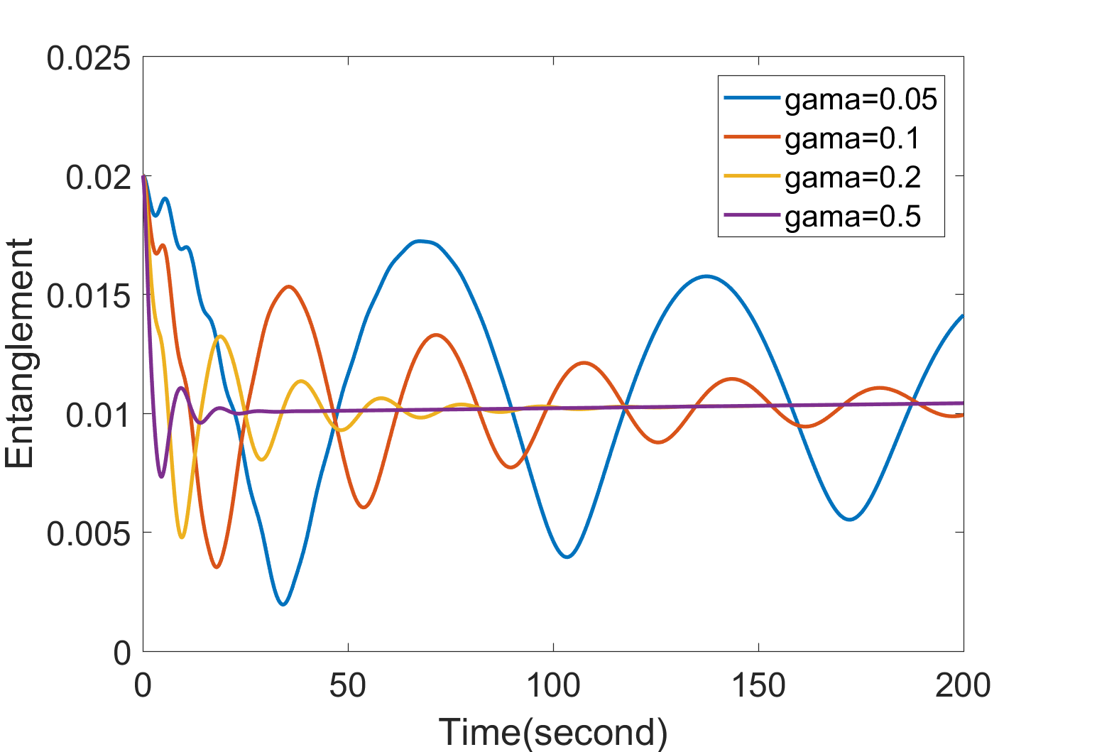
With the control which frequency is much greater than the response frequency, the entanglement will decrease with oscillations with high input frequency but get stable value more quickly, which means high-frequency input cannot influence the entanglement to reach a new point which does not exist before the control. There are several resonance frequencies as shown in the figure. Keeping the strength of the input signal but changing the frequency, the oscillation of the entanglement, energy and coherence is growing while the frequency is approaching to the resonance frequency, and decaying while the frequency is leaving the resonance frequency. When the input signal frequency is exactly same as the resonance frequency, the energy will accumulate to a high level compared with non-resonance cases and fluctuate, as what happens in classical regime, and the analysis of classical system with comparison between classical system and quantum system will be given later. The coherence will increase with similar trend as energy which can be regarded as the input of information with energy, then the flowing of information and energy to environment is weakened by changing to a specific resonance frequency compared to the incoming flowing information and energy, which results in the accumulation of energy and information.There is an interesting phenomenon for entanglement in the resonance cases, after reaching the highest point, the entanglement drops quickly with fluctuation and reaches zero, which means two harmonic oscillators disentangle just after the maximum of entanglement. The entanglement between two harmonic oscillators cannot reach zero because the environment is non-markov except by resonance control, which is different from classical cases. In experiment, the input signal with specific frequency can protect the system coherence and entanglement from real environment.


In order to make our results more credible, we calculate two above-mentioned models using two different methods, one by quantum state diffusion equation and the other by master equation. If our above results are valid, these two methods should give the same evolutionary picture of entanglement over time. Finally, our comparation clearly shows when the number of trajectories run by equation of quantum state diffusion is large enough, it gives the highly likely result with master equation, which shows our above numerical discussion is believable enough.


IV Conclusion
In this paper, we studied the control effect with two interacting
oscillators coupled with bosonic thermal bath by the method of quantum brownian motion. Non-Markovian master
equation of reduced density matrix is obtained by quantum state diffusion
method and one momentum-position coupling patterns are considered. There are
several attracting questions remaining in this work. We noticed that
after interacting with environment, two quantum oscillators evolve
from a pure state to a final mixed state, and correspondingly physical
quantities such as energy of system, quantum coherence and purity
remain at a non-zero level after fluctuating at the beginning. Environment
has the ability to build up coherence and entanglement but cannot
totally destroy the connection or squeeze all information contained
within system back to surroundings. Classically second law of thermodynamics
might help us to understand relative phenomenon in qualitative view
but we aim to find out the quantitative interpretation by means of
this model. We speculate that there could be some symmetry protected
process which makes the system get rid of thorough destruction in
long-time limit. Relevant investigation will be presented in future
work.
References
- [1] Juan Pablo Paz B .L Hu and Yuhong Zhang. Quantum brownian motion in a general enviornment: Exact master equation with nonlocal dissipation and colored noise. Phys. Rev. D, 1992.
- [2] Ting Yu Chung-Hsien Chou and B. L. Hu. Exact master equation and quantum decoherence of two coupled harmonic oscillators in a general environment. Phys. Rev. E, 2008.
- [3] Juan Pablo Paz, Juan Pablo and Augusto J. Roncaglia. Dynamical phases for the evolution of the entanglement between two oscillators coupled to the same environment. Phys. Rev. A, 2009.
- [4] Walter T. Strunz and Ting Yu. Convolutionless non-markovian master equations and quantum trajectories: Brown motion. Phys. Rev. A, 95(4), 2004.