Estimating the Signal Reconstruction Error from Threshold-Based Sampling Without Knowing the Original Signal
Abstract
The problem of estimating the accuracy of signal reconstruction from threshold-based sampling, by only taking the sampling output into account, is addressed. The approach is based on re-sampling the reconstructed signal and the application of
a distance measure in the output space which satisfies the condition of quasi-isometry.
The quasi-isometry property allows to estimate
the reconstruction accuracy from the matching accuracy between the sign sequences
resulting from sampling and the re-sampling after reconstruction.
This approach is exemplified by means of leaky integrate-and-fire.
It is shown that this approach can be used for parameter tuning for optimizing the
reconstruction accuracy.
Threshold-based Sampling, Signal Reconstruction, Quasi-Isometry, Discrepancy Norm
1 Motivation
The quality of signal reconstruction depends basically on three factors: a) the theoretical accuracy of the reconstruction algorithm for a specified class of input signals, b) the proper choice and adaption of configuration parameters of the reconstruction algorithm, and c) numerical problems related from quantization and truncation effects.
There is a substantial difference between uniform and threshold-based sampling. Once the grid of equidistant points in time is fixed uniform sampling becomes a linear mapping from the input space of analogue signals to the space of discrete sequences of samples.
Under reasonable mathematical conditions such as compactness of the time interval and bandlimitedness, the resulting sequences of uniform samples from two input signals get as close as required in the max-norm if the input signals are sufficiently close to each other in the max-norm.
For threshold-based sampling this continuity property of the sampling operator is not valid any longer [1]. In the end, by threshold-based sampling not only we are losing linearity due to the inherent non-linearity of the thresholding operation but also continuity. It is the lack of continuity of the sampling operator which poses a special mathematical challenge when measuring the accuracy of approximations.
We tackle this challenge by taking up the concept of quasi-isometry, Section 3.1. Without referring explicitly to quasi-isometry, this property was already shown for the threshold-based sampling variants send-on-delta (SOD) and integrate-and-fire (IF) in [1]. For an extended analysis of quasi-isometry for threshold-based sampling see [2]. In this paper apply this result to leaky integrate-and-fire (LIF) for arbitrary leak parameter , Section 2.2, in order to show how the proposed approach can be used for optimizing signal reconstruction and estimating its accuracy.
2 Preliminaries
2.1 Mathematics of Distances
First of all, let us fix some notation. denotes the indicator function of the set , i.e., if and else. denotes the uniform norm, i.e., , where is the domain of and . If is a discrete set then denotes the number of elements. If is an interval, then denotes its length. denotes the family of real intervals.
In this section we recall basic notions related to distances such as semi-metric, isometry and quasi-isometry, see e.g., [5].
Let be a set. A semi-metric is characterized by a) for all , b) for all and c) the triangle inequality for all . is a metric if, in addition to a) the stronger condition a’) if and only if , is satisfied. The semi-metric is called equivalent to , in symbols , if and only if there are constants such that
| (1) |
for all , of the universe of discourse.
A map between a metric space and another metric space is called isometry if this mapping is distance preserving, i.e., for any we have .
The concept of quasi-isometry relaxes the notion of isometry by imposing only a
coarse Lipschitz continuity and a coarse surjective property of the mapping.
is called a quasi-isometry from
to if there exist constants
, , and such that the following two properties hold:
i) For every two elements , the distance between their images is, up to the additive constant , within a factor of of their original distance. This means,
| (2) |
ii) Every element of is within the constant distance of an image point, i.e.,
| (3) |
2.2 Leaky Integrate-and-Fire (LIF)
Given a threshold , a positive constant and an integrable input signal , leaky integrate-and-fire sampling (LIF) triggers an “up” or “down” pulse at instant depending on whether the integral
| (4) |
crosses the level . LIF is a well known simplified model of a neuron and is used for simulation purposes in computational neuroscience [Gerstner2002]. The exponential term under the integral can be interpreted as exponential fade of history which downgrades the influence of information in the past according to the exponential law. Note that the larger the stronger the downgrade and the asymmetry between present and past time. With the time asymmetry vanishes and all points in time are treated equally.
(4) is closely related to send-on-delta sampling (SOD), which is the simplest variant of threshold-based sampling as it just relies on the comparison of a difference by setting
| (5) |
and applying the sampling rule
| (6) |
See Fig. 1 for a block diagram of LIF and Fig. 2 for an example with samples resulting from different settings for and .


The sampling process acts as an operator that maps a function to a sequence of pairs , where , , represents the up/down-mode of sampling.
Throughout the paper we will assume that the input signals are from the Paley-Wiener space ,
where is the Fourier transform of .
Let , the threshold and the signal be given. The LIF sampler is the recursive process of detecting whether the evaluation criterion
is satisfied, where the detection at instant restarts the process by updating index , i.e.,
| (7) |
and where by definition. Let denote by the set of time instants with together with the initial time point and . In this context, the detection is called event which is represented by its time instant and the sampling mode at , . The resulting sequence of events will equivalently be represented as sum of its events, i.e.,
| (8) |
2.3 Approximate Signal Reconstruction from LIF
We recall the approach due to [4]. Note that
, showing that (5) can be represented as convolution of with , hence . Setting , the Leibniz integral rule for variable differentiable integral bound ,
yields
hence, in the Fourier domain
| (9) |
Choose a Schwartz window function with a) on , , and b) has compact support. By replacing by its Discrete Time Fourier Transform in (9) and taking
into account we get
| (10) |
for some , where . As pointed out by [4], the values in (10) can be approximated by values resulting from an algorithm that only uses the LIF samples. Under the assumptions
- •
, and
- •
for all
the error bound is given by for all . The resulting approximation is denoted by ,
| (11) |
where denotes the truncation index. Since for practical and numerical reasons the summation in (11) needs truncation, we will expect artefacts in the reconstruction result. Next we will introduce a method that allows to quantify the reconstruction quality in a way that only takes LIF samples into account.
3 LIF as Mapping between Metric Spaces
The mapping is denoted by or in case of emphasizing the threshold . The set of resulting event sequences w.r.t. is denoted by
| (12) |
Note that is subset of the vector space . Later on, we will consider metrics in which are induced by a norm defined in the corresponding vector space.
3.1 Quasi-Isometry for LIF
Let , , be given. First of all let us introduce the interval function
for any interval by setting
| (13) |
Further, let us introduce the pseudo-addition by defining
| (14) |
It is interesting to observe that resembles a pseudo-additive measure in the sense that it formally satisfies the generalized additivity condition
for disjoint intervals with non-empty intersection of their closures, . Note that the operation in (14) is associative, i.e.,
| (15) | |||||
for all .
Though introduced by means of the interval function the operation can also be defined for the discrete case of event sequences by exploiting the associativity property (15). Given an event sequence , let us define
| (16) | |||||
where is an interval and
Now we are able to define the metrics
| (17) | |||||
| (18) |
where
| (19) |
denotes Weyl’s discrepancy measure [6]. See also [7] for an overview of discrepancy theory, and [3] for a geometric characterization.
Given , suppose that is the last event before and that there is no event between , then
implies
| (20) |
Theorem 3.1
Proof. Since we have . Suppose the non-trivial case . Given , then there is an interval such that
Assume without loss of generality . Define
Applying (20) on the border intervals and yields
proofing the second inequality of the quasi-isometry condition,
| (21) |
Now, let us check the first inequality of the quasi-isometry inequality. Given . There is an interval such that . Without loss of generality let and and . Consider the first event of , after and the last event of , before , i.e., . Then, again by (20) we obtain the inequalities
proofing
| (22) |
4 Measuring the Accuracy of Signal Reconstruction in the Sample Space
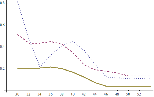
Given a LIF sampler with parameter and , Theorem 3.1 allows us to estimate the accuracy of signal reconstruction from LIF samples. Suppose a sequence of events given by , , then a signal reconstruction algorithm under consideration, such as that outlined in [4], reconstructs an approximate signal on the time interval . By re-sampling the signal we obtain a further sequence of events given by , . Since Theorem 3.1 guarantees quasi-isometry in terms of the inequalities (21) and (22), the computation of the discrepancy in the sample space, , according to (18) approximates the discrepancy measure in the signal space, , according to (17), where denotes the original input signal. See Fig. 2 for an example. This figure shows the reconstruction errors for different truncation parameters measured in three different ways: first, the discrepancy (18) measured in the sample space; second, the discrepancy (17) in the signal space, and, third, the max-norm between the original and the reconstructed signal. As expected, the error curves resulting from measuring the discrepancy in the signal and the sample space, respectively, have similar shapes. In particular, they have approximately the same basin of minimum. This means that parameter tuning can also be done in the sample space.
5 Conclusion
It is shown that leaky integrate-and-fire satisfies the condition of quasi-isometry if the metrics in the input as well as in the output space rely on Weyl’s discrepancy measure. The quasi-isometry relation is utilized for estimating the signal reconstruction error by means of re-sampling the reconstructed signal. An example is presented which demonstrates how numerical errors resulting from truncating summation in the reconstruction algorithm can be minimized this way. In future research we will exploit the outlined quasi-isometry approach as basis for developing a sound discrete mathematical framework for event-based signal and image processing.
Acknowledgment
The author would like to thank the Austrian COMET Program.
References
- [1] B. A. Moser and T. Natschläger, “On stability of distance measures for event sequences induced by level-crossing sampling.,” IEEE Transactions on Signal Processing, vol. 62, no. 8, pp. 1987–1999, 2014.
- [2] B. A. Moser, “Similarity recovery from threshold-based sampling under general conditions,” IEEE Trans. Signal Processing, vol. 65, no. 17, pp. 4645–4654, 2017.
- [3] B. A. Moser, “Geometric characterization of Weyl’s discrepancy norm in terms of its -dimensional unit balls,” Discrete and Computational Geometry, vol. 48, no. 4, pp. 793–806, 2012.
- [4] H. G. Feichtinger, J. C. Príncipe, J. L. Romero, A. Singh Alvarado, and G. A. Velasco, “Approximate reconstruction of bandlimited functions for the integrate and fire sampler,” Adv. Comput. Math., vol. 36, pp. 67–78, Jan. 2012.
- [5] M. M. Deza and E. Deza, Encyclopedia of Distances. Springer Berlin Heidelberg, 2009.
- [6] H. Weyl, “Über die Gleichverteilung von Zahlen mod. Eins,” Mathematische Annalen, vol. 77, pp. 313–352, 1916.
- [7] B. Chazelle, The Discrepancy Method: Randomness and Complexity. New York, NY, USA: Cambridge University Press, 2000.