Domain Reduction for Monotonicity Testing:
A $o(d)$ Tester for Boolean Functions in $d$-Dimensions

Monotonicity testing is a fundamental problem in property testing. Let $(D,\prec)$ be a partially ordered set (poset) and let $R$ be a total order. A function $f\colon D\to R$ is monotone if $f(x)\leq f(y)$ whenever $x\prec y$. The hypercube, $\{0,1\}^{d}$ and the hypergrid $[n]^{d}$ have been the most studied posets in monotonicity testing, where $\prec$ denotes the coordinate-wise partial ordering. The Hamming distance between two functions $f$ and $g$ is $\mathtt{dist}(f,g):=\mathbf{Pr}_{x\sim D}[f(x)\neq g(x)]$ where $x$ is drawn uniformly from the domain. The distance of $f$ to monotonicity, denoted $\varepsilon_{f}$, is its distance to the nearest monotone function. That is, $\varepsilon_{f}:=\min_{g\in{\mathcal{M}}}\mathtt{dist}(f,g)$, where ${\mathcal{M}}$ is the set of all monotone functions. A monotonicity tester is a randomized algorithm that makes queries to $f$ and accepts with probability $\geq 2/3$ if the function is monotone, and rejects with probability $\geq 2/3$ if $\varepsilon_{f}\geq\varepsilon$, where $\varepsilon\in(0,1)$ is an input parameter. The challenge is to determine the minimum query complexity of a monotonicity tester.

One of the earliest results in property testing is the $O(d/\varepsilon)$-query “edge-tester” due to Goldreich et al. [GGL+00] (see also [Ras99]) for testing monotonicity of Boolean functions over the hypercube, that is, $f\colon\{0,1\}^{d}\to\{0,1\}$. In the last few years, considerable work [CS14a, CST14, CDST15, KMS15, BB16, CWX17] has improved our understanding of Boolean monotonicity testing on the hypercube domain. In particular, Khot, Minzer, and Safra [KMS15] give an $\widetilde{O}(\sqrt{d}/\varepsilon^{2})$ query¹¹ 1 Throughout the paper $\widetilde{O}$ hides $\log(d/\varepsilon)$ factors., non-adaptive tester, and Chen, Waingarten, and Xie [CWX17] show that any tester (even adaptive) must make $\widetilde{\Omega}(d^{1/3})$ queries. In contrast, for real-valued functions over the hypercube $f\colon\{0,1\}^{d}\to\mathbb{R}$, the complexity is known to be $\Theta(d/\varepsilon)$ [DGL+99, BBM12, CS13, CS14b], that is, linear in $d$.

The problem of monotonicity testing Boolean functions $f\colon[n]^{d}\to\{0,1\}$ over hypergrids is not as well understood. Dodis et al. [DGL+99] (with improvements by Berman, Raskhodnikova, and Yaroslavtsev [BRY14a], henceforth BRY) give an $\widetilde{O}(d/\varepsilon)$-query tester. The important feature to note is the independence of $n$. Contrast this, again, with the real-valued case; monotonicity testing of functions $f\colon[n]\to\mathbb{R}$ requires $\Omega(\log n)$ queries [EKK+00, Fis04]. Recently, the authors [BCS18] describe an $\widetilde{O}(d^{5/6}\log^{4/3}n\penalty\ \varepsilon^{-4/3})$-query tester. Although the dependence on $d$ is sublinear, there is a dependence on $n$. The following question has remained open: Is there a monotonicity tester for functions $f\colon[n]^{d}\to\{0,1\}$, whose query complexity is independent of $n$ and sublinear in $d$? One of the main outcomes of this work is an affirmative answer to this question.

To gain perspective, the reader may restrict attention to functions defined over the continuous cube $[0,1]^{d}$, and assume the uniform measure $\mu$ on this cube. This is the natural generalization of property testing on the domains $\{0,1\}^{d}$ and $[n]^{d}$ as described above. The only restriction on the function we are testing is that the set of points where the function takes value $1$ (or $0$) must be (Lebesgue)-measurable. The distance between two functions $\mathtt{dist}(f,g):=\mathbf{Pr}_{x\sim\mu}[f(x)\neq g(x)]$ is the measure of the points at which they differ. The distance to monotonicity of a function $f$ is $\inf_{g\in{\mathcal{M}}}\mathtt{dist}(f,g)$ where ${\mathcal{M}}$ is the set of all monotone functions. (In general, we use any measure to define distance. For instance, we can test monotonicity of functions $f\colon\mathbb{R}^{d}\to\{0,1\}$ over the Gaussian measure.)

Note that the result of Theorem 1.2 holds for all measurable functions, with no dependence on surface area or “complexity” of $f$. This can be contrasted with the recent result of De, Mossel, and Neeman [DMN19], who showed that Junta testing of Boolean functions $f\colon\mathbb{R}^{d}\to\{0,1\}$ over the Gaussian measure requires some dependence on the surface area of $f$. Given the proof techniques for Theorem 1.1, the proof of Theorem 1.2 follows from standard measure theoretic methods. Nonetheless, we believe that there is a useful conceptual message in Theorem 1.2. It gives the natural “limit” of monotonicity testing for hypergrids $[n]^{d}$, as $n\rightarrow\infty$. This result also underscores the significance of getting testers independent of $n$ (for hypergrids), since it leads to testers for all measurable functions.

The theorem is a direct corollary of the following lemma, applied to each dimension.

This lemma is the heart of our results, and in this section we give an overview of its proof. Let us start with the simple case of $d=1$ (the line). Monotonicity testers for the line immediately imply domain reduction for $d=1$ [DGL+99, BRY14a]. A u.a.r. sample of $\widetilde{O}(1/\varepsilon_{f})$ points in $[n]$ contains a monotonicity violation with large probability ($>9/10$, say), and thus the restriction of $f$ to this sample has distance $\widetilde{\Omega}(\varepsilon_{f})$. However, $\Omega(\varepsilon_{f})$ is weak for what we need since, even if one could generalize this argument to the setting of Lemma 2.1, we would need to apply it $d$ times to get the full domain reduction (Theorem 1.3). This would imply a final lower bound of $\varepsilon_{f}/C^{d}$, for some constant $C$, which has little value towards proving a sublinear-in-$d$ query tester.

Fortunately, quantitatively stronger domain reduction exists for the line. BRY ([BRY14a], Theorem 3.1) proves that if one samples $\Theta(s^{2}/\varepsilon_{f})$ points, then the expected distance of the restricted function is at least $\varepsilon_{f}(1-1/s)$. Numerically speaking, this is encouraging news, since we could try to set $s=\Theta(d)$ and iterate this argument $d$ times (over each dimension). Of course, this result for the line alone is not enough to deal with the structure of general hypergrids, but forms a good sanity check.

Consider the general case of Lemma 2.1. For brevity, we let $D:=[n]\times\left(\prod_{i=2}^{d}[n_{i}]\right)$ and $D_{T}:=T\times\left(\prod_{i=2}^{d}[n_{i}]\right)$ denote the original and reduced domains, respectively. Note that $|D_{T}|=\frac{k}{n}|D|$.

The standard handle on the distance to monotonicity is the violation graph of $f$, arguably first formalized by Fischer et al. [FLN+02]. The graph has vertex set $D$ and an edge $(x,y)$ iff $x\prec y$ and $f(x)=1,f(y)=0$. A theorem of [FLN+02] states that any maximum cardinality matching $M$ in the violation graph satisfies $|M|=\varepsilon_{f}|D|$. Fix such a matching $M$. For a fixed sample $T$, we let $M_{T}$ denote a maximum cardinality matching in the violation graph of $f_{T}$. To argue about $\varepsilon_{f_{T}}$, we want to give a lower bound on the expected size $|M_{T}|$. To do so, we give a lower bound the expected number of endpoints of $M$ that can still be matched (simultaneously) in the violation graph of $f_{T}$.

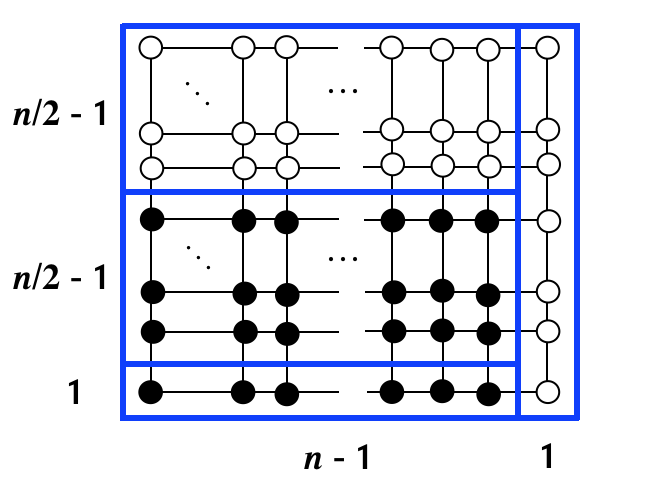
We use the following standard notions of lines and slices in $D$, with respect to the first dimension. Refer to Fig. 1 and Fig. 2 for visual examples in two dimensions. In these examples the rows represent the lines while the columns represent the slices. Below, for $x\in D$, the vector $x_{-1}$ is used to denote $(x_{2},x_{3},\ldots,x_{d})$.

• •

  (Lines in $D$) ${\mathcal{L}}:=\left\{\ell_{z}:z\in\prod_{i=2}^{d}[n_{i}]\right\}$ where $\ell_{z}:=\left\{x\in D:x_{-1}=z\right\}$.

• •

  (Slices in $D$) $\mathcal{S}:=\left\{S_{i}:i\in[n]\right\}$ where $S_{i}:=\left\{x\in D:x_{1}=i\right\}$.

We partition $M$ into a collection of “local” matchings for each line:

• •

  (Line Decomposition of $M$) For each $\ell\in{\mathcal{L}}$: $M^{(\ell)}:=\{(x,y)\in M:x\in\ell\}$.

We find a large matching in the violation graph of $f_{T}$ by doing a line-by-line analysis. In particular, for each line $\ell\in{\mathcal{L}}$, we define the following matching $M^{(\ell)}_{T}$ in the violation graph of $f_{T}$.

• •

  (The matching $M^{(\ell)}_{T}$) For each $\ell\in{\mathcal{L}}$, consider the collection of all maximum cardinality violation matchings w.r.t. $f_{T}$ on the set of vertices that (a) are matched by $M^{(\ell)}$, and (b) lie in some slice $S_{i}$ where $i\in T$. We let $M^{(\ell)}_{T}$ denote any such fixed matching.

We stress that $M^{(\ell)}_{T}$ is not a subset of $M^{(\ell)}$, but the endpoints of the pairs in $M^{(\ell)}_{T}$ are a subset of the endpoints of the pairs in $M^{(\ell)}$. Thus, by the above definition, the union $M_{T}:=\cup_{\ell\in{\mathcal{L}}}M_{T}^{(\ell)}$ is a valid matching in the violation graph of $f_{T}$ since $M^{(\ell)}$ and $M^{(\ell^{\prime})}$ have disjoint endpoints for all $\ell\neq\ell^{\prime}\in{\mathcal{L}}$. We will lower bound the size of this matching, $|M_{T}|$, by giving a lower bound on $|M_{T}^{(\ell)}|$ for each line $\ell$.

Fix some $\ell\in{\mathcal{L}}$. By definition, the lower-endpoints of $M^{(\ell)}$ all lie on $\ell$, and thus are all comparable. Let $M^{(\ell)}=\{(x_{1},y_{1}),\ldots,(x_{m},y_{m})\}$ where $x_{1}\prec\cdots\prec x_{m}$ and observe that, for any $j\in[m]$, $x_{1},\ldots,x_{j}\prec y_{j},\ldots,y_{m}$. Since the function is Boolean, every $x\in\{x_{1},\ldots,x_{j}\}$ forms a violation to monotonicity with every $y\in\{y_{j},\ldots,y_{m}\}$, and therefore these vertices can be matched in $M^{(\ell)}_{T}$, if their $1$-coordinates are sampled by $T$.

Since all the $x_{i}$’s lie on the same line $\ell$, their $1$-coordinates are distinct. Suppose that the $1$-coordinates of all the $y_{i}$’s were also distinct and distinct from those of the $x_{i}$’s too. Under this assumption we can proceed with our analysis as if all the $x_{i}$’s and $y_{i}$’s lie on $\ell$, and the analysis becomes identical to the one-dimensional case. We could thus apply Theorem 3.1 of [BRY14a] to each $\ell\in{\mathcal{L}}$ to prove Lemma 2.1. However, the assumption that the $y_{i}$’s have distinct $1$-coordinates is far from the truth. As we explain below, there are examples where all the $y_{i}$’s have the same $1$-coordinate, thereby lying in the same slice $S_{a}$ (for some $a\in[n]$). In this case, with probability $(1-k/n)$ we would have the size of $M^{(\ell)}_{T}$ be $0$ (if $a\notin T$), implying that $\mathbf{E}_{T}\left[|M^{(\ell)}_{T}|\right]$ could be as small as $(k/n)^{2}\cdot|M^{(\ell)}|$. Thus, if there existed a function $f$ such that a “collision of $y$’s $1$-coordinates” could not be avoided for a large number of lines, then this would preclude such a line-by-line approach to proving Lemma 2.1. Unfortunately, there are examples of violation matchings where this happens. Consider Example 1, and the left part of Fig. 2, shown at the end of this section. For the lowest line, all the corresponding $y$’s in $M^{(\ell)}$ have the same $1$-coordinate.

Our main insight is that for any $f$, there always exists a violation matching $M$ where the problem above does not arise too often. This motivates the key definition of stacks; the stacks are what determine the “shape” of a matching. Formally, for any $\ell\in{\mathcal{L}}$ and $S\in\mathcal{S}$, the $(\ell,S)$-stack is the set of pairs $(x,y)\in M$, where $x\in\ell$ and $y\in S$.

• •

  (Stacks) $M^{(\ell,S)}:=\{(x,y)\in M^{(\ell)}:y\in S\}=\{(x,y)\in M:x\in\ell,y\in S\}$.

We call $|M^{(\ell,S)}|$ the “size of the stack $(\ell,S)$”. To summarize the above discussion, small stacks are good news while big stacks are bad news. This is formalized in Lemma 2.3.

If there is a maximum cardinality matching $M$ in the violation graph of $f$ such that all stacks have size at most $1$, then the one-dimensional domain reduction can be directly applied. Unfortunately, this is not possible. We give an example in Fig. 1 of a function where stacks of size at least $2$ are unavoidable³³ 3 Interestingly, we don’t know of a function where stacks of size strictly larger than $2$ can’t be avoided. In fact, we can prove that for the grid (the $d=2$ case) one can always find a maximum cardinality violation matching $M$ where $|M^{(\ell,S)}|\leq 3$ for all $(\ell,S)$. The proof is cumbersome and so we exclude it since it is not relevant to our main result.. One reason for this difficulty may be that there can be various maximum cardinality matchings in the violation graph that have vastly different stack sizes (shapes); again consider Example 1. Nevertheless, we prove that there is a matching $M$ such that for every positive integer $\lambda$, the total number of pairs belonging to stacks of size at least $\lambda$ is at most $|D|/\mathrm{poly}(\lambda)$.

The main creativity to prove this lemma lies in the choice of $M$. Given a matching, we define the vector $\Lambda(M)$ that enumerates all the stack sizes in non-decreasing order. We show that the maximum cardinality matching $M$ with the lexicographically largest $\Lambda(M)$ serves our purpose. That is, we choose $M$ that maximizes the minimum stack size, and then subject to this maximizes the second minimum, and so on. It may seem counter-intuitive that we want a matching with small stack sizes, and yet our potential function maximize the minimum. The intuitive explanation is that the sum of the stack sizes is $|M|$, which is fixed, and so in a sense maximizing the minimum also balances out the $\Lambda(M)$ vector. The proof uses a matching rewiring argument to show that any large stack must be “adjacent” to many moderate size stacks. If two stacks are appropriately “aligned”, one could change the matching to move points from one stack to the other. Large stacks cannot be aligned with small stacks, since one could rewire the matching to increase the potential. But since the function is Boolean one can show that there are many opportunities for rewiring the violation matching. Thus, there isn’t enough “room” for many large stacks. We then apply some technical charging arguments to bound the total number of points in large stacks. The full proof is given in §4.

With the stack bound in hand, we need to generalize the one-dimensional argument of BRY (Theorem 3.1 [BRY14a]) to account for bounded stack sizes. Then, we bound $|M^{(\ell)}_{T}|$ for all $\ell$, and get the final lower bound on the distance $\varepsilon_{f_{T}}$.

The proof is a fairly straightforward generalization of the arguments in [BRY14a] for the $\lambda=1$ case. The idea is to control the size of the maximum cardinality matching $M^{(\ell)}_{T}$ by analyzing the discrepancy of a random subsequence of a sequence of $1$s and $0$s. For the sake of simplicity, we give a proof that achieves a weaker dependence on $\varepsilon_{f}$ than in [BRY14a]. Our proof of Lemma 2.3 is given in §5. We note that BRY give a stronger lower bound (without the $\sqrt{\ln k}$) and also bound the variance for the $\lambda=1$ case. A more careful generalization of BRY which removes the $\sqrt{\ln k}$ would yield an improved loss of $C/k^{1/6}$ instead of $C/k^{1/7}$ in Lemma 2.1, but we prefer to give the simpler $C/k^{1/7}$ exposition for the purpose of ease of reading.

In this section, we use Lemma 2.2 and Lemma 2.3 to prove Lemma 2.1. Recall that $D:=[n]\times\left(\prod_{i=2}^{d}[n_{i}]\right)$ and $D_{T}:=T\times\left(\prod_{i=2}^{d}[n_{i}]\right)$ denote the original and reduced domains, respectively. Note that $|D_{T}|=\frac{k}{n}|D|$. Let $M$ be the matching given by Lemma 2.2 and consider $\lambda=\left\lceil 25k^{2/7}\right\rceil$. Clearly, $\lambda\in[25k^{2/7},26k^{2/7}]$.

In this proof, our goal is to construct a matching $M_{T}$ in the violation graph of $f_{T}$ whose cardinality is sufficiently large. We measure $\mathbf{E}_{T}\left[|M_{T}|\right]$ by summing over all lines in ${\mathcal{L}}$ and applying Lemma 2.3 to each. Notice that $\widehat{M}$ is a matching in the violation graph of $f$ which satisfies $|\widehat{M}^{(\ell,S)}|\leq 26k^{2/7}$ for all $\ell\in{\mathcal{L}}$ and $S\in\mathcal{S}$. Thus by Lemma 2.3, for every $\ell\in{\mathcal{L}}$,

We are given a Boolean function $f\colon D\to\{0,1\}$ where $D=[n]\times\left(\prod_{i=2}^{d}[n_{i}]\right)$ is a rectangular hypergrid for some $n,n_{2},\ldots,n_{d}\in\mathbb{Z}^{+}$. Lemma 2.2 asserts there is a maximum cardinality matching $M$ such that $\sum_{(\ell,S):|M^{(\ell,S)}|\geq\lambda}|M^{(\ell,S)}|\leq\frac{5}{\sqrt{\lambda}}\cdot|D|$ for all $\lambda\in\mathbb{Z}^{+}$.

Given a matching $M$, we consider the vector (or technically, the list) $\Lambda(M)$ indexed by stacks $(\ell,S)$ with $\Lambda_{\ell,S}:=|M^{(\ell,S)}|$, and list these in non-decreasing order. Consider the maximum cardinality matching $M$ in the violation graph of $f$ which has the lexicographically largest $\Lambda(M)$. That is, the minimum entry of $\Lambda(M)$ is maximized, and subject to that the second-minimum is maximized and so on. We fix this matching $M$ and claim that it satisfies $\sum_{(\ell,S):|M^{(\ell,S)}|\geq\lambda}|M^{(\ell,S)}|\leq\frac{5}{\sqrt{\lambda}}\cdot|D|$ for all $\lambda\in\mathbb{Z}^{+}$. Note that the inequality is trivial for $\lambda\leq 100$, since $M$ itself is of size at most $\varepsilon_{f}|D|\leq\frac{1}{2}|D|$. Thus, in what follows we prove that the inequality is true for an arbitrary, fixed $\lambda>100$. We first introduce the following notation.

• •

  (Low Stacks) $L:=\{(\ell,S)\in{\mathcal{L}}\times\mathcal{S}:|M^{(\ell,S)}|\leq\lambda-2\}$.

• •

  (High Stacks) $H:=\{(\ell,S)\in{\mathcal{L}}\times\mathcal{S}:|M^{(\ell,S)}|\geq\lambda\}$.

Let $V(H)$ denote the set of vertices matched by $\bigcup_{(\ell,S)\in H}M^{(\ell,S)}$. Let $B$ (for blue) be the set of points in $V(H)$ with function value $0$, and $R$ (for red) be the set of points in $V(H)$ with function value $1$. $M$ induces a perfect matching between $B$ and $R$, and we wish to prove $|B|=|R|\leq\frac{5}{\sqrt{\lambda}}\cdot|D|$. Indeed, define $\delta$ to be such that $|B|=\delta|D|$. In the remainder of the proof, we will show that $\delta\leq\frac{5}{\sqrt{\lambda}}$.

We make a simple observation that for any fixed line $\ell$, there cannot be too many non-low stacks $(\ell,S)$.

We show that if the number of blue points $|B|$ is large ($>5|D|/\sqrt{\lambda}$), then we will find a line participating in more than $n/(\lambda-1)$ non-low stacks. To do so, we need to “find” these non-low stacks. We need some more notation to proceed. For a vertex $z$, we let $\ell_{z}$ ($S_{z}$, resp.) denote the unique line (slice, resp.) containing $z$. For each blue point $y\in B$, we define the following interval

Note that ${\mathcal{I}}_{y}$ is the interval of $\ell_{y}$ whose endpoints are given by the projection of $(x,y)$ onto $\ell_{y}$. Armed with this notation, we can find our non-low stacks. Our next claim, which is the heart of the proof and uses the potential function, shows that for every high stack $(\ell,S)$, we get a bunch of other “non-low” stacks participating with the line $\ell$. Refer to Fig. 3 for an accompanying illustration of the proof.

The rest of the proof is a (slightly technical) averaging argument to prove that $|B|$ is small. We introduce some more notation to carry this through. For a blue point $y\in B$, let $\beta_{y}:=\frac{|{\mathcal{I}}_{y}\cap B|}{|{\mathcal{I}}_{y}|}$ denote the fraction of blue points in ${\mathcal{I}}_{y}$. For $\alpha\in(0,1)$, we say that $y\in B$ is $\alpha$-rich if $\beta_{y}\geq\alpha$. A point $x\in R$ is $\alpha$-rich if its blue partner $y\in B$ (i.e. $(x,y)\in M$) is $\alpha$-rich. We also call the pair $(x,y)$ an $\alpha$-rich pair. For what follows, recall that $\delta\in(0,1)$ is defined such that $|B|=\delta|D|$.

References

- [AC06] Nir Ailon and Bernard Chazelle. Information theory in property testing and monotonicity testing in higher dimension. Information and Computation, 204(11):1704–1717, 2006.
- [ACCL07] Nir Ailon, Bernard Chazelle, Seshadhri Comandur, and Ding Liu. Estimating the distance to a monotone function. Random Structures Algorithms, 31(3):371–383, 2007.
- [BB16] Aleksandrs Belovs and Eric Blais. A polynomial lower bound for testing monotonicity. In Proceedings, ACM Symposium on Theory of Computing (STOC), 2016.
- [BBM12] Eric Blais, Joshua Brody, and Kevin Matulef. Property testing lower bounds via communication complexity. Computational Complexity, 21(2):311–358, 2012.
- [BCS18] Hadley Black, Deeparnab Chakrabarty, and C. Seshadhri. A monotonicity tester for Boolean functions over the hypergrid . In Proceedings, ACM-SIAM Symposium on Discrete Algorithms (SODA), 2018.
- [BCSM12] Jop Briët, Sourav Chakraborty, David García Soriano, and Ari Matsliah. Monotonicity testing and shortest-path routing on the cube. Combinatorica, 32(1):35–53, 2012.
- [BGJ+12] Arnab Bhattacharyya, Elena Grigorescu, Madhav Jha, Kyoming Jung, Sofya Raskhodnikova, and David Woodruff. Lower bounds for local monotonicity reconstruction from transitive-closure spanners. SIAM Journal on Discrete Mathematics (SIDMA), 26(2):618–646, 2012.
- [Bha08] Arnab Bhattacharyya. A note on the distance to monotonicity of boolean functions. Technical Report 012, Electronic Colloquium on Computational Complexity (ECCC), 2008.
- [BRY14a] Piotr Berman, Sofya Raskhodnikova, and Grigory Yaroslavtsev. -testing. In Proceedings, ACM Symposium on Theory of Computing (STOC), 2014.
- [BRY14b] Eric Blais, Sofya Raskhodnikova, and Grigory Yaroslavtsev. Lower bounds for testing properties of functions over hypergrid domains. In Proceedings, IEEE Conference on Computational Complexity (CCC), 2014.
- [CDJS15] Deeparnab Chakrabarty, Kashyap Dixit, Madhav Jha, and C. Seshadhri. Property testing on product distributions: Optimal testers for bounded derivative properties. In Proceedings, ACM-SIAM Symposium on Discrete Algorithms (SODA), 2015.
- [CDST15] Xi Chen, Anindya De, Rocco A. Servedio, and Li-Yang Tan. Boolean function monotonicity testing requires (almost) non-adaptive queries. In Proceedings, ACM Symposium on Theory of Computing (STOC), 2015.
- [CS13] Deeparnab Chakrabarty and C. Seshadhri. Optimal bounds for monotonicity and Lipschitz testing over hypercubes and hypergrids. In Proceedings, ACM Symposium on Theory of Computing (STOC), 2013.
- [CS14a] Deeparnab Chakrabarty and C. Seshadhri. An monotonicity tester for Boolean functions over the hypercube. SIAM Journal on Computing (SICOMP), 45(2):461–472, 2014.
- [CS14b] Deeparnab Chakrabarty and C. Seshadhri. An optimal lower bound for monotonicity testing over hypergrids. Theory of Computing, 10:453–464, 2014.
- [CST14] Xi Chen, Rocco A. Servedio, and Li-Yang. Tan. New algorithms and lower bounds for monotonicity testing. In Proceedings, IEEE Symposium on Foundations of Computer Science (FOCS), 2014.
- [CWX17] Xi Chen, Erik Waingarten, and Jinyu Xie. Beyond talagrand: New lower bounds for testing monotonicity and unateness. In Proceedings, ACM Symposium on Theory of Computing (STOC), 2017.
- [DGL+99] Yevgeny Dodis, Oded Goldreich, Eric Lehman, Sofya Raskhodnikova, Dana Ron, and Alex Samorodnitsky. Improved testing algorithms for monotonicity. Proceedings, International Workshop on Randomization and Computation (RANDOM), 1999.
- [DMN19] Anindya De, Elchanan Mossel, and Joe Neeman. Is your function low dimensional? In Conference on Learning Theory, COLT 2019, 25-28 June 2019, Phoenix, AZ, USA, pages 979–993, 2019.
- [EKK+00] Funda Ergun, Sampath Kannan, Ravi Kumar, Ronitt Rubinfeld, and Mahesh Viswanathan. Spot-checkers. J. Comput. System Sci., 60(3):717–751, 2000.
- [Fis04] Eldar Fischer. On the strength of comparisons in property testing. Information and Computation, 189(1):107–116, 2004.
- [FLN+02] Eldar Fischer, Eric Lehman, Ilan Newman, Sofya Raskhodnikova, and Ronitt Rubinfeld. Monotonicity testing over general poset domains. Proceedings, ACM Symposium on Theory of Computing (STOC), 2002.
- [FR10] Shahar Fattal and Dana Ron. Approximating the distance to monotonicity in high dimensions. ACM Trans. on Algorithms (TALG), 6(3), 2010.
- [GGL+00] Oded Goldreich, Shafi Goldwasser, Eric Lehman, Dana Ron, and Alex Samordinsky. Testing monotonicity. Combinatorica, 20:301–337, 2000.
- [Gol17] Oded Goldreich. Introduction to property testing. Cambridge University Press, 2017.
- [HK03] Shirley Halevy and Eyal Kushilevitz. Distribution-free property testing. Proceedings, International Workshop on Randomization and Computation (RANDOM), 2003.
- [HK08] Shirley Halevy and Eyal Kushilevitz. Testing monotonicity over graph products. Random Structures Algorithms, 33(1):44–67, 2008.
- [KMS15] Subhash Khot, Dor Minzer, and Muli Safra. On monotonicity testing and Boolean isoperimetric type theorems. In Proceedings, IEEE Symposium on Foundations of Computer Science (FOCS), 2015.
- [LR01] Eric Lehman and Dana Ron. On disjoint chains of subsets. Journal of Combinatorial Theory, Series A, 94(2):399–404, 2001.
- [Nel15] Gail S. Nelson. A user-friendly introduction to Lebesgue measure and integration, volume 78. American Mathematical Soc., 2015.
- [PRR06] Michal Parnas, Dana Ron, and Ronitt Rubinfeld. Tolerant property testing and distance approximation. Journal of Computer and System Sciences, 6(72):1012–1042, 2006.
- [Ras99] Sofya Raskhodnikova. Monotonicity testing. Masters Thesis, MIT, 1999.
- [RRSW11] Dana Ron, Ronitt Rubinfeld, Muli Safra, and Omri Weinstein. Approximating the Influence of Monotone Boolean Functions in Query Complexity. In Proceedings, International Workshop on Randomization and Computation (RANDOM), 2011.
- [SS05] Elias Stein and Rami Shakarchi. Real Analysis: Measure Theory, Integration, and Hilbert Spaces. Princeton University Press, 2005.
- [SS08] Michael E. Saks and C. Seshadhri. Parallel monotonicity reconstruction. In Proceedings, ACM-SIAM Symposium on Discrete Algorithms (SODA), 2008.