Predictive Deployment of UAV Base Stations in Wireless Networks: Machine Learning Meets Contract Theory A preliminary version of this work appears in the proceedings of IEEE GLOBECOM 2018 [1]. This research was supported by the U.S. National Science Foundation under Grant IIS-1633363.
Abstract
In this paper, a novel framework is proposed to enable a predictive deployment of unmanned aerial vehicles (UAVs) as temporary base stations (BSs) to complement ground cellular systems in face of downlink traffic overload. First, a novel learning approach, based on the weighted expectation maximization (WEM) algorithm, is proposed to estimate the user distribution and the downlink traffic demand. Next, to guarantee a truthful information exchange between the BS and UAVs, using the framework of contract theory, an offload contract is developed, and the sufficient and necessary conditions for having a feasible contract are analytically derived. Subsequently, an optimization problem is formulated to deploy an optimal UAV onto the hotspot area in a way that the utility of the overloaded BS is maximized. Simulation results show that the proposed WEM approach yields a prediction error of around . Compared with the expectation maximization and k-mean approaches, the WEM method shows a significant advantage on the prediction accuracy, as the traffic load in the cellular system becomes spatially uneven. Furthermore, compared with two event-driven deployment schemes based on the closest-distance and maximal-energy metrics, the proposed predictive approach enables UAV operators to provide efficient communication service for hotspot users in terms of the downlink capacity, energy consumption and service delay. Simulation results also show that the proposed method significantly improves the revenues of both the BS and UAV networks, compared with two baseline schemes.
Index Terms – cellular networks; UAV deployment; traffic prediction; contract theory.
I introduction
The use of unmanned aerial vehicles (UAVs) as flying base stations (BSs) has attracted growing interest in the past few years [2, 1, 3, 4, 5, 6, 7, 8]. UAVs can be deployed to complement the existing cellular systems, by providing reliable wireless services for ground users, to potentially increase the network capacity, eliminate coverage holes, and cope with the steep surge of communication needs during hotspot events [1]. Compared with the terrestrial BSs that are deployed at a fixed location for a long term, UAVs are more suitable for temporary on-demand service [3]. For instance, UAVs can provide communication service for major events (e.g. sport or musical events) during which the terrestrial network capacity is often strained [4]. Furthermore, UAVs can adjust their positions and establish line-of-sight (LOS) communication links towards ground users, thus improving network performance [5]. Due to their broad range of application domains and low cost, UAVs is a promising solution to provide temporary connectivity for ground users[6].
However, the UAV deployment for on-demand cellular service faces several key challenges. For instance, UAVs are strictly constrained by their on-board energy, which should be efficiently used for communication. However, the on-demand deployment requires UAVs to continuously change their positions to meet instant communication requests. Therefore, most of on-board energy can be consumed by mobility, thus limiting their communication capabilities [1]. Moreover, to effectively alleviate network congestion during a hotspot event, the deployed UAV must have enough on-board power to satisfy the downlink communication demand. To allocate a qualified UAV with sufficient energy, the network operator should estimate the required transmit power, based on the real-time traffic load. These challenges, in turn, motivate the need for a comprehensive prediction of cellular traffic, and a predictive approach for UAV deployment [9]. To this end, machine learning (ML) techniques can be applied to estimate the cellular traffic demand within the target system. Given the predicted traffic load, each BS can detect hotspot areas and request suitable UAVs to alleviate network congestion.
Another challenge of the on-demand deployment for aerial wireless service is to incentivize cooperation between the ground BS and the UAV operators under the asymmetric information. As shown in [10], the ground BSs and UAVs can belong to different operators who seek to selfishly maximize their individual benefits. Hence, to request a UAV’s assistance, a ground BS must offer an appropriate economic reward to the UAV operator for aerial wireless service. However, given that the BS has no prior knowledge of each UAV, there is no guarantee that the requested UAV is able to provide enough transmit power to satisfy the downlink demand. Therefore, designing an incentive mechanism is necessary to ensure a truthful information exchange between the UAV and BS systems, when the information among different network operators is asymmetric.
I-A Related Works
The optimal deployment of UAVs for cellular service has been studied in [11, 12, 13]. In [11], the authors studied the optimal locations and coverage areas of UAVs that minimizes the transmit power. The work in [12] derived the minimum number of UAVs needed to satisfy the coverage and capacity constraints. In [13], the authors jointly optimized the UAV trajectory and the network resource allocation to maximize the throughput to ground users. The problem of traffic offloading from an existing wireless network to UAVs has been addressed in [14, 15, 16, 17]. In [14], the allocation problem of UAVs to each geographic area was investigated to improve the spectral efficiency and reduce the delay. In [15] and [16], the authors optimized the trajectory of UAVs to provide wireless services to the cell-edge users. In [17], an unsupervised learning approach was presented to solve the deployment of a fleet of UAVs for traffic offloading. However, most of the existing works [11, 12, 13, 14, 15, 16, 17] assumed that the traffic demand of the cellular users is known a priori, which is challenging to estimate in a practical network. Furthermore, the works [11, 12, 13, 14, 15, 16, 17] optimized the performance of the cellular network in a centralized approach which assumes all UAVs belong to the same entity. Given the fact that the UAVs can belong to multiple operators, a new framework is needed to consider the individual utility of UAVs in the aerial communication service, while optimizing the performance of the ground cellular networks.
Meanwhile, in [18, 19, 20], a number of ML approaches are proposed to predict the traffic demands of cellular networks. In [18], a prediction framework is proposed to model the cellular data in the temporal and spatial domains. The authors in [19] predicted the locations of users during daily activities, based on pattern modeling. The work [20] provided surveys that focused on the general use of ML algorithms in cellular networks. Furthermore, the prior art in [21, 22, 23] studied the use of ML techniques to improve the performance of UAV-aided communications. In [21], an ML framework based on liquid state machine is proposed to optimize the caching content and resource allocation for each UAV. In [22], the authors investigated an ML approach to construct a radio map for autonomous path planning of UAVs. In [23], ML algorithms are applied to detect aerial users from the ground mobile users. However, most of the works in [18, 19, 20, 21, 22, 23] aim to build an ML model to predict regular traffic patterns, while hotspot events are considered as an anomaly and excluded from these studies. In fact, none of the approaches proposed in [18, 19, 20, 21, 22, 23] can effectively identify the hotspot areas or accurately predict excessive traffic load during the hotspot event. Thus, results of these prior works cannot enable a predictive UAV deployment for on-demand cellular service to alleviate the traffic congestion.
I-B Contributions
The main contribution of this paper is a novel framework for optimally deploying UAVs to assist a ground cellular network in alleviating its downlink traffic congestion during hotspot events. The proposed framework divides the deployment process into four, inter-related and sequential stages: learning stage, association stage, movement stage, and service stage. For each stage, we evaluate the performance of the proposed framework, using an open-source dataset in [24]. Our main contributions include:
- •
A novel framework, based on the weighted expectation maximization (WEM) approach, is proposed to predict the downlink traffic demand for each cellular system in the learning stage. The proposed WEM method is a general version of the conventional expectation maximization (EM) algorithm, which enables a variable weight at each data point in the distribution modeling. In particular, the proposed approach identifies the user distribution, predicts the cellular data demand, and pinpoints the hotspot areas within the cellular system.
- •
In the association stage, to employ a UAV with sufficient on-board energy to satisfy the downlink demand, the framework of contract theory [25] is introduced, where each overloaded BS can jointly design the transmit power and unit reward of the target UAV. We analytically derive the sufficient and necessary conditions needed to guarantee a truthful information exchange between the BS and UAV operators. The proposed contract approach yields little communication overhead and exhibits a low computational complexity.
- •
Simulation results show that the mean relative error (MRE) of the proposed ML approach is around . Compared with two baselines, an EM scheme and a -mean algorithm, the proposed method yields a better prediction accuracy, particularly when the downlink traffic load in the cellular system becomes spatially uneven. Furthermore, simulation results show that the designed contract ensures a non-negative payoff of each UAV, and each UAV will truthfully reveal its communication capability by accepting the contract designed for itself.
- •
We evaluate the performance of the proposed approach with two event-driven allocation methods, based on the closest-distance and maximal-energy metrics, that deploy a target UAV after the network congestion occurs, without traffic prediction and contract design. Numerical results show that the proposed predictive method enables UAV operators to provide efficient downlink service for hotspot users, in terms of the downlink capacity, energy consumption, and service delay. Moreover, the proposed method significantly improves the economic revenues of both the BS and UAV networks, compared with two baseline schemes.
The rest of this paper is organized as follows. In Section II, we present the system model. The problem formulation is given in Section III. In Section IV, the ML approach is proposed to predict downlink traffic demands. In Section V, the feasible contract is designed with the optimal UAV being employed to offload the cellular traffic. Simulation results are presented in Section VI. Finally, conclusions are drawn in Section VII.
II System Model
Consider a set of cellular BSs providing downlink wireless service to a group of user equipments (UEs) in a geographical area . Each BS serves an area , such that , and for any . The spatial distribution of the served UEs for each BS is denoted by , where . A set of flying UAVs can provide additional cellular service, if the hotspot events happen in the ground cellular network. We assume that the group BSs and UAVs belong to different network operators, and different frequency bands are used for the ground and aerial downlink transmissions, separately. A single antenna is equipped at each UE that can receive signals from both the ground BS and the UAV. Initially, a UE will connect to one of the ground BSs. However, as shown in Fig. 1, if a ground BS is overloaded in the downlink, BS can request the assistant of a UAV to offload the service of some UEs. We assume that a UAV only serves the UEs of a single BS at each time, while each BS can employ multiple UAVs, based on the cellular traffic demand. In this regard, if the downlink traffic demand at the level of a given BS is excessive, such that no single UAV is capable to alleviate traffic congestion, then the BS will divide the offloaded UEs into multiple spatially-disjoint sets, and request an individual UAV for each UE set, independently. Meanwhile, each UAV is equipped with a directional antenna array that enables beamforming transmissions [26]. As a result, interference between different UAV networks is negligible.

II-A Air-to-ground downlink communications
The path loss of the air-to-ground communication link from a typical UAV located at to a typical ground UE that is located at can be given by [27]:
| (1) |
where is the carrier frequency of UAV downlink communications, is the UAV-UE distance, is the speed of light, and is the additional path loss of the air-to-ground channel, compared with the free space propagation. The value of can be modeled as a Gaussian distribution with different parameters and for the LOS and non-line-of-sight (NLOS) links, respectively. Then, the achievable data rate from a UAV located at to a UE located at is
| (2) |
where is the downlink bandwidth of each UAV, is the antenna gain of UAV towards the UE located at , is the transmit power of UAV , is the path loss in linear scale, and is the average noise power spectrum density at the UE. The probability of having a LOS link between UAV located at and the UE located at is given by [28]:
| (3) |
where and are constant values that depend on the communication environment, is the elevation angle, and is the altitude of UAV . Consequently, the average downlink rate between a UAV and a UE at will be:
| (4) |
In order to serve multiple downlink UEs, each UAV applies a time-division-multiple-access (TDMA) technique11 1 The focus of this work is on the deployment stage and, hence, we do not optimize the multiple access scheme type or operation. Optimizing multiple access can be done post-deployment and will be subject to future work. that divides the time resource evenly among all served UEs, and all bandwidth will be allocated to one single UE during each time slot [29]. By using suitable uplink control signals, the UAV-UE channel can be accurately measured, and thus, the beamforming of UAV’s antennas can be properly optimized towards the served UE. Consequently, the average rate that UAV can provide to the hotspot UEs from BS will be
| (5) |
where is the hotspot area, is the normalized spatial distribution of UEs within , and . When downlink congestion occurs, BS detects the congested area and offloads the UEs within to the target UAV.
| Notation | Description | Notation | Description |
|---|---|---|---|
| , | Number of BSs and number of UAVs | Movement time of UAV to the service location of BS | |
| Interval of the UAV’s offloading service | Average rate of UAV to each hotspot user of BS | ||
| Location of a ground user | Average rate of UAV to all hotspot users of BS | ||
| , | Current location of UAV , and service location of UAV associated with BS | Amount of data that UAV provides to all hotspot users of BS within one | |
| User distribution and data demand distribution of BS | , | Average rate demand per user/ hotspot user of BS | |
| , | Service area and hotspot area of BS | Utility of BS by employing UAV | |
| , | Number of all users and number of hotspot users of BS | Utility of UAV by providing offloading service to BS | |
| Data demand of hotspot users within one of BS | Type of UAV with respect to BS | ||
| Transmit power of UAV | , | Weight vectors in the user and demand distribution models | |
| Unit payment of BS | , | Mean and covariance of Gaussian distribution |
II-B UAV deployment process

Given the average downlink rate of each UAV in (5), the next step is to deploy suitable UAVs to offload the traffic and alleviate the downlink congestion in the ground cellular network. To facilitate the analysis, we assume that the service interval of each UAV a constant . As shown in Fig. 2, the deployment process has four sequential stages: learning stage, association stage, movement stage, and service stage. The details of each stage are given as next:
II-B1 Learning stage
For each BS , once the downlink traffic exceeds its network capacity, a learning stage with a fixed duration starts. During , BS collects the transmission record , where is the data rate that BS provides to the UE located at at time , and is the time slot during which the downlink rate can be considered to be constant. Given that the hotspot area and the UE distribution is unknown, a learning stage is necessary for BS to estimate the spatial distribution of UEs and the traffic demand of the on-going hotspot event. Considering common events, such as sport games and outdoor concerts, where mobile users are often confined to seat or geographically constrained spaces, the mobility of hotspot UEs is scarce. Thus, we assume that the UE distribution during one is time-invariant. Furthermore, to estimate the traffic demand within the congested area, a spatial density function is proposed to evaluate the average data rate per UE at each location . The proposed approach for estimating the UE distribution and traffic demand will be discussed in Section IV. Consequently, the total data demand from a hotspot area during a time interval will be given by:
| (6) |
Next, the BS will estimate the necessary number of UAVs to alleviate downlink congestion and calculate the optimal service location of each target UAV. Following from [2, equation (42)] and [11, equations (10) and (11)], given the UE distribution and the hotspot area , the optimal location of a target UAV in serving BS can be derived in a way to minimize the transmit power , while satisfying the average rate requirement per UE. The average rate per UE is defined by the ratio of the sum data rate within the hotspot area over the total number of hotspot UEs , where . Thus, the optimal service location of the target UAV can be calculated by BS , prior to the UAV’s deployment. We define to be the maximum transmit power of each UAV, which is limited by the antennas’ hardware, and to be the ratio of efficient transmission time to the service time , due to the signal overhead and the channel measurement process. If , then even though a UAV is located at the optimal service point and it applies the maximum transmit power , the downlink demand cannot be satisfied. In this case, using a single UAV is no longer sufficient to offload the hotspot traffic. Therefore, BS will evenly divide the hotspot area , based on the downlink data demand, into disjoint areas , where , and is the smallest integer needed to guarantee that, for each subset , the following requirement holds:
| (7) |
For each , BS will deploy a UAV onto the service point to offload the downlink traffic with the subarea . The requests of multiple UAVs to different subareas are sequential and independent at each round .
II-B2 Association stage
In the association stage, each overloaded BS requests the assistance of a UAV, by broadcasting a signal with the downlink demand and the service location for each subset . A first-call-first-serve scheme is applied, and each BS will listen to the broadcast channel before sending the signal. If the channel is occupied by another BS, then BS will wait until the on-going association is completed. For each BS , the goal is to request a UAV that has enough on-board power to meet the downlink demand of UEs within . The optimal UAV association to each overloaded BS will be studied in Section V.
II-B3 Movement stage
After the association stage, the selected UAV starts to move from its current location to the service point of its target BS . The duration of the movement stage depends on the distance and the average speed of UAV .
II-B4 Service stage
Once it reaches the service point, UAV will provide downlink communications to its group of associated UEs for a time period . Note that, during the movement and service stages, the employed UAV is fully dedicated to its associated BS. Thus, the UAV cannot be requested by any other BSs until the end of its current service. Furthermore, to guarantee a sufficient service time, the maximum travel time of UAV is limited by , where . If the travel time exceeds , UAV is not a potential choice for BS .
After the service stage ends, the BS-UAV association will end. Then, UAV will listen to the broadcast channel, if its remaining on-board energy can support another service period ; otherwise, the UAV will move to a nearby recharging station. We assume that a number of recharging stations are deployed, such that a UAV can access a recharging station within a short flight time from any location in . Thus, the movement energy to a recharging station is negligible to effect the BS-UAV association results. In order to optimally associate UAVs to each overloaded BS, we first define a utility function that each BS aims to maximize when selecting a UAV to offload cellular traffic in Section II-C. Next, the UAV’s utility function is given in Section II-D that defines its economic payoff from serving a ground BS.
II-C Utility function of a ground BS
In TDMA downlink transmissions, the employed UAV evenly divides the service time to each hotspot UE. Therefore, based on the average downlink rate in (5), the achievable data amount that UAV can provide to the UEs of BS is
| (8) |
Note that, the movement duration and the transmit power are private information for UAV , and, thus, BS cannot know their values during the service request process. Then, the utility of BS , by employing UAV to offload the excess cellular traffic, will be:
| (9) |
where is the payment from UEs to BS (per bit of downlink data), and is the unit payment that BS gives to UAV (per bit of aerial data service). Thus, the first term in (9) represents the reward that BS gets from its UEs by employing UAV to provide aerial cellular service, and the second term is the total payment that BS gives to UAV .
II-D Energy model and utility function of a UAV
In the considered problem, the power consumption of each UAV consists of three main components: the transmit power , the propulsion power , and the hovering power . For tractability and as done in [30], we ignore the acceleration and deceleration stages during the UAV’s movement, and the propulsion power is considered as a constant for a fixed flying speed. Then, the travel time can be uniquely determined based on the moving distance . During the service stage, the maximum available power that UAV can use for downlink transmissions will be , where is the energy consumed during the UAV’s movement, and is the hovering energy during the service stage. Therefore, we have the transmit power , where is the minimum required power to satisfy the downlink data demand, and is the maximum transmit power. Without loss of generality, we assume that holds. Otherwise, UAV is not a potential option for BS . Consequently, the utility that a UAV can achieve from providing the aerial cellular service to the UEs of BS will be:
| (10) |
where is a unit cost per Joule of UAV’s on-board energy. The first term in (10) is the reward that UAV obtains from BS , and the second term is the energy cost.
III Problem formulation
The objective of an overloaded BS is to employ a suitable UAV with sufficient on-board power to offload excessive cellular traffic, while maximizing the utility function in (9). Meanwhile, the goal of each UAV is to optimize its utility in (10). However, by comparing (9) and (10), we realize that and . Therefore, each BS-UAV pair has conflicting interests. Given that the BSs and UAVs belong to different operators, each will maximize its own utility. The conflict between each BS and each UAV is irreconcilable.
Meanwhile, since the values of the unit payment and the data demand will be broadcast by BS during the association stage, each UAV has all necessary information to determine its utility. However, BS cannot easily acquire some private information of each UAV, such as its current location and onboard energy, which causes the asymmetric information. Since private information of each UAV determines its travel time to a BS and the downlink communication capacity, it is essential for the BS to have accurate information to evaluate the service performance of each UAV. In order to guarantee a truthful information exchange, each BS can jointly design to ensure mutual benefit for both the BS and UAV operators, so that the conflict of interest can be properly resolved. Therefore, we let be a traffic offload contract, which captures the values of and if BS employs UAV to offload its hotspot UEs. In order to understand the relationship between the unit payment and the transmit power , we divide both sides of (10) by and rewrite the utility of UAV as follows:
| (11) | ||||
where the values of and are determined for each BS-UAV pair.
Since determines the sensitivity of to the increase of and in (11), its value is essential for the joint design of . Therefore, we define as the type of UAV with respect to BS , where . Note that, due to the privacy of , the type of each UAV is unknown for BS . In order to design the contract without knowing each UAV’s type, before broadcasting the request signal, BS will design a set of contracts for all UAV types , where represents the payment that BS pays to UAV per bit of data, given that UAV is of type , and is the transmit power that UAV of type provides to serve BS . Then, (11) becomes . Meanwhile, to ensure that a UAV will accept the contract of its own type, two constraints, based on contract theory [25], must be considered, which are individual rationality (IR) condition and incentive compatibility (IC) condition.
Definition 1 (Individual Rationality).
A contract designed by BS satisfies the IR constraint, if a UAV of any type will receive a non-negative payoff from BS by accepting the contract item for type , i.e. , .
A contract satisfying the IR condition guarantees that the reward that each UAV can obtain from serving BS is great than or equal to zero. Compared with the non-employed state in which the payoff is always zero, each UAV is willing to accept the contract from the requesting BS, as long as its contract satisfies the IR condition.
Definition 2 (Incentive Compatibility).
A contract designed by BS satisfies the IC constraint, if a UAV of type will get the highest utility from BS by accepting the contract designed for its own type , compared with all the other types in , i.e. , .
A contract satisfying IC condition guarantees that each UAV will only accept the contract designed for its own type , since accepting the contract of any other type will result in a lower or the same reward. A contract satisfying both IR and IC conditions is called a feasible contract, which ensures the UAV will accept and only accept the contract designed for its type.
Consequently, for each overloaded BS , the objective is to maximize its utility in (9), by estimating the downlink data demand within the hotspot area , designing the contract set for each UAV of any type in , and determining an optimal UAV to offload the excessive cellular service. We formulate this predictive UAV deployment problem as follows,
| (12a) | ||||
| s. t. | (12b) | |||
| (12c) | ||||
| (12d) | ||||
| (12e) | ||||
| (12f) | ||||
The objective function (12a) is the utility that BS obtains from employing UAV of type . (12b) and (12c) are the IR and IC constraints, respectively. (12d) is the constraint on the transmit power, and (12e) limits the maximum travel time. (12f) imposes a positive downlink demand within , and a positive unit payment. Here, (12c) itself is an optimization problem, which must be first addressed to satisfy the IC condition. Since the selection of will jointly determine the values of the objective function and all constraints in (12), becomes the key variable to find the optimal association result. To simplify the optimization problem (12), we first derive the necessary and sufficient conditions for IC and IR constraints, based on the UAV type , which essentially reduces to the problem of designing a feasible contract. Consequently, to solve the predictive UAV deployment problem in (12), first, a learning-based approach is proposed to predict the downlink demand in Section IV. Next, the traffic offload contract is developed in Section V, with the optimal UAV being selected to maximize the utility of BS .
IV Learning Stage: Estimation of Cellular Traffic Demand
In this section, our goal is to estimate the UE distribution and the downlink data demand during a hotspot event. This estimation is necessary to solve (12) because the data demand is needed to determine the type of each UAV with respect to BS . To enable an accurate modeling, BS collects the downlink transmission records during the learning stage. For notation simplicity, let be the total number of records, and can be rewritten as . In Section IV-A, we extract the spatial distribution of the downlink UEs, and then, in Section IV-B the downlink data rate is modeled and the hotspot area is determined. Consequently, the downlink data demand can be given by (6).
IV-A Estimation of the UE distribution
Given , BS can model the UE distribution, using the location information = . We assume that each UE’s location follows a latent distribution , and each is an independent sample from this distribution. A Gaussian mixture model (GMM), which is the weighted sum of multiple Gaussian distributions, can model the UE’s distribution, as follows:
| (13) |
where is the number of Gaussian distributions, and , , and are the weight, mean and variance of the -th Gaussian, respectively, with . The value of represents the probability that the data point is generated by the -th distribution. GMM has been widely applied in [31, 32, 33] to model the distribution of a latent variable based the sampled data. Due to its special feature of multiple clusters, GMM is particularly appropriate to model the UE distribution in the congested area, where each hotspot area corresponds to a Gaussian center.
Given the location record , the expectation-maximization (EM) algorithm [33] is applied to optimize the parameters in (13) via an iterative approach, which maximizes a log-likelihood function . After initialization, the EM algorithm alternates between the E and M steps. First, in the E step, the posterior probability that is generated by the -th Gaussian is calculated by
| (14) |
Then, in the M step, the parameters are updated using the posterior probability (14) by
| (15) |
After each EM iteration, the updated parameters will result in an increase of the log-likelihood function, and the algorithm is guaranteed to converge to a local optimum [33].
IV-B Estimation of the downlink data rate
In order to predict the downlink demand , each BS needs to capture the spatial feature of the cellular traffic. Based on the assumption of the time-invariant data demand, we define the traffic density at each location as the time-average downlink rate at during the learning stage, where . In order to generate a continuous model that captures the spatial features of the downlink traffic density, a Gaussian mixture function (GMF) is proposed as follow,
| (16) |
where is the number of basis functions, and , , and are the coefficient, mean and variance of the -th Gaussian function. Thus, the traffic density at location is modeled by the sum of Gaussian functions with coefficient .
Note that, the GMF in (16) is different from the GMM in (13). First, a GMM has a probabilistic interpretation, while a GMF is a deterministic function that calculates the traffic density at each location by adding the values of Gaussian functions with different coefficients. Second, the sum of each coefficient in GMF represents the total volume of downlink traffic demand. Thus, it is always greater than one, which make a difference from the unit weight-sum in GMM.
To properly model the downlink traffic density , the parameters in (16) need to be optimized. Since the EM method associates the same weight to all data points, it is not suitable to the traffic density modeling, because each data point can have a different traffic density . In order to adapt the weight of each location in determining the parameter values according to the traffic density , as well as to capture the spatial diversity of the traffic load within the cellular network, a weighted expectation maximization (WEM) algorithm is proposed to optimize the parameters in the traffic density model .
In the proposed WEM method, the initial value of each Gaussian center is the location that has the -th highest traffic density in . The initial variance equals the identity matrix with the equal weight . Then, the WEM algorithm updates via an iterative approach. In the E step, the percentage that each Gaussian function contributes to the traffic density at location is evaluated via . Next, in the M step, the parameters of each Gaussian function will be updated in a weighted approach, where the mean is recalculated via
| (17) |
which is a sum of all locations , weighted by the posterior probability and the traffic density . Thus, a location with a higher traffic density will have a higher weight in determining the value of , and the center of Gaussian will gradually be driven closer to the high-density locations. Similarly, the variance and the linear coefficient of each Gaussian function is also updated, with weights , by
| (18) |
Furthermore, similar to the EM approach, a WEM method will converge to a local optimum, which maximizes the weighted conditional log-likelihood function [1].
Although the EM and WEM methods have similar mathematical expressions, the physical meaning and iterative process are fundamentally different. First, different from the unit sum-weight in (13), the weight-sum of the WEM method represents the total volume of the downlink data demand, which can be any positive value. Second, when updating the Gaussian parameters, the proposed WEM method considers the traffic density at each location and assigns a higher weight to the location with higher demand in the density model. In contrast, EM method associates each point with an equal weight. Thus, the spatial diversity of the traffic load cannot be properly captured. Therefore, the proposed WEM approach expands the application range of the EM scheme, and can be seen as a general version of EM, which models the distribution with a variable weight at each data point.
The hotspot area is a location set in which the traffic destiny is much higher than other locations in . Given the traffic density model , the average traffic density in is given by , where denotes the area of . Then, by calculating the traffic density at each Gaussian center , the mean with the highest traffic density is chosen, and its neighborhood area, where the traffic density is higher than forms the hotspot area . The downlink UEs within will be offloaded to the aerial cellular network. Based on the traffic density model and the hotspot area , the predicted data amount for a time interval can be calculated based on (6).
Given the downlink traffic demand and the UE distribution , all variables in (12) have determined values, except for the unit payment and the transmit power . Next, in order to to solve (12), we will jointly decide the value of , by designing the feasible contract between an overloaded BS with each UAV .
V Association stage: Contract Design and UAV Allocation
V-A Contract design
Given the predicted traffic demand , a BS can request UAVs to offload the UEs within the hotspot area , so that the future downlink congestion can be alleviated. However, to employ a qualified UAV to meet the downlink demand, each BS needs to carefully design the contract for UAVs of any type . The feasible contract satisfying the IR and IC conditions can guarantee that each UAV will accept the contract designed for its own type and provide the required downlink transmissions. To develop a feasible contract set, we first analyze the sufficient and necessary conditions for a feasible contract.
Proposition 1.
[Necessary Condition] For any , if , then and .
Proof.
See Appendix A. ∎
Proposition 1 shows that for a typical UAV , if its type with respect to a typical BS increases from to , then it will receive a higher unit payment , and in return, it should provide a larger transmit power . Given that , a higher type indicates either a higher downlink demand , or a longer travel time . In the first case, if the downlink demand is higher, the employed UAV must increase the transmit power to satisfy the larger traffic needs. Thus, will increase. On the other hand, if UAV travels for a long time , it consumes more energy on movement, which requires a higher unit payment to compensate for the energy cost. Therefore, a UAV of a higher type is required to provide more transmit power, and will be given a higher unit payment. The conclusion in Proposition 1 will lead to the necessary and sufficient conditions of a feasible contract, as shown next.
Theorem 1.
A contract set satisfies IR and IC constraints, if and only if all the following three conditions hold: (a) and , (b) , (c) .
Proof.
See Appendix B. ∎
Theorem 1 gives the necessary and sufficient conditions for a contract set to jointly satisfy the IC constraint in (12c) and the IR constraint in (12b). Therefore, each feasible solution of Theorem 1 can guarantee that a UAV only accepts the contract designed for its own type, and provides the required transmit power to meet the downlink demand. Here, we note that Theorem 1 results in a loose solution set. In essence, all of contracts from this solution set meet the necessary and sufficient conditions of the IC and IR requirements, and, thus, they are optimal in the contract-theoretic problem. Meanwhile, Theorem 1 provides each BS with more freedom to choose the feasible contract based on its real-time communication need. In order to minimize the communication overhead in the association stage, we aim to propose a contract with the lowest complexity and the least broadcast overhead. Therefore, to enable an efficient BS-UAV association, we propose the best contract with . Consequently, the feasible contract that is proposed by BS is given as follows.
Lemma 1.
Under the condition that , the feasible contract between BS and a UAV of type is , where .
Proof.
Based on and condition (c) of Theorem 1, we have , , and condition (a) holds naturally. For BS , the minimal UAV type is , when . Therefore, condition (b) becomes . Therefore, we set . ∎
Therefore, for each overloaded BS , the designed contract is with for each UAV in with any type .
V-B The optimal UAV association under the feasible contract
Given the feasible contract set , the utility of each candidate UAV and the utility of the requesting BS can be jointly determined. Then, the optimization problem in (12) becomes
| (19a) | ||||
| s. t. | (19b) | |||
| (19c) | ||||
Therefore, BS aims to find a UAV of the optimal type that maximizes its utility in (19a), while satisfying (19b) and (19c). In the association stage, after BS sends the request signal, each UAV will respond with its type . Based on the derivation , the optimal UAV is , where . Thus, the qualified UAV with a smallest type is the optimal solution. The complete process of the predictive UAV deployment is summarized in Algorithm 1.
Compared with conventional UAV deployment, the contract-based optimization has three advantages. First, the proposed method not only reveals that the closest UAV is the optimal solution, but it also optimally determines the amount of the payment that the BS should offer the UAV, such that the utility of the BS can be maximized and the utility of the UAV is non-negative. Second, based on IC constraint, each UAV will receive the highest utility by accepting the contract designed for its real type. Thus, the use of contract theory allows us to capture the economic incentive of each UAV, forcing it to truthfully tell the requesting BS with its actual type, which is unknown to the BS a priori. Therefore, the proposed contract approach guarantees a truthful information exchange between the BS and UAV operators, which the traditional optimization method cannot achieve. In the end, the proposed algorithm is more efficient for practical implementation, due to less information exchange in the association stage. In contrast, conventional optimization techniques will require all necessary information from all UAVs for solving the centralized association problem. Hence, compared with traditional optimization methods, our proposed algorithm reduces the communications overhead, exhibits a lower communication overhead, and ensure a truthful information exchange between the BS and UAV operators.
VI Simulation results and Analysis
VI-A Simulation parameters
For our simulations, we consider a UAV-assisted wireless network in a dense urban environment, operating at the GHz frequency with a downlink bandwidth of MHz. The parameters in the LOS probability model are and [28]. The Gaussian parameters of the additional air-to-ground path loss are and for the LOS link while and for the NLOS case [27]. For the UAV parameters, based on the specifications in [34], we set the mobility power W with an average moving speed of m/s, and the hovering power is W. The maximal on-board energy of each UAV is Wh, and the battery recharge takes minutes. The maximum downlink transmit power is W, and the unit cost for on-board energy is . For each UE, the noise power spectral density is dBm/Hz, and the data service per bit is . For the UAV deployment process, we set second, the learning duration minutes, and the service time minutes. The ratio of efficient transmission in each time slot is , and the maximum ratio of the UAV’s movement duration over the time interval is .
VI-B Dataset description and preprocessing

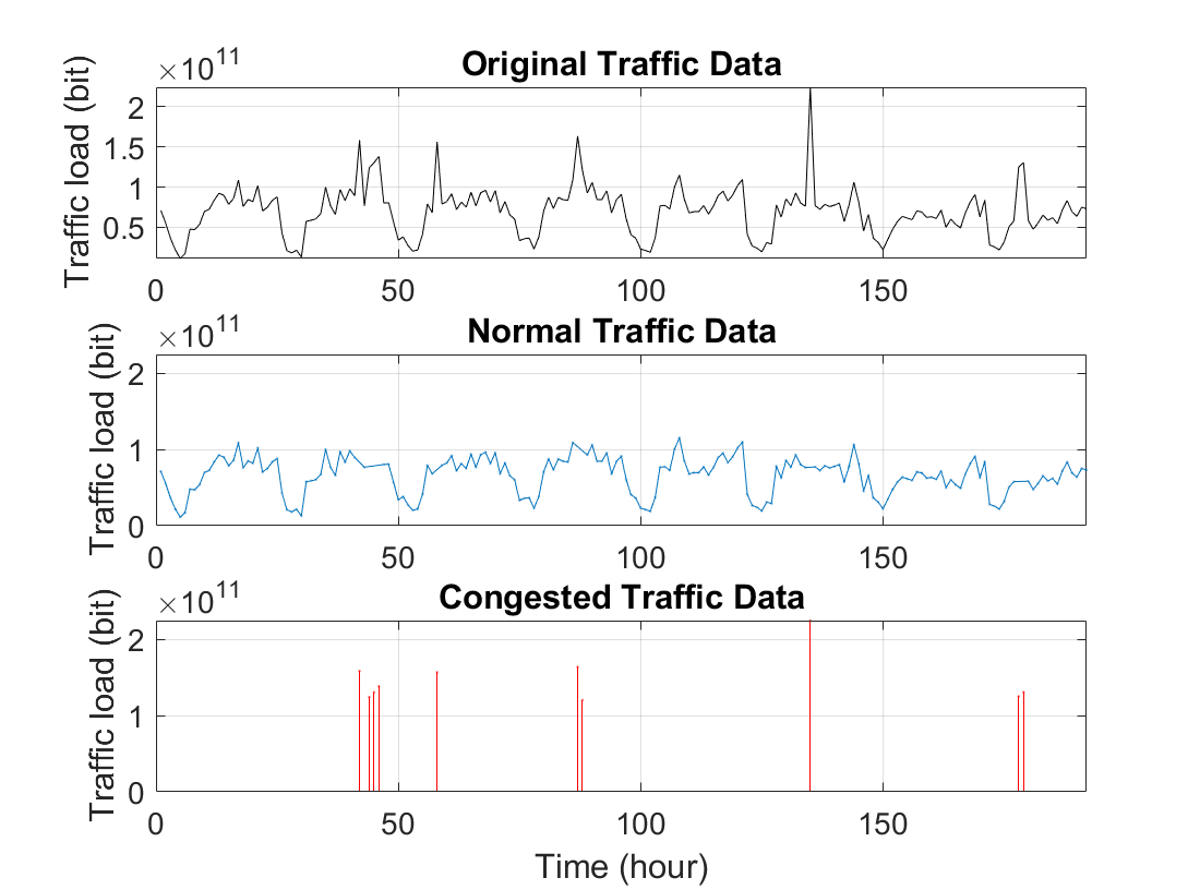
An open-source dataset “city-cellular-traffic-map” in [24] is used for the modeling, training, and testing of the proposed UAV deployment framework. The dataset collects HTTP traffic data through the cellular networks during each hour within a middle-sized city of China from August 19 to August 26, 2012. The dataset consist of two parts. One lists the identification number (ID) and the location in longitude and latitude of each BS, and the other collects the number of UEs, packets and traffic data that each BS transmits to downlink UEs during each hour. In order to identify hotspot events in the dataset, we apply the discrete wavelet transform (DWT) to the hourly cellular traffic in the city level. As shown in the upper figure of Fig. 3, the cellular traffic within the city area presents a conspicuously periodic pattern, with several sudden and erratic surges. DWT processes the time-serial data by analyzing both the value and frequency components, where the lower-frequency component defines the long term trend, and the higher-frequency component represents the small-scale rapid variation. A hotspot event usually causes a steep surge in the traffic amount. Therefore, such rapid change can be captured by DWT in the higher frequency domain. As shown in Fig. 3(a), a two-level DWT is applied to detect the frequency change of cellular traffic, and the gray bars mark the time points when the traffic amount has a sudden increase. Based on the result, the dataset is separated into the normal traffic data and the potential congested traffic, as given in Fig. 3(b). Here, we find a time window from to , which is 18 to 23 p.m. on August 20, that shows a continuously high cellular traffic amount, and the hotspot event is highly likely to happen during this period. Therefore, the traffic data from 42 to 47 are used for the predictive UAV deployment in the following analysis.
However, the data in [24] does not include the location information of each UE, or the service area of each BS. To identify the UE distribution and the traffic density, the location and time labels are generated and attached to each transmission record via the following approach. First, the service area of each BS is partitioned, based on the closest-distance principle. Next, we use the total packet number to denote the number of downlink transmissions. Furthermore, we note that the original time label in [24] is based on one hour, which is too coarse to enable our analysis. To extract the estimated data with a desired duration, a new label with a finer time grain of one second is randomly generated and attached to each traffic record. Then, given and , we divide each hour evenly into three intervals, such that the cellular data during first two minutes of each interval is used to model the UE distribution and downlink traffic, and data from the following minutes is used to estimate the UAV’s transmission performance. Eventually, the location label of each traffic record is generated by a GMM with random parameters to which we add a zero-mean Gaussian noise with a standard deviation of three meters. With additional location and time labels, the dataset is suitable for the studied problem.
VI-C Performance of the cellular traffic prediction


Fig. 4(a) shows that over UEs receive, on average, one packet within every two minutes. Thus, the transmission record that is collected during the learning stage ( minutes) is a representative training datase. In this simulation, the proposed WEM approach is applied to predict the data demand , while the actual traffic demand is calculated by summing up the real transmission amount within . Here, the mean relative error (MRE) is the metric to evaluate the prediction performance, where . Meanwhile, we introduce the EM and -mean methods as baselines. First, the EM method has been used in Section IV-A for modeling the UE distribution . Here, to predict the traffic demand using the EM method, we have , where is the time-average data rate of all UEs, and is the percentage of UEs within the hotspot area. Note that, this is a commonly-used approach to estimate cellular data demand using the UE distribution and the average rate requirement per UE in the cellular network [6]. The -mean method predicts the traffic density by averaging the local traffic density from closest neighbors.
Fig. 4(b) shows the prediction MRE of the WEM, EM, and -mean methods, where , and , as the average data demand of the hotspot UEs increases. Note that, is the average data rate per UE within the hotspot area, and is the average rate demand of all UEs within the cellular network. When , each hotspot UE will have the same data demand as the other UEs. In this case, the WEM and EM approaches yield a similar prediction accuracy with an MRE of , and the prediction errors of -mean methods are between and . Note that, a prediction error of yields lower than W of deviation on the value of . Clearly, this is a very small value compared to the hovering and transmit powers of a typical UAV. When the traffic load within different regions of the cellular network becomes more uneven, the prediction error of WEM remains the same, while the errors of the EM and -mean methods gradually increase above . Clearly, for , the proposed WEM approach outperforms all other baselines.
In the WEM approach, the traffic density of each location is considered when optimizing the prediction parameters. Therefore, the spatial feature of downlink transmissions can be accurately captured, and the performance of WEM does not decrease when the traffic load in the cellular system becomes uneven. However, the EM model only considers the location information, but ignores the downlink rate of each transmission. Therefore, when the traffic demand shows distinct patterns in different regions, the EM method fails to capture the spatial diversity, and its prediction error increases significantly. Given that the -mean method predicts the cellular traffic by averaging data from closest neighbors, it captures the traffic spatial difference from local information. However, as the cellular traffic becomes more uneven, the local information is more sensitive to the noise, and thus, the prediction errors of -mean methods increase, as increases. By comparing different -mean algorithms, we find that -mean achieves the worst performance, because information from three neighbors is not sufficient to cancel out the noise. The simulation results also show that -mean yields the best performance among all -mean methods.
VI-D The Impact of the UAV type on the utilities


In this section, we investigate the impact of the UAV type on the utilities. The contract is designed based on Lemma 1 by a BS with ID 7939, using the data from time in [24]. Fig. 5(a) shows the relationship between the UAV type and the reward, cost, as well as the overall utilities of the requesting BS and the deployed UAV, respectively. First, as the UAV type becomes larger, the BS’s reward from the downlink UEs will decrease. Although the transmit power becomes higher given a larger , a UAV with a higher type must travel for a longer time before its service. Thus, the downlink data transmission of the UAV becomes lower for a larger . Meanwhile, based on (8), we have . Therefore, a higher UAV type leads to a lower BS’s reward. Furthermore, a higher UAV type increases the payment from BS to UAV , and, thus, the utility of BS will be lower. For the deployed UAV , a larger results in a higher reward from BS , and the increase of the UAV’s reward is faster than the energy cost. Therefore, as shown in Fig. 5(a), the utility of the deployed UAV will increase, as its type becomes larger. Meanwhile, Fig. 5(a) shows that the UAV’s utility is always non-negative. Therefore, the IR condition holds in the designed contract. Fig. 5(b) investigates the impact of the contract type on the UAV’s utility. The utilities of three UAVs, where their actual types are (type-1), (type-1.25), and (type-1.5), is given, when they accept different kinds of contracts from BS 7939. As shown in Fig. 5(b), the maximum utility of each UAV is achieved when the accepted contract is of its own type. Thus, simulation results show that the IC condition holds in the designed contract set.
An interesting observation on the utility function is that the prediction error of does not cause small fluctuations on the utility value of the BS or the employed UAV. Given the transmit power as and the total payment from BS to UAV as , no longer appears in the utility formulas, and, thus, an inaccuracy in will not impact the utility functions in (9) and (10). The main effect of in the predictive UAV deployment is to determine the minimum required transmit power . If the predicted demand is much lower than the real data demand, then will be smaller. In consequence, some UAVs without enough energy may be inappropriately considered to be a qualified choice, and might be employed. On the other hand, if is much higher than the actual demand, some qualified UAVs with enough power may be excluded from the candidate set . Both cases can lead to a suboptimal solution to (12). However, as long as the error on causes no change to the association result, the utilities of the BS and UAV will always be accurate. Based on this observation, the proposed approach is highly robust to prediction errors.
VI-E Evaluation of the predictive UAV deployment
In this section, we evaluate the performance of the proposed UAV deployment method with four metrics, which are the downlink capacity, energy consumption, service delay of the employed UAVs, and the utilities of the BS and UAV operators. Meanwhile, for comparison purposes, an event-driven deployment of the closest UAV and an event-driven deployment of a UAV with the maximal on-board energy are introduced as two baselines. In both baseline approaches, the target UAV is requested by the overloaded BS and deployed, after the downlink congestion occurs, without the prediction on traffic demand. The optimal location of the deployed UAV is determined after the UAV arrives at the service area, so as to maximize its downlink transmission rate [11]. Meanwhile, in both baseline approaches, there is no contract design to determine the cost and payment between the BS to its employed UAV. Instead, the employed UAV provides the downlink service to the best of its power ability, where , and the unit payment from BS to the employed UAV is a fixed price , which equals to the unit payment from the UEs to the BS per bit of data service.


In Fig. 6, we compare the performance of the proposed predictive UAV deployment with two baselines, in terms of the total downlink capacity, average energy consumption, and average service delay of the employed UAVs. First, in Fig. 6(a), as the number of UAVs within the cellular network increases, the total downlink capacity that the employed UAVs provide to the downlink UEs increases in all three schemes. For a larger number of UAVs, the average movement distance between each overloaded BS and its employed UAV will decrease. Therefore, less energy is consumed during the mobility stage, and more power can be reserved for the downlink transmission service. In consequence, the downlink capacity of all three methods increases. However, in the closest-UAV approach, without the data demand prediction, the deployed closest UAV may not have enough on-board energy to satisfy the downlink data demand. Therefore, the downlink capacity in the closest-UAV baseline is lower than the proposed approach. In the max-energy deployment, the distance between the employed UAV and the service area is usually larger, compared to two other methods. Although the employed UAV has the largest amount of available onboard energy, due to a longer travel distance, most of the onboard energy will be consumed on mobility, and the transmit power may be insufficient. Thus, the max-energy deployment yields the lowest capacity performance among all three schemes. Moreover, the proposed approach improves the downlink capacity by over four-fold and five-fold, compared to the closest-UAV and the max-energy baselines, respectively.
Fig. 6(b) and Fig. 6(c) show the average energy consumption and service delay of each employed UAV, respectively, as the number of available UAVs in the network increases. First, we can see that the closest-UAV scheme yields the least energy cost and service delay, due to its shortest movement distance. In the proposed approach, the energy consumption and movement duration are relatively higher, because the selection criteria balances between the distance of the UAV (which determines the movement energy) and the availability of sufficient on-board energy to meet the predicted data demand. Meanwhile, the max-energy deployment results in the highest energy and time cost, due to the largest travel distance during the mobility stage. Next, for a higher number of UAVs, the energy consumption and service delay of the proposed method both drop, while the performance of the baselines remains nearly constant. In particular, as the number of UAVs increases, the performance of the proposed approach improves exponentially, and the gap between the proposed approach and the closest-UAV scheme becomes much smaller. In the proposed method, having more UAVs reduces the average distance between any employed UAV and its service point, and, hence, decreases the energy and time cost. However, in the two baselines, the number of available UAVs does not effect the travel distance during mobility. Thus, the energy consumption and service delay of two baselines remain nearly constant with the increase in the number of UAVs.
In Fig. 7, we compared the utilities of the BS and UAV operators in three schemes. First, in Fig. 7(a), for a larger number of UAVs, the average utility per BS increases in all three schemes, and the proposed approach yields the highest utility. In the proposed method, by having more UAVs, the average distance between an employed UAV to its service becomes smaller, and, thus, the type of the employed UAV with respect to the requesting BS decreases, which yields a higher utility of BS . For the closest-UAV and max-energy schemes, since the employed UAV cannot always satisfy the data demand of its downlink UEs, the utilities of each BS for both baselines are lower, compared the proposed method.
In Fig. 7(b), we can see that, as the number of UAVs increases, the total utility of the employed UAVs becomes higher in the proposed approach, while the UAVs’ utilities resulting from both baseline schemes are much lower than the proposed method. As shown in Figs. 6(a) and 6(b), by having more UAVs, the average energy cost per UAV resulting from the proposed approach will decrease, while the downlink transmission capacity of the UAV networks increases, which yields a higher income. As a result, the overall utility of the UAV operator in the proposed method will become higher for a larger number of UAVs. For the closest-UAV scheme, its lower energy consumption and shorter service delay yield a smaller deployment cost, compared with the proposed method. However, the lower downlink capacity results in less payment from the BS. Thus, the total utility of the UAV operator in the closest-UAV scheme is less than the proposed method. Moreover, based on Figs. 6(a), 6(b), and 6(c), we can see that the max-energy scheme yields the lowest transmission rate, the highest energy cost, and the longest service delay. Therefore, the utility of the UAV operators in the max-energy scheme is the lowest among all three methods. In consequence, based on Fig. 4 and Fig. 5, we can conclude that the proposed method enables an efficient UAV deployment to alleviate communication congestion in the cellular networks, and shows a significant advantage on the economical revenues of both the BS and UAV operators, compared with two baseline, event-driven approaches.


VII Conclusion
In this paper, we have proposed a novel approach for predictive deployment of UAVs to complement the ground cellular system in face of the hotspot events. In particular, four inter-related and sequential stages have been proposed to enable the ground BS to optimally employ a UAV to offload the excess traffic. First, a novel framework, based on the EM and WEM methods, has been proposed to estimate the UE distribution and the downlink traffic demand. Next, to guarantee a truthful information exchange between the BS and UAV operators, a traffic offload contract have been developed, and the sufficient and necessary conditions for having a feasible contract have been analytically derived. Then, an optimization problem have been formulated to deploy the optimal UAV onto the hotspot area in a way that the utility of each overloaded ground BS is maximized. Simulation results show that the proposed WEM approach yields a prediction error around , and compared with the EM and -mean schemes, the WEM algorithm yields a higher prediction accuracy, particularly when the traffic load in the cellular system becomes spatially uneven. Furthermore, compared with two event-driven schemes based on the closest-distance and maximal-energy metrics, the proposed predictive deployment approach enables UAV operators to provide efficient downlink service for hotspot users, and significantly improves the revenues of both the BS and UAV networks.
Appendix A Proof of Proposition 1
We first use contradiction to prove the proposition that if , then . Suppose that there exists , but . Then, we have
| (20) |
On the other hand, from IC condition, we have
| (21) |
By adding the inequations in (21), we have , which contradicts to (20). This completes the first part of the proof.
Next, we prove that if , . From the IC condition, we have , i.e. . Since , we conclude , and thus . This completes the proof.
Appendix B Proof of Theorem 1
For notation simplicity, in this section, we denote , , , as , , , respectively.
B-A Proof for necessary conditions
Given the IR and IC conditions, we prove Theorem 1 in this section. First, as shown in Proposition 1, for any , once , then and . Therefore, condition (a) of Theorem 1 is proved by Proposition 1. Second, condition (b) of Theorem 1 is supported by the IR condition, where for all in , which naturally includes . Next, we prove condition (c). Let . According to the IC condition, for any , we have: , i.e., . If , then according to Proposition 1, and . Here, we exclude the situation where and in the following discussion of this proof, because condition (c) naturally holds in this case. Therefore, for any , we have
| (22) |
If , then and . Thus, for any ,
| (23) |
Combing (22) and (23), we have , which proves condition (c) of Theorem 1.
B-B Proof for sufficient conditions
From Theorem 1, we will prove the IR and IC conditions in this section. First, we prove the IR condition. According to condition (b) of Theorem 1, satisfies the IR condition. Then, we prove that for any , the IR condition holds. From condition (c) of Theorem 1, we have the following inequalities, , i.e.,
| (24) |
From condition (b), we have
| (25) |
By combing (24) and (25), we have . Thus, for any , the IR condition holds.
In the end, we prove the IC condition. Let . And we prove that . From condition (c), we have, if , then . i.e., . Therefore, . On the other hand, if , then . i.e., . Therefore, . Consequently, the IC condition holds.
References
- [1] Q. Zhang, M. Mozaffari, W. Saad, M. Bennis, and M. Debbah, “Machine learning for predictive on-demand deployment of UAVs for wireless communications,” in Proc. of IEEE Global Communications Conference, Abu Dhabi, UAE, Dec 2018.
- [2] M. Mozaffari, W. Saad, M. Bennis, and M. Debbah, “Mobile unmanned aerial vehicles (UAVs) for energy-efficient Internet of Tshings communications,” IEEE Transactions on Wireless Communications, vol. 16, no. 11, pp. 7574–7589, Sep 2017.
- [3] R. I. Bor-Yaliniz, A. El-Keyi, and H. Yanikomeroglu, “Efficient 3-D placement of an aerial base station in next generation cellular networks,” in Proc. of IEEE International Conference on Communications, Kuala Lumpur, Malaysia, May 2016.
- [4] X. Zhang and L. Duan, “Fast deployment of UAV networks for optimal wireless coverage,” IEEE Transactions on Mobile Computing, vol. 18, no. 3, pp. 588–601, May 2018.
- [5] W. Khawaja, I. Guvenc, D. Matolak, U.-C. Fiebig, and N. Schneckenberger, “A survey of air-to-ground propagation channel modeling for unmanned aerial vehicles,” IEEE Communications Surveys and Tutorials (Early Access), May 2019.
- [6] M. Mozaffari, W. Saad, M. Bennis, Y.-H. Nam, and M. Debbah, “A tutorial on UAVs for wireless networks: Applications, challenges, and open problems,” IEEE Communications Surveys and Tutorials, vol. 21, no. 4, pp. 3039–3071, Fourth quarter 2019.
- [7] M. Mozaffari, A. T. Z. Kasgari, W. Saad, M. Bennis, and M. Debbah, “Beyond 5G with UAVs: Foundations of a 3D wireless cellular network,” IEEE Transactions on Wireless Communications, vol. 18, no. 1, pp. 357–372, Jan 2018.
- [8] W. Saad, M. Bennis, and M. Chen, “A vision of 6G wireless systems: Applications, trends, technologies, and open research problems,” IEEE Network, to appear, 2020.
- [9] M. Chen, U. Challita, W. Saad, C. Yin, and M. Debbah, “Artificial neural networks-based machine learning for wireless networks: A tutorial,” IEEE Communications Surveys and Tutorials, to appear, 2019.
- [10] Z. Hu, Z. Zheng, L. Song, T. Wang, and X. Li, “UAV offloading: Spectrum trading contract design for UAV assisted cellular networks,” IEEE Transactions on Wireless Communications, vol. 17, no. 9, pp. 6093–6107, July 2018.
- [11] M. Mozaffari, W. Saad, M. Bennis, and M. Debbah, “Optimal transport theory for power-efficient deployment of unmanned aerial vehicles,” in Proc. of IEEE International Conference on Communications, Kuala Lumpur, Malaysia, May 2016.
- [12] E. Kalantari, H. Yanikomeroglu, and A. Yongacoglu, “On the number and 3D placement of drone base stations in wireless cellular networks,” in Proc. of IEEE 84th Vehicular Technology Conference, Montreal, QC, Canada, Sep 2016.
- [13] J. Lyu, Y. Zeng, and R. Zhang, “UAV-aided offloading for cellular hotspot,” IEEE Transactions on Wireless Communications, vol. 17, no. 6, pp. 3988–4001, Mar 2018.
- [14] V. Sharma, M. Bennis, and R. Kumar, “UAV-assisted heterogeneous networks for capacity enhancement,” IEEE Communications Letters, vol. 20, no. 6, pp. 1207–1210, Apr 2016.
- [15] J. Lyu, Y. Zeng, and R. Zhang, “Spectrum sharing and cyclical multiple access in UAV-aided cellular offloading,” in Proc. of IEEE Global Communications Conference, Singapore, Dec 2017.
- [16] F. Cheng, S. Zhang, Z. Li, Y. Chen, N. Zhao, R. Yu, and V. C. Leung, “UAV trajectory optimization for data offloading at the edge of multiple cells,” IEEE Transactions on Vehicular Technology, vol. 67, no. 7, pp. 6732 – 6736, Mar 2018.
- [17] S. Sharafeddine and R. Islambouli, “On-demand deployment of multiple aerial base stations for traffic offloading and network recovery,” Computer Networks, vol. 156, pp. 52–61, June 2019.
- [18] R. Li, Z. Zhao, J. Zheng, C. Mei, Y. Cai, and H. Zhang, “The learning and prediction of application-level traffic data in cellular networks,” IEEE Transactions on Wireless Communications, vol. 16, no. 6, pp. 3899–3912, Mar 2017.
- [19] C. Yu, Y. Liu, D. Yao, L. T. Yang, H. Jin, H. Chen, and Q. Ding, “Modeling user activity patterns for next-place prediction,” IEEE Systems Journal, vol. 11, no. 2, pp. 1060–1071, July 2017.
- [20] P. Valente Klaine, M. A. Imran, O. Onireti, and R. D. Souza, “A survey of machine learning techniques applied to self organizing cellular networks,” IEEE Communications Surveys and Tutorials, vol. 19, no. 4, pp. 2392–2431, July 2017.
- [21] M. Chen, W. Saad, and C. Yin, “Liquid state machine learning for resource and cache management in LTE-U unmanned aerial vehicle (UAV) networks,” IEEE Transactions on Wireless Communications, vol. 18, no. 3, pp. 1504 –1517, Jan 2019.
- [22] J. Chen, U. Yatnalli, and D. Gesbert, “Learning radio maps for UAV-aided wireless networks: A segmented regression approach,” in Proc. of IEEE International Conference on Communications, Paris, France, May 2017.
- [23] R. Amorim, J. Wigard, H. Nguyen, I. Z. Kovacs, and P. Mogensen, “Machine-learning identification of airborne UAV-UEs based on LTE radio measurements,” in Proc. of IEEE Globecom Workshops, Singapore, Jan 2017.
- [24] “City cellular traffic map,” https://github.com/caesar0301/city-cellular-traffic-map, accessed: 2016-10-05.
- [25] P. Bolton and M. Dewatripont, Contract theory. MIT press, 2005.
- [26] L. Zhu, J. Zhang, Z. Xiao, X. Cao, D. O. Wu, and X.-G. Xia, “3D beamforming for flexible coverage in millimeter-wave uav communications,” IEEE Wireless Communications Letters, 2019.
- [27] A. Al-Hourani, S. Kandeepan, and A. Jamalipour, “Modeling air-to-ground path loss for low altitude platforms in urban environments,” in Proc. of IEEE Global Communications Conference, Austin, TX, USA, Dec 2014.
- [28] A. Al-Hourani, S. Kandeepan, and S. Lardner, “Optimal LAP altitude for maximum coverage,” IEEE Wireless Communications Letters, vol. 3, no. 6, pp. 569–572, July 2014.
- [29] J. Lyu, Y. Zeng, and R. Zhang, “Cyclical multiple access in UAV-aided communications: A throughput-delay tradeoff,” IEEE Wireless Communications Letters, vol. 5, no. 6, pp. 600–603, Aug 2016.
- [30] Y. Zeng, J. Xu, and R. Zhang, “Energy minimization for wireless communication with rotary-wing UAV,” IEEE Transactions on Wireless Communications, vol. 18, no. 4, pp. 2329 – 2345, 2019.
- [31] A. T. Z. Kasgari, W. Saad, and M. Debbah, “Human-in-the-loop wireless communications: Machine learning and brain-aware resource management,” IEEE Transactions on Communications, to appear, 2019.
- [32] B. Selim, O. Alhussein, S. Muhaidat, G. K. Karagiannidis, and J. Liang, “Modeling and analysis of wireless channels via the mixture of Gaussian distribution,” IEEE Transactions on Vehicular Technology, vol. 65, no. 10, pp. 8309–8321, 2015.
- [33] M. B. Christopher, Pattern recognition and machine learning. Springer-Verlag New York, 2016.
- [34] “DJI matrice 200 series v2 specifications,” https://www.dji.com/downloads/products/matrice-200-series-v2, accessed: 2019.