Bayesian Hierarchical Modeling on Covariance Valued Data
Abstract : Analysis of structural and functional connectivity (FC) of human brains is of pivotal importance for diagnosis of cognitive ability. The Human Connectome Project (HCP) provides an excellent source of neural data across different regions of interest (ROIs) of the living human brain. Individual specific data were available from an existing analysis (Dai et al., 2017) in the form of time varying covariance matrices representing the brain activity as the subjects perform a specific task. As a preliminary objective of studying the heterogeneity of brain connectomics across the population, we develop a probabilistic model for a sample of covariance matrices using a scaled Wishart distribution. We stress here that our data units are available in the form of covariance matrices, and we use the Wishart distribution to create our likelihood function rather than its more common usage as a prior on covariance matrices. Based on empirical explorations suggesting the data matrices to have low effective rank, we further model the center of the Wishart distribution using an orthogonal factor model type decomposition. We encourage shrinkage towards a low rank structure through a novel shrinkage prior and discuss strategies to sample from the posterior distribution using a combination of Gibbs and slice sampling. The efficacy of the approach is explored in various simulation settings and exemplified on several case studies including our motivating HCP data. We extend our modeling framework to a dynamic setting to detect change points.
Keywords: change point, covariance matrix, functional connectivity, low rank, Stiefel manifold, Wishart distribution
1 Introduction
Functional connectomes play a critical role in determining how the brain responds to everyday tasks and life’s challenges (Park and Friston, 2013; Glasser et al., 2016a; Jbabdi et al., 2015). In recent years, there has been an abundance of literature focusing on understanding the variation of functional connectomes in healthy and diseased people and their relationships to various covariates and phenotypes (Smith et al., 2015; Finn et al., 2015; Zhang et al., 2018). Such interests are inspired and propelled by large scale neuroimaging studies, such as the Human Connectome Project (HCP) (Van Essen et al., 2013; Glasser et al., 2016b), the Alzheimer’s Disease Neuroimaging Initiative (ADNI) (Weiner et al., 2010) and the UK Biobank (Miller et al., 2016). In this article, we focus our attention to functional connectome (FC) inferred from functional magnetic resonance imaging (fMRI) data that measures the blood oxygen level dependent (BOLD) contrast signals of each brain voxel. As opposed to the anatomical axon connections (also referred as structural connectome), FC quantifies functional dependences between brain regions through correlations or covariances of BOLD signals. Conventional FC is often represented as a covariance or correlation matrix of fMRI data over a long recording time (Friston, 2011; Hutchison et al., 2013), where the matrix size equals the number of ROIs being considered.
While FC is assumed to be fixed or static over time in earlier studies, there is an abundance of evidence (Hutchison et al., 2013; Monti et al., 2014; Hindriks et al., 2016) in recent studies showing that FC is a dynamic process. The dynamic FC (dFC) is represented as a time series of short-term FCs which are calculated using functional MRI data over small time intervals. Due to limitations of the fMRI BOLD (blood oxygen level dependent) contrast signals, fMRI signals are not directly analyzed (Glover, 2011; Turner, 2016). The most popular way to transfer BOLD signals into something that is reasonable to analyze is to calculate coherence between different brain regions, e.g., correlation or covariance. We choose to use the covariance matrix, which in general carries more information than the correlation matrix. The goal of this paper is to understand and infer on the structure of dFC and detect change points in the dFC as the subjects perform a specific action. We first model the short-term FC using a scaled Wishart distribution and then generalize the static model to a hierarchical model of a time series of covariance matrices. Our final goal is to detect and compare individual specific change points along the dFC based on this hierarchical model.
As argued before, a first step towards change point detection is to model a population of covariance matrices. This is entirely different from covariance matrix estimation from multivariate data, which is a well-studied problem; see (Leonard et al., 1992; Daniels and Kass, 1999; Pati et al., 2014) as some representative examples of Bayesian inference for covariance matrices and (Pourahmadi, 2011) for a more comprehensive review. In the covariance estimation context, the observational data vectors are directly available and the goal is to characterize the dependence amongst the different variables in the data from multiple independent and identically distributed samples. On the other hand, our observational units are covariance matrices corresponding to different individuals observed over time, which we shall henceforth refer to as covariance-valued data. Hierarchical models for capturing heterogeneity in multiple related groups based on covariance matrices are relatively fewer in number (Flury, 1984; Flury, 1987; Boik, 2002; Franks and Hoff, 2019; Hoff, 2009a). Schott, 1999; Schott, 2001 developed hypothesis testing methods based on covariance structures. In a Bayesian context, Daniels, 2006; Pourahmadi et al., 2007; Barnard et al., 2000 considered parsimonious modeling of covariance matrices, which were extended to a longitudinal setting by Gaskins and Daniels, 2013; Das and Daniels, 2014; Gaskins et al., 2014; Gaskins and Daniels, 2016. A parallel sequence of works proposes modeling of fMRI data-matrices via Gaussian graphical modeling techniques (Stingo et al., 2013; Warnick et al., 2018). In contrast to the existing studies, we built a hierarchical model on observed covariance valued datasets to detect individual specific change points. The literature on probabilistic modeling for covariance-valued data in the time series context (Golosnoy et al., 2012; Gouriéroux et al., 2009; Yu et al., 2017) is focused on maximum likelihood estimation using a non-central Wishart distribution as the likelihood. For example, the dataset considered in Yu et al., 2017 comprises of low-dimensional (5 by 5) daily realized covariance (RCOV) matrices for 5 stocks observed across 2274 time points. This single time series sequence is modeled using a generalized conditional autoregressive Wishart (GCAW) model. In presence of smaller number of parameters and a huge collection of time points, maximum likelihood estimation is a natural choice for model fitting. On the other hand, since we are dealing with 10 by 10 covariance matrices observed over 26 time points for 500 individuals, it is important to borrow information across individuals and seek for a parsimonious modeling framework.
To that end, we develop a suite of hierarchical modeling techniques for covariance-valued data to provide insight into the structural connectivity of human brains. We use a scaled version of the Wishart distribution to model the covariance-valued observations. While the Wishart distribution is commonly used as a prior distribution on inverse-covariance or precision matrices in Bayesian inference, its usage as a likelihood is novel in the Bayesian context to best of our knowledge. The presence of a modest number of observations further necessitates structured modeling of the center of the Wishart distribution, which itself is a covariance matrix. Based on empirical evidence of low effective ranks of the data matrices, we modeled the center of the Wishart model using an orthogonal factor model type decomposition and encouraged shrinkage towards a low rank structure through the development of a novel shrinkage prior. We use a combination of Gibbs and slice sampling to sample from the posterior distribution whose steps are mostly standard.
Our primary objective is to explore the dynamic nature of FC between different brain regions during performances of certain tasks. A dynamical FC model provides an overall architecture of how the brain functions as the individual perform certain tasks. An important scientific goal is to identify change points (Barry and Hartigan, 1993) in the time series of covariances that split the data into contiguous segments. Difference in the change points across individuals are indicative of behavioral and cognitive differences (Dai et al., 2017). To address this, we extend our hierarchical model to accommodate a single or multiple change points in a fully Bayesian framework. A novel combination of existing MCMC algorithms renders sampling from the joint posterior distribution tractable. The change point model is then implemented on both the HCP and the ADNI datasets to extract scientifically meaningful conclusions. For the HCP dataset, we studied the change point pattern during the motor task and discovered the primary FC change point occurs when people switch the movement from hand and foot to the tongue. For the ADNI dataset, we compared FCs in two groups of older people (supernormal subjects and normal controls) and found that supernormal subjects have higher strength of connectivity within posterior regions or between posterior and anterior regions of their brain.
In this paper, we begin with an illustration of our motivating data set in section 2 followed by a model for covariance matrices (section 3.1), hierarchical covariance model (section 3.2) and hierarchical change point model (section 4). Results of detailed simulation study are provided for each of the three models. In section 5, we provide the results obtained from our motivating HCP dataset under hierarchical change point model followed by model validation in section 6. We studied a dynamic extension of our hierarchical model in Appendix (section A). Section B in Appendix contains some additional results on sensitivity and robustness analysis of the hierarchical change point model.
2 Data description
We utilize functional MRI data from two large datasets, ADNI (Weiner et al., 2010) and HCP (Van Essen et al., 2013) to illustrate the proposed method. ADNI was initiated by National Institute on Aging, the National Institute of Biomedical Imaging and Bioengineering, the Food and Drug Administration, and some private pharmaceutical companies and non-profit organizations. ADNI assesses clinical, imaging, genetic and bio specimen biomarkers through the process of normal aging to early mild cognitive impairment, to late mild cognitive impairment, to dementia or Alzheimer’s disease (AD). Participants were recruited across North America to participant in three phases of the study: ADNI1, ADNI GO and ADNI2. A variety of imaging and clinical assessments were conducted for each participant. Results were then shared by ADNI through the Laboratory of Neuro Imaging’s Image Data Archive (https://ida.loni.usc.edu/). In our study, we focus on a subset of healthy subjects that were previously identified in (Lin et al., 2017a). These subjects were AD free but were clustered in two groups. The first group is called supernormals who exhibited excellent episodic memory and executive function. The other group is age-matched healthy control subjects. All their resting-state fMRI data were collected using a 3.0 Tesla Phillips MRI with an echo-planar imaging sequence (spatial resolution = mm3). Structural images were obtained using an MPRAGE sequence (spatial resolution mm3), which were then used for registration during preprocessing. Across individuals, the first 10 volumes were discarded to avoid potential noise related to the equilibrium of the scanner and participant’s adaptation process. The remaining 130 volumes were preprocessed using slice time correction and head motion correction. The images were then registered to each individual’s own structural image, normalized to the Montreal Neurological Institute (MNI) standard space and spatially smoothed using a Gaussian kernel (FWHM = 4 mm). We utilized the automated anatomical labeling (AAL) (Tzourio-Mazoyer et al., 2002) to percolate the whole brain into regions of interest (ROIs).
The HCP project aims at characterizing human brain connectivity in healthy adults and to enable detailed comparisons between brain circuits, behavior and genetics at the level of individual subjects. The HCP raw and preprocessed data can be easily accessed through ConnectomeDB (http://www.humanconnectome.org). The high-quality imaging data and the easy accessibility make it an ideal dataset for this paper. Majority of the HCP fMRI data were acquired at 3T with a mm3 resolution. Preprocessing steps using the HCP pipeline (Glasser et al., 2013; Glasser et al., 2016b) were performed before any data analysis, e.g., removing spatial distortions, realigning volume to compensate for subject motion, registering the fMRI to the structural MRI, reducing the bias field, normalizing the 4D image to a global mean, masking the data with the final brain mask and aligning the brain to a standard space. Figure 1 provides an overview of the preprocessing steps.

The Destrieux atlas (Destrieux et al., 2010) was used to percolate cortical regions into 74 nodes per hemisphere. Similar to Dai et al., 2017, for the fMRI BOLD signal in each ROI, we first calculate a mean time series, and then we utilize a sliding window method to calculate a covariance trajectory for subject at -th window based on selected ROIs. Therefore, is a covariance matrix representing the short time functional connectome, where p denotes number of ROIs.
3 Hierarchical Modeling for Covariance Dataset
Since the covariance matrices are observed for multiple individuals and time points, a natural course of action is to build a parsimonious model that borrows strength across all observational units. We first discuss an independence model with scaled Wishart distribution for covariance-valued data that serves as the basic building block for the forthcoming extensions. Both the central and non-central Wishart distributions have full support on the space of covariance matrices. However, the non-central Wishart distribution has more parameters making prior elicitation more complicated. Moreover, the presence of key parameters inside a hypergeometric function complicates posterior computation; in particular, the nice conjugate structure that we exploit throughout the article is lost. Due to these reasons, we consider a central Wishart likelihood through the rest of the paper.
Motivated by a pattern we observe in the functional connectivity data, the mean structure of the independence model is encouraged to shrink towards low rank matrices via a parsimonious shrinkage prior. We develop an MCMC algorithm to fit the independence model to data and show its efficacy in a simulation study. Next, the independence model is extended to a Bayesian hierarchical model to incorporate multiple individuals, allowing for subject specific deviations from a common mean structure. Fitting the hierarchical model requires sampling from a class of distributions on the Stiefel manifold which can be done efficiently using the algorithm in §3.3 of Hoff, 2009b; refer to §3.2 herein for more details. The hierarchical model leads to our eventual goal of detecting subject specific change points in the functional connectivity data.
3.1 Independence Model
We begin by describing the details of the independence model. Let be a collection of independent and identically distributed covariance matrices. We probabilistically model the s using a Wishart distribution, which is arguably the most recognized distributional family for covariance matrices. We shall use the standard notation to denote the Wishart distribution on the space of positive definite matrices, with degrees of freedom and a positive definite scale matrix . The density distribution has a density (in ) proportional to
Specifically, we use a scaled Wishart distribution to model the s,
| (1) |
The introduction of the parameter in the scale matrix is to decouple its presence in both the mean and covariance. For , one has
whereas for ,
Thus, in the parameterization we work with, is the population mean. We henceforth fix at and validate our assumption in Appendix D. Now, we focus our attention on modeling the mean .
An unstructured covariance matrix has free elements, (e.g. in the HCP dataset, leading to a total number of parameters and in the ADNI dataset, in the present case leading to parameters). Given that we only have a modest number of time points, it is important to make meaningful structural assumptions on to reduce the effective number of parameters to be estimated. We conducted an exploratory analysis to find patterns in the data matrices that could direct us towards a parsimonious model. The data matrices and their inverses did not contain any obvious sparsity pattern. Next, we investigated the effective ranks of the data matrices. For a positive definite matrix with eigenvalues , its effective or intrinsic rank (Vershynin, 2012),
is the ratio of its trace and largest eigenvalue. The effective rank satisfies , so that it always provides a lower bound to the actual rank. Further, the effective rank is a smooth function of its argument. For example, consider the class of matrices
for and a -dimensional vector of unit length. The matrices increasingly get close to being rank deficient as , however, this is not captured by the rank as for any . On the other hand, , which smoothly decays to as . These features render the effective rank a suitable measure to capture the intrinsic dimensionality of a matrix and indicate potential near rank-deficiencies.

Figure 2 shows boxplots of the effective ranks of the data matrices across the 26 time points for 50 randomly selected individuals from motor task of HCP dataset. It is evident that the data matrices have low effective rank, with the bulk of the empirical effective rank distribution between and . This observation motivated us to consider an orthogonal factor model type decomposition (Hoff, 2009a) for to exploit the near low-rank structure as
| (2) |
where for some is a semi-orthogonal matrix satisfying , and is a diagonal matrix with non-negative diagonal entries. Such a decomposition readily satisfies the positive definiteness constraint on . Different variance components are typically employed in factor analysis to account for variables may with different scales. However, since all the entries represent functional connectivities, we make the simplifying assumption of using the same for all the components.
We operate in a Bayesian framework to perform inference based on the posterior distribution of the model parameters. Before proceeding to describe our prior specifications, it is important to discuss the role of in what follows. In a fully Bayesian framework, one may treat as a parameter which designates the effective rank of and assign it a prior distribution; the discrete uniform distribution on being a default choice. Under this prior, the posterior distribution of is proportional to the marginal likelihood of the data given , which is intractable in the present context. While it is possible to sample inside a larger trans-dimensional MCMC algorithm such as the reversible jump MCMC (RJMCMC), its implementation remains computationally challenging, especially when considering extensions to the hierarchical modeling setup later on. Moreover, the effective rank does not have a clear biological interpretation in our real application and is purely a modeling device to induce parsimony. Based on these considerations, we undertake a shrinkage approach rather than explicit selection of the rank. Specifically, we set to a conservative upper bound, with being a default choice, and encourage a subset of the diagonal entries of to shrink towards zero. If denotes the active subset, that is, the subset of diagonal entries of that are left unshrunk, then , where denotes the sub-matrix of corresponding to the columns in , and denotes the corresponding diagonal sub-matrix of . This leads to an approximately low rank decomposition under the posterior, which is sufficient for our purpose. In the factor modeling context, Bhattacharya and Dunson, 2012 considered a shrinkage prior on the factor loadings matrix rather than placing a prior on the number of factors, e.g., as in Lopes and West, 2004. We have a very different shrinkage mechanism as our shrinkage operates on the diagonal matrix .
Fixing , the unknown parameters in our model are with parameter space , where denotes the Stiefel manifold of semi-orthogonal matrices, and the collection of dimensional diagonal matrices with non-negative entries. The likelihood function for the parameters is given by
| (3) |
We now discuss prior choices on the parameters. For computational convenience, we reparameterize to where , so that . We place a uniform prior on supported on the Stiefel manifold , and an inverse-gamma prior on . To set up our sparsity favoring shrinkage prior on the diagonal entries s of , first decompose
| (4) |
In (4), plays the role of a global shrinkage parameter while the s allow for coordinate specific deviations, much in the spirit of the global-local shrinkage priors popularly used in regression (Carvalho et al., 2010). We place independent half-Cauchy priors on the s, , with density proportional to . The half-Cauchy prior is a popular choice as a prior distribution of shrinkage parameters due to its positive density at zero and heavy tails (Polson and Scott, 2012; Carvalho et al., 2010). We complete the prior specification by placing a half-Cauchy prior truncated to on . Truncating the prior on the global parameter leads to better identifiability and is recommended by van der Pas et al., 2014 in the context of the horseshoe prior. The multiplicative prior on the s can also be interpreted as an additive one-way ANOVA type decomposition in the logarithmic scale,
with grand mean and main effects s. The posterior computation is also conveniently carried out in the logarithmic scale, which we describe next.
We develop a fully automated and easy to implement Markov chain Monte Carlo algorithm to sample from the joint posterior distribution of given the data. Specifically, we use a combination of Gibbs sampling with slice sampling and Metropolis-within-Gibbs to iteratively sample from the full-conditional distribution of each parameter block given the rest. The sampler iterates through the following steps; the derivations are deferred to the Appendix (section E). We use the notation to denote the full conditional distribution of a parameter.
- •
Sample from its matrix Bingham full-conditional distribution. The matrix Bingham distribution has a density with respect to the uniform distribution on the Stiefel manifold given by
where and are symmetric and diagonal matrices, respectively. In our case, is a symmetric matrix by definition and The matrix Bingham distribution is conveniently sampled using the R package rstiefel (Hoff, 2013).
- •
Update the s from their independent full conditional distributions using slice sampling. Set and consider the transformation for . Then sample
Uniform,
Gamma(shape , rate ) truncated to the region , and set . - •
To sample , propose and compute the Metropolis ratio
where denotes the full-conditional of . Accept with probability .
- •
Sample from its inverse-gamma full conditional distribution as
where .
We observed good mixing and convergence of the above MCMC sampler based on standard MCMC diagnostics. Although not our primary motivation, one can estimate the effective rank based on a simple post-processing step of the MCMC samples for the s. As in Bhattacharya et al., 2015; Li and Pati, 2017 at each MCMC iteration, we cluster the s into two groups using 2-means clustering and save the size of the group having the larger mean. The mode of these numbers across the MCMC iteration is then used as an estimate of the effective or intrinsic rank. We find that this approach performs well in our simulation and real examples. A more nuanced approach for post-processing was proposed by Li and Pati, 2017, which can also be used in the present context.
3.1.1 Simulation Study for Independence Model
We conduct a detailed simulation study to illustrate the performance of the independence model in terms of recovering the true parameters. We fixed and varied . The true intrinsic rank of the data generating mechanism was fixed at to mimic the observation in Figure 2. We set , the true , the true and considered from a uniform distribution on Stiefel manifold . 100 independent datasets have been generated from the model (1). We denote the true covariance matrix by .
For model fitting, we set ; see Section B of the Appendix for a sensitivity analysis. The inverse-gamma hyperparameters and were elicited in an empirical Bayes approach. Specifically, we used a method-of-moments type estimator for these hyperparameters. We ran our MCMC algorithm for 10,000 many iterations, discarding the first 5000 many iterates as burn-in. Letting denote an estimate of the posterior mean based on the retained MCMC samples, we provide boxplots of the scaled Frobenius norm difference across the 100 replicates for the different values of in Figure 3(a). Here, and elsewhere, denotes the Frobenius norm of a matrix. As expected, both the center and spread of the boxplots tend to decrease with increasing , implying the consistency of the posterior mean in recovering the population mean. Figure 3(b) shows density plots of the posterior samples of which increasingly concentrate around the true value, , with increasing .


Next, we compare the performance of the posterior mean with the sample mean , which is an unbiased estimator of . We consider three different norms between covariance matrices (Ian L. Dryden and Zhou, 2009) listed in Table 1.
| Name | Notation | Form |
|---|---|---|
| Euclidean | ||
| Riemannian | ||
| Cholesky |
For each distance , we compare and for ; summary measures are tabulated in Table 2 and Table 3 for and respectively. We scaled the distances except the Riemannian norm by for tabulation; the Riemannian norm is scale-invariant. Boxplots of the distances (in their original scale) across the 100 replicates are provided in Figure 4. It is evident that the posterior mean overall provides a substantial improvement over the sample mean, especially in higher dimensional situations.
| Euclidean | Riemannian | Cholesky | ||||
|---|---|---|---|---|---|---|
| PM | SM | PM | SM | PM | SM | |
| Euclidean | Riemannian | Cholesky | ||||
|---|---|---|---|---|---|---|
| PM | SM | PM | SM | PM | SM | |


Finally, we illustrate the performance of the post-processing step outlined in the previous subsection to estimate the effective rank. We only consider and 2 different settings of , (i) and (ii) . Setting (ii) has a weaker signal strength compared to (i). Following the discussed methodology and setup, we provide the rank estimates under different scenarios in Figure 5 which shows high probability mass at and in Figure 5(a) and 5(b) respectively. In different simulation settings, our proposed method is able to recover the true ranks. We highlight that the simulation is performed under mild model misspecification - the true covariance matrix in our simulation study is chosen to be exactly low-rank whereas our model only assumes a near low-rank structure. Despite this, our model is able to detect the true rank.


3.2 Hierarchical Covariance Model
In this subsection, we extend the independence model to a hierarchical modeling framework encompassing all the individuals. Our hierarchical modeling framework lets the different individuals to share common parameters while allowing for subject specific deviations, striking a balance between pooling of information across different individuals while retaining flexibility. Letting denote the observed covariance matrix for individual at time , we let
| (5) |
The first line of (5) posits the same scaled Wishart model as in the previous subsection with individual specific mean . As discussed earlier, we only have data on time points for each individual. On the other hand, there are a relatively larger number of individuals in the study. For this reason, rather than separately fitting the independence model for each individual, we consider a structured decomposition of that lets and vary across individuals, while keeping fixed. This is akin to an expansion of the s in terms of a fixed dictionary , with subject specific loadings. This fixed dictionary expansion vastly reduces the number of model parameters and allows one to borrow information across individuals to estimate the common dictionary . We continue using for the residual part in the covariance decomposition for model parsimony. We later conduct model validation to show that model (5) provides an adequate fit to the data compared to separately fitting the independence model.
We continue to use the uniform prior on the Stiefel manifold for . After reparameterizing to , we place independent copies of the shrinkage prior introduced earlier on the s, and independent inverse-gamma priors on the s.
We extend the MCMC algorithm for the independence model to the hierarchical setting. The updates for and proceed independently across exactly along same lines as before. However, since is common to all individuals, its full conditional no longer remains a matrix Bingham distribution. We show in the Appendix (section F) that the full-conditional distribution of is given by
| (6) | ||||
We sample from the above density by adopting the Gibbs sampling scheme of Hoff, 2009b to sample from a class of matrix Bingham–von Mises–Fisher (BMF) distributions (Khatri and Mardia, 1977). The BMF distribution has a density on the Stiefel manifold given by . Hoff considers the case when is diagonal, noting that the general symmetric case can be handled by a transformation, when the density assumes the form
Hoff used Gibbs sampling to sample from by alternately sampling from the full-conditional distributions of each column given the rest; see § 3.3 of Hoff, 2009b for details.
3.3 Simulation study for Hierarchical Covariance Model
We conduct a replicated simulation study to illustrate the operating characteristics of the hierarchical model. We set and for our simulations. The true is generated uniformly on the Stiefel manifold. Also, for each , the diagonal entries of the true are generated uniformly between and , while the s are generated uniformly between and . We generate 100 independent simulation replicates as above.
We fit the hierarchical model using the MCMC outlined in the previous subsection. We set and use a modification of the empirical Bayes procedure to elicit the hyperparameters and . As metrics of parameter recovery, we considered
| (7) |
where and are the posterior means of and for . and is an individual specific measure of the distance of the posterior mean from the truth, while and are average measures over all the individuals.

As a point of comparison, we also fit the independence model in the previous subsection separately for each individual. Figure 6 shows boxplots of averaged over the simulation replicates for the hierarchical and independence model. The tighter spread of the boxplot for the hierarchical model indicates the gains from borrowing information across subjects. The hierarchical model also successfully recovered the true ranks as shown in Figure 8.


We conducted a second set of simulations by varying and . A summary is presented in Figure 9. In the top left panel, we provide the boxplot of across the 100 simulation replicates for the different values of keeping fixed, while the bottom left panel provides the same for varying and fixed . As expected, the estimation performance improves for larger and smaller . We observe similar pattern in the density plots of w.r.t. increasing , fixed (Figure 9(b)) and fixed , increasing (Figure 9(d)).


3.4 Real Data Analysis for ADNI dataset
In this case study, we utilize 18 subjects’ resting-state fMRI data from ADNI. Half of them are from supernormal (SN) subjects who possess excellent (Lin et al., 2017a; Lin et al., 2017b), and the other half are healthy control (HC) subjects. Each group contains 9 individuals with its resting state fMRI data at baseline preprocessed. From previous literature, we identified seven interesting ROIs, left occipital cortex, left occipital cortex, left precuneus, left superior temporal cortex, right middle frontal gyrus, right parahippocampus, right thalamus (indexed as ROI ), that are potentially linked to cognition, emotional regulation and memory. After preprocessing, we obtained a mean BOLD signal within each ROI and then applied a sliding window method to obtain a covariance matrix time series. We applied our proposed hierarchical model on this dataset for different group of individuals and obtained Bayes estimates of individual specific covariance matrix for . (Note that in Section 5.4 we have validated that there is no change point in these covariance trajectories.)
To compare the functional connectivity between ROIs across SN and HC, we look at all the off-diagonal elements of for both SN and HC using an overlaid histogram in Figure 10. The overlaid histograms clearly show that on an average the FC for the SN individuals is higher.

In addition, it is also important to know which one out of the pairs of regions accounts for the maximum separation in between SN and HC. A simple multiple comparison test reveals that the FC difference between SN and HC for the ROI-pairs (2, 3) and (3, 6) are statistically significant (p-values and ), where (2,3) represents a posterior regions’ connection and (3,6) represents an anterior-posterior connection. This finding is in line with the literature (Lin et al., 2017a): SN group has higher strength of connectivity within posterior regions or between posterior and anterior regions. Box plots for ROI-pairs in Figure 12 clearly show that the FC for SN is higher than HC for both the ROI-pairs.


Next we compare overall functional connectivity between supernormals and healthy controls through corresponding magnitudes of FC between different ROIs. Figure 14 represents the heat map of matrices associated with hierarchical posterior estimate of and sample mean. Each element in the associated matrix represents the mean difference of absolute values of off-diagonal elements of in Figure 14(a) and the sample mean in Figure 14(b) . These off-diagonal elements represent individual specific FC between different ROIs. The difference is slightly more evident for the posterior estimate in Figure 14(a) than the sample mean in Figure 14(b).


4 Hierarchical Change point Model
Although a majority of previous works on modeling functional connectivity assumes stationarity (Friston, 2011; Hutchison et al., 2013), recent developments in Dynamic Connectivity Regression Cribben et al., 2013 suggest the necessity of incorporating non-stationary modeling of the time series of covariance matrices. It is reasonable to assume that different parts of brains will react distinctly under the effect of external stimuli, so assuming a common mean for the Wishart distribution in (5) is not warranted unless the subjects are in a resting state. Moreover, in the presence of multiple subjects, it becomes necessary to borrow information across multiple subjects while retaining some commonality features. Preliminary time series models based on sliding window technique (Lindquist et al., 2014) and asymptotic tests are based on a single subject and do not naturally extend to the case when multiple subjects are concerned.
In the following, we extend our hierarchical model in (5) to include the most simple departure from stationarity, which is accommodating a single change point in the mean of the Wishart distribution.
Focussing on one action, the hierarchical change point model across individuals is
| (8) |
where represents the change point specific to subject . We used scaled Wishart distributions with different individual specific means and before and after the change points respectively. A similar orthogonal factor model type decomposition (discussed in (2)) is proposed on and .
| (9) |
Observe that the orthogonal matrices and are fixed across individuals and thus viewed as a common dictionary on which individual specific loadings and act on to create subject specific deviations. We place independent uniform prior distributions on the Stiefel manifold for and along with independent global-local prior on and exactly as in §3.1. Independent inverse-gamma priors are chosen on the and . We assumed that apriori any time point is equally probable to be a change-point, i.e.,
| (10) |
An efficient Gibbs sampler is developed mimicking §3.1 with an additional step to update the change-points . A detailed calculation of the steps is provided in the Appendix (section F).
4.1 Simulation Study for Hierarchical Change point Model
To demonstrate the the hierarchical change point model (8) on simulated datasets, we consider , and with individuals having change-points and the remaining individuals with size having no change points. For simplicity and to develop a simulation scenario analogous to the HCP dataset, we assume all the individuals are observed at the same time points and the boundary points cannot be considered as a candidate for a change-point. For clarity of exposition, any parameter with subscript “1” correspond to the pre-change-point regime (deemed as Group 1) and the ones with subscript “2” corresponds to the post-change-point (Group 2).
True individual specific ranks are generated from discrete uniform distribution spanning over . The true values of the diagonal matrices and are generated from to include a wide range signal strengths. and are generated from . Using these values, and are constructed using the equation (9) and we set . 100 replicated datasets are then generated from (8).


The MCMC is run for 5,000 iterations leaving a burn-in sample of 5,000. Subject-specific change point estimates are obtained from the posterior mode of . Since the focus of this section is correct detection of change-points, we only display the estimated change-points corresponding to the individuals in Figure 15. Our proposed model is successful to recover individual specific change points. The ranks corresponding to the covariance matrices across individuals are also estimated correctly in all the cases as presented in Figure 16.
To demonstrate consistency of the estimate of with increasing sample size, we consider another simulation setting where is fixed at and takes values in the range with . Figure 17 presents the summary of the variability of the parameters appropriately summarized for the individuals using the metrics and over 100 simulated replicates. It is evident that on an average (Figure 17(a)) and (Figure 17(c)) decreases with a smaller spread with increasing and respectively. Similarly the density plots of (Figure 17(b)) and (Figure 17(d)) become more concentrated as increases.
5 Real Data Analysis for HCP Dataset
In this section, we consider the HCP dataset (Van Essen et al., 2013) as discussed in §2. Time series of covariance matrices describing the connectivity were acquired from each subject while they were performing different tasks involving different neural systems, under resting state or external stimuli. A quick exploratory analysis of the dataset shows the wide variation in the range of values of the covariance matrices. For the change point model (8) to be applicable, we scale each covariance matrix by the lowest singular value of that matrix as a simple variance stabilizing transformation. Based on empirical validation from Figure 2 on small effective ranks of the covariance matrices, we applied the hierarchical change point model (8). Task-specific summary of findings is provided below.
5.1 Case study for Motor Task
The HCP motor task experiment was set up by Buckner and colleagues (Buckner et al., 2011). Participants are presented with visual cues that ask them to either tap their left or right fingers, or squeeze their left or right toes, or move their tongue to map motor areas. In the experiment, there are 13 blocks, with 4 hand movements, 4 foot movements, and 2 tongue movements. In addition, there are 3 15-second fixation blocks between different tasks. We identified ten cortical ROIs related to the motor control around the motor strip area, including left and right postcentral gyrus, precentral gyrus, and central gyrus, and generated a covariance matrix time series with time points. The proposed hierarchical change point detection model is then applied with fitted ranks in . Change points are observed for individuals; refer to the Table A1. Figure 18(a) shows the 36 labeled individuals from the first column of Table A1 with their corresponding most dominant change points. The histogram in Figure 18(b) displaying the pattern of the change points across the individuals shows that most of the individuals have change points at time point . In the experiment design, this corresponds to the time point of switching the movement from hand and foot to the tongue. We applied our methodology on the gambling task as well. A discussion on the findings is deferred to the Appendix (section C).
One obvious limitation of (8) is that it can only account for the most dominant change point. It is possible that there exists more than one change point for a specific individual under a certain task. In the following, we extended the methodology to enable detection of multiple change points.


5.2 Multiple Change point Analysis
Our hierarchical change point model detects the most dominant change points along the time frame. We adapted a standard sliding window approach to detect multiple change points for different individuals. Denote by the first most dominant change point in the interval for individual which is detected through the hierarchical change point model. We slide our time window before and after the most dominant change point . We note here that applying our change-point model over a time window containing recovers the as the most dominant change point. Hence we consider the windows & for further detection of the next dominant change points. Suppose, there is a change point in the interval . Then we again split the time window into & and apply the change point detection method to the two intervals separately. Same procedure is followed on the time window . Figure 19 shows the individuals specific multiple change points under
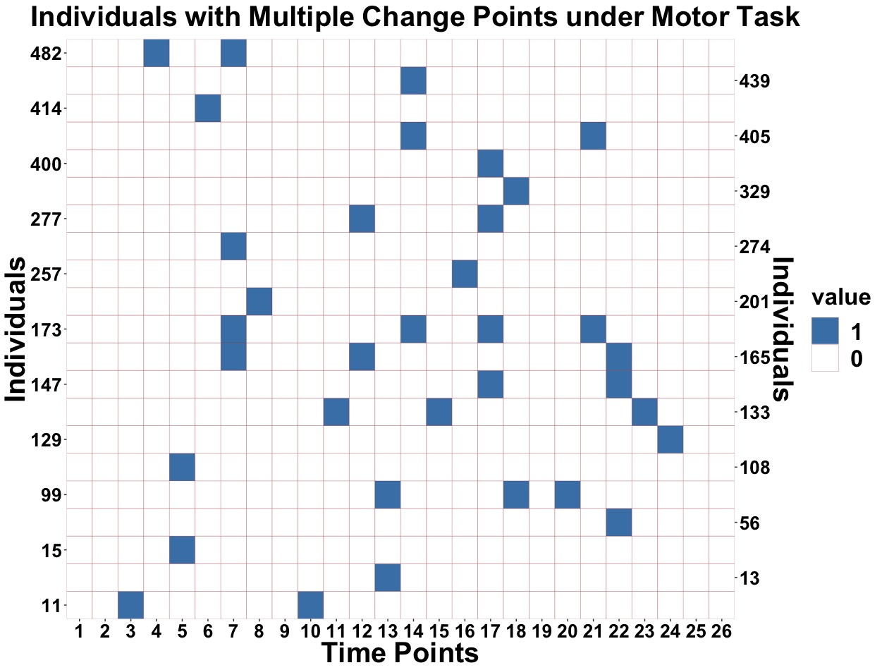
the motor task where we considered individuals with at least two change points. W detected individuals with multiple change points under motor task which is shown in Figure 19. There is no individual under motor task with more than four change points.
5.3 ADNI Dataset
We applied the hierarchical change point model on the previously described ADNI dataset, where the subjects are believed to be at a resting state. As anticipated, our model did not detect any change points in the dataset for both supernormals and health control groups. To test for model adequacy, we used the Watanabe-Akaike information criterion (WAIC) (Gelman et al., 2014). WAIC is a fully Bayesian approach to measure model accuracy computed with log pointwise posterior predictive density and then adding a correction for the effective number of parameters to adjust for overfitting. Table 4 provides the WAIC values for ADNI dataset with respect to the independence model (1), hierarchical covariance model (5) and the change point model (8) respectively. The WAIC values are lowest in the case of hierarchical covariance model which reaffirms the lacks of change points in resting state fMRI dataset. Higher WAIC values for the hierarchical change-point model suggests overfitting from a more complex model where the data do not have a changepoint.
6 Model Validation
In the following, we first consider an adhoc graphical summary measure of the posterior to justify the extension to hierarchical covariance model from the independence model for the HCP dataset. The exploratory analyses in Figures and were conducted to attest to two aspects of our hierarchical covariance model, namely i) using subject specific and variance components, and ii) using a common semi-orthogonal matrix across different subjects. A formal model comparison is done later using the WAIC (Gelman et al., 2014) to provide more support to our visual illustration in Figures and .
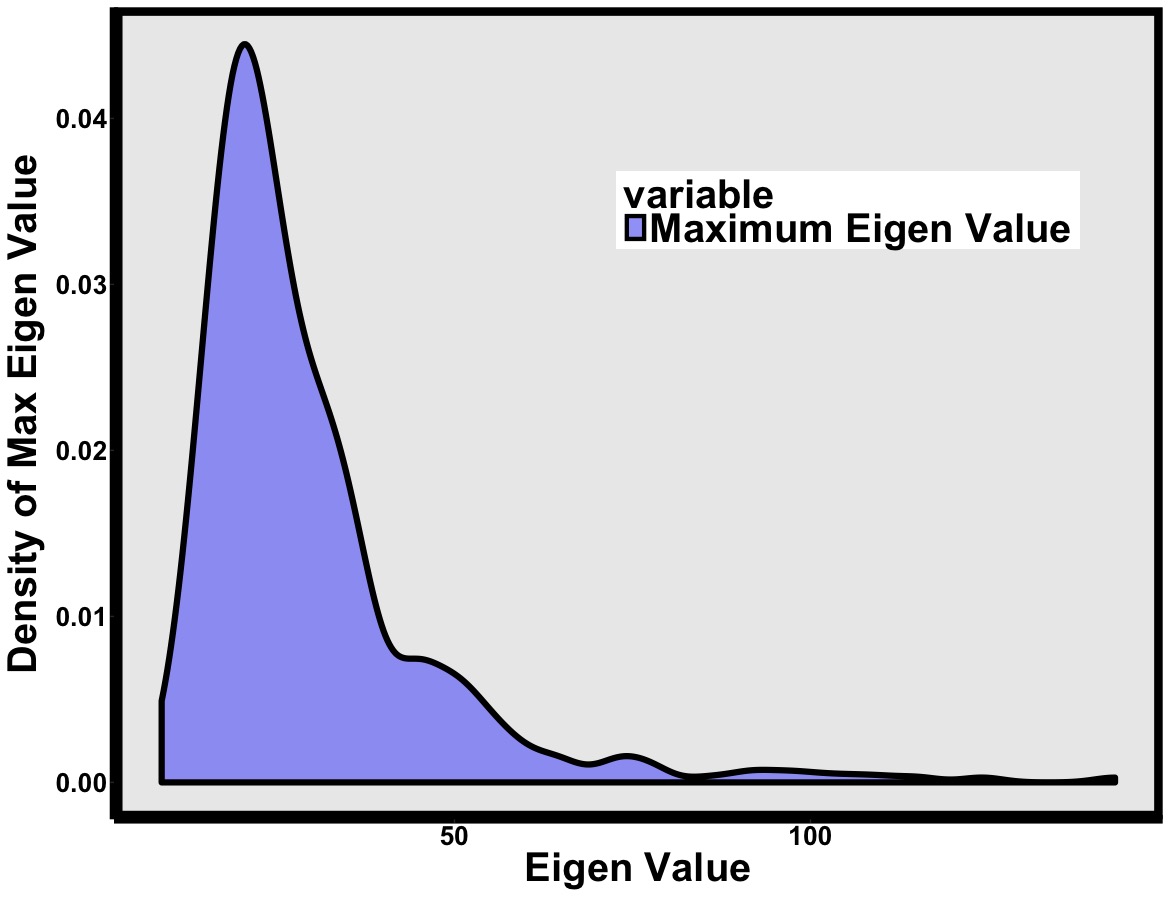
Figure shows the variation of the posterior estimate of the maximum eigenvalue and across the individuals, where data for each individual is fitted using the independence model on the time points. The density plot is obtained by smoothing posterior estimates across the individuals. As clearly seen, there is a substantial variability in both the variance component and the maximum eigenvalue which prompted us to consider individual specific and eigenvalues for the hierarchical covariance model.
Another important modeling assumption in (5) that requires empirical justification is the use of common semi-orthogonal matrix across all the individuals as opposed to having individual specific semi-orthogonal matrices in the independence model. In the following, we develop a simple diagnostic to this effect.

First we fit the independence model separately for each individual and for each we calculate the Karcher mean (Marks, 2012) of posterior samples of to obtain individual specific posterior estimate of the semi-orthogonal matrices, denoted . For each , variability of the estimate of the semi-orthogonal matrix is measured as where Karcher mean of and where . In Figure 21, “Different V” shows the histogram of describing the variability for the individual specific semi-orthogonal matrices. We generated data from (1) with individual specific set as for all individuals where and are the individual specific posterior estimates from the independence model. We then refit the independence model to this new dataset and acquired individual specific posterior estimates of the semi-orthogonal matrices = . Variability of these semi-orthogonal matrices is measured as for each . “Same V” in Figure 21 denotes the histogram of . Figure 21 clearly indicates a reduction in the variability of semi-orthogonal matrices if only a single semi-orthogonal matrix is considered across all individuals.

After fitting a complex Bayesian model, it is important to compare its predictive accuracy with other models, both simple and complex (Geisser and Eddy, 1979; Hoeting et al., 1999; Vehtari and Ojanen, 2012). Cross-validation and information criteria are two approaches to estimate out-of-sample predictive accuracy using within-sample fits. The deviance information criterion (DIC) (Spiegelhalter et al., 2002) is a generalization of the Akaike information criterion (AIC) (Akaike, 1998) for hierarchical settings. DIC has gained in popularity in recent years, in part through its implementation in the graphical modeling package BUGS, but it is known to suffer from issues from not being fully Bayesian. The Watanabe-Akaike information criterion (WAIC) (Watanabe, 2010) can be viewed as an improvement on the deviance information criterion (DIC) for Bayesian models. In this article, we use WAIC to compare the Independence model, the hierarchical covariance model and the its extension to detect changepoints. Computation time for the WAIC is negligible compared to the cost of fitting the model and obtaining posterior draws.
| Model | WAIC |
|---|---|
| Independence Model | |
| Hierarchical Covariance Model | |
| Hierarchical Change-point Model |
The WAIC values suggest progressively better fits as we move from the independence model to the most complex change point model.
7 Discussion
To discover patterns within the connectivity matrix of human brain as subjects perform specific tasks, we start with a simple Wishart distribution with an approximate low rank structure on the mean for modeling the covariance valued data. The methodology allows straightforward extension to a hierarchical model of multiple subjects where covariance valued time series is available for each subject. Another important extension is to develop a method for detecting a single change point in the covariance time series. Applying the methodology to the HCP data for the motor task reveals that the change point is associated with a particular regime switch of the experimental design. Also, the application to the resting state individuals in the ADNI study does not reveal any change point, which is in accordance with the expert opinions.
Another interesting application related to the HCP dataset is where the subjects are performing psychometric tasks and the goal is to understand how the connectivity evolves over time and whether a particular pattern in the time series motif is associated with the subjects “intelligence” or mental ability. In this case, the goal is to understand how the connectivity changes with time and it is important to allow more complex time varying structure in the evolution of the covariance matrix. Such applications also call for development of joint model of the mental ability scores and the connectivity matrices and is an interesting topic for future research.
For simplicity, we focused on a single Wishart distribution as a model for the covariance value data. A more flexible alternative beyond the Wishart family is to consider a mixture of Wishart distributions, particularly to allow for departures that are not captured by a single scale parameter. However, this comes with an additional burden of identifying and interpreting the component specific mean parameters that are required to be properly regularized to get a meaningful inference.
References
- Akaike, (1998) Akaike, H. (1998). Information theory and an extension of the maximum likelihood principle. In Selected papers of Hirotugu Akaike, pages 199–213. Springer.
- Barnard et al., (2000) Barnard, J., McCulloch, R., and Meng, X.-L. (2000). Modeling covariance matrices in terms of standard deviations and correlations, with application to shrinkage. Statistica Sinica, pages 1281–1311.
- Barry and Hartigan, (1993) Barry, D. and Hartigan, J. A. (1993). A Bayesian analysis for change point problems. Journal of the American Statistical Association, 88(421):309–319.
- Bhattacharya and Dunson, (2012) Bhattacharya, A. and Dunson, D. B. (2012). Simplex factor models for multivariate unordered categorical data. Journal of the American Statistical Association, 107(497):362–377.
- Bhattacharya et al., (2015) Bhattacharya, A., Pati, D., Pillai, N. S., and Dunson, D. B. (2015). Dirichlet–Laplace priors for optimal shrinkage. Journal of the American Statistical Association, 110(512):1479–1490.
- Boik, (2002) Boik, R. J. (2002). Spectral models for covariance matrices. Biometrika, 89(1):159–182.
- Buckner et al., (2011) Buckner, R., Krienen, F., Castellanos, A., Diaz, J., and Yeo, B. T. (2011). The organization of the human cerebellum estimated by intrinsic functional connectivity. American Journal of Physiology-Heart and Circulatory Physiology, 106:1125–1165.
- Carvalho et al., (2010) Carvalho, C. M., Polson, N. G., and Scott, J. G. (2010). The horseshoe estimator for sparse signals. Biometrika, 97(2):465–480.
- Cribben et al., (2013) Cribben, I., Wager, T., and Lindquist, M. (2013). Detecting functional connectivity change points for single-subject fmri data. Frontiers in computational neuroscience, 7:143.
- Dai et al., (2017) Dai, M., Zhang, Z., and Srivastava, A. (2017). Discovering change-point patterns in dynamic functional brain connectivity of a population. In International Conference on Information Processing in Medical Imaging, pages 361–372. Springer.
- Daniels, (2006) Daniels, M. J. (2006). Bayesian modeling of several covariance matrices and some results on propriety of the posterior for linear regression with correlated and/or heterogeneous errors. Journal of Multivariate Analysis, 97(5):1185–1207.
- Daniels and Kass, (1999) Daniels, M. J. and Kass, R. E. (1999). Nonconjugate Bayesian estimation of covariance matrices and its use in hierarchical models. Journal of the American Statistical Association, 94(448):1254–1263.
- Das and Daniels, (2014) Das, K. and Daniels, M. J. (2014). A semiparametric approach to simultaneous covariance estimation for bivariate sparse longitudinal data. Biometrics, 70(1):33–43.
- Delgado et al., (2000) Delgado, M., Nystrom, L., Fissell, C., Noll, D., and Fiez, J. (2000). Tracking the hemodynamic responses to reward and punishment in the striatum. Journal of Neurophysiology, 84:3072–3077.
- Destrieux et al., (2010) Destrieux, C., Fischl, B., Dale, A., and Halgren, E. (2010). Automatic parcellation of human cortical gyri and sulci using standard anatomical nomenclature. Neuroimage, 53(1):1–15.
- Finn et al., (2015) Finn, E. S., Shen, X., Scheinost, D., Rosenberg, M. D., Huang, J., Chun, M. M., Papademetris, X., and Constable, R. T. (2015). Functional connectome fingerprinting: identifying individuals using patterns of brain connectivity. Nature Neuroscience, 18(11):1664–1671.
- Flury, (1987) Flury, B. K. (1987). A hierarchy of relationships between covariance matrices. In Advances in multivariate statistical analysis, pages 31–43. Springer.
- Flury, (1984) Flury, B. N. (1984). Common principal components in k groups. Journal of the American Statistical Association, 79(388):892–898.
- Franks and Hoff, (2019) Franks, A. M. and Hoff, P. (2019). Shared subspace models for multi-group covariance estimation. Journal of Machine Learning Research, 20(171):1–37.
- Friston, (2011) Friston, K. J. (2011). Functional and effective connectivity: a review. Brain connectivity, 1(1):13–36.
- Gaskins and Daniels, (2016) Gaskins, J. and Daniels, M. (2016). Covariance partition priors: A Bayesian approach to simultaneous covariance estimation for longitudinal data. Journal of Computational and Graphical Statistics, 25(1):167–186.
- Gaskins et al., (2014) Gaskins, J., Daniels, M., and Marcus, B. (2014). Sparsity inducing prior distributions for correlation matrices of longitudinal data. Journal of Computational and Graphical Statistics, 23(4):966–984.
- Gaskins and Daniels, (2013) Gaskins, J. T. and Daniels, M. J. (2013). A nonparametric prior for simultaneous covariance estimation. Biometrika, 100(1):125–138.
- Geisser and Eddy, (1979) Geisser, S. and Eddy, W. F. (1979). A predictive approach to model selection. Journal of the American Statistical Association, 74(365):153–160.
- Gelman et al., (2014) Gelman, A., Hwang, J., and Vehtari, A. (2014). Understanding predictive information criteria for Bayesian models. Statistics and computing, 24(6):997–1016.
- (26) Glasser, M. F., Coalson, T. S., Robinson, E. C., Hacker, C. D., Harwell, J., Yacoub, E., Ugurbil, K., Andersson, J., Beckmann, C. F., Jenkinson, M., et al. (2016a). A multi-modal parcellation of human cerebral cortex. Nature, 536(7615):171–178.
- (27) Glasser, M. F., Smith, S. M., Marcus, D. S., Andersson, J. L., Auerbach, E. J., Behrens, T. E., Coalson, T. S., Harms, M. P., Jenkinson, M., Moeller, S., et al. (2016b). The human connectome project’s neuroimaging approach. Nature Neuroscience, 19(9):1175–1187.
- Glasser et al., (2013) Glasser, M. F., Sotiropoulos, S. N., Wilson, J. A., Coalson, T. S., Fischl, B., Andersson, J. L., Xu, J., Jbabdi, S., Webster, M., Polimeni, J. R., et al. (2013). The minimal preprocessing pipelines for the human connectome project. Neuroimage, 80:105–124.
- Glover, (2011) Glover, G. H. (2011). Overview of functional magnetic resonance imaging. Neurosurgery Clinics, 22(2):133–139.
- Golosnoy et al., (2012) Golosnoy, V., Gribisch, B., and Liesenfeld, R. (2012). The conditional autoregressive Wishart model for multivariate stock market volatility. Journal of Econometrics, 167(1):211–223.
- Gouriéroux et al., (2009) Gouriéroux, C., Jasiak, J., and Sufana, R. (2009). The Wishart autoregressive process of multivariate stochastic volatility. Journal of Econometrics, 150(2):167–181.
- Hindriks et al., (2016) Hindriks, R., Adhikari, M., Murayama, Y., Ganzetti, M., Mantini, D., Logothetis, N., and Deco, G. (2016). Can sliding-window correlations reveal dynamic functional connectivity in resting-state fmri? NeuroImage, 127:242 – 256.
- Hoeting et al., (1999) Hoeting, J. A., Madigan, D., Raftery, A. E., and Volinsky, C. T. (1999). Bayesian model averaging: a tutorial. Statistical science, pages 382–401.
- Hoff, (2013) Hoff, P. (2013). Bayesian analysis of matrix data with rstiefel. R-vignette.
- (35) Hoff, P. D. (2009a). A hierarchical eigenmodel for pooled covariance estimation. Journal of the Royal Statistical Society: Series B (Statistical Methodology), 71(5):971–992.
- (36) Hoff, P. D. (2009b). Simulation of the matrix Bingham–von Mises–Fisher distribution, with applications to multivariate and relational data. Journal of Computational and Graphical Statistics, 18(2):438–456.
- Hutchison et al., (2013) Hutchison, R. M., Womelsdorf, T., Allen, E. A., Bandettini, P. A., Calhoun, V. D., Corbetta, M., Della Penna, S., Duyn, J. H., Glover, G. H., Gonzalez-Castillo, J., et al. (2013). Dynamic functional connectivity: promise, issues, and interpretations. Neuroimage, 80:360–378.
- Ian L. Dryden and Zhou, (2009) Ian L. Dryden, A. K. and Zhou, D. (2009). Non-euclidean statistics for covariance matrices, with applications to diffusion tensor imaging. The Annals of Applied Statistics, 3(3):1102–1123.
- Jbabdi et al., (2015) Jbabdi, S., Sotiropoulos, S. N., Haber, S. N., Van Essen, D. C., and Behrens, T. E. (2015). Measuring macroscopic brain connections in vivo. Nature Neuroscience, 18(11):1546.
- Khatri and Mardia, (1977) Khatri, C. and Mardia, K. V. (1977). The von Mises–Fisher matrix distribution in orientation statistics. Journal of the Royal Statistical Society: Series B (Methodological), 39(1):95–106.
- Leonard et al., (1992) Leonard, T., Hsu, J. S., et al. (1992). Bayesian inference for a covariance matrix. The Annals of Statistics, 20(4):1669–1696.
- Li and Pati, (2017) Li, H. and Pati, D. (2017). Variable selection using shrinkage priors. Computational Statistics & Data Analysis, 107:107–119.
- (43) Lin, F., Ren, P., Mapstone, M., Meyers, S. P., Porsteinsson, A., Baran, T. M., Initiative, A. D. N., et al. (2017a). The cingulate cortex of older adults with excellent memory capacity. Cortex, 86:83–92.
- (44) Lin, F. V., Wang, X., Wu, R., Rebok, G. W., and Chapman, B. P. (2017b). Identification of successful cognitive aging in the alzheimer’s disease neuroimaging initiative study. Journal of Alzheimer’s Disease, 59(1):101–111.
- Lindquist et al., (2014) Lindquist, M. A., Xu, Y., Nebel, M. B., and Caffo, B. S. (2014). Evaluating dynamic bivariate correlations in resting-state fmri: a comparison study and a new approach. NeuroImage, 101:531–546.
- Lopes and West, (2004) Lopes, H. and West, M. (2004). Bayesian model assessment in factor analysis. Statistica Sinica, 14:41–67.
- Marks, (2012) Marks, J. (2012). Mean variants on matrix manifolds. Doctor of Philosophy (Ph.D.) Thesis, Colorado State University.
- Miller et al., (2016) Miller, K. L., Alfaro-Almagro, F., Bangerter, N. K., Thomas, D. L., Yacoub, E., Xu, J., Bartsch, A. J., Jbabdi, S., Sotiropoulos, S. N., Andersson, J. L., et al. (2016). Multimodal population brain imaging in the uk biobank prospective epidemiological study. Nature neuroscience, 19(11):1523.
- Monti et al., (2014) Monti, R., Hellyer, P., Sharp, D., Leech, R., Anagnostopoulos, C., and Montana, G. (2014). Estimating time-varying brain connectivity networks from functional mri time series. NeuroImage, 103:427 – 443.
- Park and Friston, (2013) Park, H.-J. and Friston, K. (2013). Structural and functional brain networks: from connections to cognition. Science, 342(6158):1238411.
- Pati et al., (2014) Pati, D., Bhattacharya, A., Pillai, N. S., and Dunson, D. (2014). Posterior contraction in sparse Bayesian factor models for massive covariance matrices. The Annals of Statistics, 42(3):1102–1130.
- Polson and Scott, (2012) Polson, N. G. and Scott, J. G. (2012). On the Half-Cauchy Prior for a Global Scale Parameter. Bayesian Analysis, 7(4):887–902.
- Pourahmadi, (2011) Pourahmadi, M. (2011). Covariance estimation: The glm and regularization perspectives. Statistical Science, 26(3):369–387.
- Pourahmadi et al., (2007) Pourahmadi, M., Daniels, M. J., and Park, T. (2007). Simultaneous modelling of the cholesky decomposition of several covariance matrices. Journal of Multivariate Analysis, 98(3):568–587.
- Schott, (1999) Schott, J. R. (1999). A test for proportional covariance matrices. Computational statistics & data analysis, 32(2):135–146.
- Schott, (2001) Schott, J. R. (2001). Some tests for the equality of covariance matrices. Journal of statistical planning and inference, 94(1):25–36.
- Smith et al., (2015) Smith, S. M., Nichols, T. E., Vidaurre, D., Winkler, A. M., Behrens, T. E., Glasser, M. F., Ugurbil, K., Barch, D. M., Van Essen, D. C., and Miller, K. L. (2015). A positive-negative mode of population covariation links brain connectivity, demographics and behavior. Nature Neuroscience, 18(11):1565–1567.
- Spiegelhalter et al., (2002) Spiegelhalter, D. J., Best, N. G., Carlin, B. P., and Van Der Linde, A. (2002). Bayesian measures of model complexity and fit. Journal of the royal statistical society: Series B (statistical methodology), 64(4):583–639.
- Stingo et al., (2013) Stingo, F. C., Guindani, M., Vannucci, M., and Calhoun, V. D. (2013). An integrative bayesian modeling approach to imaging genetics. Journal of the American Statistical Association, 108(503):876–891.
- Turner, (2016) Turner, R. (2016). Uses, misuses, new uses and fundamental limitations of magnetic resonance imaging in cognitive science. Philosophical Transactions of the Royal Society B: Biological Sciences, 371(1705):20150349.
- Tzourio-Mazoyer et al., (2002) Tzourio-Mazoyer, N., Landeau, B., Papathanassiou, D., Crivello, F., Etard, O., Delcroix, N., Mazoyer, B., and Joliot, M. (2002). Automated anatomical labeling of activations in spm using a macroscopic anatomical parcellation of the mni mri single-subject brain. Neuroimage, 15(1):273–289.
- van der Pas et al., (2014) van der Pas, S. L., Kleijn, B. J. K., and van der Vaart, A. W. (2014). The horseshoe estimator: Posterior concentration around nearly black vectors. Electronic Journal of Statistics, 8:2585–2618.
- Van Essen et al., (2013) Van Essen, D. C., Smith, S. M., Barch, D. M., Behrens, T. E., Yacoub, E., Ugurbil, K., Consortium, W.-M. H., et al. (2013). The wu-minn human connectome project: an overview. Neuroimage, 80:62–79.
- Vehtari and Ojanen, (2012) Vehtari, A. and Ojanen, J. (2012). A survey of Bayesian predictive methods for model assessment, selection and comparison. Statistics Surveys, 6:142–228.
- Vershynin, (2012) Vershynin, R. (2012). Introduction to the non-asymptotic analysis of random matrices. Compressed Sensing, Theory and Applications. Edited by Y. Eldar and G. Kutyniok. Cambridge University Press, pages 210–268.
- Warnick et al., (2018) Warnick, R., Guindani, M., Erhardt, E., Allen, E., Calhoun, V., and Vannucci, M. (2018). A bayesian approach for estimating dynamic functional network connectivity in fmri data. Journal of the American Statistical Association, 113(521):134–151.
- Watanabe, (2010) Watanabe, S. (2010). Asymptotic equivalence of Bayes cross validation and widely applicable information criterion in singular learning theory. Journal of Machine Learning Research, 11(Dec):3571–3594.
- Weiner et al., (2010) Weiner, M. W., Aisen, P. S., Jack Jr, C. R., Jagust, W. J., Trojanowski, J. Q., Shaw, L., Saykin, A. J., Morris, J. C., Cairns, N., Beckett, L. A., et al. (2010). The Alzheimer’s disease neuroimaging initiative: progress report and future plans. Alzheimer’s & Dementia, 6(3):202–211.
- Yu et al., (2017) Yu, P. L., Li, W., and Ng, F. (2017). The generalized conditional autoregressive Wishart model for multivariate realized volatility. Journal of Business & Economic Statistics, 35(4):513–527.
- Zhang et al., (2018) Zhang, Z., Allen, G., Zhu, H., and Dunson, D. (2018). Relationships between human brain structural connectomes and traits. bioRxiv, page 256933.
Appendix
In Appendix A, we explore a dynamic extension of our hierarchical change point model (8). Appendix B contains sensitivity analysis for the hierarchical change point model (8) and some additional simulations to study robustness. Appendix C contains results for the gambling task for the HCP data. In Appendix D, we validate our assumption of considering . Appendix E & F contain details of posterior computation under the independence & hierarchical models respectively.
Appendix A Dynamic Change Point Model
In our current change-point estimation framework, the observational units before and after the change-point are assumed to be independent and identically distributed. A dynamic extension of our model is certainty interesting to incorporate the dependence across the time-points. To that end, we explore an auto-regressive Wishart process on the subject specific loadings. This is studied under the hierarchical change point model for one subject with a single change point:
| (11) |
We use the same orthogonal factor model type decomposition on at each time point of an individual. As a parsimonious model for the time dependent covariance matrices, the orthogonal matrix is held constant with subject specific time varying process for the loadings and subject specific variance components. For computational convenience, we consider which are assumed to evolve following an auto-regressive process:
The diagonal elements at the first time point are shrunk using global and local shrinkage:
| (13) | ||||
Here , are the global shrinkage parameters while the , parameters allow for coordinate specific deviations. We place independent half-Cauchy priors on the local parameters and half-Cauchy prior truncated to on the global parameters. Also, and with .
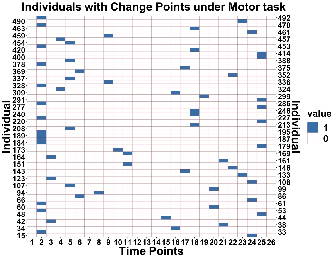
We detected change points of individuals from the dynamic change point model which is provided in Figure A.1. There are indeed certain change points which are detected by both (8) and (11). For example, the change points for individual , and are detected at th, rd and th time point using both the models. Although the specific dynamic framework can be extended to a full-blown dynamic model, initial indications of the WAIC values suggest that it may not be a good fit for the current dataset. We leave this as a topic for future research.
Appendix B Sensitivity and robustness analysis of the hierarchical change point model
We considered different values of the fitted rank and ran the hierarchical change point model (8) on the HCP dataset under the Motor task to check the sensitivity of the results with respect to the fitted rank. The findings are provided in Table A1. We obtained similar results for 26 individuals from different values of fitted ranks which are provided in the last column of Table A1. Next we considered five different initializations for the model parameters in (8) and fixed . Detected change points with the corresponding individuals are shown in Table A2 and the frequently appeared individuals for all those 5 settings are provided in last column of the table. The description of these initial values are provided next. For setting , we set to be , and . In case of setting , we consider to be , and values for all values of were same with setting . Values of was set to be , and same value for all parameters for setting . In setting , we have to be , and . In case of setting , we consider to be , and .
We conducted another experiment to test the robustness of the change point model when the data generating distribution indeed has correlation across time points. We simulated data from the time varying change point model (11) consisting of subjects with time points. All the subjects have individual specific change points which are generated uniformly in the interval . For clarity, any parameter with subscript “1” correspond to the pre-change-point regime (Group 1) and the ones with subscript “2” corresponds to the post-change-point (Group 2). Individual specific variances and are generated from . Local parameters and global parameters are generated from half-Cauchy distribution. and are generated by following equation (13). We use AR(1) process (A) to generate rest of the columns of and . Figure B.1 shows that our non-time varying model model is able to detect the individual specific change points for 60% cases even though the data is generated from the time varying hierarchical change point model.


| Common Ind | |||||||||
|---|---|---|---|---|---|---|---|---|---|
| Change Point | Ind | Change Points | Ind | Change Points | Ind | Change Points | Ind | Change Points | Ind |
| Setting 1 | Setting 2 | Setting 3 | Setting 4 | Setting 5 | Common Ind | ||||||
|---|---|---|---|---|---|---|---|---|---|---|---|
| Change Point | Ind | Change Points | Ind | Change Points | Ind | Change Points | Ind | Change Points | Ind | Change Points | Ind |

Appendix C Case study for gambling task of HCP dataset
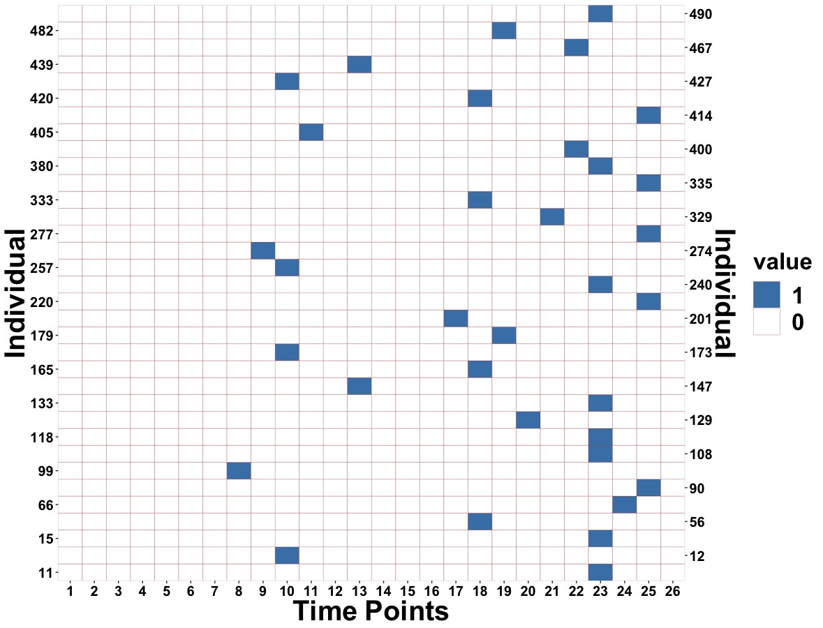
A detailed description of the gambling task corresponding to HCP is in Delgado et al., 2000. We applied our hierarchical change point model on data which was scaled with subject specific minimum eigen value. We are able to detect individuals with change points under Gambling task. In Figure C.1 we labeled the individuals with their corresponding change points. Figure 1(a) consists of 70 individuals with their most prominent change point detected through the hierarchical model. Figure 1(b) shows the overall pattern of the most prominent change points across all the individuals. The histogram in Figure 1(b) shows that more than 10% individuals have change points at .


Next we extended our study to detect multiple change points under gambling task. We applied the methodology discussed in section 5.2 on individuals under gambling task and detected multiple change points for different individuals. In Figure C.2, we listed the individuals with at least two change points and their corresponding change points.

Appendix D Validation of the value of
In this section, we validate the choice of based on WAIC. Under the same simulation setting as in Section 3.1.1, the data is generated from the independence model (1) by setting the true values of in . The fitted values of are varied over a range and corresponding WAIC values are reported in Table (A3). Irrespective of the true value of , the lowest WAIC value is obtained when . For the HCP data analysis, we compare the WAIC values from the hierarchical change point model (8) for several values of as shown in Table (A4). The lowest WAIC is attained at .
| True | True | True | |||||||||
|---|---|---|---|---|---|---|---|---|---|---|---|
| WAIC | WAIC | WAIC | WAIC | WAIC | WAIC | ||||||
| 11 | 223980.5 | 16 | 982594.9 | 11 | 224046.5 | 16 | 891307.5 | 11 | 227826.6 | 16 | 832607.7 |
| 12 | 350710.9 | 17 | 1161531.7 | 12 | 331893.7 | 17 | 1052557.1 | 12 | 326247.8 | 17 | 980285.6 |
| 13 | 492837.7 | 18 | 1346223.5 | 13 | 454632.8 | 18 | 1219633.2 | 13 | 437647.2 | 18 | 1133538.3 |
| 14 | 646175.0 | 19 | 1535622.7 | 14 | 590192.5 | 19 | 1391076.2 | 14 | 559376.4 | 19 | 1291091.1 |
| 15 | 810530.4 | 20 | 1729035.9 | 15 | 736743.1 | 20 | 1566453.2 | 15 | 692127.0 | 20 | 1452505.0 |
| Real Data Analysis | |||
|---|---|---|---|
| WAIC | WAIC | ||
| 11 | 196739 | 16 | 257329 |
| 12 | 209801 | 17 | 271796 |
| 13 | 218313 | 18 | 289761 |
| 14 | 233022 | 19 | 297537 |
| 15 | 242873 | 20 | 312590 |
Appendix E Posterior Computation under Independence Model
We first record two useful identities. We have
,
where . Moreover,
,
where .
- •
Likelihood under Independence Model: The joint likelihood of is
,
where .With the transformation , the joint likelihood of is
We now describe the full-conditional distributions that are used to implement a Metropolis within Gibbs sampler to sample from the joint posterior of . We use the notation to denote the full conditional distribution of a parameter.
- •
Full conditional of V:
We have,
.
This is a Bingham distribution, which can be sampled using the package Rstiefel in R. - •
Full conditional of :
We decomposed and considered and a transformation for . The full-conditional of is give by
,
To sample from the above, we consider a slice-sampling scheme. Specifically, augment a latent variable such that the joint distribution of is
.
It is clearly seen that the marginal distribution of is preserved under this joint distribution. We then successively sample from the conditionals and . We have
Uniform ,
Gamma(shape, rate ). - •
Full conditional of :
The full conditional of is
.
where . We use a Metropolis–Hastings step to sample using a normal random-walk proposal as with standard deviation . We accept with probability where - •
Full conditional of :
,
where . This implies
Inverse-Gamma.
Appendix F Posterior Computation and Algorithm under Hierarchical Model
The joint likelihood of under the hierarchical covariance model (5) is
With the transformation , the joint likelihood of is
Now we only describe detailed steps to derive the full-conditional of V. For the rest of the parameters, we cycled through the subject specific full-conditionals which are similarly derived following the posterior computation steps under the Independence model (1). We have
where and . The detailed steps of the identity used in (6) are given as
The full-conditional of under the hierarchical covariance model (5) can thus be expressed as
To sample from the above, we follow the steps in §3.3 of Hoff, 2009b and write with . Here, is an orthonormal basis for the null space of and is expressed as because . The conditional density of is derived as in Hoff, 2009b as
We iterate through the steps 1–4 for each to obtain samples from the density (6):
1) = null space of and .
2) .
3) Sample from a vector Bingham() density using the package rsteifel (Hoff, 2013).
4) Set .