Design Verifiably Correct Model Patterns to Facilitate Modeling Medical Best Practice Guidelines with Statecharts
(Technical Report)

Chunhui Guo¹, Zhicheng Fu¹, Zhenyu Zhang², Shangping Ren^2,1, Lui Sha³ Affiliation: ¹Department of Computer Science, Illinois Institute of Technology, Chicago, IL 60616, USA
²Department of Computer Science, San Diego State University, San Diego, CA 92182, USA
³Department of Computer Science, University of Illinois at Urbana-Champaign, Urbana, IL 61801, USA
{cguo13, zfu11}@hawk.iit.edu, {zzhang4430, sren}@sdsu.edu, lrs@illinois.edu

Abstract

Improving patient care safety is an ultimate objective for medical cyber-physical systems. A recent study shows that the patients’ death rate can be significantly reduced by computerizing medical best practice guidelines. To facilitate the development of computerized medical best practice guidelines, statecharts are often used as a modeling tool because of their high resemblances to disease and treatment models and their capabilities to provide rapid prototyping and simulation for clinical validations. However, some implementations of statecharts, such as Yakindu statecharts, are priority-based and have synchronous execution semantics which makes it difficult to model certain functionalities that are essential in modeling medical guidelines, such as two-way communications and configurable execution orders. Rather than introducing new statechart elements or changing the statechart implementation’s underline semantics, we use existing basic statechart elements to design model patterns for the commonly occurring issues. In particular, we show the design of model patterns for two-way communications and configurable execution orders and formally prove the correctness of these model patterns. We further use a simplified airway laser surgery scenario as a case study to demonstrate how the developed model patterns address the two-way communication and configurable execution order issues and their impact on validation and verification of medical safety properties.

Index Terms:

Verifiably correct model patterns, medical guideline modeling, Statechart models.

I Introduction and Related Work

A study shows that the patients’ death rate can be significantly reduced by computerizing medical best practice guidelines [1]. Developing computerized disease and treatment models from medical best practice handbooks needs close interactions with medical professionals. In addition, to satisfy the safety and correctness requirements, the derived models also need to be clinically validated and formally verified. Over past two decades, many computer executable medical best practice guideline models are developed, such as Asbru [2], GLIF [3], GLARE [4], EON [5], and PROforma [6]. Rahmaniheris et al. [7] have developed an organ-centric approach to model medical best practice guidelines with statecharts, which enable rapid prototyping and allow quick clinical validations by medical staff through simulations. Tan et al. [8] proposed a design pattern for wireless medical Cyber-Physical Systems (CPS). Jiang et al. [9] presented a timed automata and synchronous dataflow based framework for system design. Guo et al. [10, 11] proposed approaches to model and integrate medical resource availability and relationships in existing medical guideline models. To help improve clinical validation, Wu et al. have developed a workflow adaptation protocol [12] to help physicians safely adapt workflows to react to patient adverse events and a treatment validation protocol [13] to enforce the correct execution sequence of performing a treatment based on preconditions validation, side effects monitoring, and expected responses checking. Both the workflow adaptation and treatment validation protocol are based on pathophysiological models. In addition, based on organ-specific physiology, a system that integrates medical devices into semi-autonomous clusters in a network-fail-safe manner has also been developed by Kang et al. [14]. Christov et al. [15] proposed an approach to detect whether the performed medical procedures have deviated from the recommended ways to perform the medical procedures, i.e., medical best practices. To formally verify safety properties of medical guideline models, Guo et al. [16] presented an approach to transform statecharts to timed automata. Runtime verification techniques [17, 18] were also applied to improve safety of medical guideline systems at code level.

Most existing medical best practice guidelines in hospital handbooks are represented by flowcharts [19] which are very similar to statecharts [20], so are many medical disease models and treatment models. In addition to the high similarities between medical models and statecharts, statecharts are executable and have become a widely used model in designing complex systems, such as avionics [21], air traffic control systems [22], and medical systems [7, 23, 16]. These distinguishing features of statecharts have inspired us to use it as a computerized representation for medical best practice guidelines. However, there are functionalities that are essential in medical operations, such as two-way communications and configurable execution orders, which are not directly supported by some open source statechart modeling tools, such as Yakindu. We use the following two examples to illustrate the need of two-way communications and configurable execution orders in medical domain. By two-way communications we mean two statecharts can communicate with each other, and by configurable execution orders we mean the execution orders can be configured by users without change the model itself.

Example 1.

Laser surgery [24] is a surgical procedure that uses a laser to remove problematic tissues and is widely used in airway surgery, thoracic surgery, eye surgery, etc. For airway laser surgery, there are two potential dangers: (1) an accidental burn if both laser and ventilator are activated; and (2) a low-oxygen shock if the Saturation of Peripheral Oxygen ( $\mathtt{SpO}$ ) level of the patient decreases below a given threshold (assume $95\%$ ) [25]. To prevent the potential dangers, the airway laser and the ventilator must be able to communicate with each other bidirectionally, i.e., the communication needs to be two-way. In particular, when the surgery starts, the airway laser turns on and notifies the ventilator to turn off; and when the patient’s $\mathtt{SpO}$ level becomes below $95\%$ , the ventilator turns on and notifies the airway laser to turn off.

Example 2.

In the chronic cough treatment guideline [26], chest radiography has to be performed before sputum test and bronchoscopy, but the guideline does not specify the order between sputum test and bronchoscopy. The physicians can choose the medical procedure order $\mathtt{chest\ radiography}$ $\prec$ $\mathtt{sputum\ test}$ $\prec$ $\mathtt{bronchoscopy}$ or $\mathtt{chest\ radiography}$ $\prec$ $\mathtt{bronchoscopy}$ $\prec$ $\mathtt{sputum\ test}$ based on their experiences/preferences and medical resource availability.

Without the two-way communication support, the laser and the ventilator in the airway laser surgery can be both activated and cause surgery fire. We present more details about the scenario in the case study, i.e., Section V. Without the configurable execution order support, if a physician deviate from the medical procedure execution order specified in a medical guideline system, the system can not identify whether or not the deviation is safe. Hence, supporting two-way communications and configurable execution orders are very important for modeling medical best practice guidelines.

However, most existing medical guideline modeling languages, such as Asbru [2], GLIF [3], and PROforma [27], do not support these essential functionalities. Althouh Simulink Stateflow [28], a statechart variant from Matlab [29], supports two-way communications through condition actions and preemptive execution semantics, it does not support execution order change without modifying existing models.

Open source Yakindu statecharts are priority-based and have synchronous execution semantics. With such execution semantics, only higher priority statecharts can send events to lower priority statecharts, but not the other way around. In addition, each statechart is pre-assigned an unique priority to determine its execution order when a model is established.

A naive approach to implement two-way communication functionality is to use global variables shared among multiple statecharts. However, using global variables has known disadvantages of increased difficulty and complexity to maintain data consistence. An alternative is to take a similar approach as in Stateflow [28] by introducing new elements into Yakindu to interrupt the execution of the event sender statechart and resume after handling the event. However, such approach changes Yakindu statecharts’ underline execution semantics and violates Yakindu statecharts’ original design goal.

To address the configurable execution order issue, a straight forward approach is to customize medical guideline statechart models based on execution orders provided by physicians. However, the approach faces the following challenges: (1) a medical guideline model requires a variant for every physician to facilitate different execution orders, which is cumbersome for practical use; and (2) engineers need to be involved in clinical care to manually modify medical guideline models when physicians change execution orders.

The major challenge of implementing the essential functionalities in modeling medical guidelines, such as two-way communications and configurable execution orders, is that it has to be effortless for medical professionals to validate its correctness and formally verifiable at reasonable cost. The paper presents an approach to apply model patterns to support these essential functionalities. The model patterns do not introduce new statechart elements nor change statecharts’ underline execution semantics. Hence, the model patterns do not require additional effort for medical professionals to validate their correctness. In addition, our previous work [16] can also be applied to formally verify medical guideline models that apply the model patterns.

The rest of the paper is organized as follows. Section II briefly introduce the preliminary work on developing verifiably safe medical best practice guidelines with statecharts. We design the two-way communication model pattern and configurable execution order model pattern in Section III and formally prove the model patterns’ correctness in Section IV. A case study of a simplified airway laser surgery scenario is performed in Section V. We present some discussions in Section VI and conclude in Section VII.

II Preliminary Work

Our previous work [16] presents an approach to build verifiably safe executable medical guideline models in two steps: (1) use statecharts [20] to model medical guidelines and interact with medical professionals to validate the correctness of the medical guideline models; and (2) automatically transform medical guideline statecharts to timed automata [30] by the developed Y2U tool [16] to formally verify safety properties. In this section, we use the simplified airway laser surgery scenario in Example 1 as an example to briefly summarize the process of building verifiably safe executable medical guideline models.

II-A Model Medical Guidelines with Statecharts

We use Yakindu statecharts to model the simplified airway laser surgery, as shown in Fig. 1. Both laser and ventilator are modeled as a statechart with three states ( $\mathtt{On}$ , $\mathtt{Off}$ , and $\mathtt{Syn}$ ) to represent the devices’ operation status. To prevent the accidental burn danger caused by laser and ventilator are both activated, we add the $\mathtt{Syn}$ state to ensure that the laser/ventilator’s activation procedure is delayed one step after the ventilator/laser’s deactivation procedure. The initial state of the airway laser surgery system is: the laser is off and the ventilator is on to supply oxygen to the patient. When the ventilator is turned off, we assume that the patient’s $\mathtt{SpO}$ level decreases by 1 every second.

Refer to caption — Fig. 1: Simplified Airway Laser Surgery Statechart Model

In the statechart shown in Fig. 1, when an operating surgeon sends the $\mathtt{startLaser}$ event to the $\mathtt{laser}$ to operate the surgery, the $\mathtt{laser}$ sends the $\mathtt{deactivateVen}$ event to stop oxygen supply. If the patient’s $\mathtt{SpO}$ level reduces below $95\%$ , the $\mathtt{ventilator}$ turns on to supply oxygen and sends the $\mathtt{deactivateLaser}$ event to stop the $\mathtt{laser}$ .

II-B Verifiably Safe Statecharts

Statecharts contain basic elements, such as states and transitions, and advanced elements, such as composite states. Although these advanced elements provide modeling convenience, they increase the difficulty of both clinical validation and formal verification. As stated in the literature, one of the keys to achieving system safety at reasonable cost is a serious and sustained commitment to simplicity [31, 32]. To reduce the difficulty in both clinical validation and formal verification, our previous work [33] proposes a pattern-based statechart modeling approach to model medical guidelines with basic statechart elements and model patterns which are built upon these basic elements to implement advanced statechart elements.

To formally verify medical guideline statechart models, our previous work [16] presents an approach to transform statechart models to timed automata. There are three key differences between Yakindu statecharts and UPPAAL timed automata: (1) syntactic difference: Yakindu statecharts have some elements that are not directly supported by UPPAAL timed automata, such as event and timing trigger; (2) execution semantics difference: Yakindu model is deterministic and has synchronous execution semantics while the execution of UPPAAL model is non-deterministic and asynchronous; and (3) simultaneous events difference: Yakindu supports simultaneous events while UPPAAL does not.

Our transformation handles above three key differences by following approaches: (1) syntactic difference: define 5 transformation rules for basic Yakindu statecharts elements, i.e., state, transition, state action, event, and timing trigger; (2) execution semantics difference: design 2 transformation rules to implement transition trigger determinism and statechart execution determinism, and use the lockstep method [34] to force synchronous execution; and (3) simultaneous events difference: design an event stack to simulate simultaneous event mechanism in UPPAAL timed automata.

To ensure that the formal verification results in timed automata is consistent with the statecharts, we prove the transformation correctness. The approach also provides the capability to trace back paths that fail safety properties from timed automata to statecharts. Although our approach only transforms basic Yakindu statechart elements, it is sufficient to provide formal verification functionality for medical guideline statecharts because the advanced statechart elements can be represented by basic elements [33].

III Model Pattern Design

Some statecharts have priority-based, deterministic, and synchronous execution semantics, such as Yakindu statecharts. The execution semantics make it difficult to model certain features that are essential in modeling medical guidelines, such as two-way communications and configurable execution orders. In this section, we design model patterns to support two-way communications and configurable execution orders without changing statecharts’ underline execution semantics nor introducing new statechart elements.

III-A Design Model Pattern for Two-Way Communication

In statechart models with multiple statecharts, two-way communications are essential. For instance, the $\mathtt{laser}$ statechart and $\mathtt{ventilator}$ statechart in Fig. 1 require two-way communications. We represent the two-way communication requirement by the statechart model shown in Fig. 2. The two-way communication feature means that statechart $\mathtt{S1}$ can receive event $\mathtt{EB}$ raised by $\mathtt{S2}$ and statechart $\mathtt{S2}$ can receive event $\mathtt{EA}$ raised by $\mathtt{S1}$ . However, if statechart $\mathtt{S1}$ has higher priority than statechart $\mathtt{S2}$ , the event $\mathtt{EB}$ can not be passed from $\mathtt{S2}$ to $\mathtt{S1}$ due to priority-based and synchronous execution semantics.

In this section, we design a model pattern to support two-way communication in statecharts. The model pattern design needs to satisfy the following two criteria: (1) it does not changing statecharts’ underline execution semantics; and (2) it does not introduce new statechart elements. The reason of these two criteria is that new statechart elements and new execution semantic rules increase the difficulty for medical professionals to validate medical guideline models. Based on the model pattern design criteria, our strategy to support two-way communication is to queue all raised events, add logic execution cycles, and re-raise the queued events in the added logic cycles. Note that each added logic execution cycle takes one CPU time unit which is negligible compared to clock time. Under the two-way communication model pattern, the statechart $\mathtt{S2}$ in Fig. 2 can send event $\mathtt{EB}$ to statechart $\mathtt{S1}$ .

We take Yakindu statecharts as an example to implement the two-way communication model pattern. In particular, for each execution cycle (we call it normal cycle), we queue all raised events. After each normal execution cycle, we add $n-1$ logic cycles to re-raise queued events, where $n$ is the number of statecharts. In each logic cycle, each queued event is only visible to statecharts whose priorities are higher than the event raiser, as lower priority statecharts have already received the queued event in the normal cycle. Furthermore, at each logic cycle, only those transitions that are triggered by queued events are executed. This constraint is to ensure that the logic cycle does not change the model behavior other than facilitate higher priority statecharts to receive events from lower priority statecharts.

The two-way communication model pattern contains a $\mathtt{Manager}$ statechart and a interface $\mathtt{TWC}$ , as shown in Fig. 3. In particular, the $\mathtt{Manager}$ statechart has the highest priority in the model and initializes the event queues. The interface $\mathtt{TWC}$ declares four functions: $\mathtt{initEventQueue()}$ , $\mathtt{push()}$ , $\mathtt{pop()}$ , and $\mathtt{isNormalExe()}$ .

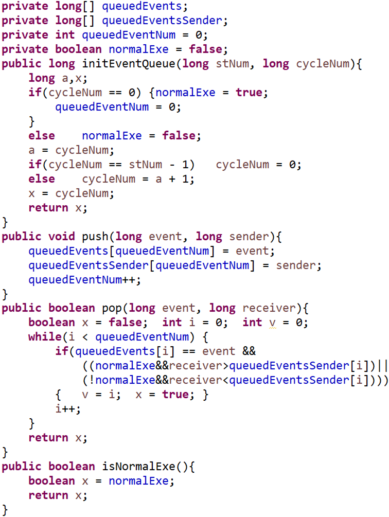
We define a Java class $\mathtt{TWC}$ shown in Fig. 4 to implement the $\mathtt{TWC}$ interface. The event queue is implemented by two arrays $\mathtt{queuedEvents}$ and $\mathtt{queuedEventsSender}$ to store raised events and their corresponding senders. The $\mathtt{TWC}$ class also includes a boolean variable $\mathtt{normalExe}$ that indicates if the current execution cycle is a normal cycle or an logic cycle and an integer variable $\mathtt{queuedEventNum}$ indicating the size of the event queue. The four functions declared in the $\mathtt{TWC}$ interface are implemented as follows:

1.

$\mathtt{long\ initEventQueue(long\ stNum,long\ cycleNum)}$ assigns the value of $\mathtt{normalExe}$ based on current execution cycle number $\mathtt{cycleNum}$ , increases the execution cycle number by 1, and clears the event queue when the execution enters normal cycles.
2.

$\mathtt{void\ push(long\ event,long\ sender)}$ pushes a raised event and the event raiser into the event queue.
3.

$\mathtt{boolean\ pop(long\ event,long\ receiver)}$ checks if the input $\mathtt{event}$ is valid. In normal cycles, events raised by higher priority stetecharts are valid; while in logic cycles, events raised by lower priority stetecharts are valid.
4.

$\mathtt{boolean\ isNormalExe()}$ checks if the current execution cycle is a normal cycle.

The $\mathtt{TWC}$ class only uses basic Java data types, such as integer, boolean, and integer array, and basic Java statements, such as assignment, if statement, and while statement. The implementation principle of only using basic elements decreases the difficulty of correctness proof in Section IV-A.

We define Procedure 1 to apply the two-way communication model pattern in existing statechart models.

Procedure 1.

•

Step 1: add the interface $\mathtt{TWC}$ and the $\mathtt{Manager}$ statechart;
•

Step 2: replace each event raise action by $\mathtt{TWC.push(TWC.\textit{eventID},TWC.\textit{senderID})}$ ;
•
Step 3: modify each transition’s guard $G$ as follows:
- –
  
  if $G$ does not contain any event, replace $G$ with $G\ \&\&\ \mathtt{TWC.isNormalExe()}$ ;
- –
  
  if $G$ contains events, replace each event part in $G$ with corresponding expression $\mathtt{TWC.pop(TWC.\textit{eventID},TWC.\textit{receiverID})}$ .

III-B Design Model Pattern for Configurable Execution Order

In statechart models with multiple statecharts, end users may want to configure statechart execution orders based on their experiences and preferences. We represent configurable execution order requirement by the statechart model shown in Fig. 5. If the execution order is $\mathtt{S1}$ $\prec$ $\mathtt{S2}$ , the action $x=x+1$ is executed first. While if the execution order is $\mathtt{S2}$ $\prec$ $\mathtt{S1}$ , the action $y=y+1$ is executed first. However, the statechart execution orders (represented by priorities) are pre-assigned when building statechart models and can not be changed without modifying existing statecharts.

In this section, we design a model pattern to allow end users to configure statechart execution orders without modifying existing statechart models. The design criteria is the same with the two-way communication model pattern presented in Section III-A. Based on the model pattern design criteria, our strategy to support configurable execution order is to represent user specified execution order in configure files, add logic execution cycles, and apply token-based ordering to achieve desired execution orders.

We also take Yakindu statecharts as an example to implement the configurable execution order model pattern. In particular, the model pattern generates a token for each Yakindu execution cycle based on a specified order. For each normal execution cycle, we add $n-1$ logic cycles, where $n$ is the number of statecharts. During an execution cycle, only the statechart whose priority matches the generated token will execute one step.

Similar to the two-way communication model pattern in Section III-A, the configurable execution order model pattern contains a $\mathtt{Manager}$ statechart and a interface $\mathtt{CEO}$ , as shown in Fig. 6. In particular, the $\mathtt{Manager}$ statechart has the highest priority in the model and updates the execution token in each execution cycle. The interface $\mathtt{CEO}$ declares two functions: $\mathtt{updateExeInfo()}$ and $\mathtt{run()}$ .

We define a Java class $\mathtt{CEO}$ shown in Fig. 7 to implement the $\mathtt{CEO}$ interface. The $\mathtt{CEO}$ class includes an integer variable $\mathtt{exeIndex}$ to represent the execution token and an array $\mathtt{exeOrders}$ to store user specified execution orders, respectively. The two functions declared in the $\mathtt{CEO}$ interface are implemented as follows:

1.

$\mathtt{long\ updateExeInfo(long\ stNum)}$ updates the execution token, if the token is equal to the statechart number $\mathtt{stNum}$ , the token is reset to be $1$ , otherwise the token is increased by $1$ ;
2.

$\mathtt{boolean\ run(long\ st)}$ checks if the input statechart $\mathtt{st}$ matches the current execution token.

The $\mathtt{CEO}$ class also only uses basic Java data types and basic Java statements, which decreases the difficulty of correctness proof in Section IV-B.

We define Procedure 2 to apply the configurable execution order model pattern in existing statechart models.

Procedure 2.

•

Step 1: add the interface $\mathtt{CEO}$ and the $\mathtt{Manager}$ statechart;
•

Step 2: replace each transition’s guard $G$ by $G\ \&\&\ \mathtt{CEO.run(CEO.\textit{statechartID})}$ .

In summary, we design two model patterns to support two-way communication and configurable execution order in statecharts. Both model patterns are implemented with basic statechart elements and external Java codes. The approach has three advantages: (1) it does not change statechart syntax and its underline execution semantics, hence the two model patterns can be applied to all statechart models; (2) it does not increase the difficulty of clinical validation and formal verification; (3) existing work on modeling, validating, and verifying medical guidelines with statecharts can be applied. For safety-critical medical systems, the correctness of the designed model patterns is crucial. We formally prove the two model patterns’ correctness in Section IV.

IV Model Pattern Correctness Proof

The model patterns designed in Section III are implemented with basic statechart elements and external Java code. Our previous work [16] have proved that the transformation of basic statechart elements to timed automata is correct. In this section, we prove the correctness of designed model patterns in two steps: (1) prove that the Java implementation is correct; and (2) transform model patterns to timed autoamta to formally verify that desired properties hold. The strategy to prove the Java implementation is as follows: (1) represent each Java function by a WHILE program [35]; (2) construct a Hoare triple [35] for each WHILE program; and (3) prove the correctness of the Hoare triples.

IV-A Two-Way Communication Model Pattern

We represent the Java functions $\mathtt{initEventQueue()}$ , $\mathtt{push()}$ , $\mathtt{pop()}$ , and $\mathtt{isNormalExe()}$ by WHILE programs Program 1, Program 2, Program 3, and Program 4, respectively. The variables used to implement the two-way communication model pattern are listed in Table I. We construct Hoare triples and prove their correctness in Lemma 1-4. The precondition and postcondition of each Hoare triple are the input and output of the corresponding WHILE program based on the functionality.

TABLE I: Variables in Two-Way Communication Model Pattern Implementation

Variable in Yakindu Java Code	Variable in WHILE Program	Variable Type	Variable Meaning
$\mathtt{queuedEvents[]}$	$E[]$	int array	raised events
$\mathtt{queuedEventsSender[]}$	$S[]$	int array	the event senders of corresponding element in $\mathtt{queuedEvents[]}$
$\mathtt{queuedEventNum}$	$n$	int	number of raised event, i.e., size of $E[]$ and $S[]$
$\mathtt{normalExe}$	$\mathtt{exe}$	bool	a variable indicates if the current execution cycle is a normal cycle or an additional cycle
$\mathtt{stNum}$	$\mathtt{stNum}$	int	statechart number of the given model
$\mathtt{cycleNum}$	$c$	int	the number of execution cycle
$\mathtt{event}$	$e$	int	event identity
$\mathtt{sender}$	$s$	int	event sender
$\mathtt{receiver}$	$r$	int	event receiver
$v$	$v$	int	event $e$ ’s index in $E[]$ and $S[]$
$i$	$i$	int	iterator of integer arrays $E[]$ and $S[]$
$a$	$a$	int	temporary variable
$x$	$x$	int/bool	the return of functions

Program 1.

		$\displaystyle\mathtt{initEventQueue}\equiv$
		$\displaystyle\qquad{\color[rgb]{0,0,0}\texttt{if}\ }c=0\ {\color[rgb]{0,0,0}\texttt{then}\ }\ \mathtt{exe}:=\mathtt{true};\ n:=0;$
		$\displaystyle\qquad{\color[rgb]{0,0,0}\texttt{else}\ }\mathtt{exe}:=\mathtt{false};\ {\color[rgb]{0,0,0}\texttt{fi}\ };$
		$\displaystyle\qquad a:=c;$
		$\displaystyle\qquad{\color[rgb]{0,0,0}\texttt{if}\ }c=\mathtt{stNum}-1\ {\color[rgb]{0,0,0}\texttt{then}\ }\ c:=0;$
		$\displaystyle\qquad{\color[rgb]{0,0,0}\texttt{else}\ }c:=a+1;\ {\color[rgb]{0,0,0}\texttt{fi}\ };$
		$\displaystyle\qquad x:=c$

The input of the $\mathtt{initEventQueue}$ program is the statechart number and cycle number. The two-way communication requires as least two statecharts, hence $\mathtt{stNum}>1$ . As the two-way communication model pattern adds $\mathtt{stNum}-1$ logic cycle and treats the normal cycle as $0$ , hence $c<\mathtt{stNum}$ . Therefore, the precondition of the $\mathtt{initEventQueue}$ program is $c<\mathtt{stNum}\land\mathtt{stNum}>1$ . According to the functionality, the $\mathtt{initEventQueue}$ program has two possible outputs: (1) if the current execution cycle is a normal cycle, then program assigns the number of next cycle to be $1$ and clears the event queue, i.e., $x=1\land\mathtt{exe}=\mathtt{true}\land n=0$ ; and (2) if the current execution cycle is a logic cycle, then program increases the number of next cycle by $1$ ; if the current execution cycle is the last logic cycle, then program assigns the number of next cycle to be $0$ , i.e., $(x=0\lor x=a+1)\land\mathtt{exe}=\mathtt{false}$ . Hence, the the postcondition of the $\mathtt{initEventQueue}$ program is $(x=1\land\mathtt{exe}=\mathtt{true}\land n=0)\lor((x=0\lor x=a+1)\land\mathtt{exe}=\mathtt{false})$ . We prove the correctness of the $\mathtt{initEventQueue}$ program in Lemma 1.

Lemma 1.

$\{c<\mathtt{stNum}\land\mathtt{stNum}>1\}\mathtt{initEventQueue}\{(x=1\land\mathtt{exe}=\mathtt{true}\land n=0)\lor((x=0\lor x=a+1)\land\mathtt{exe}=\mathtt{false})\}$

Proof.

According to the composition rule [35], the proof of the lemma is equivalent to prove the following two triples:

\displaystyle\{P\}S_{1};a:=c\{R\}

(1)

\displaystyle\{R\}S_{2};x:=c\{Q\}

(2)

where $P\equiv c<\mathtt{stNum}\land\mathtt{stNum}>1$ , $Q\equiv(x=1\land\mathtt{exe}=\mathtt{true}\land n=0)\lor((x=0\lor x=c+1)\land\mathtt{exe}=\mathtt{false})$ , $R\equiv(a=c\land a=0\land\mathtt{exe}=\mathtt{true}\land n=0\land\mathtt{stNum}>1)\ \lor\ (a=c\land a<\mathtt{stNum}\land\mathtt{exe}=\mathtt{false}\land\mathtt{stNum}>1)$ ,

	$\displaystyle S_{1}\equiv$	$\displaystyle\quad{\color[rgb]{0,0,0}\texttt{if}\ }c=0\ {\color[rgb]{0,0,0}\texttt{then}\ }\ \mathtt{exe}:=\mathtt{true};\ n:=0;$
		$\displaystyle\quad{\color[rgb]{0,0,0}\texttt{else}\ }\mathtt{exe}:=\mathtt{false};\ {\color[rgb]{0,0,0}\texttt{fi}\ }$

and

	$\displaystyle S_{2}\equiv$	$\displaystyle\quad{\color[rgb]{0,0,0}\texttt{if}\ }c=\mathtt{stNum}-1\ {\color[rgb]{0,0,0}\texttt{then}\ }\ c:=0;$
		$\displaystyle\quad{\color[rgb]{0,0,0}\texttt{else}\ }c:=a+1;\ {\color[rgb]{0,0,0}\texttt{fi}\ }$

The detailed proof of triple (1) and triple (2) is given in Appendix A-A. ∎

Program 2.

\displaystyle\mathtt{push}\equiv

\displaystyle\quad E[n]:=e;\ S[n]:=s;\ n:=n+1

The input of the $\mathtt{push}$ program is an event $e$ , its sender $s$ , the event array $E[]$ , and the sender array $S[]$ . Suppose the number of raised events before pushing event $e$ is $N$ , then $n=N\land N\geq 0$ . The event $e$ and its sender $s$ are represented with positive integers, hence $e>0\land s>0$ . The precondition of the $\mathtt{push}$ program is $n=N\land N\geq 0\land e>0\land s>0$ . The $\mathtt{push}$ program pushes an event and its sender into the queues and increase the number of raised events by 1. The event array $E[]$ and the sender array $S[]$ have the same size $n$ , i.e., the number of raised events. As the index number of arrays implementing queues starts from $0$ , the postcondition of the $\mathtt{push}$ program is $E[n-1]=e\land S[n-1]=s\land n=N+1$ . We prove the correctness of the $\mathtt{push}$ program in Lemma 2.

Lemma 2.

$\{n=N\land N\geq 0\land e>0\land s>0\}\mathtt{push}\{E[n-1]=e\land S[n-1]=s\land n=N+1\}$

Proof.

		$\displaystyle\quad E[n-1]=e\land S[n-1]=s\ \land$
		$\displaystyle\quad n=N+1[n:=n+1][S[n]:=s][E[n]:=e]$
		$\displaystyle\equiv E[n]=e\land S[n]=s\land n=N[S[n]:=s][E[n]:=e]$
		$\displaystyle\equiv E[n]=e\land n=N[E[n]:=e]$
		$\displaystyle\equiv n=N$

As $n=N\land N\geq 0\land e>0\land s>0\rightarrow n=N$ , hence the lemma is correct. ∎

Program 3.

	$\displaystyle\mathtt{pop}\equiv$	$\displaystyle\quad x:=\mathtt{false};\ i:=0;\ v:=0;$
		$\displaystyle\quad{\color[rgb]{0,0,0}\texttt{while}\ }i<n\ {\color[rgb]{0,0,0}\texttt{do}\ }$
		$\displaystyle\quad\qquad{\color[rgb]{0,0,0}\texttt{if}\ }E[i]=e\land((\mathtt{exe}=\mathtt{true}\land r>S[i])\ \lor$
		$\displaystyle\quad\qquad\qquad(\mathtt{exe}=\mathtt{false}\land r<S[i]))\ {\color[rgb]{0,0,0}\texttt{then}\ }$
		$\displaystyle\quad\qquad\qquad v:=i;\ x:=\mathtt{true};\ {\color[rgb]{0,0,0}\texttt{fi}\ };$
		$\displaystyle\quad\qquad i:=i+1;$
		od

The input of the $\mathtt{pop}$ program is an event and its receiver, hence, the precondition of the $\mathtt{pop}$ program is $e>0\land r>0$ . The $\mathtt{pop}$ program checks if an event is valid to a receiver during current execution cycle. In a normal cycle, events raised by higher priority stetecharts are valid, i.e., $x=\mathtt{true}\land E[v]=e\land 0\leq i\leq n\land\mathtt{exe}=\mathtt{true}\land r>S[v]$ , where $v$ is event $e$ ’s index in event array $E$ . Note that a event $e$ and its sender $s$ have the same index in the event array $E[]$ and the sender array $S[]$ , respectively. While in an logic cycle, events raised by lower priority stetecharts are valid, i.e., $x=\mathtt{true}\land E[v]=e\land 0\leq i\leq n\land\mathtt{exe}=\mathtt{false}\land r<S[v]$ . Note that the higher priority a statechart has, the lower its identity is. If the input event is not raised, the $\mathtt{pop}$ program returns $\mathtt{false}$ , i.e., $x=\mathtt{false}$ . Therefore, the postcondition of the $\mathtt{pop}$ program is $x=\mathtt{false}\lor(x=\mathtt{true}\land E[v]=e\land((\mathtt{exe}=\mathtt{true}\land r>S[v])\lor(\mathtt{exe}=\mathtt{false}\land r<S[v])))$ . We prove the correctness of the $\mathtt{pop}$ program in Lemma 3.

Lemma 3.

$\{e>0\land r>0\}\mathtt{pop}\{x=\mathtt{false}\lor(x=\mathtt{true}\land E[v]=e\land((\mathtt{exe}=\mathtt{true}\land r>S[v])\lor(\mathtt{exe}=\mathtt{false}\land r<S[v])))\}$

Proof.

The loop invariant and bound function of the while loop in the $\mathtt{pop}$ program are $\mathtt{\textbf{inv}}\equiv 0\leq i\leq n\land(x=\mathtt{false}\lor(x=\mathtt{true}\land E[v]=e\land((\mathtt{exe}=\mathtt{true}\land r>S[v])\lor(\mathtt{exe}=\mathtt{false}\land r<S[v]))))$ and $\mathtt{\textbf{bd}}\equiv n-i$ , respectively.

We use $P$ and $Q$ to denote the precondition and postcondition of the triple, i.e., $P\equiv e>0\land r>0$ and $Q\equiv x=\mathtt{false}\lor(x=\mathtt{true}\land E[v]=e\land((\mathtt{exe}=\mathtt{true}\land r>S[v])\lor(\mathtt{exe}=\mathtt{false}\land r<S[v])))$ . We prove the lemma in the following five steps.

Step 1: prove that the initialization establishes the loop invariant, i.e., $\{P\}x:=\mathtt{false};i:=0;v:=0\{\mathtt{inv}\}$ .

Step 2: prove that the loop body does not change the loop invariant, i.e., $\{\mathtt{inv}\land i<n\}S\{\mathtt{inv}\}$ , where

	$\displaystyle S\equiv$	$\displaystyle\quad{\color[rgb]{0,0,0}\texttt{if}\ }E[i]=e\land(\mathtt{exe}=\mathtt{true}\land r>S[i])\ \lor$
		$\displaystyle\quad\qquad(\mathtt{exe}=\mathtt{false}\land r<S[i])\ {\color[rgb]{0,0,0}\texttt{then}\ }$
		$\displaystyle\quad\qquad v:=i;\ x:=\mathtt{true};\ {\color[rgb]{0,0,0}\texttt{fi}\ };$
		$\displaystyle\quad i:=i+1$

Step 3: prove that the bound function decreases after each iteration, i.e., $\{\mathtt{inv}\land i<n\land\mathtt{bd}=z\}S\{\mathtt{bd}<z\}$ , where $z$ is an integer.

Step 4: prove that the loop invariant implies the bound function is non-negative, i.e., $\mathtt{inv}\rightarrow\mathtt{bd}\geq 0$ .

Step 5: prove that the postcondition holds when the while loop terminates, i.e., $\mathtt{inv}\land\neg(i<n)\rightarrow Q$ .

The detailed proof of each step is given in Appendix A-B. ∎

Program 4.

\displaystyle\mathtt{isNormalExe}\equiv\quad x:=\mathtt{exe}

The $\mathtt{isNormalExe}$ program does not have input, hence, the precondition is $\mathtt{true}$ . As the $\mathtt{isNormalExe}$ program checks if the current execution cycle is a normal cycle, the postcondition is $x=\mathtt{exe}$ . We prove the correctness of the $\mathtt{isNormalExe}$ program in Lemma 4.

Lemma 4.

$\{\mathtt{true}\}\mathtt{isNormalExe}\{x=\mathtt{exe}\}$

Proof.

		$\displaystyle\quad x=\mathtt{exe}[x:=\mathtt{exe}]$
		$\displaystyle\equiv\mathtt{exe}=\mathtt{exe}$
		$\displaystyle\equiv\mathtt{true}$

∎

After proving that the Java implementation is correct, we prove the correctness of the two-way communication model pattern in Theorem 1.

Theorem 1.

The two-way communication model pattern is correct, i.e., two statecharts can send events to each other.

Proof.

For the statechart model shown in Fig. 2, the communication from statechart $\mathtt{S1}$ to $\mathtt{S2}$ means that statechart $\mathtt{S2}$ can receive event $\mathtt{EA}$ sent by statechart $\mathtt{S1}$ and reach state $\mathtt{B2}$ . Similarly, the communication from statechart $\mathtt{S2}$ to $\mathtt{S1}$ is that statechart $\mathtt{S1}$ can receive event $\mathtt{EB}$ sent by statechart $\mathtt{S2}$ and reach state $\mathtt{C1}$ . Hence, to prove the correctness of the two-way communication model pattern is equivalent to prove that both state $\mathtt{C1}$ and state $\mathtt{B2}$ are reachable.

We have prove the correctness of transformation of statechart elements in [16] and correctness of the Java implementation in Lemma 1-4. Hence, we can transform the statechart model in Fig. 2 with two-way communication model pattern to timed automata to verify the properties. The two state reachability properties can be formally verified with TCTL (timed computation tree logic) [30] formulas $E<>\ \mathtt{S1.C1}$ and $E<>\ \mathtt{S2.B2}$ , respectively. The verification results show that both properties are satisfied. Therefore, the two-way communication model pattern is correct. ∎

IV-B Configurable Execution Order Model Pattern

We represent the Java functions $\mathtt{updateExeInfo()}$ , and $\mathtt{run()}$ by WHILE programs Program 5 and Program 6, respectively. The variables used to implement the configurable execution order model pattern are listed in Table II. We construct Hoare triples and prove their correctness in Lemma 5-6.

TABLE II: Variables in Configurable Execution Order Model Pattern Implementation

Variable in Yakindu Java Code	Variable in WHILE Program	Variable Type	Variable Meaning
$\mathtt{exeOrders[]}$	$O[]$	int array	statechart execution orders
$\mathtt{exeIndex}$	$t$	int	execution token
$\mathtt{stNum}$	$\mathtt{stNum}$	int	statechart number of the given model
$\mathtt{st}$	$\mathtt{st}$	int	statechart identity
$a$	$a$	int	temporary variable
$x$	$x$	int/bool	the return of functions

Program 5.

	$\displaystyle\mathtt{updateExeInfo}\equiv$	$\displaystyle\quad{\color[rgb]{0,0,0}\texttt{if}\ }t=\mathtt{stNum}\ {\color[rgb]{0,0,0}\texttt{then}\ }\ a:=1;$
		$\displaystyle\quad{\color[rgb]{0,0,0}\texttt{else}\ }a:=t+1;\ {\color[rgb]{0,0,0}\texttt{fi}\ };$
		$\displaystyle\quad x:=a$

The input of the $\mathtt{updateExeInfo}$ program is the statechart number and the execution token, hence, the precondition of the $\mathtt{updateExeInfo}$ program is $t>0\land\mathtt{stNum}>0$ . The $\mathtt{updateExeInfo}$ program updates the execution token. If the current execution token is equal to the statechart number, then the program assigns the token to be $1$ , i.e., $t=\mathtt{stNum}\land x=1$ ; otherwise, the program increases the token by $1$ , i.e., $t\neq\mathtt{stNum}\land x=t+1$ . Hence, the postcondition of the $\mathtt{updateExeInfo}$ program is $(t=\mathtt{stNum}\land x=1)\lor(t\neq\mathtt{stNum}\land x=t+1)$ . We prove the correctness of the $\mathtt{updateExeInfo}$ program in Lemma 5.

Lemma 5.

$\{t>0\land\mathtt{stNum}>0\}\mathtt{updateExeInfo}\{(t=\mathtt{stNum}\land x=1)\lor(t\neq\mathtt{stNum}\land x=t+1)\}$

Proof.

According to the composition rule [35], the proof of the lemma is equivalent to prove the following two triples:

\displaystyle\{P\}S\{R\}

(3)

\displaystyle\{R\}x:=a\{Q\}

(4)

where $P\equiv t>0\land\mathtt{stNum}>0$ , $Q\equiv(t=\mathtt{stNum}\land x=1)\lor(t\neq\mathtt{stNum}\land x=t+1)$ , $R\equiv(t=\mathtt{stNum}\land a=1)\lor(t\neq\mathtt{stNum}\land a=t+1)$ , and

	$\displaystyle S\equiv$	$\displaystyle\quad{\color[rgb]{0,0,0}\texttt{if}\ }t=\mathtt{stNum}\ {\color[rgb]{0,0,0}\texttt{then}\ }\ a:=1;$
		$\displaystyle\quad{\color[rgb]{0,0,0}\texttt{else}\ }a:=t+1;\ {\color[rgb]{0,0,0}\texttt{fi}\ }$

The detailed proof of triple (3) and triple (4) is given in Appendix A-C. ∎

Program 6.

	$\displaystyle\mathtt{run}\equiv$	$\displaystyle\quad{\color[rgb]{0,0,0}\texttt{if}\ }O[t-1]=\mathtt{st}\ {\color[rgb]{0,0,0}\texttt{then}\ }\ x:=\mathtt{true};$
		$\displaystyle\quad{\color[rgb]{0,0,0}\texttt{else}\ }x:=\mathtt{false};\ {\color[rgb]{0,0,0}\texttt{fi}\ }$

The input of the $\mathtt{run}$ program is a statechart’s identity and an execution token. As we define that the minimal statechart identity and minimal generated execution token are both $1$ , hence the precondition of the $\mathtt{run}$ program is $t>0\land\mathtt{st}>0$ . The $\mathtt{run}$ program checks if a statechart is valid to execute, i.e., the statechart’s identity matches the current execution token. The array $O[]$ stores statechart identities sorted in their execution orders. The index number of the array $O[]$ starts from $0$ . Hence, the postcondition of the $\mathtt{run}$ program is $(x=\mathtt{true}\land O[t-1]=\mathtt{st})\lor(x=\mathtt{false}\land O[t-1]\neq\mathtt{st})$ . We prove the correctness of the $\mathtt{run}$ program in Lemma 6.

Lemma 6.

$\{t>0\land\mathtt{st}>0\}\mathtt{run}\{(x=\mathtt{true}\land O[t-1]=\mathtt{st})\lor(x=\mathtt{false}\land O[t-1]\neq\mathtt{st})\}$

Proof.

The proof of the lemma is equivalent to prove the following two triples:

\displaystyle\{P\land O[t-1]=\mathtt{st}\}x:=\mathtt{true}\{Q\}

(5)

\displaystyle\{P\land O[t-1]\neq\mathtt{st}\}x:=\mathtt{false}\{Q\}

(6)

where $P\equiv t>0\land\mathtt{st}>0$ and $Q\equiv(x=\mathtt{true}\land O[t-1]=\mathtt{st})\lor(x=\mathtt{false}\land O[t-1]\neq\mathtt{st})$ .

The detailed proof of triple (5) and triple (6) is given in Appendix A-D. ∎

After proving that the Java implementation is correct, we prove the correctness of the configurable execution order model pattern in Theorem 2.

Theorem 2.

The configurable execution order model pattern is correct, i.e., the statechart execution order is the same with the configuration.

Proof.

For the statechart model shown in Fig. 5, if the execution order is $\mathtt{S1}$ $\prec$ $\mathtt{S2}$ , the action $x=x+1$ is executed before $y=y+1$ , i.e., $x\geq y$ . If the execution order is $\mathtt{S2}$ $\prec$ $\mathtt{S1}$ , the action $y=y+1$ is executed before $x=x+1$ , i.e., $y\geq x$ . Hence, to prove the correctness of the configurable execution order model pattern is equivalent to prove the above two properties under corresponding execution order configurations.

We have prove the correctness of transformation of statechart elements in [16] and correctness of the Java implementation in Lemma 5 and Lemma 6. Hence, we can transform the statechart model in Fig. 5 with configurable execution order model pattern to timed automata to verify the properties. The two properties can be formally verified with TCTL (timed computation tree logic) [30] formulas $A[~]\ x\geq y$ and $A[~]\ y\geq x$ , respectively. We specify statechart execution orders to be $\mathtt{S1}$ $\prec$ $\mathtt{S2}$ and $\mathtt{S2}$ $\prec$ $\mathtt{S1}$ . The verification results show that the properties hold under corresponding execution order configurations. Therefore, the configurable execution order model pattern is correct. ∎

V Case Study

In this section, we use the simplified airway laser surgery scenario presented in Example 1 to demonstrate how the designed model patterns can facilitate developing executable medical guideline models and their impact on validation and verification of medical safety properties.

The simplified airway laser surgery scenario has two safety properties, i.e., P1: the laser and the ventilator can not be activated at the same time; and P2: the patient’s $\mathtt{SpO}$ level can not be smaller than $95\%$ . We run simulation of the simplified airway laser surgery statechart model in Fig. 1 through Yakindu. The simulation results show that the model reaches an unsafe state that both $\mathtt{Laser}$ and $\mathtt{Ventilator}$ are on. In addition, we use the Y2U tool [16] to automatically transform the statechart model in Fig. 1 to timed automata to formally verify the two safety properties. The safety properties P1 and P2 are verified in UPPAAL by TCTL [30] formulas $A[~]\ !(\mathtt{Laser.On}\ \&\&\ \mathtt{Ventilator.On})$ and $A[~]\ \mathtt{SpO}>=95$ , respectively. The verification results show that the safety property P1 indeed fails. We trace back the execution path that fails P1 to the statechart model and find that the $\mathtt{deactivateLaser}$ event sent by $\mathtt{ventilator}$ can not be received by the $\mathtt{laser}$ . The reason is that Yakindu statecharts’ priority-based execution semantics cause that lower priority statecharts can not send events to higher priority statecharts.

We use Procedure 1 and Procedure 2 to apply the two-way communication model pattern and the configurable execution order model pattern to the statechart model in Fig. 1. The simplified airway laser surgery statechart with model patterns is shown in Fig. 8. We run simulation of the statechart model in Fig. 8 through Yakindu. The simulation results show that the model does not reach any unsafe states. We also transform the statechart model in Fig. 8 to timed automata, as shown in Fig. 9. The verification results also indicate that both safe properties P1 and P2 are satisfied.

The default statechart execution order of the statechart model in Fig. 8 is $\mathtt{Laser}$ $\prec$ $\mathtt{Ventilator}$ . Some medical professionals may prefer the execution order to be $\mathtt{Ventilator}$ $\prec$ $\mathtt{Laser}$ . We specify the statechart execution order to be $\mathtt{Ventilator}$ $\prec$ $\mathtt{Laser}$ and validate/verify the two safety properties. Both simulation and verification results show that P1 and P2 are still satisfied.

We also use the simplified airway laser surgery to illustrate the correctness of designed model patterns when they are accompanied by medical guideline models. The correctness of the two-way communication model pattern is that two statecharts can send events to each other. For the simplified airway laser surgery model shown in Fig. 8, the communication from statechart $\mathtt{Laser}$ to $\mathtt{Ventilator}$ means that statechart $\mathtt{Ventilator}$ can receive event $\mathtt{deactivateVen}$ sent by statechart $\mathtt{Laser}$ and reach state $\mathtt{Ventilator.Off}$ . Similarly, the communication from statechart $\mathtt{Ventilator}$ to $\mathtt{Laser}$ is that statechart $\mathtt{Laser}$ can receive event $\mathtt{deactivateLaser}$ sent by statechart $\mathtt{Ventilator}$ and reach state $\mathtt{Laser.Off}$ . Hence, the correctness of two-way communication model pattern is that both state $\mathtt{Ventilator.Off}$ and state $\mathtt{Laser.Off}$ are reachable. We verify the two state reachability properties in the timed automata model shown in Fig. 9 with TCTL formulas $E<>\ \mathtt{Ventilator.Off}$ and $E<>\ \mathtt{Laser.Off}$ , respectively. The verification results show that both properties are satisfied, i.e., the two-way communication model pattern is correct in the simplified airway laser surgery model.

The correctness of the configurable execution order model pattern is that the statechart execution order is the same with the configuration. For the simplified airway laser surgery model shown in Fig. 8, if the execution order is $\mathtt{Laser}$ $\prec$ $\mathtt{Ventilator}$ , the initial state $\mathtt{Laser.Off}$ is reached before the initial state $\mathtt{Ventilator.On}$ , which is represented by TCTL formula $A[~]\ \mathtt{Ventilator.On}\ imply\ \mathtt{Laser.Off}$ . If the execution order is $\mathtt{Ventilator}$ $\prec$ $\mathtt{Laser}$ , the initial state $\mathtt{Ventilator.On}$ is reached before the initial state $\mathtt{Laser.Off}$ , which is represented by TCTL formula $A[~]\ \mathtt{Laser.Off}\ imply\ \mathtt{Ventilator.On}$ . We specify statechart execution orders to be $\mathtt{Laser}$ $\prec$ $\mathtt{Ventilator}$ and $\mathtt{Ventilator}$ $\prec$ $\mathtt{Laser}$ and verify corresponding properties in the timed automata model shown in Fig. 9, respectively. The verification results show that the properties hold under corresponding execution order configurations, i.e., the configurable execution order model pattern is correct in the simplified airway laser surgery model.

The case study demonstrates that (1) the two-way communication and configurable execution order functionalities are crucial in modeling medical guidelines; and (2) the designed model patterns can address the two-way communication and configurable execution order issues.

VI Discussion

The designed model patterns support important functionalities in modeling systems with statecharts, i.e., the two-way communication functionality and the configurable execution order functionality. They can be directly applied to any application scenario that requires two-way communication or configurable execution order. If a statechart model needs to apply multiple model patterns, we can just apply these model patterns one by one. For example, the airway laser surgery statechart model shown in Fig. 8 first applies the two-way communication model pattern and then applies the configurable execution order model pattern according to Procedure 1 and Procedure 2, respectively. Given a statechart model with $N$ transitions, the time complexity of applying the model patterns is $O(N)$ .

The model patterns contain two major parts: a $\mathtt{Manager}$ statechart and a interface. If we want to implement the model patterns in other statechart-based modeling platforms such as Stateflow [28], we only need to re-implement the interface based on corresponding modeling platforms’ features. The $\mathtt{Manager}$ statechart does not need to be re-designed, as it only contains basic statechart elements, i.e., state, transition, guard, and action. The proposed model pattern design approach is generalized and can be applied to facilitate other functionalities that are not directly supported by statecharts, such as exception handling.

The correctness of the model patterns is proved in Theorem 1 and Theorem 2. We also use the simplified airway laser surgery case study to illustrate the correctness of the model patterns when they are accompanied by medical guideline models. To ensure the completeness of the model patterns’ correctness proof, we need to verify below properties when the model patterns are applied in a statechart model. For the two-way communication model pattern, we need to verify that every event sent by a statechart can be received by all other statecharts in the model. Regarding the configurable execution order model pattern, for all possible statechart execution order configurations, we need to verify that every statechart’s initial state is reached in sequence as configured.

VII Conclusion

Some essential functionalities in medical operations, such as two-way communication and configurable execution order, are not directly supported by some open source statechart modeling tools. The paper presents an approach to apply model patterns to support these essential functionalities and formally prove the correctness of designed model patterns. The approach can be applied to facilitate other functionalities that are not directly supported by statecharts, such as exception handling. The designed model patterns can be directly applied in many application domains in which these functionalities are needed.

Appendix A Proof of the Lemmas

A-A Proof of Lemma 1

Proof.

The proof of triple (2) is as follows.

		$\displaystyle\quad Q[x:=c]$
		$\displaystyle\equiv(x=1\land\mathtt{exe}=\mathtt{true}\land n=0)\ \lor$
		$\displaystyle\quad((x=0\lor x=c+1)\land\mathtt{exe}=\mathtt{false})[x:=c]$
		$\displaystyle\equiv(c=1\land\mathtt{exe}=\mathtt{true}\land n=0)\ \lor$
		$\displaystyle\quad((c=0\lor c=c+1)\land\mathtt{exe}=\mathtt{false})$
		$\displaystyle\equiv(c=1\land\mathtt{exe}=\mathtt{true}\land n=0)\ \lor$
		$\displaystyle\quad(c=0\land\mathtt{exe}=\mathtt{false})$
		$\displaystyle\equiv Q_{1}$

To prove $\{R\}S_{2}\{Q_{1}\}$ is equivalent to prove the following two triples:

\displaystyle\{R\land c=\mathtt{stNum}-1\}c:=0\{Q_{1}\}

(7)

\displaystyle\{R\land c\neq\mathtt{stNum}-1\}c:=a+1\{Q_{1}\}

(8)

The proof of triple (7) is as follows.

		$\displaystyle\quad Q_{1}[c:=0]$
		$\displaystyle\equiv(c=1\land\mathtt{exe}=\mathtt{true}\land n=0)\ \lor$
		$\displaystyle\quad(c=0\land\mathtt{exe}=\mathtt{false})[c:=0]$
		$\displaystyle\equiv(0=1\land\mathtt{exe}=\mathtt{true}\land n=0)\ \lor$
		$\displaystyle\quad(0=0\land\mathtt{exe}=\mathtt{false})$
		$\displaystyle\equiv\mathtt{exe}=\mathtt{false}$
		$\displaystyle\equiv Q_{2}$

		$\displaystyle\quad R\land c=\mathtt{stNum}-1$
		$\displaystyle\equiv((a=c\land a=0\land\mathtt{exe}=\mathtt{true}\land n=0\land\mathtt{stNum}>1)\ \lor$
		$\displaystyle\quad(a=c\land a<\mathtt{stNum}\land\mathtt{exe}=\mathtt{false})\land\mathtt{stNum}>1)\ \land$
		$\displaystyle\quad c=\mathtt{stNum}-1$
		$\displaystyle\equiv\mathtt{false}\ \lor\ (a=c\land c=\mathtt{stNum}-1\land\mathtt{exe}=\mathtt{false}\ \land$
		$\displaystyle\quad\mathtt{stNum}>1)$
		$\displaystyle\equiv a=c\land c=\mathtt{stNum}-1\land\mathtt{exe}=\mathtt{false}\land\mathtt{stNum}>1$

As $R\land c=\mathtt{stNum}-1\rightarrow Q_{2}$ , hence the triple (7) is correct.

The proof of triple (8) is as follows.

		$\displaystyle\quad Q_{1}[c:=a+1]$
		$\displaystyle\equiv(c=1\land\mathtt{exe}=\mathtt{true}\land n=0)\ \lor$
		$\displaystyle\quad(c=0\land\mathtt{exe}=\mathtt{false})[c:=a+1]$
		$\displaystyle\equiv(a+1=1\land\mathtt{exe}=\mathtt{true}\land n=0)\ \lor$
		$\displaystyle\quad(a+1=0\land\mathtt{exe}=\mathtt{false})$
		$\displaystyle\equiv(a=0\land\mathtt{exe}=\mathtt{true}\land n=0)\ \lor$
		$\displaystyle\quad(a=-1\land\mathtt{exe}=\mathtt{false})$
		$\displaystyle\equiv Q_{3}$

		$\displaystyle\quad R\land c\neq\mathtt{stNum}-1$
		$\displaystyle\equiv((a=c\land a=0\land\mathtt{exe}=\mathtt{true}\land n=0\land\mathtt{stNum}>1)\ \lor$
		$\displaystyle\quad(a=c\land a<\mathtt{stNum}\land\mathtt{exe}=\mathtt{false}\land\mathtt{stNum}>1))\ \land$
		$\displaystyle\quad c\neq\mathtt{stNum}-1$
		$\displaystyle\equiv(a=c\land a=0\land\mathtt{exe}=\mathtt{true}\land n=0\land\mathtt{stNum}>1)\ \lor$
		$\displaystyle\quad(a=c\land a<\mathtt{stNum}-1\land\mathtt{exe}=\mathtt{false}\land\mathtt{stNum}>1)$

As $R\land c\neq\mathtt{stNum}-1\rightarrow Q_{3}$ , hence the triple (8) is correct. Therefore, the triple (2) is correct.

Similarly, the proof of triple (1) is as follows.

		$\displaystyle\quad R[a:=c]$
		$\displaystyle\equiv(a=c\land a=0\land\mathtt{exe}=\mathtt{true}\land n=0\land\mathtt{stNum}>1)\ \lor$
		$\displaystyle\quad(a=c\land a<\mathtt{stNum}\land\mathtt{exe}=\mathtt{false}\land\mathtt{stNum}>1)[a:=c]$
		$\displaystyle\equiv(c=0\land\mathtt{exe}=\mathtt{true}\land n=0\land\mathtt{stNum}>1)\ \lor$
		$\displaystyle\quad(c<\mathtt{stNum}\land\mathtt{exe}=\mathtt{false}\land\mathtt{stNum}>1)$
		$\displaystyle\equiv R_{1}$

To prove $\{P\}S_{1}\{R_{1}\}$ is equivalent to prove the following two triples:

\displaystyle\{P\land c=0\}\mathtt{exe}:=\mathtt{true};n:=0\{R_{1}\}

(9)

\displaystyle\{P\land c\neq 0\}\mathtt{exe}:=\mathtt{false}\{R_{1}\}

(10)

The proof of triple (9) is as follows.

		$\displaystyle\quad R_{1}[n:=0][\mathtt{exe}:=\mathtt{true}]$
		$\displaystyle\equiv(c=0\land\mathtt{exe}=\mathtt{true}\land n=0\land\mathtt{stNum}>1)\lor(c<\mathtt{stNum}$
		$\displaystyle\quad\land\mathtt{exe}=\mathtt{false}\land\mathtt{stNum}>1)[n:=0][\mathtt{exe}:=\mathtt{true}]$
		$\displaystyle\equiv(c=0\land\mathtt{exe}=\mathtt{true}\land\mathtt{stNum}>1)\ \lor$
		$\displaystyle\quad(c<\mathtt{stNum}\land\mathtt{exe}=\mathtt{false}\land\mathtt{stNum}>1)[\mathtt{exe}:=\mathtt{true}]$
		$\displaystyle\equiv c=0\land\mathtt{stNum}>1$
		$\displaystyle\equiv R_{2}$

		$\displaystyle\quad P\land c=0$
		$\displaystyle\equiv c<\mathtt{stNum}\land\mathtt{stNum}>1\land c=0$
		$\displaystyle\equiv c=0\land\mathtt{stNum}>1$

As $P\land c=0\equiv R_{2}$ , hence the triple (9) is correct.

The proof of triple (10) is as follows.

		$\displaystyle\quad R_{1}[\mathtt{exe}:=\mathtt{false}]$
		$\displaystyle\equiv(c=0\land\mathtt{exe}=\mathtt{true}\land n=0\land\mathtt{stNum}>1)\ \lor$
		$\displaystyle\quad(c<\mathtt{stNum}\land\mathtt{exe}=\mathtt{false}\land\mathtt{stNum}>1)[\mathtt{exe}:=\mathtt{false}]$
		$\displaystyle\equiv c<\mathtt{stNum}\land\mathtt{stNum}>1$
		$\displaystyle\equiv R_{3}$

		$\displaystyle\quad P\land c\neq 0$
		$\displaystyle\equiv c<\mathtt{stNum}\land\mathtt{stNum}>1\land c\neq 0$

As $P\land c\neq 0\rightarrow R_{3}$ , hence the triple (10) is correct. Therefore, the triple (1) is correct.

Therefore, the lemma is correct. ∎

A-B Proof of Lemma 3

Proof.

Step 1: prove that the initialization establishes the loop invariant, i.e., $\{P\}x:=\mathtt{false};i:=0;v:=0\{\mathtt{inv}\}$ .

The proof of triple $\{P\}x:=\mathtt{false};i:=0;v:=0\{\mathtt{inv}\}$ is as follows.

		$\displaystyle\quad\ \mathtt{inv}[v:=0][i:=0][x:=\mathtt{false}]$
		$\displaystyle\equiv 0\leq i\leq n\land(x=\mathtt{false}\lor(x=\mathtt{true}\ \land$
		$\displaystyle\quad\ E[v]=e\ \land\ ((\mathtt{exe}=\mathtt{true}\land r>S[v])\ \lor$
		$\displaystyle\quad\ (\mathtt{exe}=\mathtt{false}\land r<S[v]))))[v:=0][i:=0][x:=\mathtt{false}]$
		$\displaystyle\equiv 0\leq i\leq n\land(x=\mathtt{false}\lor(x=\mathtt{true}\ \land$
		$\displaystyle\quad\ E[0]=e\ \land\ ((\mathtt{exe}=\mathtt{true}\land r>S[0])\ \lor$
		$\displaystyle\quad\ (\mathtt{exe}=\mathtt{false}\land r<S[0]))))[i:=0][x:=\mathtt{false}]$
		$\displaystyle\equiv\mathtt{true}\land(x=\mathtt{false}\lor(x=\mathtt{true}\ \land$
		$\displaystyle\quad\ E[0]=e\ \land\ ((\mathtt{exe}=\mathtt{true}\land r>S[0])\ \lor$
		$\displaystyle\quad\ (\mathtt{exe}=\mathtt{false}\land r<S[0]))))[x:=\mathtt{false}]$
		$\displaystyle\equiv\mathtt{true}\land(\mathtt{true}\lor(\mathtt{false}\ \land$
		$\displaystyle\quad\ E[0]=e\ \land\ ((\mathtt{exe}=\mathtt{true}\land r>S[0])\ \lor$
		$\displaystyle\quad\ (\mathtt{exe}=\mathtt{false}\land r<S[0]))))$
		$\displaystyle\equiv\mathtt{true}$

As $P\rightarrow\mathtt{true}$ , hence the triple $\{P\}x:=\mathtt{false};i:=0;v:=0\{\mathtt{inv}\}$ is correct.

Step 2: prove that the loop body does not change the loop invariant, i.e., $\{\mathtt{inv}\land i<n\}S\{\mathtt{inv}\}$ , where

	$\displaystyle S\equiv$	$\displaystyle\quad{\color[rgb]{0,0,0}\texttt{if}\ }E[i]=e\land(\mathtt{exe}=\mathtt{true}\land r>S[i])\ \lor$
		$\displaystyle\quad\qquad(\mathtt{exe}=\mathtt{false}\land r<S[i])\ {\color[rgb]{0,0,0}\texttt{then}\ }$
		$\displaystyle\quad\qquad v:=i;\ x:=\mathtt{true};\ {\color[rgb]{0,0,0}\texttt{fi}\ };$
		$\displaystyle\quad i:=i+1$

According to the composition rule [35], the proof of $\{\mathtt{inv}\land i<n\}S\{\mathtt{inv}\}$ is equivalent to prove the following two triples:

\displaystyle\{\mathtt{inv}\land i<n\}S_{1}\{R\}

(11)

\displaystyle\{R\}i:=i+1\{\mathtt{inv}\}

(12)

where $R\equiv-1\leq i\leq n-1\land(x=\mathtt{false}\lor(x=\mathtt{true}\land E[v]=e\land((\mathtt{exe}=\mathtt{true}\land r>S[v])\lor(\mathtt{exe}=\mathtt{false}\land r<S[v]))))$ ,

\displaystyle S_{1}\equiv

\displaystyle\quad{\color[rgb]{0,0,0}\texttt{if}\ }B\ {\color[rgb]{0,0,0}\texttt{then}\ }\ v:=i;\ x:=\mathtt{true};\ {\color[rgb]{0,0,0}\texttt{fi}\ }

and $B\equiv E[i]=e\land((\mathtt{exe}=\mathtt{true}\land r>S[i])\lor(\mathtt{exe}=\mathtt{false}\land r<S[i]))$ .

The proof of triple (12) is as follows.

		$\displaystyle\quad\ \mathtt{inv}[i:=i+1]$
		$\displaystyle\equiv 0\leq i\leq n\land(x=\mathtt{false}\lor(x=\mathtt{true}\ \land$
		$\displaystyle\quad\ E[v]=e\ \land\ ((\mathtt{exe}=\mathtt{true}\land r>S[v])\ \lor$
		$\displaystyle\quad\ (\mathtt{exe}=\mathtt{false}\land r<S[v]))))[i:=i+1]$
		$\displaystyle\equiv-1\leq i\leq n-1\land(x=\mathtt{false}\lor(x=\mathtt{true}\ \land$
		$\displaystyle\quad\ E[v]=e\ \land\ ((\mathtt{exe}=\mathtt{true}\land r>S[v])\ \lor$
		$\displaystyle\quad\ (\mathtt{exe}=\mathtt{false}\land r<S[v]))))$
		$\displaystyle\equiv R$

Hence, the triple (12) is correct.

The proof of triple (11) is equivalent to prove the following two triples:

\displaystyle\{\mathtt{inv}\land i<n\land B\}v:=i;x:=\mathtt{true}\{R\}

(13)

\displaystyle\{\mathtt{inv}\land i<n\land\neg B\}{\color[rgb]{0,0,0}\texttt{skip}\ }\{R\}

(14)

The proof of triple (13) is as follows.

		$\displaystyle\quad\ R[x:=\mathtt{true}][v:=i]$
		$\displaystyle\equiv-1\leq i\leq n-1\land(x=\mathtt{false}\lor(x=\mathtt{true}\land$
		$\displaystyle\quad\ E[v]=e\ \land\ ((\mathtt{exe}=\mathtt{true}\land r>S[v])\ \lor$
		$\displaystyle\quad\ (\mathtt{exe}=\mathtt{false}\land r<S[v]))))[x:=\mathtt{true}][v:=i]$
		$\displaystyle\equiv-1\leq i\leq n-1\land(E[v]=e\land((\mathtt{exe}=\mathtt{true}\land r>S[v])$
		$\displaystyle\quad\ \lor(\mathtt{exe}=\mathtt{false}\land r<S[v])))[v:=i]$
		$\displaystyle\equiv-1\leq i\leq n-1\land(E[i]=e\land((\mathtt{exe}=\mathtt{true}\land r>S[i])$
		$\displaystyle\quad\ \lor(\mathtt{exe}=\mathtt{false}\land r<S[i])))$
		$\displaystyle\equiv R_{1}$

		$\displaystyle\quad\ \mathtt{inv}\land i<n\land B$
		$\displaystyle\equiv 0\leq i\leq n\land(x=\mathtt{false}\lor(x=\mathtt{true}\ \land$
		$\displaystyle\quad\ E[v]=e\ \land\ ((\mathtt{exe}=\mathtt{true}\land r>S[v])\ \lor$
		$\displaystyle\quad\ (\mathtt{exe}=\mathtt{false}\land r<S[v]))))\land i<n\ \land$
		$\displaystyle\quad\ E[i]=e\land(\mathtt{exe}=\mathtt{true}\land r>S[i])\ \lor$
		$\displaystyle\quad\ (\mathtt{exe}=\mathtt{false}\land r<S[i])$
		$\displaystyle\equiv 0\leq i<n\land(x=\mathtt{false}\lor(x=\mathtt{true}\ \land$
		$\displaystyle\quad\ E[v]=e\ \land\ ((\mathtt{exe}=\mathtt{true}\land r>S[v])\ \lor$
		$\displaystyle\quad\ (\mathtt{exe}=\mathtt{false}\land r<S[v]))))\ \land$
		$\displaystyle\quad\ E[i]=e\land(\mathtt{exe}=\mathtt{true}\land r>S[i])\ \lor$
		$\displaystyle\quad\ (\mathtt{exe}=\mathtt{false}\land r<S[i])$

As $i$ is an integer, hence $0\leq i<n\rightarrow-1\leq i\leq n-1$ . As $\mathtt{inv}\land i<n\land B\rightarrow R_{1}$ , hence the triple (13) is correct.

Similarly, we prove the triple (14) as follows.

		$\displaystyle\quad\ \mathtt{inv}\land i<n\land\neg B$
		$\displaystyle\equiv 0\leq i\leq n\land(x=\mathtt{false}\lor(x=\mathtt{true}\ \land$
		$\displaystyle\quad\ E[v]=e\ \land\ ((\mathtt{exe}=\mathtt{true}\land r>S[v])\ \lor$
		$\displaystyle\quad\ (\mathtt{exe}=\mathtt{false}\land r<S[v]))))\land i<n\land\neg B$
		$\displaystyle\equiv 0\leq i<n\land(x=\mathtt{false}\lor(x=\mathtt{true}\ \land$
		$\displaystyle\quad\ E[v]=e\ \land\ ((\mathtt{exe}=\mathtt{true}\land r>S[v])\ \lor$
		$\displaystyle\quad\ (\mathtt{exe}=\mathtt{false}\land r<S[v]))))\land i<n\land\neg B$

As $\mathtt{inv}\land i<n\land\neg B\rightarrow R$ , hence the triple (14) is correct. Therefore, the triple (11) and triple $\{\mathtt{inv}\land i<n\}S\{\mathtt{inv}\}$ are correct.

Step 3: prove that the bound function decreases after each iteration, i.e., $\{\mathtt{inv}\land i<n\land\mathtt{bd}=z\}S\{\mathtt{bd}<z\}$ , where $z$ is an integer.

According to the composition rule [35], the proof of $\{\mathtt{inv}\land i<n\land\mathtt{bd}=z\}S\{\mathtt{bd}<z\}$ is equivalent to prove the following two triples:

\displaystyle\{\mathtt{inv}\land i<n\land\mathtt{bd}=z\}S_{1}\{n-i<z+1\}

(15)

\displaystyle\{n-i<z+1\}i:=i+1\{\mathtt{bd}<z\}

(16)

The proof of triple (16) is as follows.

		$\displaystyle\quad\ \mathtt{bd}<z[i:=i+1]$
		$\displaystyle\equiv n-i<z[i:=i+1]$
		$\displaystyle\equiv n-i<z+1$

Hence, the triple (16) is correct.

The proof of triple (15) is equivalent to prove the following two triples:

\displaystyle\{\mathtt{inv}\land i<n\land\mathtt{bd}=z\land B\}v:=i;x:=\mathtt{true}\{n-i<z+1\}

(17)

\displaystyle\{\mathtt{inv}\land i<n\land\mathtt{bd}=z\land\neg B\}{\color[rgb]{0,0,0}\texttt{skip}\ }\{n-i<z+1\}

(18)

The proof of triple (17) is as follows.

		$\displaystyle\quad\ n-i<z+1[x:=\mathtt{true}][v:=i]$
		$\displaystyle\equiv n-i<z+1$

		$\displaystyle\quad\ \mathtt{inv}\land i<n\land\mathtt{bd}=z\land B$
		$\displaystyle\equiv n-i=z\land\mathtt{inv}\land i<n\land B$

As $\mathtt{inv}\land i<n\land\mathtt{bd}=z\land B\rightarrow n-i<z+1$ , hence the triple (17) is correct.

Similarly, as $\mathtt{inv}\land i<n\land\mathtt{bd}=z\land\neg B\rightarrow n-i<z+1$ , hence the triple (18) is correct. Therefore, the triple (15) and triple $\{\mathtt{inv}\land i<n\land\mathtt{bd}=z\}S\{\mathtt{bd}<z\}$ are correct.

Step 4: prove that the loop invariant implies the bound function is non-negative, i.e., $\mathtt{inv}\rightarrow\mathtt{bd}\geq 0$ .

As $\mathtt{bd}\geq 0\equiv n\geq i$ , hence $\mathtt{inv}\rightarrow\mathtt{bd}\geq 0$ .

Step 5: prove that the postcondition holds when the while loop terminates, i.e., $\mathtt{inv}\land\neg(i<n)\rightarrow Q$ .

		$\displaystyle\quad\ \mathtt{inv}\land\neg(i<n)$
		$\displaystyle\equiv 0\leq i\leq n\land(x=\mathtt{false}\lor(x=\mathtt{true}\land$
		$\displaystyle\quad\ E[v]=e\ \land\ ((\mathtt{exe}=\mathtt{true}\land r>S[v])\ \lor$
		$\displaystyle\quad\ (\mathtt{exe}=\mathtt{false}\land r<S[v]))))\ \land i\geq n$
		$\displaystyle\equiv i=n\land(x=\mathtt{false}\lor(x=\mathtt{true}\land E[v]=e\land$
		$\displaystyle\quad\ ((\mathtt{exe}=\mathtt{true}\land r>S[v])\lor(\mathtt{exe}=\mathtt{false}\land r<S[v]))))$
		$\displaystyle\rightarrow Q$

∎

A-C Proof of Lemma 5

Proof.

The proof of triple (4) is as follows.

		$\displaystyle\quad\ Q[x:=a]$
		$\displaystyle\equiv(t=\mathtt{stNum}\land x=1)\lor(t\neq\mathtt{stNum}\land x=t+1)[x:=a]$
		$\displaystyle\equiv(t=\mathtt{stNum}\land a=1)\lor(t\neq\mathtt{stNum}\land a=t+1)$
		$\displaystyle\equiv R$

Hence, the triple (4) is correct.

The proof of triple (3) is equivalent to prove the following two triples:

\displaystyle\{P\land t=\mathtt{stNum}\}a:=1\{R\}

(19)

\displaystyle\{P\land t\neq\mathtt{stNum}\}a:=t+1\{R\}

(20)

The proof of triple (19) is as follows.

		$\displaystyle\quad\ R[a:=1]$
		$\displaystyle\equiv(t=\mathtt{stNum}\land a=1)\lor(t\neq\mathtt{stNum}\land a=t+1)[a:=1]$
		$\displaystyle\equiv t=\mathtt{stNum}\lor(t\neq\mathtt{stNum}\land t=0)$
		$\displaystyle\equiv R_{1}$

As $P\land t=\mathtt{stNum}\rightarrow R_{1}$ , hence the triple (19) is correct.

The proof of triple (20) is as follows.

		$\displaystyle\quad\ R[a:=t+1]$
		$\displaystyle\equiv(t=\mathtt{stNum}\land a=1)\lor(t\neq\mathtt{stNum}\land a=t+1)[a:=t+1]$
		$\displaystyle\equiv(t=\mathtt{stNum}\land t=0)\lor t\neq\mathtt{stNum}$
		$\displaystyle\equiv R_{2}$

As $P\land t\neq\mathtt{stNum}\rightarrow R_{2}$ , hence the triple (20) is correct. Therefore, the triple (3) is correct.

Therefore, the lemma is correct. ∎

A-D Proof of Lemma 6

Proof.

The proof of triple (5) is as follows.

		$\displaystyle\quad Q[x:=\mathtt{true}]$
		$\displaystyle\equiv(x=\mathtt{true}\land O[t-1]=\mathtt{st})\ \lor$
		$\displaystyle\quad\ (x=\mathtt{false}\land O[t-1]\neq\mathtt{st})[x:=\mathtt{true}]$
		$\displaystyle\equiv(\mathtt{true}=\mathtt{true}\land O[t-1]=\mathtt{st})\ \lor$
		$\displaystyle\quad\ (\mathtt{true}=\mathtt{false}\land O[t-1]\neq\mathtt{st})$
		$\displaystyle\equiv O[t-1]=\mathtt{st}$

As $P\land O[t-1]=\mathtt{st}\rightarrow O[t-1]=\mathtt{st}$ , hence the triple (5) is correct.

Similarly, the proof of triple (6) is as follows.

		$\displaystyle\quad Q[x:=\mathtt{false}]$
		$\displaystyle\equiv(x=\mathtt{true}\land O[t-1]=\mathtt{st})\ \lor$
		$\displaystyle\quad\ (x=\mathtt{false}\land O[t-1]\neq\mathtt{st})[x:=\mathtt{false}]$
		$\displaystyle\equiv(\mathtt{false}=\mathtt{true}\land O[t-1]=\mathtt{st})\ \lor$
		$\displaystyle\quad\ (\mathtt{false}=\mathtt{false}\land O[t-1]\neq\mathtt{st})$
		$\displaystyle\equiv O[t-1]\neq\mathtt{st}$

As $P\land O[t-1]\neq\mathtt{st}\rightarrow O[t-1]\neq\mathtt{st}$ , hence the triple (6) is correct.

Therefore, the lemma is correct. ∎

Acknowledgment

This work is supported in part by NSF CNS 1545008, NSF CNS 1842710, and NSF CNS 1545002.

References

[1] B. A. McKinley, L. J. Moore, J. F. Sucher, et al., “Computer protocol facilitates evidence-based care of sepsis in the surgical intensive care unit,” Journal of Trauma and Acute Care Surgery, vol. 70, no. 5, pp. 1153–1167, 2011.
[2] M. Balser, C. Duelli, and W. Reif, “Formal semantics of asbru – an overview,” Proc. of the 6th Biennial World Conference on Integrated Design and Process Technology, vol. 5, no. 5, pp. 1–8, 2002.
[3] V. L. Patel, V. G. Allen, J. F. Arocha, and E. H. Shortliffe, “Representing clinical guidelines in glif,” Journal of the American Medical Informatics Association, vol. 5, no. 5, pp. 467–483, 1998.
[4] P. Terenziani, S. Montani, A. Bottrighi, M. Torchio, G. Molino, and G. Correndo, “The glare approach to clinical guidelines: main features,” Stud. Health Technol. Inform., pp. 162–166, 2004.
[5] S. W. Tu and M. A. Musen, “Modeling data and knowledge in the eon guideline architecture,” Medinfo, pp. 280–284, 2001.
[6] J. Fox, N. Johns, and A. Rahmanzadeh, “Disseminating medical knowledge: the proforma approach,” Artificial Intelligence in Medicine, vol. 14, no. 1-2, pp. 157 – 182, 1998.
[7] M. Rahmaniheris, P. Wu, L. Sha, and R. R. Berlin, “An organ-centric best practice assist system for acute care,” in 2016 IEEE 29th International Symposium on Computer-Based Medical Systems (CBMS), pp. 100–105, June 2016.
[8] F. Tan, Y. Wang, Q. Wang, L. Bu, R. Zheng, and N. Suri, “Guaranteeing proper-temporal-embedding safety rules in wireless cps: A hybrid formal modeling approach,” in 2013 43rd Annual IEEE/IFIP International Conference on Dependable Systems and Networks (DSN), pp. 1–12, June 2013.
[9] Y. Jiang, H. Zhang, Z. Li, Y. Deng, X. Song, M. Gu, and J. Sun, “Design and optimization of multiclocked embedded systems using formal techniques,” IEEE Transactions on Industrial Electronics, vol. 62, pp. 1270–1278, Feb 2015.
[10] C. Guo, Z. Fu, Z. Zhang, S. Ren, and L. Sha, “Model and integrate medical resource availability into verifiably correct executable medical guidelines,” in 2017 IEEE/ACM International Conference on Computer-Aided Design (ICCAD), pp. 964–969, Nov 2017.
[11] C. Guo, Z. Fu, Z. Zhang, S. Ren, and L. Sha, “Model and integrate medical resource available times and relationships in verifiably correct executable medical best practice guideline models,” in 2018 ACM/IEEE 9th International Conference on Cyber-Physical Systems (ICCPS), pp. 253–262, April 2018.
[12] P. Wu, L. Sha, R. B. B. Jr., and J. M. Goldman, “Safe workflow adaptation and validation protocol for medical cyber-physical systems,” in To apper in 2015 EUROMICRO Conference on Software Engineering and Advanced Applications, 2015.
[13] P. Wu, D. Raguraman, L. Sha, R. Berlin, and J. Goldman, “A treatment validation protocol for cyber-physical-human medical systems,” in Software Engineering and Advanced Applications (SEAA), 2014 40th EUROMICRO Conference on, pp. 183–190, Aug 2014.
[14] W. Kang, P. Wu, M. Rahmaniheris, L. Sha, R. B. Berlin, and J. M. Goldman, “Towards organ-centric compositional development of safe networked supervisory medical systems,” in Proceedings of the 26th IEEE International Symposium on Computer-Based Medical Systems, pp. 143–148, June 2013.
[15] S. C. Christov, G. S. Avrunin, and L. A. Clarke, “Considerations for online deviation detection in medical processes,” in 2013 5th International Workshop on Software Engineering in Health Care (SEHC), pp. 50–56, May 2013.
[16] C. Guo, S. Ren, Y. Jiang, P.-L. Wu, L. Sha, and R. Berlin, “Transforming medical best practice guidelines to executable and verifiable statechart models,” in 2016 ACM/IEEE 7th International Conference on Cyber-Physical Systems (ICCPS), pp. 1–10, April 2016.
[17] Y. Jiang, H. Song, R. Wang, M. Gu, J. Sun, and L. Sha, “Data-centered runtime verification of wireless medical cyber-physical system,” IEEE Transactions on Industrial Informatics, vol. PP, no. 99, pp. 1–1, 2016.
[18] C. Guo, Z. Fu, S. Ren, Y. Jiang, and L. Sha, “Towards verifiable safe and correct medical best practice guideline systems,” in 2017 IEEE 41st Annual Computer Software and Applications Conference (COMPSAC), vol. 1, pp. 760–765, July 2017.
[19] M. F. Hazinski, M. Shuster, M. W. Donnino, R. A. Samson, S. M. Schexnayder, E. H. Sinz, A. H. Travers, L. M. Gent, J. M. E. Ferrer, S. M. Mitakidis, A. J. Rodriguez, N. Arain, D. Barnes, M. L. Cootes, J. Denton, R. E. Griffin, J. Hundley, J. Loftin, A. G. Pederson, and K. Robinson, “2015 american heart association guidelines update for cardiopulmonary resuscitation and emergency cardiovascular care,” Circulation, vol. 132, pp. S315–S573, Nov. 2015.
[20] D. Harel, “Statecharts: A visual formalism for complex systems,” Science of computer programming, vol. 8, no. 3, pp. 231–274, 1987.
[21] M. Romdhani, A. Jeffroy, P. de Chazelles, A. E. K. Sahraoui, and A. A. Jerraya, “Modeling and rapid prototyping of avionics using statemate,” in Rapid System Prototyping, 1995. Proceedings., Sixth IEEE International Workshop on, pp. 62–67, Jun 1995.
[22] J. Whittle, R. Kwan, and J. Saboo, “From scenarios to code: An air traffic control case study,” Software & Systems Modeling, vol. 4, no. 1, pp. 71–93, 2005.
[23] M. Rahmaniheris, Y. Jiang, and L. Sha, “Model-driven design of clinical guidance systems,” ArXiv e-prints, Oct. 2016.
[24] Wikipedia, “Laser surgery.” https://en.wikipedia.org/wiki/Laser_surgery, 2016.
[25] C. Kim, M. Sun, S. Mohan, H. Yun, L. Sha, and T. F. Abdelzaher, “A framework for the safe interoperability of medical devices in the presence of network failures,” in Proceedings of the 1st ACM/IEEE International Conference on Cyber-Physical Systems, ICCPS ’10, pp. 149–158, ACM, 2010.
[26] J. J. Benich and P. J. Carek, “Evaluation of the patient with chronic cough,” American Family Physician, vol. 84, pp. 887–892, Oct. 2011.
[27] J. Fox, N. Johns, and A. Rahmanzadeh, “Disseminating medical knowledge: the proforma approach,” Artificial Intelligence in Medicine, vol. 14, no. 1–2, pp. 157 – 182, 1998.
[28] MathWorks, “Stateflow.” https://www.mathworks.com/products/stateflow.html.
[29] MathWorks, “Matlab.” https://www.mathworks.com/products/matlab.html.
[30] G. Behrmann, A. David, and K. Larsen, “A tutorial on uppaal,” in Formal Methods for the Design of Real-Time Systems, pp. 200–236, Springer, 2004.
[31] D. Jackson, M. Thomas, and L. I. Millett, Software for Dependable Systems: Sufficient Evidence? National Academies Press, 2007.
[32] P. Carayon, Handbook of Human Factors and Ergonomics in Health Care and Patient Safety. CRC Press, 2011.
[33] C. Guo, Z. Fu, S. Ren, Y. Jiang, M. Rahmaniheris, and L. Sha, “Pattern-based statechart modeling approach for medical best practice guidelines - a case study,” in 2017 IEEE 30th International Symposium on Computer-Based Medical Systems (CBMS), pp. 117–122, June 2017.
[34] J. Smed and H. Hakonen, Algorithms and Networking for Computer Games. Wiley, 2006.
[35] K. R. Apt, F. de Boer, and E.-R. Olderog, Verification of Sequential and Concurrent Programs. Springer Publishing Company, Incorporated, 3rd ed., 2009.

Design Verifiably Correct Model Patterns to Facilitate Modeling Medical Best Practice Guidelines with Statecharts (Technical Report)

Abstract

Index Terms:

I Introduction and Related Work

Example 1.

Example 2.

II Preliminary Work

II-A Model Medical Guidelines with Statecharts

II-B Verifiably Safe Statecharts

III Model Pattern Design

III-A Design Model Pattern for Two-Way Communication

Procedure 1.

III-B Design Model Pattern for Configurable Execution Order

Procedure 2.

IV Model Pattern Correctness Proof

IV-A Two-Way Communication Model Pattern

Program 1.

Lemma 1.

Proof.

Program 2.

Lemma 2.

Proof.

Program 3.

Lemma 3.

Proof.

Program 4.

Lemma 4.

Proof.

Theorem 1.

Proof.

IV-B Configurable Execution Order Model Pattern

Program 5.

Lemma 5.

Proof.

Program 6.

Lemma 6.

Proof.

Theorem 2.

Proof.

V Case Study

VI Discussion

VII Conclusion

Appendix A Proof of the Lemmas

A-A Proof of Lemma 1

Proof.

A-B Proof of Lemma 3

Proof.

A-C Proof of Lemma 5

Proof.

A-D Proof of Lemma 6

Proof.

Acknowledgment

References

Design Verifiably Correct Model Patterns to Facilitate Modeling Medical Best Practice Guidelines with Statecharts
(Technical Report)