Good approximate quantum LDPC codes
from spacetime circuit Hamiltonians

Our main result is a construction of approximate QLDPC codes with nearly-optimal parameters.

The fact that the local check terms do not commute means that it is impossible to measure them all simultaneously. However, in Section 5 we show that any Pauli error will increase the energy of at least one local check term by at least $1/\polylog(N)$, and we use this to show that this family of codes is capable of locally detecting arbitrary Pauli errors with $\polylog(N)$ depth circuits.

Our construction of this family of codes is based on a recently discovered connection between AQECC and Feynman-Kitaev (FK) Hamiltonians [NVY18]. FK Hamiltonians have ground states of the form $\frac{1}{\sqrt{T+1}}\sum_{t=0}^{T}|t\rangle|\psi_{t}\rangle$, where $|\psi_{t}\rangle=U_{t}...U_{1}|0^{n}\rangle$²² 2 We use $n$ for the number of input qubits in a circuit Hamiltonian, and $N$ for the number of physical qubits in our code construction. $N=n\polylog(n)$ in our construction because of the overhead used to represent the clock. is the state of a quantum circuit at time $t$, and are used to prove the quantum version of the Cook-Levin theorem. The connection to AQECC is based on mapping the encoding circuit of a QECC to the ground space of a local Hamiltonian. To construct the family of codes in Theorem 1.1 we apply the connection formed in [NVY18] to a randomized construction of good quantum codes with polylogarithmic depth encoding circuits [BF13]. The polylogarithmic factors in our construction arises from the additional “clock” qubits that are used in this mapping from circuits to ground states. However, the standard FK construction uses a single global clock variable and does not allow for gates to be applied in parallel; to take full advantage of these parallel encoding circuits we present a substantial new technical analysis of the many-clock “spacetime” [MLM07, BT14] version of the FK construction that assigns an independent clock variable $t_{i}$ to each qubit $i$ in the circuit³³ 3 The term “spacetime” comes from relativistic physics, in which time is necessarily measured by local clocks..

The spacetime circuit Hamiltonian enforces a ground state that is a uniform superposition over all valid configurations of these clocks (where validity is determined by the pattern of gates in the circuit), and it is unitarily equivalent to the normalized Laplacian of a random walk on the high-dimensional space of partially completed circuit configurations. Spacetime circuit Hamiltonians have been used previously for universal adiabatic computation and QMA-completeness constructions that are spatially local on a square lattice and do not require perturbative gadgets [BT14, GTV15, LT16]. The analysis of the spectral gap in these previous works has always relied on the exact solutions to certain 1 + 1 dimensional quantum spin chains [KN97]. Here we develop a nearly tight lower bound on the spectral gap of the spacetime circuit Hamiltonian for a particular uniform class of circuits based on bitonic sorting networks. These sorting networks are used to transform a $D$ depth circuit with arbitrary connectivity and $n$ qubits into a depth $D\log(n)^{2}$ circuit⁴⁴ 4 All logarithms in this work are base 2. with spatially local connectivity in $\log(n)$ dimensions. By analyzing these sorting networks we prove the following general theorem in Section 4.

The spectral gap of a code Hamiltonian lower bounds the soundness of the code, since it determines the minimum energy of states outside of the code space. In our code construction we take $D=\polylog(n)$, and since the circuit Hamiltonian acts on a total of $N=n\polylog(n)$ qubits this accounts for the bound on the spectral gap in Theorem 1.1. Since our proof holds for any circuit with arbitrary connectivity we state the general result here for future potential applications to QMA and universal adiabatic computation.

We believe that our approximate QLDPC codes, beyond being an attempt to address the QLDPC Conjecture via a different perspective, also illustrate a compelling synthesis of various intriguing concepts of quantum information theory, and furthermore, highlight several connections that deserve closer investigation.

In [NVY18] it was recognized that the FK Hamiltonian which maps circuits to ground states could be used to develop a set of local checks for AQECC for which only an efficient encoding circuit was previously been found. For a circuit with local gates $U_{1},...,U_{T}$ the FK ground states are

Such states are called history states. The register ${\mathsf{C}}$, called the clock register, indicates how many gates have been applied to the all zeroes state, which is stored in register ${\mathsf{S}}$ (called the state register) containing an initial state $|\psi\rangle$ and ancillas.

Although this state has only a $1/(T+1)$ fidelity with the output of the circuit, the standard technique for increasing the overlap to be inverse polynomially close to 1 is to pad the end of the circuit with identity gates (for recent work on more efficient methods for biasing the history state towards its endpoints, see [BC18, CLN18]). This technique allows history states to capture approximate versions of QECC that have efficient encoding circuits. The approximation error of the code is directly related to history state overlap with the output of the encoding circuit.

The Hamiltonian which enforces the ground space spanned by states of the form (1.3) is formed by projectors that check the input state of the computation, as well as propagation terms that check that the branch of the superposition corresponding to time $t$ and the branch corresponding to time $t+1$ differ by the application of the gate $U_{t+1}$ to the state register. The linear ordering of the computation $U_{1},\ldots,U_{T}$ is enforced via the sum of these propagation terms. The propagation Hamiltonian is unitarily equivalent to a normalized Laplacian on the path graph with vertices $\{0,...,T\}$ and therefore has a spectral gap that is $\Theta(T^{-2})$. For the purpose of lower bounding the energy of excitations that leave the code space, it is important to check the spectral gap of the full Hamiltonian including the input check terms, see Section 1.4 for further discussion.

In this work we use the spacetime version of the FK circuit Hamiltonian [BT14], which assigns a clock register to each computational qubit, and has a ground space spanned by uniform superposition over all valid time configurations $\bm{\tau}=(t_{1},...,t_{n})$ of the state of the computation after the gates prior to $\bm{\tau}$ have been performed,

Here $\mathcal{T}$ is the set of all valid time configurations $\bm{\tau}$, which is any vector $(t_{1},\ldots,t_{n})$ that the clock registers could hold if a subset of gates that respected causal dependence (see Definition 3.4) were applied. To avoid boundary effects at the beginning and end of the computation we use circular (periodic) time, which involves reversing the gates in the second half of the circuit so that the computation returns to its initial state. In Section 2.3 implement these periodic clocks using qubits.

The necessity of including these causal constraints is one of the complications introduced by the use of spacetime circuit Hamiltonians, but a far more significant challenge is lower bounding the spectral gap of the spacetime propagation Hamiltonian. In contrast with single-clock circuit Hamiltonians, the geometric arrangement of the gates in the circuit now has a significant effect on the spectrum of the spacetime circuit Hamiltonian due to the causal constraints. All lower bounds in previous works apply to spacetime Hamiltonians in 2 spatial dimensions, which represent 1 (space) + 1 (time) dimensional quantum circuits. This is not only due to the importance of planar connectivity for practical applications, but it is also a symptom of the general fact that exactly solvable models in mathematical physics are hardly known beyond 1 + 1 dimensions. The 1 + 1 dimensional circuit propagation Hamiltonian is unitarily equivalent to a stochastic model describing the evolution of a string in the plane. For higher dimensional circuits it corresponds to the dynamics of membranes or crystal surface growth, where no known solutions are available. To overcome this in the present work we use sorting networks to turn arbitrary random circuits into circuits with uniform connectivity, and then we apply powerful techniques and past results from the theory of Markov chains to analyze the resulting high-dimensional spacetime circuit Hamiltonians.

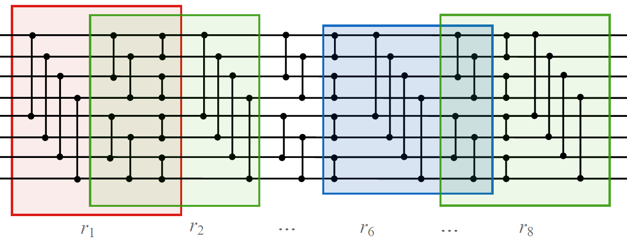
Our analysis of the spectral gap $\Delta_{\textrm{prop}}$ of the spacetime circuit propagation Hamiltonian begins with the standard mapping from $H_{\textrm{prop}}$ to a a Markov chain transition matrix $P$. ⁵⁵ 5 The re-scaled Hamiltonian $H_{\textrm{prop}}/\|H_{\textrm{prop}}\|$ is unitarily equivalent to a normalized graph Laplacian $\mathcal{L}$ for the graph with vertices corresponding to valid time configurations and edges corresponding to local gate updates on those time configurations. $P$ is the transition matrix for the random walk on this graph, which is obtained from $I-\mathcal{L}$ by a similarity transformation. The point is that these mappings provide an algebraic relation between $\Delta_{\textrm{prop}}$ and $\Delta_{P}$. To analyze the latter, we apply a Markov chain decomposition method due to Madras and Randall [MR02], which is used to split the Markov chain and its state space into pieces that are easier to analyze individually. For our decomposition of choice these pieces come in several closely related variants, which all essentially correspond to the set of time configurations contained within the final phase of a bitonic sorting circuit (as shown in Figure 3 for 8 lanes) which we call a bitonic block. As described in Appendix A, an arbitrary circuit consisting of 2-local gates can be transformed into a sequence of consecutive bitonic blocks, with at most a polylogarithmic factor of blow up in the depth.

After dividing the set of valid time configurations $\Omega$ (the state space of the Markov chain) into subsets $\Omega_{i}$ of configurations confined to bitonic blocks of the form illustrated in Figure 3, the subsets will form a quasi-linear chain in the sense that $\Omega_{i}$ and $\Omega_{j}$ have nonempty intersections when $|i-j|\leqslant\log n$. To apply the decomposition method we need to analyze (1) the spectral gap of the restricted Markov chains $P_{i}$ that are confined to stay within each of the subsets $\Omega_{i}$, and (2) the spectral gap of an aggregate Markov chain $\overline{P}$ that moves between the blocks based on transition probabilities related to the size of the intersections of the blocks.

As suggested by its quasi-linear connectivity, the spectral gap of the aggregate chain can be lower bounded using Cheeger’s inequality in similar manner as is done for the path graph Laplacian. The main technical challenge is to accurately compute the transition probabilities $\overline{P}(i,j)=\pi(\Omega_{i}\cap\Omega_{j})/\left(\Theta\pi(\Omega_{i})\right)$, which involve the ratio of the number of configurations within each of the blocks to the number within the pairwise intersections, $|\Omega_{i}\cap\Omega_{j}|/|\Omega_{i}|$, as well as the maximum number of blocks $\Theta$ that can contain any particular time configuration. In Appendix A, we develop a recurrence relation to exactly count these configurations and show that the former is constant for consecutive blocks (and decays doubly exponentially with $|i-j|$ for longer distance transitions), and the latter is logarithmic in $n$. Using asymptotic properties of the recurrence relation we show that the transition probabilities between $i,i+1$ are equal to $(\phi\log n)^{-1}$, where $\phi=(1+\sqrt{5})/2$ is the golden ratio. If there are $m$ blocks in total so that the length of the path is $m$, we use Cheeger’s inequality to show that the spectral gap $\Delta_{\overline{P}}$ of the aggregate chain satisfies

Turning to the analysis of the restricted chains $P_{i}$, we present the discovery of a surprising and beautiful connection between valid time configurations of architectures of the form shown in Figure 2 with combinatorial structures known as dyadic tilings [JRS02]. Dyadic tilings are tilings of the unit square by equal-area dyadic rectangles, which are rectangles of the form $[a2^{-s},(a+1)2^{-s}]\times[b2^{-t},(b+1)2^{-t}]$, where $a,b,s,t$ are nonnegative integers. These tilings have a natural recursive characterization: beginning from the unit square, draw a line that is either a horizontal or vertical bisector. This divides the square into two rectangles, and in each of these one chooses a horizontal or vertical bisector, and so on. After $\ell=\log(n)$ such recursive steps one obtains a dyadic tiling of rank $\ell$ with a total of $n$ dyadic rectangles, each with area $1/n$. Some examples are given in Figure 5.

For a spacetime circuit with $n$ qubits, we choose the blocks $\Omega_{i}$ in the decomposition so that for each block there is an exact bijection between the time configurations within the block and the set of equal-area dyadic tilings of rank $\ell=\log n$. Moreover, it turns out that the natural Markov chain on time configurations can also be mapped onto a previously defined Markov chain for dyadic tilings called the edge-flip chain. This Markov chain selects a rectangle of area $1/n$ in the current dyadic tiling and one of its four edges at random, and flips this edge if the result would be another dyadic tiling. The correspondence is described in Figure 6.

The mixing time of this edge flip chain was an open problem for over a decade, but has recently been the subject of a tour de force analysis that establishes an upper bound on the mixing time that is polynomial in $n$. Adapting these results using our bijection between these Markov chains yields

where the value of the exponent can be taken to be $\log(17)=4.087\ldots$. Once (1.5) and (1.6) are established, we combine them according to the decomposition result,

which is an inverse polynomial lower bound on the gap. The circuit propagation Hamiltonian is equivalent to the Markov chain $P$ scaled by a factor of $n$, and so we obtain $\Delta_{\textrm{prop}}=\widetilde{\Omega}(n^{-3.09})$. Finally, using the version of the spacetime Hamiltonian with circular time we show that every state in the code space has overlap $1/\polylog(n)$ with the input terms and so the geometrical lemma yields a gap of $\widetilde{\Omega}(n^{-3.09})$ for the full code Hamiltonian.

Here we present the formal definition of an approximate QLDPC code.

The first condition of the above definition enforces the locality and sparsity conditions of the approximate QLDPC code. The second condition enforces that the code is the ground space of a frustration-free local Hamiltonian. The third condition corresponds to the approximate error-correcting condition, where we only require that the decoded state is close to the original state (i.e., we no longer insist that $\mathrm{Rec}\circ\mathcal{E}\circ\mathrm{Enc}$ is exactly the identity channel). Although there are few results on approximate quantum error-correcting codes, we do know that relaxing the exact decoding condition yields codes with properties that cannot be achieved using exact codes [LNCY97, BO10].

We establish some notational conventions for parallel quantum circuits.

Consider the following model of depth $D$ circuits on $n$ qubits. The circuit $C$ consists of $D$ layers $L_{1},\ldots,L_{D}$. In each layer $L_{t}$ for $1\leqslant t\leqslant D$, the $n$ qubits are partitioned into $n/2$ disjoint pairs $\{(p,q)\}$, and a two-qubit gate $U_{t}(p,q)$ acts on the qubit pair $(p,q)$. Layer $L_{1}$ is applied first, then layer $L_{2}$, and so on. The unitary corresponding to circuit $C$ is

where the product is written from right to left. In other words, the unitary $\bigotimes_{(p_{1},q_{1})\in L_{1}}U_{1}[p_{1},q_{1}]$ is the rightmost factor, followed by $\bigotimes_{(p_{2},q_{2})\in L_{2}}U_{2}[p_{2},q_{2}]$, and so on.

As mentioned in the introduction, we use a small variant of the spacetime circuit Hamiltonian of Brueckmann and Terhal [BT14] to create our code Hamiltonian. In this section, we present the spacetime construction for general depth $D$ circuits. In Section 3, we will describe the specific circuit that we will use for our code Hamiltonian.

Let $D$ be an even integer and let $C$ be an $n$-qubit circuit of depth $D$ where $L_{1},\ldots,L_{D}$ be the $D$ layers of $C$, where each $L_{t}$ is a set of $n/2$ two-qubit gates⁶⁶ 6 By padding with identity gates, we can assume without loss of generality that every layer has exactly $n/2$ two-qubit gates. $U_{t}[p,q]$ acting on disjoint pairs of qubits $\{(p,q)\}$. We assume that $C$ is a “circular” circuit; in other words, that it is equivalent to the identity circuit.

We let $H_{circuit}[C]$ denote the circular spacetime circuit Hamiltonian corresponding to the circular circuit $C$. Let $X\stackrel{{\scriptstyle\mbox{\tiny def}}}{{=}}\frac{D-2}{2}$. The Hamiltonian is defined on $n(1+X+1)=n(X+2)$ qubits, which is divided into three classes of registers: (1) data registers ${\mathsf{S}}_{1},\ldots,{\mathsf{S}}_{n}$, (2) clock registers ${\mathsf{C}}_{1},\ldots,{\mathsf{C}}_{n}$, and (3) flag registers ${\mathsf{F}}_{1},\ldots,{\mathsf{F}}_{n}$.

The data register ${\mathsf{S}}_{i}$ is a qubit register that corresponds to the $i$-th qubit that the circuit $C$ acts on. The flag register ${\mathsf{F}}_{i}$ is a qubit register that indicates whether the $i$-th qubit’s local clock is in the “forward phase” or the “backward phase”; this denotes which half (first or second) of clock states the clock is in. The clock register ${\mathsf{C}}_{i}$ consists of $X$ qubits and indicates the local time of the $i$-th data qubit (within the forward phase or the backward phase). The valid clock states for register ${\mathsf{C}}_{i}$ are $\{|1^{j}0^{X-j}\rangle\}$ for $0\leqslant j\leqslant X$ (i.e. a domain wall clock).

Following Brueckmann and Terhal [BT14], the flag register combined with the clock register allows us to put our qubit clocks “on a circle”: we index time from $0$ to $2X+1=D-1$, and we identify time $t=D$ with $t=0$. We encode time steps $t$ according to the following convention. For notational convenience, we let the register ${\mathsf{T}}_{i}$ (for “time register”) denote the union of ${\mathsf{F}}_{i}$ and ${\mathsf{C}}_{i}$.

In other words, the time register evolves in the following way:

Notice that in any transition from $|t\rangle_{{\mathsf{T}}_{i}}$ to $|t+1\rangle_{{\mathsf{T}}_{i}}$, there is at most one qubit being flipped.

For the remainder of this section we fix a circuit $C$ and assume it fixed. The spacetime Hamiltonian $H_{circuit}[C]$ is defined as

The terms $H_{clock}$, $H_{init}$, $H_{prop}$, and $H_{causal}$ are defined as follows:

(1) $H_{clock}$:

The term $H_{clock}$ enforces that all the clock registers are encoded as described above. We write $H_{clock}=\sum_{i=1}^{n}H_{clock}[i]$ where

$$H_{clock}[i]=\sum_{j=1}^{D-1}\Pi_{{\mathsf{C}}_{i,j}{\mathsf{C}}_{i,j+1}}^{(01)}.$$

(2.9)

This enforces that the register ${\mathsf{C}}_{i}$ encodes a domain wall.

(2) $H_{init}$:

The initialization term is defined as $H_{init}=\sum_{i=k+1}^{n}H_{init}[i]$ for some integer $1\leqslant k\leqslant n$, ⁷⁷ 7 In our case, $k$ will eventually be the number of logical qubits. where

$$H_{init}[i]=\Pi_{{\mathsf{C}}_{i,0}}^{(1)}\otimes\Pi_{{\mathsf{S}}_{i}}^{(1)}.$$

(2.10)

This term checks that the last $n-k$ qubits are in the state $|0\rangle$ when their corresponding time registers are in state $|0\rangle_{{\mathsf{T}}_{i}}$ or $|2X+1\rangle_{{\mathsf{T}}_{i}}$. We only need to check one bit of the time register ${\mathsf{T}}_{i}$ because of the previous set of terms enforcing that the clock is a domain wall.

(3) $H_{prop}$:

The propagation term $H_{prop}$ is defined to be $H_{prop}=\sum_{t=0}^{D-1}\sum_{(p,q)\in L_{t}}H_{t}[p,q]$, where

	$\displaystyle H_{t}[p,q]$	$\displaystyle=\frac{1}{2}\Big[\left(A_{t,t}[p,q]+A_{t+1,t+1}[p,q]\right)\otimes\mathop{\mathds{1}}\!\mathinner{}$		(2.11)
		$\displaystyle-A_{t+1,t}[p,q]\otimes U_{t}[p,q]-A_{t,t+1}[p,q]\otimes(U_{t}[p,q])^{\dagger}\Big]$

	$\displaystyle\text{and }A_{t,t^{\prime}}[p,q]$	$\displaystyle=|u_{t}[p]\rangle\!\langle u_{t^{\prime}}[p]|\otimes|u_{t}[q]\rangle\!\langle u_{t^{\prime}}[q]|,$		(2.12)
	$\displaystyle|u_{t}[p]\rangle$	$\displaystyle=\begin{cases}\mathop{\mathds{1}}\!\mathinner{}\otimes|0\rangle_{{\mathsf{F}}_{p}}|1\rangle_{{\mathsf{C}}_{p,t}}|0\rangle_{{\mathsf{C}}_{p,t+1}}&\text{if }0\leqslant t<X\\ \mathop{\mathds{1}}\!\mathinner{}\otimes|0\rangle_{{\mathsf{F}}_{p}}|1\rangle_{{\mathsf{C}}_{p,X}}&\text{if }t=X\\ \mathop{\mathds{1}}\!\mathinner{}\otimes|1\rangle_{{\mathsf{F}}_{p}}|1\rangle_{{\mathsf{C}}_{p,X}}&\text{if }t=X+1\\ \mathop{\mathds{1}}\!\mathinner{}\otimes|1\rangle_{{\mathsf{F}}_{p}}|1\rangle_{{\mathsf{C}}_{p,2X+1-t}}|0\rangle_{{\mathsf{C}}_{p,2X+2-t}}&\text{if }X+1\leqslant t\leqslant 2X+1.\end{cases}$		(2.13)

Here, $|u_{t}[p]\rangle$ is the tensor product of a state on the specified qubits and the identity operator on all unspecified qubits. This term enforces the agreement of slices of the superposition corresponding to two time configurations differing by a gate with respect to the unitary $U_{t}[p,q]$. Because of the $H_{clock}$ terms, the checks only require looking at a few qubits of the time registers⁸⁸ 8 In effect, $|u_{t}[p]\rangle$ is the minimal description of $|t\rangle_{{\mathsf{T}}_{p}}$ given that the state is a ground-state of $H_{clock}$..

(4) $H_{causal}$:

The term $H_{causal}$ is used to enforce causality meaning that the superposition is only over valid time configurations (see Definition 3.4). At a high level, a time configuration ${\bm{\tau}}=(t_{1},\ldots,t_{n})$ is valid if and only if for all pairs of qubits $(p,q)$ sharing a gate in layer $L_{t}$, both clocks $t_{p}$ and $t_{q}$ are $\leqslant t$ or $>t$. This is, however, complicated by the circularity of time imposed in this particular construction as “all clocks are both ahead and behind any particular $t$”. In reality, we require the more complicated definition: for all pairs of qubits $(p,q)$ sharing gates in layers $L_{t_{a}}$ and $L_{t_{b}}$ for $t_{a}<t_{b}$, either $t_{p},t_{q}$ are both $\in[t_{a},t_{b})$ or are both $\notin[t_{a},t_{b})$.

Let $C_{p}$ be the set of qubits $q$ which interact with qubit $p$.

$$H_{causal}=\sum_{p=1}^{n}\sum_{q\in C_{p}}H_{causal}[p,q]$$

(2.14)

where $H_{causal}[p,q]$ is defined as follows. Let $t^{(1)}<t^{(2)}<\ldots<t^{(f)}$ be the times at which $p$ and $q$ share a gate. Then,

$$H_{causal}[p,q]=\sum_{j=1}^{f}\sum_{t_{p}=t^{(j)}}^{t^{(j+1)}-1}A_{t_{p},t_{p}}[p]\otimes B_{t^{(j)},t^{(j+1)}}[q]$$

(2.15)

where $B_{t,t^{\prime}}[q]$ is a projector ensuring that qubit $t_{q}$ is between $t$ and $t^{\prime}$ (respecting circularity)⁹⁹ 9 By this we mean that if $t<t^{\prime}$, the projector is onto the set $\{t,\ldots,t^{\prime}-1\}$. If $t^{\prime}<t$, then the projector is onto the set $\{t,\ldots,X\}\cup\{0,\ldots,t^{\prime}-1\}$.. Therefore, we verify that qubit $q$ is valid with respect to qubit $p$. The definition of $B_{t,t^{\prime}}[q]$ is case dependent.

Case 1

If $0\leqslant t,t^{\prime}\leqslant X$. In this case, the flag qubit must be $|0\rangle_{{\mathsf{F}}_{q}}$. Furthermore, ${\mathsf{C}}_{q,t}$ must be $|1\rangle$ and ${\mathsf{C}}_{q,t^{\prime}}$ must be $|0\rangle$. Therefore,

$$B_{t,t^{\prime}}[q]=\Pi_{{\mathsf{F}}_{q}}^{(0)}\Pi_{{\mathsf{C}}_{q,t}}^{(1)}\Pi_{{\mathsf{C}}_{q,t^{\prime}}}^{(0)}.$$

(2.16)

Case 2

If $X+1\leqslant t,t^{\prime}\leqslant 2X+1$. This is the similar except the flag is flipped. Hence,

$$B_{t,t^{\prime}}[q]=\Pi_{{\mathsf{F}}_{q}}^{(1)}\Pi_{{\mathsf{C}}_{q,2X+2-t^{\prime}}}^{(1)}\Pi_{{\mathsf{C}}_{q,2X+2-t}}^{(0)}.$$

(2.17)

Case 3

If $0\leqslant t\leqslant X$ and $X+1\leqslant t^{\prime}\leqslant 2X+1$. In this case, the flag qubit may be different. However, we can write the projector as the sum of the two projectors for the different flags.

$$B_{t,t^{\prime}}[q]=\Pi_{{\mathsf{F}}_{q}}^{(0)}\Pi_{{\mathsf{C}}_{q,t}}^{(1)}+\Pi_{{\mathsf{F}}_{q}}^{(1)}\Pi_{{\mathsf{C}}_{q,2X+2-t^{\prime}}}^{(1)}.$$

(2.18)

Case 4

If $0\leqslant t^{\prime}\leqslant X$ and $X+1\leqslant t\leqslant 2X+1$. This is similar except again the flag is flipped. Hence,

$$B_{t,t^{\prime}}[q]=\Pi_{{\mathsf{F}}_{q}}^{(0)}\Pi_{{\mathsf{C}}_{q,t^{\prime}}}^{(0)}+\Pi_{{\mathsf{F}}_{q}}^{(1)}\Pi_{{\mathsf{C}}_{q,2X+2-t}}^{(0)}.$$

(2.19)

In this section, we describe a class of circuits called bitonic sorting networks. These are parallel circuits, devised by Batcher [Bat68], that are used to efficiently sort data arrays. Specifically, these are circuits acting on $n$ elements, with depth $\mathcal{O}(\log^{2}n)$. In each layer of the circuit, pairs of elements are compared and swapped. Equivalently, for every permutation $\pi$ on $n$ elements, there is a bitonic sorting network consisting of SWAP and identity gates that implements $\pi$.

Bitonic sorting networks will be a crucial component of our code construction, as we use them to “uniformize” the random Brown-Fawzi encoding circuits before applying the spacetime circuit Hamiltonian construction. The uniformity of the resulting circuits will be the key ingredient that allows us to analyze the spectral gap of the Hamiltonian.

For this paper, we will be interested in the architecture (i.e. the wiring and gate structure) of the bitonic sorting circuit. A bitonic sorting architecture consists of smaller sub-architectures, called bitonic blocks.

We will use the notation $\mathcal{B}_{\ell}^{\times r}$ for the product (i.e. concatenation) of $r$ bitonic blocks $\mathcal{B}_{\ell}$. To simplify the analysis, we can insert additional layers of identity gates so that the circuit architecture is $\mathcal{B}_{\ell}^{\times\ell}$; this at most doubles the size of the circuit. Therefore, we can make the following statement:

We now present a general method for encoding depth $D$ circuits $C$ into a spacetime circuit Hamiltonian, in a way that allows us to give a good lower bound on the spectral gap. Let $C$ denote a circuit of depth $D$ consisting of layers $L_{1},\ldots,L_{D}$, where each $L_{t}$ is a set of $n/2$ two-qubit gates.

We preprocess the circuit $C$ in multiple steps to obtain a slightly larger-depth circuit $C^{\prime}$. We “uniformize” the circuit using bitonic sorting networks described in the previous section. The circuit $C$ will not, in general, correspond to nearest-neighbor interactions in small dimension. We add bitonic sorting networks in between each layer $L_{t}$ of $C$ to ensure that all the Clifford gates act on adjacent qubits. Because of the regular structure of the sorting networks, the resulting circuit will consist of nearest-neighbor interactions on a hypercube of dimension $\ell=\log n$.

More formally, we do the following: label the qubits using $\{1,\ldots,n\}$. In a layer $L_{t}$ of $C$ for $1\leqslant t\leqslant D$, a qubit $q$ is generally not paired with a neighboring qubit $q-1$ or $q+1$. Instead, there is some permutation $\pi_{t}$ on $n$ qubits that maps the pairs $\{(1,2),(2,3),\ldots,(n-1,n)\}$ to the pairs $L_{t}=\{(p,q)\}$. Let $\pi_{t}(L_{t})$ denote the layer where all the qubits are permuted by $\pi_{t}$, and all the gates in $L_{t}$ now act on consecutive qubits.

By Lemma 2.10, there exists a circuit $B_{\pi_{t}}$ with the architecture $\mathcal{B}_{\ell}^{\times\ell}$ for $\ell=\log n$ that implements the permutation $\pi_{t}$. Replace each layer $L_{t}$ in $C$ by the following subcircuit $K_{t}$: first apply $B_{\pi_{t}{\pi_{t}}^{-1}}$ and then apply the layer $\pi_{t}(L_{t})$. Since the last layer of $B_{\pi_{t}{\pi_{t}}^{-1}}$ and $\pi_{t}(L_{t})$ have the same architecture, we can merge the gates into a single layer. Here we assume $\pi_{0}=\mathop{\mathds{1}}\!\mathinner{}$.

The final $C^{\prime}$ is the composition of the subcircuits $K_{1},K_{2},\ldots,K_{D_{1}}$, yielding a depth $\mathcal{O}(D\log^{2}n)$ circuit. Note that by induction, circuit $C^{\prime}$ is exactly equivalent to the original circuit $C$. Notice that each subcircuit $K_{t}$ can be implemented as nearest-neighbor gates on a hypercube of dimension $\log n$, and thus the same holds for $C^{\prime}$ as well.

References

- [AAV13] Dorit Aharonov, Itai Arad, and Thomas Vidick. Guest column: the quantum PCP conjecture. ACM SIGACT news, 44(2):47–79, 2013.
- [ADH15] Ahmed Almheiri, Xi Dong, and Daniel Harlow. Bulk locality and quantum error correction in AdS/CFT. Journal of High Energy Physics, 2015(4):163, 2015.
- [AE15] Dorit Aharonov and Lior Eldar. Quantum locally testable codes. SIAM Journal on Computing, 44(5):1230–1262, 2015.
- [AVDK+08] Dorit Aharonov, Wim Van Dam, Julia Kempe, Zeph Landau, Seth Lloyd, and Oded Regev. Adiabatic quantum computation is equivalent to standard quantum computation. SIAM review, 50(4):755–787, 2008.
- [AZ18] Dorit Aharonov and Leo Zhou. On gap-simulation of Hamiltonians and the impossibility of quantum degree-reduction. arXiv preprint arXiv:1804.11084, 2018.
- [Bat68] K. E. Batcher. Sorting networks and their applications. In Proceedings of the April 30–May 2, 1968, Spring Joint Computer Conference, AFIPS ’68 (Spring), pages 307–314, New York, NY, USA, 1968. ACM.
- [BC18] Johannes Bausch and Elizabeth Crosson. Analysis and limitations of modified circuit-to-Hamiltonian constructions. Quantum, 2:94, September 2018.
- [BCŞB17] Fernando GSL Brandao, Elizabeth Crosson, M Burak Şahinoğlu, and John Bowen. Quantum error correcting codes in eigenstates of translation-invariant spin chains. arXiv preprint arXiv:1710.04631, 2017.
- [BF13] Winton Brown and Omar Fawzi. Short random circuits define good quantum error correcting codes. In Information Theory Proceedings (ISIT), 2013 IEEE International Symposium on, pages 346–350. IEEE, 2013.
- [BFHS17] Dave Bacon, Steven T Flammia, Aram W Harrow, and Jonathan Shi. Sparse quantum codes from quantum circuits. IEEE Transactions on Information Theory, 63(4):2464–2479, 2017.
- [BH14] Sergey Bravyi and Matthew B Hastings. Homological product codes. In Proceedings of the forty-sixth annual ACM symposium on Theory of computing, pages 273–282. ACM, 2014.
- [BHM10] Sergey Bravyi, Matthew B Hastings, and Spyridon Michalakis. Topological quantum order: stability under local perturbations. Journal of mathematical physics, 51(9):093512, 2010.
- [BO10] Cédric Bény and Ognyan Oreshkov. General conditions for approximate quantum error correction and near-optimal recovery channels. Physical review letters, 104(12):120501, 2010.
- [BT09] Sergey Bravyi and Barbara Terhal. A no-go theorem for a two-dimensional self-correcting quantum memory based on stabilizer codes. New Journal of Physics, 11(4):043029, 2009.
- [BT14] Nikolas P Breuckmann and Barbara M Terhal. Space-time circuit-to-Hamiltonian construction and its applications. Journal of Physics A: Mathematical and Theoretical, 47(19):195304, 2014.
- [CB17] Elizabeth Crosson and John Bowen. Quantum ground state isoperimetric inequalities for the energy spectrum of local Hamiltonians. arXiv preprint arXiv:1703.10133, 2017.
- [CGS05] Claude Crépeau, Daniel Gottesman, and Adam Smith. Approximate quantum error-correcting codes and secret sharing schemes. In Proceedings of the 24th annual international conference on Theory and Applications of Cryptographic Techniques, pages 285–301. Springer-Verlag, 2005.
- [CLN18] Libor Caha, Zeph Landau, and Daniel Nagaj. Clocks in Feynman’s computer and Kitaev’s local Hamiltonian: Bias, gaps, idling, and pulse tuning. Physical Review A, 97(6):062306, 2018.
- [CLS17] Sarah Cannon, David A. Levin, and Alexandre Stauffer. Polynomial Mixing of the Edge-Flip Markov Chain for Unbiased Dyadic Tilings. In Approximation, Randomization, and Combinatorial Optimization. Algorithms and Techniques (APPROX/RANDOM 2017), volume 81 of Leibniz International Proceedings in Informatics (LIPIcs), pages 34:1–34:21, 2017.
- [CS96] A Robert Calderbank and Peter W Shor. Good quantum error-correcting codes exist. Physical Review A, 54(2):1098, 1996.
- [EH17] Lior Eldar and Aram W Harrow. Local Hamiltonians whose ground states are hard to approximate. In Foundations of Computer Science (FOCS), 2017 IEEE 58th Annual Symposium on, pages 427–438. IEEE, 2017.
- [EOT16] Lior Eldar, Maris Ozols, and Kevin F Thompson. The need for structure in quantum LDPC codes. arXiv preprint arXiv:1610.07478, 2016.
- [FHKK17] Steven T Flammia, Jeongwan Haah, Michael J Kastoryano, and Isaac H Kim. Limits on the storage of quantum information in a volume of space. Quantum, 1:4, 2017.
- [FML02] Michael H Freedman, David A Meyer, and Feng Luo. Z2-systolic freedom and quantum codes. Mathematics of quantum computation, Chapman & Hall/CRC, pages 287–320, 2002.
- [Gal63] Robert G. Gallager. Low-density parity-check codes, 1963.
- [GGC18] Carlos E González-Guillén and Toby S Cubitt. History-state Hamiltonians are critical. arXiv preprint arXiv:1810.06528, 2018.
- [Got13] Daniel Gottesman. Fault-tolerant quantum computation with constant overhead. arXiv preprint arXiv:1310.2984, 2013.
- [GS13] Anand Ganti and Rolando Somma. On the gap of Hamiltonians for the adiabatic simulation of quantum circuits. International Journal of Quantum Information, 11(07):1350063, 2013.
- [GTV15] David Gosset, Barbara M. Terhal, and Anna Vershynina. Universal adiabatic quantum computation via the space-time circuit-to-Hamiltonian construction. Phys. Rev. Lett., 114:140501, Apr 2015.
- [Has13] Matthew B Hastings. Trivial low energy states for commuting Hamiltonians, and the quantum PCP conjecture. Quantum Information & Computation, 13(5-6):393–429, 2013.
- [Has17a] Mathew B Hastings. Weight reduction for quantum codes. Quantum Information & Computation, 17(15-16):1307–1334, 2017.
- [Has17b] Matthew B Hastings. Quantum codes from high-dimensional manifolds. In LIPIcs-Leibniz International Proceedings in Informatics, volume 67, 2017.
- [JRS02] Svante Janson, Dana Randall, and Joel Spencer. Random dyadic tilings of the unit square. 21:225–251, 10 2002.
- [Kit03] A Yu Kitaev. Fault-tolerant quantum computation by anyons. Annals of Physics, 303(1):2–30, 2003.
- [KL96] Emanuel Knill and Raymond Laflamme. A theory of quantum error-correcting codes. 1996.
- [KN97] Tohru Koma and Bruno Nachtergaele. The spectral gap of the ferromagnetic XXZ-chain. Letters in Mathematical Physics, 40(1):1–16, 1997.
- [LBF17] Yi-Chan Lee, Courtney G Brell, and Steven T Flammia. Topological quantum error correction in the Kitaev honeycomb model. Journal of Statistical Mechanics: Theory and Experiment, 2017(8):083106, 2017.
- [LNCY97] Debbie W Leung, Michael A Nielsen, Isaac L Chuang, and Yoshihisa Yamamoto. Approximate quantum error correction can lead to better codes. Physical Review A, 56(4):2567, 1997.
- [LP17] David A Levin and Yuval Peres. Markov chains and mixing times, volume 107. American Mathematical Soc., 2017.
- [LST17] Seth Lloyd, Peter Shor, and Kevin Thompson. polylog-LDPC capacity achieving codes for the noisy quantum erasure channel. arXiv preprint arXiv:1703.00382, 2017.
- [LSV02] Jeffrey C Lagarias, Joel H Spencer, and Jade P Vinson. Counting dyadic equipartitions of the unit square. Discrete mathematics, 257(2-3):481–499, 2002.
- [LT16] Seth Lloyd and Barbara M Terhal. Adiabatic and Hamiltonian computing on a 2d lattice with simple two-qubit interactions. New Journal of Physics, 18(2):023042, 2016.
- [MLM07] Ari Mizel, Daniel A Lidar, and Morgan Mitchell. Simple proof of equivalence between adiabatic quantum computation and the circuit model. Physical review letters, 99(7):070502, 2007.
- [MR02] Neal Madras and Dana Randall. Markov chain decomposition for convergence rate analysis. Ann. Appl. Probab., 12(2):581–606, 05 2002.
- [MW05] Chris Marriott and John Watrous. Quantum Arthur–Merlin games. Computational Complexity, 14(2):122–152, 2005.
- [NVY18] Chinmay Nirkhe, Umesh Vazirani, and Henry Yuen. Approximate Low-Weight Check Codes and Circuit Lower Bounds for Noisy Ground States. In 45th International Colloquium on Automata, Languages, and Programming (ICALP 2018), volume 107 of Leibniz International Proceedings in Informatics (LIPIcs), pages 91:1–91:11, 2018.
- [Ste96] Andrew Steane. Multiple-particle interference and quantum error correction. Proc. R. Soc. Lond. A, 452(1954):2551–2577, 1996.
- [TZ14] Jean-Pierre Tillich and Gilles Zémor. Quantum LDPC codes with positive rate and minimum distance proportional to the square root of the blocklength. IEEE Transactions on Information Theory, 60(2):1193–1202, 2014.
Appendix A Partially applied configurations of a bitonic sorting circuit
In this Appendix, we provide the mathematical foundations required for analyzing the spectral gap of the Hamiltonian and generating the encoding circuit. We explore the properties of the bitonic block [Bat68] (see Definition 2.7) and prove results about the space of valid configurations of partial computations of a bitonic block (see Definition 3.4).
A.1 Configurations and width
We study the structure and combinatorics of the valid configurations (see Definition 3.4). One can think of a valid partial configuration as being represented visually on the architecture as a string which partitions the architecture into two halves: gates that have and have not been applied. Depending on the configuration of the circuit in question, there is a maximum width, a number of layers, that such a string can have.
Definition A.1.
The width of a partial configuration is