A framework for quantum-secure device-independent randomness expansion
Abstract
A device-independent randomness expansion protocol aims to take an initial random seed and generate a longer one without relying on details of how the devices operate for security. A large amount of work to date has focussed on a particular protocol based on spot-checking devices using the CHSH inequality. Here we show how to derive randomness expansion rates for a wide range of protocols, with security against a quantum adversary. Our technique uses semidefinite programming and a recent improvement of the entropy accumulation theorem. To support the work and facilitate its use, we provide code that can generate lower bounds on the amount of randomness that can be output based on the measured quantities in the protocol. As an application, we give a protocol that robustly generates up to two bits of randomness per entangled qubit pair, which is twice that established in existing analyses of the spot-checking CHSH protocol in the low noise regime.
1 Introduction
Random numbers are an essential resource in the information processing era, finding applications in gaming, simulations and cryptography. Cryptographic protocols are frequently built upon an assumption of access to a private random seed. Using poor-quality randomness can be fatal to the security of the protocol (see, e.g., [1]). Thus, in order to adhere to these standard protocol assumptions, it is imperative that we are able to certify the generation of private random numbers.
The intrinsic randomness of quantum theory provides a natural mechanism with which we can generate random numbers: a simple source of perfectly random bits could be a device that prepares a eigenstate and then measures . However, the use of such a source comes with a significant caveat: the internal mechanisms of the preparation and measurement devices must be well-characterized and kept stable throughout their use. Any mismatch between the characterization and how the device operates in practice may be an exploitable weakness in the hands of a smart enough adversary; such mismatches have been used to compromise commercially available quantum key distribution (QKD) systems (see e.g., [2]).
While weaknesses caused by mismatches may be mitigated by increasingly detailed descriptions of the quantum devices, generating such descriptions rapidly becomes unwieldy and remaining vulnerabilities can be difficult to detect. This is reminiscent of the situation in modern software engineering where security flaws are frequently discovered and patched. Fixing hardware vulnerabilities, such as those exploited in the aforementioned QKD attacks, can be more difficult logistically and economically.
Fortunately, quantum theory provides a means to address this problem. Going back to [3] and using an important insight of [4], device-independent quantum cryptography establishes security independently of the devices involved within a protocol, relying only on the validity of quantum theory and the imposition of certain no-signalling constraints between devices. Security is subsequently verified through the observation of non-local output statistics, which in turn act as witnesses to the inner workings of the devices. Limiting the number of initial assumptions greatly reduces the threat of side-channel attacks.
In this work we focus on the task of randomness expansion: a procedure wherein one attempts to transform a short private seed into a much larger (still private) source of uniform random bits. Randomness expansion in a device-independent setting was proposed in [5, 6] with further development and experimental testing following shortly after [7]. Subsequent work provided security proofs against classical adversaries [8, 9]. Security against quantum adversaries—who may share entanglement with the internal state of the device—came later [10, 11, 12], progressively increasing in noise-tolerance and generality, with the recently introduced entropy accumulation theorem (EAT) [13, 23], on which our work is based, providing asymptotically optimal rates [14, 15]. A new proof technique that is also asymptotically optimal has recently appeared [16].
In [14] the EAT was applied to the task of randomness expansion and a general entropy accumulation procedure was detailed. The security of the resulting randomness expansion protocol relies on the construction of a randomness bounding function (known as a min-tradeoff function) that characterizes the average entropy gain during the protocol. Unfortunately, the analysis in [14] applies only to protocols based on the CHSH inequality, and relies on some analytic steps that do not directly generalize to arbitrary protocols11 1 In particular, simplifications that arise due to the two party, two input, two output scenario being reducible to qubits.. However, as was also noted in [14], one could look to use the device-independent guessing probability (DIGP) [20, 21, 22] in conjunction with the semidefinite hierarchy [18, 19] to obtain computational constructions of the required min-tradeoff functions.
Here we detail a precise method for combining these semidefinite programming tools with the EAT to construct min-tradeoff functions. We then apply this construction to the task of randomness expansion to prove security of protocols based upon arbitrary nonlocal games. This includes protocols with arbitrary (but finite) numbers of inputs-outputs, as well as protocols based upon multiple Bell-inequalities [17]. It is worth noting that this construction could also be readily extended to multipartite scenarios although we do not discuss these in this work. Moreover, as this computational method takes the form of a semidefinite program these constructions are both computationally efficient and reliable, although at the cost of producing potentially suboptimal bounds. To accompany this work, we provide a code package (available at [24]) for the construction and analysis of these randomness expansion protocols.
In more detail, we give a template protocol, Protocol QRE, from which a user can develop their randomness expansion protocol. Given certain parameters chosen by a user, e.g., time constraints, choice of non-locality tests and security tolerances, the projected randomness expansion rates to be calculated. If these rates are unsatisfactory, then modifications to the protocol’s design can be made and the rates recalculated. As the computations can be done with a computationally efficient procedure, the user can optimize their protocol parameters to best fit their experimental setup. Once a choice of experimental design has been made, the resulting randomness expansion procedure can be performed. Subject to the protocol not aborting, this gives a certifiably private random bit-string.
We apply our technique to several example protocols. In particular, we look at randomness expansion using the complete empirical distribution as well as a simple extension of the CHSH protocol, showing noise-tolerant rates of up to two bits per entangled qubit pair, secure against quantum adversaries. Although means of generating two bits of randomness per entangled qubit pair have been considered before [25] to the best of our knowledge our work is the first to present a full protocol and prove that this rate can be robustly achieved taking into account finite statistics. The nonlocal game we use for this is related to that in [25]. We also compare the achievable rates for these protocols to the protocol presented in [14] which is based upon a direct von Neumann entropy bound. Our comparison demonstrates that some of the protocols from the framework are capable of achieving higher rates than the protocol of [14], in both the low and high noise regimes. Improved rates in the high noise regime are of particular importance when considering current experimental implementations, because of the difficulty of significantly violating the CHSH inequality while closing the detection loophole [26, 27, 28]. Additionally, we include in the appendices a full non-asymptotic account of input randomness necessary for running the protocols.
The paper is structured as follows: in Sec. 2 we introduce the material relevant for our construction. In Sec. 3 we detail the various components of our framework and present the template protocol with full security statements and proofs. We provide examples of several randomness expansion protocols built within our framework in Sec. 4 before concluding with some open problems in Sec. 5.
2 Preliminaries
2.1 General notation
Throughout this work, the calligraphic symbols , , and denote finite alphabets and we use the notational shorthand to denote the Cartesian product alphabet . We refer to a behaviour (or strategy) on these alphabets as some conditional probability distribution, with , which we view as a vector . That is, by denoting the set of canonical bases vectors of by , we write . We make the distinction between the vector and its elements through the use of boldface, i.e., . Throughout this work we assume that all conditional distributions obey the no-signalling constraints that is independent of and hence can be written and similarly . We denote the set of all no-signalling behaviours by . Given an alphabet we denote the set of all distributions over by , and given a sequence , with for each , we denote the frequency distribution induced by by
| (1) |
where is the Kronecker delta on the set .
We use the symbol to denote a Hilbert space, subscripting with system labels when helpful. For a system , we denote the set of positive semidefinite operators with unit trace acting on by and its subnormalized extension (i.e., the set that arises when the trace is restricted to be in the interval ) by (we extend the use of tildes to other sets to denote their subnormalized extensions). We refer to a state as a classical-quantum state (cq-state) on the joint system if it can be written in the form where is a set of orthonormal vectors in . Letting be an event on the alphabet , we define the conditional state (conditioned on the event ) by
| (2) |
We denote the identity operator of a system by . We write the natural logarithm as and the logarithm base as . The function is the sign function, mapping all positive numbers to , negative numbers to and to .
We say that a behaviour is quantum if its elements can be written in the form where and , are sets of POVMs; we denote the set of all quantum behaviours by . Additionally, we use to denote the subnormalized extension of this set.
Note that randomness expansion is a single-party protocol; there is one user who wishes to expand an initial private random string. However, that user may work with a bipartite setup in which they use two devices that are prevented from signalling to one another; in such a case we sometimes refer to Alice and Bob as the users of each device. Note though that, unlike in QKD, Alice and Bob are agents of the same party and are within the same laboratory. There may also be a dishonest party, Eve, trying to gain information about the random outputs.
2.2 Entropies and SDPs
The von Neumann entropy of is
| (3) |
For a bipartite state , we use the notation for and define the conditional von Neumann entropy of system given system when the joint system is in state by
| (4) |
In addition, for a tripartite system , the conditional mutual information between and given is defined by
We drop the state subscript whenever the state is clear from the context.
In this work it is useful to consider the conditional min-entropy [30] in its operational formulation [22]. Given a cq-state , the maximum probability with which an agent holding system can guess the outcome of a measurement on is
| (5) |
where the maximum is taken over all POVMs on system . Using this we can define the min-entropy of a classical system given quantum side information as
| (6) |
The final entropic quantity we consider is the -smooth min-entropy [31]. Given some and , the -smooth min-entropy is defined as the supremum of the min-entropy over all states -close to ,
| (7) |
where is the -ball centred at defined with respect to the purified trace distance [32]. For a thorough overview of smooth entropies and their properties we refer the reader to [33].
In the device-independent scenario we do not know the quantum states or measurements being performed. Instead, our entire knowledge about these must be inferred from the observed input-output behaviour of the devices used. In particular, observing correlations that violate a Bell inequality provides a coarse-grained characterization of the underlying system. In a device-independent protocol, the idea is to use only this to infer bounds on particular system quantities, e.g., the randomness present in the outputs. As formulated above, the guessing probability (5) is not a device-independent quantity because its computation requires knowing . However, the guessing probability can be reformulated in a device-independent way [34, 20, 21, 17] as we now explain.
Consider a tripartite system shared between two devices in the user’s lab and Eve. Because we are assuming an adversary limited by quantum theory, we can suppose that, upon receiving some inputs , the devices work by performing measurements and respectively, which give rise to some probability distribution , and overall state
where , and . Note that the user of the protocol is not aware of what the devices are doing.
Consider the best strategy for Eve to guess the value of using her system . She can perform a measurement on her system to try to distinguish (occurring with probability ). Denoting Eve’s POVM with outcomes in one-to-one correspondence with the values can take (say being the value corresponding to a best guess of )22 2 Without loss of generality we can assume Eve’s measurement has as many outcomes as what she is trying to guess., then given some values of and , Eve’s outcomes are distributed as , and her probability of guessing correctly is . Hence, the overall probability of guessing correctly given and for the quantum realisation of the statistics, , is
Note that the guessing probability depends on the inputs . In the protocols we consider later, there will only be one pair of inputs for which Eve is interested in guessing the outputs. We denote these inputs by and .
In the device-independent scenario, Eve can also optimize over all quantum states and measurements that could be used by the devices. However, she wants to do so while restricting the devices to obey certain relations which depend on the protocol (for example, the CHSH violation that could be observed by the user). For the moment, without specifying these relations precisely, call the set of quantum states and measurements obeying these relations . Hence, we seek
Because Eve’s measurement commutes with those of the devices, due to no signalling we can use Bayes’ rule to rewrite the optimization as33 3 This rewriting makes sense provided no information leaks to Eve during the protocol, which is reasonable for randomness expansion since it takes place in one secure lab.
With this rewriting it is evident that we can think about Eve’s strategy as follows: Eve randomly chooses a value of and then prepares the device according to that choice, i.e., trying to bias towards the values corresponding to the chosen .
We can hence write
where satisfies some relations (equivalent to the restriction to the set ) and for each . Provided the relations satisfied are linear, which we will henceforth assume, they can be expressed as a matrix equation and the whole optimization is a conic program (the set of un-normalized quantum-realisable distributions forms a convex cone). By writing as the subnormalized distribution the problem can be expressed as
| (8) | ||||||
Note that the normalisation condition, , is assumed to be contained within (or a consequence of) the conditions imposed by . For the particular sets of conditions that we impose later, normalization always follows.
Optimizing over the set of quantum correlations is a difficult problem, in part because the dimension of the quantum system achieving the optimum could be arbitrarily large. Because of this, we consider a computationally tractable relaxation of the problem, by instead optimizing over distributions within some level of the semidefinite hierarchy [18, 19]. We denote the level by . This relaxation of the problem takes the form of a semidefinite program that can be solved in an efficient manner, at the expense of possibly not obtaining the same optimum value. The corresponding relaxed program is
| (9) | ||||||
This program has a dual. In Appendix D we show that there is an alternative program with the same properties44 4 In particular, the weak duality statement holds. as the standard dual. To specify this, we define the set of valid constraint vectors at level by the set of vectors for which there exists such that .
The alternative dual then takes the form
| (10) | ||||||
with . Since the NPA hierarchy forms a sequence of outer approximations to the set of quantum correlations, , the relaxed guessing probability provides an upper bound on the true guessing probability, i.e., . Combined with (6), one can use the relaxed programs to compute valid device-independent lower bounds on .
Programs (9) and (10) are parameterized by a vector . We denote a feasible point of the dual program parameterized by by . Note that for our later analysis we only need to be a feasible point of the dual program, we do not require it to be optimal.55 5 An optimal choice of for (10) may not even exist.
2.3 Devices and nonlocal games
Device-independent protocols involve a series of interactions with some untrusted devices. A device refers to some physical system that receives classical inputs and produces classical outputs. Furthermore, we say that is untrusted if the mechanism by which produces the outputs from the inputs need not be characterized. During the protocol, the user interacts with their untrusted devices within the following scenario:66 6 One does not have to recreate this scenario exactly in order to perform the protocol. Instead, the given scenario establishes one situation in which the protocol remains secure (see Def. 2.2 for a precise definition of security).
- 1.
The protocol is performed within a secure lab from which information can be prevented from leaking.
- 2.
This lab can be partitioned into disconnected sites (one controlled by Alice and one by Bob).
- 3.
The user can send information freely between these sites without being overheard, while at the same time, they can prevent unwanted information transfer between the sites.77 7 In this work we need to ensure that the user’s devices are unable to communicate at certain points of the protocol (when Bell tests are being done), but not at others (e.g., when entanglement is being distributed). However, they should never be allowed to send any information outside the lab after the protocol begins.
- 4.
The user has two devices to which they can provide inputs (taken from alphabets and ) and receive outputs (from alphabets and ).
- 5.
These devices operate according to quantum theory, i.e., . Any eavesdropper is also limited by quantum theory88 8 In parts of this paper we allow the eavesdropper limited additional power—the bounds will then still apply if the eavesdropper is limited by quantum theory.. We use to denote the collection of devices (including any held by an eavesdropper) and refer to this as an untrusted device network.
- 6.
The user has an initial source of private random numbers and a trusted device for classical information processing.
One of the key advantages of a device-independent protocol is that because no assumptions are made on the inner workings of the devices used, the protocol checks that the devices are working sufficiently well on-the-fly. The protocols hence remain impervious to many side-channel attacks, malfunctioning devices or prior tampering. The idea behind their security is that by testing that the devices exhibit ‘nonlocal’ correlations, their internal workings are sufficiently restricted to enable the task at hand.
In this work, we formulate the testing of the devices through nonlocal games. A nonlocal game is initiated by a referee who sends the two players their own question chosen according to some distribution, . The players then respond with their answers chosen from and respectively. Using the predefined scoring rule , the referee then announces whether or not they won the game. The game is referred to as nonlocal because prior to receiving their questions, the players are separated and unable to communicate until they have given their answers. The question sets, answer sets, distribution and the scoring rule are all public knowledge. Moreover, the players are allowed to confer prior to the start of the game.
Definition 2.1:
Let and be finite sets. A (two-player) nonlocal game (on ) consists of a set of question pairs chosen according to some probability distribution , a set of answer pairs and a scoring function . A strategy for is a conditional distribution defined on the question and answer sets.
Remark 2.1:
We will abuse notation and use the symbol to refer to both the nonlocal game and the set of possible scores. I.e., we may refer to the players receiving a score . Furthermore, we denote the number of different scores by .
If the players play using the strategy , then this induces a frequency distribution over the set of possible scores. That is,
| (11) |
for each . The expected frequency distribution, , will be the figure of merit by which we evaluate the performance of our untrusted devices. We denote the set of possible frequency distributions achievable by the agents whilst playing according to quantum strategies by .
Example 2.1 (Extended CHSH game ):
The extended CHSH game has appeared already in the device-independent literature in the context of QKD (see, e.g., [35]). It extends the standard CHSH game to include a correlation check between one of Alice’s CHSH inputs and an additional input from Bob. It is defined by the question-answer sets , and , the scoring set and the scoring rule
| (12) |
The input distribution we consider is defined by for , and otherwise. This game is equivalent to choosing to play either the game or the game corresponding to checking the alignment of the inputs uniformly at random and then proceeding with the chosen game. The frequency distribution then tells us the relative frequencies with which we win each game. The motivation behind can be understood by considering a schematic of an ideal implementation on a bipartite qubit system as given in Fig. 1. If we observe the maximum winning probability for the CHSH game, as well as perfect alignment for the inputs , then the inputs should produce two perfectly uniform bits.
2.4 Device-independent randomness expansion protocols and their security
A device-independent randomness expansion protocol is a procedure by which one attempts to use a uniform, trusted seed, , to produce a longer uniform bit-string, , through repeated interactions with some untrusted devices. We consider so-called spot-checking protocols, which involve two round types: test-rounds, during which one attempts to produce certificates of nonlocality, and generation rounds in which a fixed input is given to the devices and the outputs are recorded. By choosing the rounds randomly according to a distribution heavily favouring generation rounds, we are able to reduce the size of the seed whilst sufficiently constraining the device’s behaviour, guaranteeing the presence of randomness in the outcomes (except with some small probability).
Using the setup described in Sec. 2.3, our template randomness expansion protocol consists of two main steps.
- 1.
Accumulation: In this phase the user repeatedly interacts with the separated devices. Each interaction is randomly chosen to be a generation round or a test round in a coordinated way using the initial random seed.99 9 For example, a central source of randomness could be used to choose the round type. This information could then be communicated to each party (in such a way that the devices do not learn this choice). On generation rounds the devices are provided with some fixed inputs , whereas during test rounds, the testing procedure specific to the protocol is followed. After many interactions, the recorded outputs are concatenated to give . Using the statistics collected during test rounds, a decision is made about whether to abort or not based on how close the observations are to some pre-defined expected device behaviour.
- 2.
Extraction: Subject to the protocol not aborting in the accumulation step, a quantum-proof randomness extractor is applied to . This maps the partially random to a shorter string that is the output of the protocol.
We define security of a randomness expansion protocol according to a composable definition [39, 40, 41, 42, 43]. Using composable security ensures that the output randomness can be used in any other application with only an arbitrarily small probability of it being distinguishable from perfect randomness. To make this more precise, consider a hypothetical device that outputs a string that is uniform and uncorrelated with any information held by an eavesdropper. In other words, it outputs , where is the maximally mixed state on qubits. The ideal protocol is defined as the protocol that involves first doing the real protocol, then, in the case of no abort, replacing the output with a string of the same length taken from the hypothetical device. The protocol is then said to be -secure ( is called the soundness error) if, when the user either implements the real or ideal protocol with probability , the maximum probability that a distinguisher can guess which is being implemented is at most . If is small, then the real and ideal protocols are virtually indistinguishable. Defining the ideal as above ensures that the real and ideal protocols can never be distinguished by whether or not they abort. We refer to [43] for further discussion of composability in a related context (that of QKD).
There is a second important parameter of any protocol, its completeness error, which is the probability that an ideal implementation of the protocol leads to an abort. It is important for a protocol to have a low completeness error in addition to a low soundness error since a protocol that always aborts is vacuously secure.
Definition 2.2:
Consider a randomness expansion protocol whose output is denoted by . Let be the event that the protocol does not abort. The protocol is an -randomness expansion protocol if it satisfies the following two conditions.
- 1.
Soundness:
(13) where is an arbitrary quantum register (which could have been entangled with the devices used at the start of the protocol), is the length of the output string and is the maximally mixed state on a system of dimension .
- 2.
Completeness: There exists a set of quantum states and measurements such that if the protocol is implemented using those
(14)
Although we use a composable security definition to ensure that any randomness output by the protocol can be used in any scenario, importantly, this may not apply if the devices used in the protocol are subsequently reused [44]. Thus, after the protocol the devices should be kept shielded and not reused until such time as the randomness generated no longer needs to be kept secure. How best to resolve this remains an open problem: the Supplemental Material of [44] presents candidate protocol modifications (and modifications to the notion of composability) that may circumvent such problems.
2.5 Entropy accumulation
In order to bound the smooth min entropy accumulated during the protocol we employ the EAT [13, 23]. Roughly speaking, the EAT says that this min-entropy is proportional to the number of rounds, up to square root correction factors. The proportionality constant is the single-round conditional von Neumann entropy optimized over all states that can give rise to the observed scores. In its full form, the EAT is an extension of the asymptotic equipartition property [45] to a particular non-i.i.d. regime. For the purposes of randomness expansion we only require a special case of the EAT, which we detail later in this section.
With the goal of maximising our entropic yield, we use the recently improved statement of the entropy accumulation theorem [23].1010 10 We discuss this EAT statement and compare it to alternatives in Appendix C. For completeness we present the relevant statements including the accumulation procedure (see also [15]).
2.5.1 The entropy accumulation procedure
The entropy accumulation procedure prescribes how the user interacts with their untrusted devices and collects data from them. Before beginning this procedure a nonlocal game that is compatible with the alphabets of the devices is selected.
A round within the entropy accumulation procedure consists of the user giving an input to each of their devices and recording the outputs. We use subscripts on random variables to indicate the round that they are associated with, i.e., are the random variables describing the joint device inputs for the round. In addition, boldface will be used to indicate that a random variable represents the concatenation over all rounds of the protocol, .
The accumulation procedure consists of separate interactions with the untrusted devices. We refer to a single interaction with the devices as a round. A round consists of the user selecting and supplying inputs to the devices, receiving outputs and recording this data. During the round, a random variable is sampled, for some fixed , indicating whether the round will be a generation round or a test round. With probability we have and the round is a generation round. During a generation round, the user supplies the respective devices with the fixed generation inputs , recording . They record the outputs received from the devices as and respectively and they record the round’s score as . With probability , and the round is a test round. During a test round, inputs are sampled according to the distribution specified by the chosen nonlocal game. The sampled inputs are fed to their respective devices and the outputs received are recorded as . The score is computed and recorded as . The transcript for round is the tuple . After rounds, the complete transcript for the accumulation procedure is . We denote by the set of possible values that can take, i.e. .
After the -round transcript has been obtained, the user looks to determine the performance of the untrusted devices and, in turn, certify a lower bound on the total entropy produced, . To this end, the user computes the empirical frequency distribution
| (15) |
Prior to the accumulation step, the user fixes some frequency distribution corresponding to an expected (or hoped for) behaviour. Should the devices behave in an i.i.d. manner according to , then concentration bounds tell us that the empirical frequency distribution should be close to . With this in mind, we define the event that the protocol does not abort by
| (16) |
where is a vector of confidence interval widths satisfying with all vector inequalities being interpreted as element-wise constraints.
2.5.2 The entropy accumulation theorem
To complete the protocol, uniform randomness needs to be extracted from the partially random outputs. Doing so requires the user to assume a lower bound on the smooth min-entropy (conditioned on any side information held by an adversary) contained in the devices’ outputs when the protocol does not abort. If is very small, then the assumption must be correct with near certainty. The EAT provides a method by which one can compute such a lower bound. Loosely, the EAT states that if the interaction between the honest parties occurs in a sequential manner (as described in Sec. 2.5.1), then with high probability the uncertainty an adversary has about the outputs is close to their total average uncertainty. As a mathematical statement it is a particular example of the more general phenomenon of concentration of measure (see [46] for a general overview). In order to state the EAT precisely, we first require a few definitions.
Definition 2.3 (EAT channels):
A set of EAT channels is a collection of trace-preserving and completely-positive maps such that for every :
- 1.
and are finite dimensional classical systems, is an arbitrary quantum system and is the output of a deterministic function of the classical registers and .
- 2.
For any initial state , the final state fulfils the Markov chain condition for every .
The EAT channels formalise the notion of interaction within the protocol. The first condition in Def. 2.3 specifies the nature of the information present within the protocol and, in particular, it restricts the honest parties’ inputs to their devices to be classical in nature. The arbitrary quantum register represents the quantum state stored by the separate devices after the round. The second condition specifies the sequential nature of the protocol. The channels describe the joint action of both devices and include the generation of the randomness needed to choose the settings. The Markov chain condition implies that the inputs to the devices presented by the honest parties are conditionally independent of the previous outputs they have received. Note that by using a trusted private seed to choose the inputs and supplying the inputs sequentially (as is done in Sec. 2.5.1), this condition will be satisfied.1111 11 A public seed can also be used if the Markov chain conditions can be shown to hold. However, one may need to be more careful when dealing with such a scenario. For example, if the entangled states distributed to the devices come from some third-party source, then it should be clear that the state used within the round was prepared independently of the seed used to generate the inputs . This could be achieved by choosing inputs using a public seed that was generated after the entangled state has been distributed. Finally, the adversary is permitted to hold a purification, of the initial state shared by the devices, and the state evolves with the sequential interaction through the application of the sequence of EAT channels.
As explained above, the EAT allows the elevation of i.i.d. analyses to the non-i.i.d. setting. To do so requires a so-called min-tradeoff function which, roughly speaking, gives a lower bound on the single-round von Neumann entropy produced by any devices that, on expectation, produce some statistics. In the case of the EAT these distributions are , i.e., all frequency distributions induced from score transcripts that do not lead to an aborted protocol. The EAT asserts that, under sequential interaction, an adversary’s uncertainty about the outputs of the non-i.i.d. device will (with high probability) be concentrated within some interval about the uncertainty produced by these i.i.d. devices. In particular, a lower bound on this uncertainty can be found by considering the worst-case i.i.d. device.
Definition 2.4 (Min-tradeoff functions):
Let be a collection of EAT channels and let denote the common alphabet of the systems . An affine function is a min-tradeoff function for the EAT channels if for each it satisfies
| (17) |
where , is a register isomorphic to and the infimum over the empty set is taken to be .
Remark 2.2:
As the probability of testing during the protocol is fixed, the expected frequency distributions will always take the form
| (18) |
for some , where is the final element of . Furthermore, the fixed testing probability means that any distribution that results in a finite infimum in (17) necessarily takes this form. We shall refer to a distribution of the form (18) as a protocol-respecting distribution, denoting the set of all such distributions by .
Particular properties of the min-tradeoff function that appear within the error terms of the EAT are:
- •
The maximum value attainable on ,
(19) - •
The minimum value over protocol-respecting distributions,
(20) - •
The maximum variance over all protocol-respecting distributions,
(21)
Theorem 2.1 (EAT [23]):
Let be a collection of EAT channels and let be the output state after the sequential application of the channels to some input state . Let be some event that occurs with probability and let be the state conditioned on occurring. Finally let and be a valid min-tradeoff function for . If for all , with , there is some for which , then for any
| (22) |
where
| (23) |
| (24) |
and
| (25) |
Remark 2.3:
As the EAT holds for all we can numerically optimize our choice of once we know the values of the other protocol parameters. However, for large and small , a short calculation shows that choosing keeps all the error terms of approximately the same magnitude. In particular, this choice results in the error scalings: , and .
2.6 Randomness extractors
Subject to the protocol not aborting, the entropy accumulation sub-procedure detailed in Sec. 2.5.1 will result in the production of some bit string with for some . In order to ‘compress’ this randomness into a shorter but almost uniform random string a seeded, quantum-proof randomness extractor can be used. This is a function , such that if is a uniformly distributed bit-string, the resultant bit-string is -close to uniformly distributed, even from the perspective an adversary with quantum side-information about . More formally, combining [47, Lemma ] with the standard definition for a quantum-proof randomness extractor [48] gives the following definition.
Definition 2.5 (Quantum-proof strong extractor):
A function is a quantum-proof -strong extractor, if for all cq-states with and for some it maps to where
| (26) |
(Recall that is the maximally mixed state on a system of dimension .)
Although in general the amount of randomness extracted will depend on the extractor, provides an upper bound on the total number of -close to uniform bits that can be extracted from and a well-chosen extractor will result in a final output bit-string with . We denote any loss of entropy incurred by the extractor by . Entropy loss will differ between extractors but in general it will be some function of the extractor error, the seed length and the initial quantity of entropy. The extractor literature is rich with explicit constructions, with many following Trevisan’s framework [49]. For an in-depth overview of randomness extraction, we refer the reader to [50] and references therein.
Remark 2.4:
By using a strong quantum-proof extractor, the output of the extractor will remain uncorrelated with the string used to seed it. Since the seed acts like a catalyst, we need not be overly concerned with the amount required. Furthermore, if available, it could just be acquired from a trusted public source immediately prior to extraction without compromising security. However, if a public source is used, it is important that it is not available to Eve too early in the protocol as this could allow Eve to create correlations between the outputs of the devices and the extractor seed.
Remark 2.5:
Related to the previous remark is the question of whether the quantity we are interested in is , rather than or . In common QKD protocols (such as BB84), the first of these is the only reasonable choice because the information is communicated between the two parties over an insecure channel and hence could become known by Eve. For randomness expansion, this is no longer the case: this communication can all be kept secure within one lab. Whether the alternative quantities can be used then depends on where the seed randomness comes from. If a trusted beacon is used then the first case is needed. If the seed randomness can be kept secure until such time that the random numbers need no longer be kept random then the second quantity could be used1212 12 This is a reasonable requirement, because there are other strings that have to be kept secure in the same way, e.g., the raw string .. If it is also desirable to extract as much randomness as possible, then the third quantity could be used instead. However, in many protocols the amount of seed required to choose and in the entropy accumulation procedure is small enough that extracting randomness from this will not significantly increase the rate (see, e.g., our discussion in Appendix B).
3 A template protocol for randomness expansion
The primary purpose of this work is to provide a method whereby one can construct tailored randomness expansion protocols, with a guarantee of security and easily calculable generation rates. We achieve this by providing a template protocol (Protocol QRE), for which we have explicit security statements in terms of the protocol parameters as well as the outputs of some SDPs. Our framework is divided into three sub-procedures: preparation, accumulation and extraction.
The preparation procedure consists of assigning values to the various parameters of the protocol, this includes choosing a nonlocal game to act as the nonlocality test. At the end of the preparation one would have turned the protocol template into a precise protocol, constructed a min-tradeoff function and be able to calculate the relevant security quantities. Note that once a specific protocol has been decided it is not necessary to perform this step. Furthermore, the manufacturer may already specify the entire protocol to use with their devices, in which case this step can be skipped. Nevertheless, the fact that the protocol can be tuned to the devices at hand enables the user to optimize the randomness output from the devices at hand.
The final two parts of the framework form the process described in Protocol QRE. The accumulation step follows the entropy accumulation procedure detailed in Sec. 2.5.1 wherein the user interacts with their devices using the chosen protocol parameters. After the device interaction phase has finished, the user implicitly evaluates the quality of their devices by testing whether the observed inputs and outputs satisfy the condition (16). Subject to the protocol not aborting, a reliable lower bound on the min-entropy of the total output string is calculated through the EAT (22). With this bound, the protocol can be completed by applying an appropriate quantum-proof randomness extractor to the devices’ raw output strings.
\got@maxcolwd Protocol QRE Parameters and notation: – a pair of untrusted devices taking inputs from , and giving outputs from , – a nonlocal game compatible with – an expected frequency distribution for – vector of confidence interval widths (satisfies for all ) – number of rounds – probability of a test round – distinguished inputs for generation rounds – min-tradeoff function – extractor error – smoothing parameter – entropy accumulation error – quantum-proof -strong extractor – entropy loss induced by Procedure: 1: Set . 2: While : Choose with probability and otherwise . If : Gen: Input into the respective devices, recording the inputs and outputs . Set and . Else: Test: Play a single round of on using inputs sampled from , recording the inputs and outputs . Set and . 3: Compute the empirical frequency distribution . If : Ext: Apply a strong quantum-proof randomness extractor to the raw output string producing bits -close to uniformly distributed. Else: Abort: Abort the protocol.
The next three subsections are dedicated to explaining these three sub-procedures in detail. In particular, Sec. 3.1 outlines the min-tradeoff function construction. A bound on the total entropy accumulated in terms of the various protocol parameters is then provided in Sec. 3.2 and finally, in Sec. 3.3, the security statements for the template protocol are presented.
3.1 Preparation
Before interacting with their devices the user must select appropriate protocol parameters (see Fig. 2 for a full list of parameters). In particular, they must choose a nonlocal game to use during the test rounds and construct a corresponding min-tradeoff function. This step enables this to be done if it is not already specified.
The parameter values chosen will largely be dictated by situational constraints; e.g., runtime, seed length and the expected performance of the untrusted devices.1313 13 At first this may seem to conflict with the ethos of device-independence. The point is that although the user of the protocol relies on an expected behaviour to set-up their devices, they do not rely on this expected behaviour being an accurate reflection of the devices for security. This also means that the expected behaviour could be that claimed by the device manufacturer. Using inaccurate estimation of the devices behaviour will not compromise security, but may lead to a different abort probability. The user’s choice of parameters, in particular the choice of nonlocal game, will affect the form of their min-tradeoff function derived and in turn their projected total accumulated entropy. Before moving to the accumulation step of the protocol the user can try to optimise their chosen parameters by computing the entropy rates for many different choices. This allows them to adapt their protocol to the projected performance of their devices.
We now present a constructible family of min-tradeoff functions for a general instance of Protocol QRE. This construction is based on the following idea. As noted in Sec. 2.2 one can numerically calculate a lower bound on the min-entropy of a system based on its observed statistics. Pairing this with the relation, , we have access to numerical bounds on the von Neumann entropy. In particular, we can use the affine function , where is a feasible point of the dual program (10), in order to build a min-tradeoff function for the protocol.1414 14 In fact, by relaxing the dual program to the NPA hierarchy, the single round bound is valid against super-quantum adversaries. However, the full protocol is not necessarily secure more widely: to show that we would need to generalise the EAT and the extractor. In order for to meet the requirements of a min-tradeoff function, its domain must be extended to include the symbol . To perform this extension we use the method presented in [23, Section 5.1]. As the rounds are split into testing and generation rounds, we may decompose the EAT-channel for the round as , where is the channel that would be applied if the round were a test round and if the round were a generation round. Importantly, this splitting separates from the nonlocal game scores. That is, if is the channel applied then whereas if is applied then .
Lemma 3.1 (Min-tradeoff extension [23, Lemma 5.5] ):
Let be an affine function satisfying
| (27) |
for all . Then, the function , defined by its action on trivial distributions
is a min-tradeoff function for the EAT-channels . Furthermore, satisfies the following properties:
Lemma 3.2 (Min-tradeoff construction):
Let be a nonlocal game and . For each , let be a feasible point of Prog. (10) when parameterized by . Furthermore, let and . Then, for any set of EAT channels implementing an instance of Protocol QRE with the nonlocal game , the set of functionals forms a family of min-tradeoff functions, where are defined by their actions on trivial distributions
| (28) | ||||
| and | ||||
| (29) | ||||
where and .
Moreover, these min-tradeoff functions satisfy the following relations.
- •
Maximum:
(30) - •
-Minimum:
(31) - •
-Variance:
(32)
Proof.
Consider the entropy bounding property (27) but with restricted to the scoring alphabet of , i.e., we have an affine function such that
for all .
As conditioning on additional side information will not increase the von Neumann entropy, we may condition on whether or not the round was a test round,
where in the final line we have used the fact that the inputs are fixed for generation rounds. As the min-entropy lower bounds the von Neumann entropy, we arrive at the bound
Using programs (9) and (10), we can lower bound the right-hand side in terms of the relaxed guessing probability. Specifically, for a single generation round
holds for all , any and any quantum system realising the expected statistics . In the final line we used the monotonicity of the logarithm together with the fact that a solution to the relaxed dual program, for any parameterization , provides a linear function that is greater than everywhere on . Note that this bound is also device-independent and is therefore automatically a bound on the infimum. Dropping the superscript for notational ease, we may recover the desired affine property by taking a first order expansion about the point . This results in the function
which satisfies
for all , with and as defined in Lemma 3.2. The statement then follows by applying Lemma 3.1 to , noting and . ∎
Example 3.1:
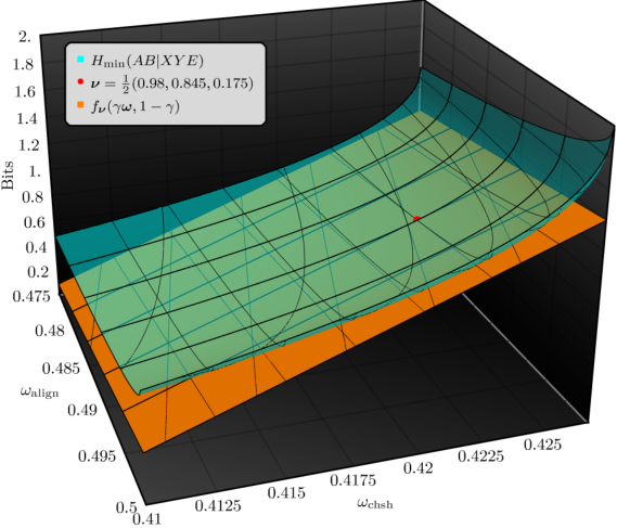
Taking the nonlocal game introduced in Example 2.1, we can use the above lemma to construct a min-tradeoff function. Fixing the probability of testing, , we consider a device that behaves (during a test round) according to the expected frequency distribution . In Fig. 3, we plot the certifiable min-entropy of a single generation round for a range of . We see that as the scores approach , we are able to certify almost1515 15 Due to the infrequent testing we are actually only able to certify a maximum of bits per interaction. two bits of randomness per entangled qubit pair using .
3.2 Accumulation and extraction
After fixing the parameters of the protocol and constructing a min-tradeoff function , the user proceeds with the remaining steps of Protocol QRE: accumulation and extraction. The accumulation step consists of the device interaction and evaluation sub-procedures that were detailed in Sec. 2.5.1. If the protocol does not abort, then with high probability the generated string contains at least some given quantity of smooth min-entropy. The following lemma applies the EAT to deduce a lower bound on the amount of entropy accumulated.
Lemma 3.3 (Accumulated entropy):
Let the randomness expansion procedure and all of its parameters be as defined in Fig. 2. Furthermore, let be the event the protocol does not abort (cf. (16)) and let be the final state of the system conditioned on this. Then, for any and any choice of min-tradeoff function , either Protocol QRE aborts with probability greater than or
| (33) |
where
| (34) |
| (35) |
| (36) |
and .
Proof.
Let be the set of channels implementing the entropy accumulation sub-procedure of Protocol QRE. Comparing this procedure with the definition of the EAT channels Def. 2.3, we have with finite dimensional classical systems, an arbitrary quantum system and the score is a deterministic function of the values of the other classical systems. Furthermore, the inputs to the protocol for the round, , are chosen independently of all other systems in the protocol and so the conditional independence constraints hold trivially. The conditions necessary for to be EAT-channels are satisfied and by Lemma 3.2 is a min-tradeoff function for these channels. We can now apply the EAT to bound the total entropy accumulated.
Consider now the pass probability of the protocol, . Either , in which case the protocol will abort with probability at least , or . In the latter case we can replace the unknown in (25) with as this results in an increase in the error term . The EAT then asserts that
for any choice of min-tradeoff function .
As the min-tradeoff functions are affine, we can lower bound the infimum for the region of possible scores specified by the success event,
Taking ), we have . Note that may not correspond to a frequency distribution that could have resulted from a successful run of the protocol – it may not even be a probability distribution. However, it is sufficient for our purposes as an explicit lower bound on the infimum. Further, noting that , we can straightforwardly compute this lower bound as
Inserting the min-tradeoff function properties (30)–(32) into the the EAT’s error terms [(23)–(25)] we get the explicit form of the quantities , and stated in the lemma. ∎
If the protocol does not abort during the accumulation procedure, the user may proceed by applying a quantum-proof strong extractor to the concatenated output string resulting in a close to uniform bit-string of length approximately .
Example 3.2:
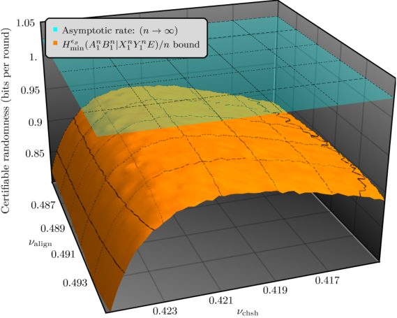
Continuing from Ex. 3.1, we look at the bound on the accumulated entropy specified by (33) for a range of choices of . Again, we are considering a quantum implementation with an expected frequency distribution . In Fig. 4 we see that our choice of min-tradeoff function can have a large impact on the quantity of entropy we are able to certify. The plot gives some reassuring numerical evidence that, for the nonlocal game , the certifiable randomness is continuous and concave in the family parameter .
The min-tradeoff function indexed by our expected frequency distribution, , is able to certify just under -bits per interaction. By applying a gradient-ascent algorithm we were able to improve this to -bits per interaction. In an attempt to avoid getting stuck within local optima we applied the algorithm several times, starting subsequent iterations at randomly chosen points close to the current optimum. The optimization led to an improved min-tradeoff function choice , where .
3.3 Protocol QRE
Protocol QRE is the concatenation of the accumulation and extraction sub-procedures. It remains to provide the formal security statements for a general instance of Protocol QRE. We refer to an untrusted device network as honest if during each interaction, the underlying quantum state shared amongst the devices and the measurements performed in response to inputs remain the same (i.e., the devices behave as the user expects). Furthermore, each interaction is performed independently of all others. The following lemma provides a bound on the probability that an honest implementation of Protocol QRE aborts.
Lemma 3.4 (Completeness of Protocol QRE):
Let Protocol QRE and all of its parameters be as defined in Fig. 2. Then, the probability that an honest implementation of Protocol QRE aborts is no greater than where
| (37) |
Proof.
During the parameter estimation step of Protocol QRE, the protocol aborts if the observed frequency distribution fails to satisfy
Writing , and , the probability that an honest implementation of the protocol aborts can be written as
Restricting to a single element of , we can model its final value as the binomially distributed random variable . As a consequence of the Chernoff bound (cf. Corollary B.1), and that , we have
Applying this bound to each element of the sum individually, we arrive at the desired result. ∎
Remark 3.1:
The completeness error in the above lemma only considers the possibility of the protocol aborting during the parameter estimation stage. However, if the initial random seed is a particularly limited resource then it is possible that the protocol aborts due to seed exhaustion. In Lemma B.4 we analyse a sampling algorithm required to select the inputs during device interaction. If required, the probability of failure for that algorithm could be incorporated into the completeness error.
With a secure bound on the quantity of accumulated entropy established by Lemma 3.3 we can apply a -strong extractor to to complete the security analysis. Combined with the input randomness discussed in Appendix B we arrive at the following theorem.
Lemma 3.5 (Soundness of Protocol QRE):
Let Protocol QRE be implemented with some initial random seed of length . Furthermore let all other protocol parameters be chosen within their permitted ranges, as detailed in Fig. 2. Then the soundness error of Protocol QRE is
Proof.
Recall from (13) that the soundness error is an upper bound on . In the case , we have .
Remark 3.2:
By choosing parameters such that we can take the soundness error to be .
Combining all of the previous results we arrive at the full security statement concerning Protocol QRE.
Theorem 3.1 (Security of Protocol QRE):
Remark 3.3:
The expected seed length required to execute Protocol QRE is (cf. Lemma B.4).
Example 3.3:
In Ex. 3.1 and Ex. 3.2 we used the following choice of protocol parameters: , , and . The resulting implementation of Protocol QRE, using the nonlocal game with an expected frequency distribution , exhibits the following statistics.
| Quantity | Value |
|---|---|
| Total accumulated entropy before extraction (no abort) | |
| Expected length of required seed before extraction | |
| Expected net-gain in entropy (no abort) | |
| Completeness error () |
4 Examples
In this section we demonstrate the use of our framework through the construction and analysis of several protocols based on different tests of nonlocality. To this end, we begin by introducing two families of nonlocal games which we consider alongside .
Empirical behaviour game . The empirical behaviour game is a nonlocal game that estimates the underlying behaviour of , i.e., it attempts to characterise each individual probability . We may construct this by associating with each input-output tuple a corresponding score and defining the scoring rule
for each . Then, for any input distribution with full support on the alphabets , the collection forms a nonlocal game. Moreover, for agents playing according to some strategy , the expected frequency distribution over the scores is precisely the joint distribution,
As can be defined for any collection of input-output alphabets, we can indicate the size of these alphabets as superscripts, i.e., . However, since we only consider binary output alphabets in this work, we will not include their sizes in the superscript, i.e., we will write instead of .
Remark 4.1:
The scoring rule for , as defined above, has several redundant components, arising from normalisation and the no-signalling conditions. In fact, there are only free parameters [51]. Knowing this we can reduce the number of scores in our nonlocal game and, in turn, the number of constraints we impose in our SDPs.1616 16 It is important to remove redundant constraints in practice as they can lead to numerical instabilities.
Joint correlators game . Specifically, for each we define a score and a scoring rule
That is, for a pair of inputs the score is recorded as whenever the agents’ outcomes agree. Otherwise, they record some normalization score . The input distribution can then be specified in some way: we use the uniform distribution over . We refer to this game by the symbol and, as before, we will indicate the sizes of the input alphabets with superscripts.
4.1 Rates in the presence of inefficient detectors
We now compare the accumulation rates of protocols built using the nonlocal games described above. We retain the protocol parameter choices from the previous examples: , and , except we now set the confidence interval width parameter to
| (39) |
in order to have a similar completeness error across the different protocols.1717 17 In practice one would fix the soundness error of the protocol. However, because the soundness error is also dependent on the extraction phase we instead assume independence of rounds and fix the completeness error.
We suppose that the devices operate by using a pure, entangled state of the form
| (40) |
for . We denote the corresponding density operator by . For simplicity we restrict to projective measurements within the - plane of the Bloch-sphere, i.e., measurements , with the projectors defined by
| (41) |
for . We denote the projectors associated with the outcome of the measurement by and . The elements of the devices’ behaviour can then be written as
| (42) |
Our analysis is focussed on how the accumulation rates differ when the devices operate with inefficient detectors. Heralding can be used to account for losses incurred during state transmission and has been used to develop novel device-independent protocols [52]. However, losses that occur within a user’s laboratory cannot be ignored without opening a detection loophole [53]. Inefficient detectors are a major contributor to the total experimental noise, so robustness to inefficient detectors is a necessary property for any practical randomness expansion protocol. We characterize detection efficiency by a single parameter , representing the (independent) probability with which a measurement device successfully measures a received state and outputs the result.1818 18 For simplicity, we make the additional assumption that the detection efficiencies are constant amongst all measurement devices used within the protocol. To deal with failed measurements we assign outcome when this occurs. Combining this with (42), we may write the behaviour as
| (43) | ||||
For each protocol we consider lower bounds on two quantities: the pre-EAT gain in min-entropy from a single interaction, , and the EAT-rate, . The former quantity, which we refer to as the asymptotic rate, represents the maximum accumulation rate achievable with our numerical technique. It is a lower bound on , specified by (33), as and , .1919 19 We would really like to plot and the corresponding EAT-rate derived from it. However, in general we do not have suitable techniques to access these quantities in a device-independent manner. Comparing these two quantities gives a clear picture of the amount of entropy that we lose due to the effect of finite statistics.
With inefficient detectors, partially entangled states can exhibit larger Bell-inequality violations than maximally entangled states [54]. To account for this we optimize both the state and measurement angles at each data point using the iterative optimization procedure detailed in [55]. All programs were relaxed to the second level of the NPA hierarchy using [56] and the resulting SDPs were computed using the SDPA solver [57]. The results of these numerics are displayed in Fig. 5.
In Fig. 5(a) and Fig. 5(b) we see that in both families of protocols considered, an increase in the number of inputs leads to higher rates. This increase is significant when one moves from the -scenario to the -scenario. However, continuing this analysis for higher numbers of inputs we find that any further increases appear to have negligible impact on the overall robustness of the protocol.2020 20 This could also be an artefact of the assumed restriction to qubit systems. Whilst all of the protocols achieve asymptotic rates of bits per round when , their respective EAT-rates at this point differ substantially. In Fig. 5(c) we see a direct comparison between protocols from the different families. The plot shows that, as expected, entropy loss is greater when using the nonlocality test as opposed to the other protocols. In particular, for high values of we find that we would be able to certify a larger quantity of entropy by considering fewer scores. However, it is still worth noting that this entropy loss could be reduced by choosing a more generous set of protocol parameters, e.g., increasing and decreasing .
Increasing can be difficult in practice due to restrictions on the overall runtime of the protocol. Not only does it take longer to collect the statistics within the device-interaction phase, but it may also increase the runtime of the extraction phase [58]. In Fig. 6 we observe how quickly the various protocols converge on their respective asymptotic rates as we increase . Again we find that, due to the finite-size effect, entropy loss when using is greater than that observed in the other protocols. In particular, we see that for protocols with fewer than rounds, it is advantageous to use . From the perspective of practical implementation, Fig. 5(c) and Fig. 6 highlight the benefits of a flexible protocol framework wherein a user can design protocols tailored to the scenario under consideration.
It is also important to compare the rates of instances of Protocol QRE with other protocols from the literature, in particular the protocol of [14] (ARV). In [14], the min-tradeoff functions are constructed from a tight bound on the single-party von Neumann entropy, , which is given in terms of a CHSH inequality violation [35]. In Fig. 7 we compare the rates of ARV with and for entangled qubit systems with inefficient detectors. To make our comparison fair, we have also computed the rates for Protocol ARV using the improved EAT bound2121 21 Note that we always use the direct bound on the von Neumann entropy when considering Protocol ARV, rather than forming a bound via the min-entropy. As the rates of Protocol ARV are derived from the entropy accumulated by a single party their rates are capped at one bit per round.
In contrast, the semidefinite programs grant us access to bounds on the entropy produced by both parties and we are therefore able to certify up to two bits per round. In Fig. 7, this advantage is observed in the high detection efficiency regime. Fig. 7 also highlights a significant drawback of our technique, which stems from our use of the inequality . In particular, we see that for , the bound for the CHSH inequality is already greater than the established for the empirical behaviour. Therefore, in the asymptotic limit () the min-entropy bounds for these protocols will produce strictly worse rates in this regime. For the finite we have chosen, , it appears that for the majority of smaller , it is advantageous to use the ARV protocol over the protocols derived from the framework. Nevertheless, looking at the threshold detection efficiencies, i.e. the minimal detection efficiency required to achieve positive rates, we find that some protocols from our framework are able to again beat the rates established for Protocol ARV. Looking at the inset plot in Fig. 7 we see that has a smaller threshold efficiency than that of Protocol ARV for the chosen protocol parameters. Interestingly, this shows that is capable of producing higher rates than Protocol ARV in both the low and the high detection efficiency regimes, with the improvement for low detection efficiencies being of particular relevance to experimental implementations. Importantly, this shows that protocols from the framework are of practical use for finite in spite of the losses coming from the use of .
Remark 4.2:
We have so far considered the only noise to be that caused by inefficient detectors. However, it is natural to ask how other sources of noise affect our results. By replacing the states used with Werner states [59], we find that the results remain robust—they remain qualitatively the same, but for small Werner state noise, all of the graphs shift to slightly lower rates. For this reason we choose not to include the graphs here.
5 Conclusion
We have shown how to combine device-independent bounds on the guessing probability with the EAT, to create a versatile method for analysing quantum-secure randomness expansion protocols. The construction was presented as a template protocol from which an exact protocol can be specified by the user. The relevant security statements and quantity of output randomness of the derived protocol can then be evaluated numerically. A Python package [24] accompanies this work to help facilitate implementation of the framework. In Sec. 4 we illustrated the framework, applying it to several example protocols, with parameters chosen to reflect the capabilities of current nonlocality tests. We then compared the robustness of these protocols when implemented on qubit systems with inefficient detectors. Our analyses show that, within a broadly similar experimental setup, different protocols can have significantly different rates, and hence that it is worth considering small modifications to a protocol during their design. We also compared the rates of a selection of our protocols to the protocol presented in [14] (ARV). Interestingly, we found that some of the protocols from the framework are able to achieve higher rates than Protocol ARV in both the high and low detection efficiency regimes. In particular, the higher rates for low detection efficiencies is of great importance for actual experimental implementations.
Although the framework produces secure and robust protocols, there remains scope for further improvements. For example, our work relies on the relation which is far from tight. The resulting loss can be seen when one compares the asymptotic rate of in Fig. 5(c) with those presented in [14] (see Fig. 7). Several alternative approaches could be taken in order to reduce this loss. Firstly, the above relation is part of a more general ordering of the conditional Rényi entropies.2222 22 The Rényi entropies are one of many different entropic families that include the von Neumann entropy as a limiting case. Any such family could be used if they satisfy an equivalent relation. If one were able to develop efficient computational techniques for computing device-independent lower bounds on one of these alternative quantities we would expect an immediate improvement. Furthermore, dimension-dependent bounds may be applicable in certain situations. For example, it is known that for the special case of -party, -input, -output scenarios it is sufficient to restrict to qubit systems [51, 35].
Optimizing the choice of min-tradeoff function over is a non-convex and not necessarily continuous problem [60]. Our analysis in Sec. 4 used a simple probabilistic gradient ascent algorithm to approach this problem. We found that for certain protocols, in particular , the optimization had to be repeated many times before a good choice of min-tradeoff function was found.
As Fig. 7 shows, the framework is capable of producing protocols that are of immediate relevance to current randomness expansion experiments. It is therefore a worthwhile endeavour to search for protocols within the framework that provide high EAT-rates in different parameter regimes. Investigations into the randomness certification properties of nonlocality tests with larger output alphabets or additional parties could be of interest. However, increasing either of these parameters is likely to increase the influence of finite-size effects. Alternatively, one could try to design more economical nonlocality tests by combining scores that are of a lesser importance to the task of certifying randomness. Intuitively, for a score , the magnitude of of in the min-tradeoff function indicates how important that score is for certifying entropy. If is large then this score is ‘important’ in the sense that any small deviations in the expected frequency of that score, , will have a large impact on the amount of certifiable entropy. Another approach to designing good nonlocality tests would be to take inspiration from [20, 21] wherein the authors showed how to derive the optimal Bell-expressions for certifying randomness. A nonlocal game could then be designed to encode the constraints imposed by this optimal Bell-expression. An example of such a game would be to assign a score to all that have a positive coefficient in the optimal Bell-expression and a score of to all those with negative coefficients. The input distribution of the nonlocal game could then be chosen as such to encode the relative weights of the coefficients.
Finally, our computational approach to the EAT considered only the task of randomness expansion. Our work could be extended to produce security proofs for other device-independent tasks. Given that the EAT has already been successfully applied to a wide range of problems [62, 63, 36, 64, 65], developing good methods for robust min-tradeoff function constructions represents an important step towards practical device-independent security.
Acknowledgments
We are grateful for support from the EPSRC’s Quantum Communications Hub (grant number EP/M013472/1), an EPSRC First Grant (grant number EP/P016588/1) and the WW Smith fund.
References
- [1] N. Heninger, Z. Durumeric, E. Wustrow, and J. A. Halderman, “Mining your Ps and Qs: Detection of widespread weak keys in network devices,” in Proceedings of the 21st USENIX Security Symposium, Aug. 2012.
- [2] P. Chaiwongkhot, S. Sajeed, L. Lydersen, and V. Makarov, “Finite-key-size effect in a commercial plug-and-play QKD system,” Quantum Science and Technology, vol. 2, no. 4, p. 044003, 2017.
- [3] D. Mayers and A. Yao, “Quantum cryptography with imperfect apparatus,” in Proceedings of the 39th Annual Symposium on Foundations of Computer Science (FOCS-98), (Los Alamitos, CA, USA), pp. 503–509, IEEE Computer Society, 1998.
- [4] A. K. Ekert, “Quantum cryptography based on Bell’s theorem,” Physical Review Letters, vol. 67, no. 6, pp. 661–663, 1991.
- [5] R. Colbeck, Quantum and Relativistic Protocols For Secure Multi-Party Computation. PhD thesis, University of Cambridge, 2007. Also available as arXiv:0911.3814.
- [6] R. Colbeck and A. Kent, “Private randomness expansion with untrusted devices,” Journal of Physics A, vol. 44, no. 9, p. 095305, 2011.
- [7] S. Pironio, A. Acin, S. Massar, A. Boyer de la Giroday, D. N. Matsukevich, P. Maunz, S. Olmschenk, D. Hayes, L. Luo, T. A. Manning, and C. Monroe, “Random numbers certified by Bell’s theorem,” Nature, vol. 464, pp. 1021–1024, 2010.
- [8] S. Pironio and S. Massar, “Security of practical private randomness generation,” Physical Review A, vol. 87, p. 012336, 2013.
- [9] S. Fehr, R. Gelles, and C. Schaffner, “Security and composability of randomness expansion from Bell inequalities,” Physical Review A, vol. 87, p. 012335, 2013.
- [10] C. A. Miller and Y. Shi, “Universal security for randomness expansion from the spot-checking protocol,” arXiv preprint arXiv:1411.6608, 2014.
- [11] C. A. Miller and Y. Shi, “Robust protocols for securely expanding randomness and distributing keys using untrusted quantum devices,” in Proceedings of the 46th Annual ACM Symposium on Theory of Computing, STOC ’14, (New York, NY, USA), pp. 417–426, ACM, 2014.
- [12] U. Vazirani and T. Vidick, “Certifiable quantum dice or, testable exponential randomness expansion,” in Proceedings of the 44th Annual ACM Symposium on Theory of Computing (STOC-12), pp. 61–76, 2012.
- [13] F. Dupuis, O. Fawzi, and R. Renner, “Entropy accumulation.” e-print arXiv:1607.01796, 2016.
- [14] R. Arnon-Friedman, R. Renner, and T. Vidick, “Simple and tight device-independent security proofs.” SIAM Journal on Computing, vol. 48, no. 1, pp. 181–225, 2019.
- [15] R. Arnon-Friedman, F. Dupuis, O. Fawzi, R. Renner, and T. Vidick, “Practical device-independent quantum cryptography via entropy accumulation,” Nature communications, vol. 9, no. 1, p. 459, 2018.
- [16] E. Knill, Y. Zhang, and H. Fu, “Quantum probability estimation for randomness with quantum side information.” e-print arXiv:1806.04553, 2018.
- [17] O. Nieto-Silleras, C. Bamps, J. Silman, and S. Pironio, “Device-independent randomness generation from several Bell estimators,” New Journal of Physics, vol. 20, no. 2, p. 023049, 2018.
- [18] M. Navascués, S. Pironio, and A. Acín, “Bounding the set of quantum correlations,” Physical Review Letters, vol. 98, no. 1, p. 010401, 2007.
- [19] M. Navascués, S. Pironio, and A. Acín, “A convergent hierarchy of semidefinite programs characterizing the set of quantum correlations,” New Journal of Physics, vol. 10, no. 7, p. 073013, 2008.
- [20] O. Nieto-Silleras, S. Pironio, and J. Silman, “Using complete measurement statistics for optimal device-independent randomness evaluation,” New Journal of Physics, vol. 16, no. 1, p. 013035, 2014.
- [21] J.-D. Bancal, L. Sheridan, and V. Scarani, “More randomness from the same data,” New Journal of Physics, vol. 16, no. 3, p. 033011, 2014.
- [22] R. König, R. Renner, and C. Schaffner, “The operational meaning of min- and max-entropy,” IEEE Transactions on Information Theory, vol. 55, no. 9, pp. 4337–4347, 2009.
- [23] F. Dupuis and O. Fawzi, “Entropy accumulation with improved second-order,” IEEE Transactions on information theory, 2019.
- [24] “Python package for DI protocol development.” https://github.com/peterjbrown519/dirng, 2018.
- [25] P. Mironowicz and M. Pawowski. “Robustness of quantum-randomness expansion protocols in the presence of noise,” Physical Review A vol. 88.3, p. 032319, 2013.
- [26] M. Giustina, M. A. M. Versteegh, S. Wengerowsky, J. Handsteiner, A. Hochrainer, K. Phelan, F. Steinlechner, J. Kofler, J.-A. Larsson, C. Abellan, W. Amaya, V. Pruneri, M. W. Mitchell, J. Beyer, T. Gerrits, A. E. Lita, L. K. Shalm, S. W. Nam, T. Scheidl, R. Ursin, B. Wittmann, and A. Zeilinger, “Significant-loophole-free test of Bell’s theorem with entangled photons,” Physical Review Letters vol. 115, p. 250401, 2015.
- [27] L. K. Shalm, E. Meyer-Scott, B. G. Christensen, P. Bierhorst, M. A. Wayne, M. J. Stevens, T. Gerrits, S. Glancy, D. R. Hamel, M. S. Allman, K. J. Coakley, S. D. Dyer, C. Hodge, A. E. Lita, V. B. Verma, C. Lambrocco, E. Tortorici, A. L. Migdall, Y. Zhang, D. R. Kumor, W. H. Farr, F. Marsili, M. D. Shaw, J. A. Stern, C. Abellan, W. Amaya, V. Pruneri, T. Jennewein, M. W. Mitchell, P. G. Kwiat, J. C. Bienfang, R. P. Mirin, E. Knill, and S. W. Nam, “Strong loophole-free test of local realism,” Physical Review Letters vol. 115, p. 250402, 2015.
- [28] B. Hensen, H. Bernien, A. E. Dréau, A. Reiserer, N. Kalb, M. S. Blok, J. Ruitenberg, R. F. L. Vermeulen, R. N. Schouten, C. Abella, W. Amaya, V. Pruneri, M. W. Mitchell, M. Markham, D. J. Twitchen, D. Elkouss, S. Wehner, T. H. Taminiau, and R. Hanson, “Loophole-free Bell inequality violation using electron spins separated by 1.3 kilometres,” Nature vol. 526, pp. 682–686, 2015.
- [29] G. Murta, S. B. van Dam, J. Ribeiro, R. Hanson, and S. Wehner, “Towards a realization of device-independent quantum key distribution,” arXiv preprint arXiv:1811.07983, 2018.
- [30] R. Renner, Security of Quantum Key Distribution. PhD thesis, Swiss Federal Institute of Technology, Zurich, 2005. Also available as quant-ph/0512258.
- [31] R. Renner and S. Wolf, “Smooth Rényi entropy and applications,” in Information Theory, 2004. ISIT 2004. Proceedings. International Symposium on, p. 233, IEEE, 2004.
- [32] M. Tomamichel, R. Colbeck, and R. Renner, “Duality between smooth min- and max-entropies,” IEEE Transactions on information theory, vol. 56, no. 9, pp. 4674–4681, 2010.
- [33] M. Tomamichel, Quantum Information Processing with Finite Resources: Mathematical Foundations, vol. 5. Springer, 2015.
- [34] E. Hänggi and R. Renner, “Device-independent quantum key distribution with commuting measurements.” e-print arXiv:1009.1833, 2010.
- [35] A. Acin, N. Brunner, N. Gisin, S. Massar, S. Pironio, and V. Scarani, “Device-independent security of quantum cryptography against collective attacks,” Physical Review Letters, vol. 98, p. 230501, 2007.
- [36] M. Kessler and R. Arnon-Friedman, “Device-independent randomness amplification and privatization,” arXiv preprint arXiv:1705.04148, 2017.
- [37] N. Brunner, D. Cavalcanti, S. Pironio, V. Scarani, and S. Wehner, “Bell nonlocality,” Reviews of Modern Physics, vol. 86, no. 2, p. 419, 2014.
- [38] S. Popescu and D. Rohrlich, “Which states violate Bell’s inequality maximally?,” Physics Letters A, vol. 169, no. 6, pp. 411–414, 1992.
- [39] R. Canetti, “Security and composition of multiparty cryptographic protocols,” Journal of Cryptology, vol. 13, no. 1, pp. 143–202, 2000.
- [40] R. Canetti, “Universally composable security: A new paradigm for cryptographic protocols.,” in Proceedings of the 42nd Annual Symposium on Foundations of Computer Science (FOCS-01), pp. 136–145, 2001.
- [41] B. Pfitzmann and M. Waidner, “A model for asynchronous reactive systems and its application to secure message transmission,” in Proceedings of the 2001 IEEE Symposium on Security and Privacy (SP01), (Washington, DC, USA), pp. 184–201, IEEE Computer Society, 2001.
- [42] M. Ben-Or and D. Mayers, “General security definition and composability for quantum & classical protocols.” e-print quant-ph/0409062, 2004.
- [43] C. Portmann and R. Renner, “Cryptographic security of quantum key distribution,” arXiv preprint arXiv:1409.3525, 2014.
- [44] J. Barrett, R. Colbeck, and A. Kent, “Memory attacks on device-independent quantum cryptography,” Physical Review Letters, vol. 106, p. 010503, 2013.
- [45] M. Tomamichel, R. Colbeck, and R. Renner, “A fully quantum asymptotic equipartition property,” IEEE Transactions on information theory, vol. 55, no. 12, pp. 5840–5847, 2009.
- [46] M. Ledoux, The concentration of measure phenomenon. American Mathematical Soc., 2005.
- [47] A. De, C. Portmann, T. Vidick, and R. Renner, “Trevisan’s extractor in the presence of quantum side information.” e-print arXiv:0912.5514, 2009.
- [48] R. Konig and R. Renner, “Sampling of min-entropy relative to quantum knowledge,” IEEE Transactions on Information Theory, vol. 57, no. 7, pp. 4760–4787, 2011.
- [49] L. Trevisan, “Extractors and pseudorandom generators,” Journal of the ACM, vol. 48, no. 4, pp. 860–879, 2001.
- [50] N. Nisan and A. Ta-Shma, “Extracting randomness: A survey and new constructions,” J. Comput. Syst. Sci., vol. 58, no. 1, pp. 148–173, 1999.
- [51] B. Tsirelson, “Some results and problems on quantum Bell-type inequalities,” Hadronic Journal Supplement, vol. 8, pp. 329–345, 1993.
- [52] A. Máttar, J. Kolodyński, P. Skrzypczyk, D. Cavalcanti, K. Banaszek, and A. Acín, “Device-independent quantum key distribution with single-photon sources,” arXiv preprint arXiv:1803.07089, 2018.
- [53] P. M. Pearle, “Hidden-variable example based upon data rejection,” Physical Review D, vol. 2, no. 8, pp. 1418–1425, 1970.
- [54] P. H. Eberhard, “Background level and counter efficiencies required for a loophole-free Einstein-Podolsky-Rosen experiment,” Physical Review A, vol. 47, pp. 747–750, 1993.
- [55] S. M. Assad, O. Thearle, and P. K. Lam, “Maximizing device-independent randomness from a Bell experiment by optimizing the measurement settings,” Physical Review A, vol. 94, no. 1, p. 012304, 2016.
- [56] P. Wittek, “Algorithm 950: Ncpol2sdpa - sparse semidefinite programming relaxations for polynomial optimization problems of noncommuting variables,” ACM Transactions on Mathematical Software (TOMS), vol. 41, no. 3, p. 21, 2015.
- [57] K. Fujisawa, M. Kojima, K. Nakata, and M. Yamashita, “SDPA (semidefinite programming algorithm) user’s manual -— version 6.2.0,” Department of Mathematical and Com-puting Sciences, Tokyo Institute of Technology. Research Reports on Mathematical and Computing Sciences Series B: Operations Research, 2002.
- [58] W. Mauerer, C. Portmann, and V. B. Scholz, “A modular framework for randomness extraction based on Trevisan’s construction,” arXiv preprint arXiv:1212.0520, 2012.
- [59] R. Werner, “Quantum states with Einstein-Podolsky-Rosen correlations admitting a hidden-variable model,” Physical Review A, vol. 40, no. 8, p. 4277, 1989.
- [60] F. J. Curchod, M. Johansson, R. Augusiak, M. J. Hoban, P. Wittek, and A. Acín, “Unbounded randomness certification using sequences of measurements,” Physical Review A, vol. 95, no. 2, p. 020102, 2017.
- [61] A. Acín, S. Massar, and S. Pironio, “Randomness versus nonlocality and entanglement,” Phys. Rev. Lett., vol. 108, p. 100402, Mar 2012.
- [62] J. Ribeiro, G. Murta, and S. Wehner, “Fully device-independent conference key agreement,” Phys. Rev. A, vol. 97, p. 022307, Feb 2018.
- [63] J. Ribeiro, L. P. Thinh, J. Kaniewski, J. Helsen, and S. Wehner, “Device independence for two-party cryptography and position verification with memoryless devices,” Phys. Rev. A, vol. 97, p. 062307, Jun 2018.
- [64] R. Arnon-Friedman and J.-D. Bancal, “Device-independent certification of one-shot distillable entanglement,” arXiv preprint arXiv:1712.09369, 2017.
- [65] C. Bamps, S. Massar, and S. Pironio, “Device-independent randomness generation with sublinear shared quantum resources,” Quantum, vol. 2, p. 86, 2018.
- [66] H. Chernoff, “A measure of asymptotic efficiency for tests of a hypothesis based on the sum of observations,” The Annals of Mathematical Statistics, vol. 23, no. 4, pp. 493–507, 1952.
- [67] T. Hagerup and C. Rüb, “A guided tour of Chernoff bounds,” Information Processing Letters, vol. 33, pp. 305–308, 1990.
- [68] W. Hoeffding, “Probability inequalities for sums of bounded random variables,” Journal of the American Statistical Association, vol. 58, no. 301, pp. 13–30, 1963.
- [69] T. S. Han and M. Hoshi, “Interval algorithm for random number generation,” IEEE Transactions on Information Theory, vol. 43, no. 2, pp. 599–611, 1997.
- [70] T. M. Cover and J. A. Thomas, Elements of Information Theory. John Wiley and Sons Inc., 2nd ed., 2006.
- [71] S. Boyd and L. Vandenberghe, Convex optimization. Cambridge University Press, 2004.
Appendix A Table of parameters and notation
| Notation | Description | Initial reference |
| A collection of untrusted devices. | Section 2.3 | |
| A nonlocal game. | Definition 2.1 | |
| Set of expected frequency distributions on using quantum strategies. | Section 2.3 | |
| Set of expected frequency distributions on using strategies from . | Section 2.3 | |
| Expected frequency distributions over scores of a nonlocal game. | Equation 11 | |
| , | Solutions to the -relaxed primal and dual guessing probability programs. | Program 9 and 10 |
| Feasible point of the dual guessing probability program with parameter . | Section 2.3 | |
| Vector of statistical confidence interval widths. | Equation 16. | |
| with elements signed in accordance with a given . | Lemma 3.3 | |
| Devices’ output alphabets. | Section 2.1 | |
| Devices’ input alphabets. | Section 2.1 | |
| Number of rounds in the device-interaction phase. | Section 2.5.1 | |
| Probability that any given round is a test round. | Section 2.5.1 | |
| Devices’ outputs for the round. | Section 2.5.1 | |
| Devices’ inputs for the round. | Section 2.5.1 | |
| EAT-score for the round. | Section 2.5.1 | |
| Frequency distribution induced by score transcript . | Equation 15 | |
| Event that the protocol does not abort. | Equation 16 | |
| Strong quantum-secure randomness extractor. | Definition 2.5 | |
| Completeness error of Protocol QRE. | Lemma 3.4 | |
| Soundness error of Protocol QRE. | Lemma 3.5 | |
| Smoothing parameter for . | Equation 7 | |
| Tolerance of unlikely success events. | Lemma 3.3. | |
| EAT error term (Variance). | Theorem 2.1 | |
| EAT error term (Remainder). | Theorem 2.1 | |
| EAT error term (Pass probability). | Theorem 2.1 | |
| Extractor error. | Definition 2.5 | |
| Entropy lost during extraction. | Section 2.6 |
Appendix B Input Randomness
Here we quantify the length of the initial random seed required to execute an instance of Protocol QRE. This supply of random bits is necessary for selecting the devices’ inputs and seeding the extractor. In the forthcoming analysis we ignore the latter as this quantity depends on the choice of extractor. Instead, we look at the process of converting a uniform private seed into device inputs required for running Protocol QRE. We follow a similar procedure to that used in [14], modifying the algorithm slightly in order to extract explicit bounds.
B.1 Statistical bounds
We begin by stating some standard statistical bounds. The first is commonly known as the Chernoff bound [66], although we take our formulation from [67]. This provides a convenient bound on the deviation of the sum of random variables from the expected value.
Lemma B.1 (Chernoff bound):
Let be independent binary random variables for , and . Then for
Corollary B.1:
For we have .
In addition to this, we also make use of Hoeffding’s inequality [68].
Lemma B.2 (Hoeffding’s inequality):
Let be independent random variables, such that with for . In addition, let and . Then for
B.2 Rounded interval algorithm
The interval algorithm provides an efficient method for simulating the sampling of some target random variable using another random variable . To aid understanding of our modification to this algorithm and any subsequent results we shall briefly explain how this simulation works. For simplicity we restrict ourselves to the scenario where is a sequence of uniformly distributed bits, we denote the uniform distribution on an alphabet of size by , for .
The distribution of the target random variable forms a partition of the unit interval, one subinterval for each outcome of . In exactly the same way, the probability distribution for partitions the unit interval into subintervals. Thus, we can associate a bit-string with its corresponding subinterval, defined by this partitioning. The interval algorithm works by using an increasing sequence of random bits and the corresponding subintervals that the sequence defines. Once the subinterval generated by the sequence of bits is contained inside one of the subintervals defined by the target random variable , say , then we say that we have simulated the sampling of from and the algorithm terminates. Denoting by the length of seed required for the interval algorithm to terminate, then by [69, Theorem 3] we have
| (44) |
As the algorithm stands, the maximum value that can take is unbounded (although the probability that the algorithm expends the seed without terminating decreases exponentially in ). In order to produce large deviation bounds on the number of bits required to execute our protocol, we place an upper limit on the maximum seed length. We thus use an adapted sampling procedure, the rounded interval algorithm (RIA), which forcefully terminates if the seed length reaches the upper bound of bits.
Should the RIA fail to terminate after steps, then the output sequence generated will correspond to some subinterval , for some , that is not entirely contained within one of the subintervals induced by . If this occurs, we round down: selecting the interval for which .
Remark B.1:
Note that the above procedure depends on the ordering of the intervals generated by (which should be fixed before sampling). One could imagine a rather pathological scenario where an ordering places extremely unlikely outcomes over rounding points, greatly increasing their simulated outcome probabilities. However, as will be shown in Lemma B.3, the distance between the simulated random variable and the target random variable decreases exponentially in .
Remark B.2:
The rounding procedure truncates the maximum seed length, , and as such, it is clear that the inequality (44) also holds for the RIA.
Definition B.1 (Statistical distance):
Given two random variables and , taking values in some common alphabet . The statistical distance between and , is defined by
| (45) |
Lemma B.3:
Let be a random variable taking values in some alphabet . Let be the distribution sampled using the RIA with target distribution . Then
where is the maximum number of input bits that can be used by the RIA.
Proof.
Consider the partitions of the unit interval and corresponding to the distributions and of and respectively. The intervals of take the form
where the (potentially empty) union is taken over all such that . The intervals within the union are either contained fully within the corresponding outcome interval of , i.e., , or they are included as a result of rounding. Thus we may write
By a straightforward counting argument, there are at least such values of , and at most . We hence have
and therefore
holds for all . Applying this bound to each term within the sum completes the proof. ∎
B.3 Input randomness for Protocol QRE
Following the structure of Protocol QRE, we look to use the RIA to sample the devices’ inputs for each round. In adherence with the Markov-chain condition (Def. 2.3), the natural procedure would be to sample at the beginning of each round. However, in practice this requires a much larger seed: because of (44) and the property , by sampling the joint distribution the expected saving is about bits compared to repeating a single sample times. Fortunately, this joint sampling can be implemented while maintaining the Markov-chain condition. Within the assumptions of Protocol QRE we allow the honest parties access to a trusted classical computer, which would also contain some trusted data storage—we assume that the parties can record their outcome strings without leakage. Therefore, using their trusted classical computer, the honest parties perform the RIA: sampling the random variables and subsequently storing the outcome on the trusted classical computer’s harddrive. Crucially, the assumption that the user can prevent unwanted communication between devices implies this can all be done without any information leaking to the untrusted devices. Then, at the beginning of round , the inputs are sent from the classical computer to the respective devices. By conducting the protocol in this manner we retain the Markov chain conditions—the inputs are sampled independently of the devices and furthermore, when the devices produce their outputs for the round they can only have knowledge of the inputs for this round and all previous.
Due to potential computational constraints and to permit large deviation bounds on the number of bits required we will not assume that all rounds are sampled at once. Instead, we split the rounds into at most blocks of size and apply the RIA to sample the inputs of each block separately. For simplicity, we assume that and henceforth remove the ceiling function from the analysis.
Recall that for the round, the user first uses to decide whether the round is a test round, and, if so, they choose inputs according to the nonlocal game input distribution . Otherwise, if , they supply their devices with the fixed inputs and . The probability mass function of joint random variables , representing the round’s inputs, is therefore
| (46) |
Following (44), if is the seed length required to sample one of the blocks of rounds, then we have
| (47) |
where is the Shannon entropy of the distribution and is the binary entropy.
The following lemma gives a probabilistic bound on the total length of the random seed required to sample the inputs for the devices.2323 23 We do not include the extractor’s seed here as its size will depend on the choice of extractor.
Lemma B.4:
Let the parameters of Protocol QRE be as defined in Fig. 2 and let be the maximum permitted seed length for an instance of the RIA. Then, with probability greater than , we can use instances of the RIA to simulate the sampling of every device input required to execute Protocol QRE with a uniform seed of length no greater than , where
| (48) | ||||
| (49) | ||||
| and . Moreover, the sampled distribution lies within a statistical distance of | ||||
| (50) | ||||
from the target distribution, where .
Proof.
Consider the sequence of i.i.d. random variables representing the number of random bits required to choose the inputs for the block and the corresponding random sum . By (47), the expected number of bits required to select all of the inputs for the protocol can be bounded above by . Using Hoeffding’s inequality, we can bound the probability that greatly exceeds this value,
for some . Setting this becomes
Although is not exactly the expected value of , which is the quantity appearing in Hoeffding’s bound, the bound holds because .
It remains to bound the statistical distance between the sampled random variable and the target random variable . For each block of rounds, the corresponding random variable can take one of a possible different values. Therefore, by Lemma B.3, we have for the block of rounds
Since is a metric and hence satisfies the triangle inequality [70], the statistical distance between independently repeated samples can grow no faster than linearly, i.e., . This completes the proof. ∎
Appendix C Incorporating the blocking procedure of [14]
The original statement of the entropy accumulation theorem [13] was released alongside an accompanying paper, [14], which detailed its application to security proofs of device-independent protocols. Within the appendix of [14] it was shown that one could increase the quantity of entropy certified by the original EAT by modifying the structure of the protocol. In particular, this demonstrated the original EAT statement’s suboptimal dependence on the testing probability. In light of this, the authors of [23] improved the second order term of the EAT in order to account for this suboptimal dependence. In the sections that follow, we will look at how the modified protocol structure interacts with the improved EAT statement. We begin by showing how the family of min-tradeoff functions can be adapted to this structural change and then we show that the modified protocol structure provides no clear benefits when used with the improved EAT statement. In addition, we provide some comparison plots showing the accumulation rates achievable with the different structures and EAT statements. To clearly distinguish the different statements of the EAT, we shall indicate with the subscript , quantities associated with the original EAT [13] and similarly we shall indicate with the subscript , quantities associated with the EAT with improved second-order [23].
C.1 Construction
Let us briefly review the structural modification that was introduced in [14]. Instead of distinguishing the statistics from each interaction separately, rounds are grouped together to form blocks. The number of rounds within a block can vary: a new block begins when either a test-round occurs or when the maximum number of rounds permitted within a block, , is reached. On expectation there are rounds within a block. The device-interaction phase of the protocol concludes after some specified number of blocks have terminated. We shall use the superscripts and to indicate whether a quantity is concerned with the round-by-round or block structured protocols respectively.
The collected information is now defined at the level of blocks and not rounds. In particular, at the end of the block the user records some tuple , where and the score’s alphabet remains the same, . The EAT-channels are also defined for each block and the entropy bounding property (cf. (17)) that the min-tradeoff functions must satisfy becomes
| (51) |
for each . The set of distributions compatible with the protocol structure (cf. (18)) now take the form
| (52) |
for .
Lemma C.1 (Blocked variant of Lemma 3.1):
Let be an affine function satisfying
| (53) |
for all . Then the function , defined by its action on trivial distributions
is a min-tradeoff function for any EAT-channels implementing Protocol QREB. Furthermore, satisfies the following properties:
Proof.
This follows from replicating the original proof [23] with the block channels decomposed into the testing and generation channels, . ∎
Lemma C.2 (Blocked min-tradeoff construction):
Let be a nonlocal game and . For each , let be some feasible point of Prog. (10). Furthermore, let and . Then, for any set of EAT channels implementing an instance of Protocol QREB with the nonlocal game , the set of functionals forms a family of min-tradeoff functions, where are defined by their actions on trivial distributions
| (54) | ||||
| and | ||||
| (55) | ||||
where and .
Moreover, these min-tradeoff functions satisfy the following identities.
- •
Maximum:
(56) - •
-Minimum:
(57) - •
-Variance:
(58)
Proof.
The proof follows the same structure as the proof of Lemma 3.2. The only significant difference is the construction of the function satisfying (53) so we shall explain this part here. Following Appendix B of [14], by repeated application of the chain rule we may decompose a block’s entropy as
where is the random variable indicating whether a test occurred on the round of the block. Considering the individual terms within the sum, we can absorb the majority of the side information into some arbitrary quantum register leaving us with terms of the form
As before, we can use the inequality and conditioning on to lower bound each term in the sum by the outputs of the semidefinite program,
where is the expected frequency distribution over the games scores for round of block . Noting that of a linear function is convex, we can establish a bound on the entire block through an application of Jensen’s inequality
we have used the fact that and that is the normalised expected frequency distribution over the nonlocal game scores for the block. Taking a first-order expansion of the last line, we get the function . The proof is then completed by applying the extension Lemma C.1, analogous to the technique of Lemma 3.2. ∎
C.2 Blocking with the improved second order
The error term in the original EAT bound is
| (59) |
The disadvantage of using this bound as-is is that the gradient of scales like and so the total error scales as . Collating the statistics into blocks, allows some of the dependence from the gradient term to be transferred to the term. Moving to the blocked structure and setting (as was done in [14]), the output alphabets grow exponentially with the size of the block and the logarithmic term acquires a scaling. In contrast, the scaling of the derivative of the min-tradeoff function is found to be independent of the block size. Fortunately, as our error is defined for an entire block, we reduce the multiplicative factor on the total error from to . As , we find that the total error term now scales as . By increasing the size of the blocks we have effectively redistributed the testing probability dependence evenly amongst the components of .
In [23], the authors looked to amend this deficiency by strengthening the second order term in the EAT. The following short calculation looks at how the errors scale when we applying the blocking procedure to the improved EAT statement. Recall the error terms
| (60) |
| (61) |
and
| (62) |
Using the explicit form of the blocked min-tradeoff functions Lemma C.2, we can calculate the asymptotic growth of the error terms as , and . In particular, we find
| (63) | ||||
| (64) | ||||
| (65) |
and therefore the total error scales as
| (66) |
In order for to have any sensible scaling, we need the exponent to grow no faster than . Combining this with the inverse dependence of in , we would like . Such a choice results in which suggests that indeed, the blocking procedure is no longer advantageous when used in conjunction with the improved second order statement.
A comparison between the expansion rates obtained when using the improved second order statement [23] and the blocked variant of the original EAT are presented in Fig. 8. The faster convergence to the asymptotic rate is indicative of the new EAT statement’s strength.
Appendix D Conic program duality
In this section we outline the duality statements for conic programs, introduce the alternative form of dual that we use in this paper and show that it has the required properties to be considered a dual.
Definition D.1:
A cone is a set with the property that if then for all . A cone is pointed if .
Definition D.2:
Given a cone , its dual cone is the set defined by the property that if and only if for all , i.e., .
Definition D.3:
A proper cone is a cone that is closed, convex, pointed and non-empty.
Definition D.4 (Dual for conic programs):
Let be a proper cone with dual , , and consider the conic program
The optimization
is the dual program.
Note that this is a conic program over , the dual cone to .
The following two Lemmas are standard results (see, for example [71])
Lemma D.1 (Weak duality):
Let be a conic program with optimum value . If the program , dual to has optimum then .
Lemma D.2 (Strong duality):
Let be a conic program with optimum value and dual . If is strictly feasible then .
Consider a family of conic programs parameterized by , denoted , with optimum . Say that is valid if there exists some such that , and denote by the set of valid . Consider now the program defined by
Lemma D.3:
If has optimum and has optimum , then . Furthermore, if is strictly feasible, then .
Proof.
For the first part, note that the set of constraints in include , so .
For the second part, consider the dual problem and write the constraint as . Take the inner product of with (the optimal argument for the primal with parameter ) to give . Since , from we have that . Thus, for any we have . The constraints in thus imply those in and so . If is strictly feasible then by strong duality, , so, combining with the first part, . ∎
Remark D.1:
The previous lemma implies that we can think of as an alternative dual to .