Splitting with Near-Circulant Linear Systems:
Applications to
Total Variation CT and PETThanks: Submitted to the editors October 30, 2018.
Abstract
Many imaging problems, such as total variation reconstruction of X-ray computed tomography (CT) and positron-emission tomography (PET), are solved via a convex optimization problem with near-circulant, but not actually circulant, linear systems. The popular methods to solve these problems, alternating direction method of multipliers (ADMM) and primal-dual hybrid gradient (PDHG), do not directly utilize this structure. Consequently, ADMM requires a costly matrix inversion as a subroutine, and PDHG takes too many iterations to converge. In this paper, we present near-circulant splitting (NCS), a novel splitting method that leverages the near-circulant structure. We show that NCS can converge with an iteration count close to that of ADMM, while paying a computational cost per iteration close to that of PDHG. Through experiments on a CUDA GPU, we empirically validate the theory and demonstrate that NCS can effectively utilize the parallel computing capabilities of CUDA.
keywords
Alternating direction method of multipliers, Douglas–Rachford splitting, Primal-dual hybrid gradient, Convergence analysis, Variational image denoising, Circulant linear systemsFunding.
EKR was supported in part by NSF grant DMS-1720237 and ONR grant N000141712162. SK and JHW were supported by the National Research Foundation of Korea (NRF) grant funded by the Korea government (MSIT) (No. NRF-2019R1A2C1007126).AMS
49M27, 49M29, 65K05, 65K10, 65Y20, 68U10, 90C251 Introduction
Many imaging problems are solved via the optimization problem
| (1) |
where is a convex function, , , and the variable represents the (vectorized) image to reconstruct or restore.
One popular method to solve (1) is alternating direction method of multipliers (ADMM) or equivalently Douglas–Rachford splitting (DRS)
| (ADMM) | ||||
which converges for any [27, 28, 51, 22, 42, 36, 29, 12, 54]. (This is not the usual form of ADMM. We performed a few changes of variables, as shown in Section 7.) Here, denotes the pseudoinverse of . When we can run ADMM, empirical evidence supports that it converges with relatively few iterations. However, we often cannot run ADMM, as is too expensive to (directly) compute when, say, . If is circulant, we can compute efficiently with the fast Fourier transform (FFT), but this is not the case in the applications we consider. The cost of even a single iteration of ADMM is prohibitively expensive. While it is possible to solve the linear system iteratively with an inner loop, doing so raises the question of when to terminate the inner loop and under what condition can we theoretically ensure convergence of the approximate ADMM.
Another popular method to solve (1) is primal-dual hybrid gradient (PDHG), also known as the Chambolle–Pock method,
| (PDHG) | ||||
which converges for [69, 53, 23, 12, 13, 61]. The application of is the only difference between ADMM and PDHG. While PDHG has a low cost per iteration, the method often takes too many iterations, and empirically speaking the total cost, (cost per iteration) (# of iterations), is large.
In the imaging applications we consider, the matrix is not circulant, but near-circulant. Because is big and not circulant, we cannot use ADMM. On the other hand, PDHG may take prohibitively many iterations. In this paper, we present near-circulant splitting (NCS), a splitting method that leverages the near-circulant structure of . The method converges with an iteration count close to that of ADMM, while paying a cost per iteration close to that of PDHG.
1.1 Near-circulant matrices
We say is near-circulant if there is a circulant matrix such that . Near-circulant matrices arise in many imaging applications. Consider, for example, reconstruction of X-ray computed tomography (CT) with 2D parallel beam geometry under total variation penalty [34, 57]:
where , is the discrete Radon transform, and is the finite difference operator. Sections 2 and 4 provide further details. With
we have an instance of (1). If and are near-circulant, then so is .
Let denote the (continuous) Radon transform. Then is a discretization of . Write for the adjoint of , which represents backprojection. Then is a discretization of and is a discretization of , a linear spatially invariant operator [20]. Since the Fourier transform operator diagonalizes linear spatially invariant operators,
for some , where . We can discretize in the Fourier domain and obtain an alternative discretization of for some , where denotes the discrete Fourier transform matrix.
We now have two discretizations of that are not necessarily equal:
To put it differently, discretizing into and then forming is not the same as forming and then discretizing. See Figure 1. However, the two are approximately equal, since both approximate the same continuous linear operator . Therefore is near-circulant.
The matrix is a discretization of the Laplacian operator under the Neumann boundary condition and is not circulant. Discretizing under the periodic boundary condition gives us a circulant discretization , and . See Section 2 for details.
Write for some . So we can use
as a circulant approximation to . We can efficiently compute the pseudoinverse of this circulant approximation using the FFT.
So is near-circulant, but why is not actually circulant? The first of the two reasons is boundary conditions. The discretized operator, which represents a physical imaging setup, works on a bounded domain. Usually, periodic boundary conditions are not used since they would not represent the actual imaging setup. Without periodic boundary conditions, fails to be circulant. However, this reason is less interesting since zero-padding provides an easy computational fix for this issue [2]. See [11, Section 2.2] for a detailed discussion on boundary conditions in imaging.
The more interesting reason is that the discretization does not preserve spatial invariance. The applications of or entail a Cartesian to polar to Cartesian change of coordinates. The continuous is spatially invariant. However, this change of coordinates breaks spatial invariance in the discretization .
1.2 The main method
We present an algorithm that leverages the near-circulant structure of
| (NCS) | ||||
which converges for . We call this method near-circulant splitting (NCS). For the best performance, we choose , where is a circulant approximation to and is small.
Since is circulant, we can compute efficiently via the FFT. This makes the cost per iteration of NCS close to that of PDHG. As we discuss in Section 3, the number of necessary iterations of NCS is close to that of ADMM when .
Remark. NCS (and ADMM) requires the computation of , which by itself may be numerically unstable. However, the -iterates depend on through , so the stability of NCS requires the computation of to result in being stable, which holds in practice.
1.3 Prior work and contributions
ADMM and DRS were first presented in [27, 28, 51, 22, 42, 36], and PDHG was first presented in [69, 53, 23, 13]. These methods have been successfully applied to medical imaging [61, 54]. There has been a large body of work analyzing the convergence of ADMM/DRS and PDHG. The analysis of Section 3 utilizes proof techniques developed in such past work [7, 18, 14, 49, 19].
Circulant and Toeplitz structures arise in a wide range of contexts and therefore have been studied extensively throughout the numerical linear algebra literature [62, 15, 45, 31, 66].
One can interpret NCS as applying a preconditioner to PDHG. The general idea of accelerating splitting methods with preconditioning is not new. Pock and Chambolle studied the use of diagonal preconditioners applied to PDHG in [52]. Bredies and Sun applied preconditioners inspired by PDEs to DRS, with a focus on denoising and deblurring problems [10, 9]. These works present algorithms different from ours, have different convergence analyses, and do not utilize the near-circulant structure of the problem. The modified linearized Bregman algorithm of Cai et al. [11] applied to image deblurring does utilize circulant preconditioners, but the algorithm and convergence analysis are different.
One can also interpret NCS as a partial “linearization” of ADMM. Deng and Yin briefly discussed this idea and suggested using it with the finite difference operator, but not an imaging operator, in a paragraph of Section 1.1 of [21]. They analyze the rate of linear convergence under stronger assumptions than ours, involving strong convexity and smoothness, but these assumptions are not met in the applications we consider as the total variation loss is neither strongly convex nor smooth. In the general case, Deng and Yin establish convergence but do not analyze the rate.
The notion of near-circulant systems has been considered before. Fessler and Booth in [25] considered second order methods for differentiable optimization problems originating from medical imaging applications and proposed approaches to overcome the fact that the Hessians are near-circulant and not circulant. The setup in this work is different, since we do not assume differentiability, and the viewpoint is different, since we utilize near-circulance as an advantageous property.
Ramani and Fessler [54] used ADMM to solve (1) and used preconditioned conjugate gradient (PCG) with circulant approximations as preconditioners for the subproblem of computing the inverse. (They use the terminology “nearly shift invariant” systems.) In other words, they perform PCG as an inner loop. In comparison, NCS is conceptually and practically simpler as it requires no consideration of when to terminate the inner loop. For the applications we, as well as Ramani and Fessler, consider, a single iteration of NCS has essentially the same computational cost as a single iteration of PCG, and a single outer loop of Ramani and Fessler’s approach requires multiple PCG iterations.
Zhao et al. [67] used the discrete Fourier and cosine transforms to respectively solve the ADMM subproblems with periodic and Neumann boundary conditions for the hyperspectral imaging problem with sparse and total variation regularization. However, this approach of using fast transforms does not apply to the linear system of our setup given by the discrete Radon transform.
Zhao et al. [67] used the discrete Fourier and cosine transforms to respectively solve the ADMM subproblems with periodic and Neumann boundary conditions for the hyperspectral imaging problem with sparse and total variation regularization. Lee et al. [40] considered a similar approach to large-scale regression problems in statistics. However, these approaches of using fast transforms do not apply to the linear system of our setup given by the discrete Radon transform.
O’Connor and Vandenberghe [48, 47] presented splitting methods for imaging problems with linear systems of the form of circulant plus sparse, which are similar to, but not the same as, the near-circulant linear systems considered in this work. They presented several methods that utilize this problem structure and empirically compared their performances. Their algorithms are different from ours, and they do not provide a theoretical justification of any observed speedup.
The key theoretical contribution of this work is the analysis of the rate of convergence of NCS. The theory, presented in Section 3, informs us on how to choose . Bredies and Sun in [10, 9] establish a rate on the “ergodic” iterates, but their work does not directly inform us of how to choose the preconditioner.
Another contribution of this work is identifying applications with near-circulant structures that NCS can leverage. Section 4 discusses medical imaging applications and provides circulant approximations to their linear systems. Section 5 experimentally demonstrates that NCS provides a significant speedup, which is consistent with the theory of Section 3. In these applications, the dominant cost of NCS is the application of and , which is embarrassingly parallel. Section 5 also demonstrates that NCS can be computationally accelerated with GPUs.
2 Definitions and preliminaries
In this section, we set up the notation and review standard results. For details, we refer the readers to standard references on linear algebra [32, 30, 39], Radon transform and tomographic imaging [20, 64], and convex analysis [56, 55, 8, 58, 4].
Given a symmetric matrix , we write to denote that is positive semidefinite. If are symmetric, write if . For , define the seminorm
Given , write for the Moore–Penrose pseudoinverse. When is invertible, . Given , write for the diagonal matrix such that for . Write for the discrete Fourier transform (DFT) matrix.
A square matrix is circulant if and only if for some , i.e., is circulant if and only if the DFT basis diagonalizes . This fact gives us the computationally efficient formula
where is the diagonal matrix with
for . Circulant matrices are the discrete analogue of spatially invariant linear operators.
The one-dimensional (1D) finite difference matrix is
and , where
As a circulant approximation, we use , where
In 2D, we use the 2D finite difference matrix and
The matrices and respectively arise in the discrete Poisson equation with Neumann and periodic boundary conditions. We can think of as a circulant approximation to the Toeplitz system . Approximating a Toeplitz system with a circulant system is a technique that has been explored in other applications [62, 16, 15, 50]. Since is circulant, the DFT basis diagonalizes it, and we have
| (2) | |||
An analogous result holds in the 2D case.
The 2D Radon transform of a function is
| (3) |
where denotes the Dirac delta function. The adjoint of the Radon transform operator is the backprojection operator:
If , it can be shown that
for [20]. Thus is a linear spatially invariant operator that evaluates the convolution with the radial kernel . Applying the Fourier transform operator on both sides and then taking the inverse, we obtain
| (4) |
where and are the Fourier transforms of and , respectively.
A function is -Lipschitz continuous if
for all . A function is convex if
for all and . The conjugate of is
The proximal operator with respect to is
where . For many interesting functions, the proximal operator has a closed-form solution. If is easy to compute, then so is . This follows from Moreau’s theorem,
| (5) |
The primal problem (1) has the dual problem
| (6) |
We say strong duality holds between (1) and (6) if their optimal values are the same.
Douglas–Rachford splitting (DRS) solves the optimization problem of minimizing over with
where . DRS converges to a solution if a solution exists, a dual solution exists, and strong duality holds, where the dual problem is maximizing over .
3 Convergence analysis
In this section, we analyze the convergence of NCS under the following assumptions:
| is convex and is well defined. | (A1) | ||
| A primal-dual solution pair exists and strong duality holds. | (A2) | ||
| (A3) |
Assumptions (A1) and (A2) are standard. Convexity of is a strong assumption, but it holds in many applications of interest. The other parts of (A1) and (A2) are made to rule out pathologies. Assumption (A3) is strong as it requires the entire spectrum of to dominate the spectrum of , but such assumptions are commonly required for preconditioned nonlinear iterations [11].
We now state our main results.
Theorem 1.
Theorem 2.
Assume (A1), (A2), and (A3). Furthermore, assume is -Lipschitz continuous. Then NCS converges with the rate
3.1 Discussion
Theorem 1 establishes convergence and Theorem 2 establishes a rate of convergence with the additional assumption of Lipschitz continuity, which holds locally around the solution for the CT imaging problem.
For a given , the bound of Theorem 2 is minimized when , which corresponds to ADMM. When , we can expect NCS to converge with a similar number of iterations compared to ADMM. Theorem 2 to a certain extent explains why ADMM tends to converge in fewer iterations than PDHG.
At the same time, we would like to point out that the rate of Theorem 2 should not be considered a tight estimate. The theoretical convergence rates of splitting methods like PDHG and ADMM are upper bounds, and they rarely track the empirical rate; the rates come from a worst-case analysis, and the worst case rarely occurs. Nevertheless, the qualitative message of Theorem 2 persists in experiments.
The rate of Theorem 2 is of order , rather than , because we analyze convergence of the actual iterates, rather than the “ergodic” iterates. It is possible to perform a similar analysis with the ergodic iterates to obtain a -rate and have a constant depending on in a similar manner.
3.2 Proofs
We now prove Theorems 1 and 2. Assume (A1), (A2), and (A3) throughout this section. In [49], O’Connor and Vandenberghe presented a reduction of PDHG to DRS. Our proof relies on a similar reduction inspired by theirs.
We write for a primal solution and for a dual solution throughout. Define the seminorm with
To clarify, we mean . Let be the positive semidefinite matrix satisfying
i.e., is the matrix square root of . For any set , define the indicator function
We say a mapping is firmly nonexpansive if
for any .
Consider the primal-dual problem pair
| (7) | |||
| (8) |
which are equivalent to the primal-dual problem pair (1) and (6). We apply DRS to the equivalent dual problem (8) to get
| (9) | ||||
We can simplify this to
| (10) | ||||
Note that (10) is NCS with the additional - and -iterates, which do not affect the - and -iterates.
Fact 3.
Proof.
Although Fact 3 follows from standard arguments of DRS theory, we are not aware of a single theorem that we can directly cite for Fact 3. We therefore briefly lay out this standard argument.
By assumption (A2), the primal-dual problem pair (1) and (6) has a primal-dual solution pair and and strong duality holds. The equivalent primal-dual problem pair (7) and (8) therefore has a primal-dual solution pair and and strong duality holds. Combining Theorem 7.1 of [3], Fact 3.3 of [5], and standard convex duality, while remembering that (9) is DRS applied to the equivalent dual problem (8), we arrive at the stated result.
Proof of Theorem 1.
The DRS iteration represents a fixed-point iteration with respect to a firmly nonexpansive mapping; i.e., the mapping is firmly nonexpansive. A fixed-point iteration with respect to a firmly nonexpansive mapping converges to a fixed point provided a fixed point exists [43, 37, 4]. So with Fact 3, we conclude
for some primal and dual solutions and .
Substituting this into (9), we get
Note that , since
So if is optimal for the primal problem, then so is .
Lemma 4.
The two sequences
are nonincreasing with .
Proof.
DRS maps and . Since DRS is a nonexpansive iteration, we have
which is the first stated result. Likewise, DRS maps and is a fixed point. With the same reasoning, we get the second stated result.
Lemma 5.
Proof.
Since DRS is a firmly nonexpansive iteration, we have
which we can rewrite as
Summing this, we get
Since is nonincreasing, by Lemma 4, we have
The stated result follows from combining these inequalities.
Lemma 6.
Define
Then
Proof.
Since is defined as a minimizer, we have
This implies and . This gives us the subgradient inequality
| (11) |
First, note that
| (12) |
The first equality follows from the -update of (10). The second equality follows from the fact that for any and .
Using this, we get
The first inequality is (11). The first equality follows from substituting the definition of and reorganizing the terms. The second equality follows from (12). The third equality follows from the definition of . The second inequality follows from the Cauchy–Schwartz inequality. The third inequality follows from the triangle inequality and the fact that . The finally inequality follows from Lemmas 4 and 5.
Lemma 7.
Further assume is -Lipschitz. Then
Proof.
4 Applications
In this section, we present applications that benefit from NCS.
4.1 Computed tomography
In X-ray CT, X-ray beams are illuminated along multiple lines from a rotating source to a rotating set of detectors. When the beams pass through the object of interest, energy is absorbed, and the intensity of the beams reduces. This experimental setup corresponds to measuring , where is the measurement matrix induced by the geometry of the detector array, and is the vectorized image of interest.
When the signal-to-noise ratio is poor or when there are fewer measurements than the number of unknowns, it is helpful to solve the least-squares problem with total variation regularization [57, 17, 6]
where the optimization variable represents the image (2D or 3D) to recover, is the (2D or 3D) finite difference matrix, and . This is equivalent to
for any .
NCS applied to this problem is
where . Here, represents the DFT (to be evaluated with the FFT), where is the circulant approximation used for NCS, and is evaluated componentwise with
4.1.1 Parallel beam geometry
In CT with 2D parallel beam geometry, parallel X-rays are illuminated through the object and detectors measure their attenuation. The X-ray source and detectors circle around the object. Under this setup, is the discretization of the Radon transform (3). For simplicity, we consider the 2D grid, with . We choose based on (2) and (4). We approximate , where we identify with the mask defined with
| (13) |
for , except for . The constant accounts for the scaling factor of the discrete Radon transform and backprojection. We separately tune the “DC component” (direct current) . We approximate , where we identify with the mask defined with
| (14) |
for .
Remark. In the continuous space, before discretization, we have
Since the factor vanishes at , the DC component of the original image is lost. In the discretized space, however, the DC component is not fully lost, and approximating the DC component of with , which corresponds to using (13) for , leads to poor results. In our experiments, we observed that tuning the value of separately resolved this issue.
Remark. The pseudoinverse of , the discrete Laplacian operator with Neumann boundary conditions, can be efficiently computed with the discrete cosine transform (DCT), provided one uses a fast DCT algorithm [1, 63, 30, 46, 67]. However, this fact does not help us, since we need the pseudoinverse of , and the DCT basis does not simultaneously diagonalize and .
4.1.2 Fan beam and cone beam geometry
In CT with 2D fan beam geometry, X-rays emanate from a point and detectors on the other side receive beams within a certain angle (so the detected beams form a fan shape). The X-ray source and detectors circle around the object. The measurement operator is a discretization of the divergent beam transform, which is related to the Radon transform through reparameterization [44].
In CT with 3D cone beam geometry, X-rays emanate from a point and detectors on the other side receive beams within a certain solid angle (so the detected beams form a cone shape). The X-ray source and detectors traverse an orbit in the 3D space. The extent to which the linear measurement operator leads to a near-circulant linear system depends on this orbit [35].
If is circulant with , then and
for for any . Therefore, we approximate by taking the average of
| (15) |
where represents all 2D or 3D indices, for many . For , we use the circulant approximation of (14) for the 2D fan beam geometry, and an analogous circulant approximation for the 3D cone beam geometry.
4.2 Positron emission tomography
Positron emission tomography (PET) images positron-emitting isotopes placed within an object [34]. When a positron is emitted, it combines with a nearby electron to emit two gamma-ray photons in opposite directions with a uniformly random orientation. An array of detectors surround the object and detect the pair of gamma rays in coincidence. The emissions follow a Poisson process with intensity proportional to the concentration of the positron-emitting isotopes, which, in turn, is proportional to the tissue’s metabolic activity. The intensity is zero outside the object. The problem of reconstructing images corrupted by Poisson noise also arises in other setups as well [33].
The region is discretized into a grid of pixels. Let denote the intensity within pixel for . The reconstruction problem estimates from the observed data , coincidence pair counts, where is the number of detector pairs with which the lines of flight can be detected. Let be the probability that a photon pair emitted from pixel is detected by the th detector pair. This quantity is determined by the geometry of the experimental setup. Each is a measurement of independent Poisson random variables with mean for . The maximum likelihood estimation of is
| (16) |
where ,
and
For reference, see [60, 38, 65]. Again, we use total variation regularization to improve the reconstruction. This leads to the optimization problem
where .
Similar to before, NCS applied to this problem is
where and is evaluated componentwise with
By considering moment matching instead of maximum likelihood in the estimation of , it can be shown that is very close to the Radon transform [60, 65]. Therefore, , and we use the circulant approximation described in Section 4.1.1. For , we use the circulant approximation of (14).
Remark. Although is a differentiable convex function, its domain is not closed and its gradient is not Lipschitz continuous. This makes gradient and projected gradient methods difficult to apply. NCS does not run into this difficulty since it relies on the proximal operator of .
Remark. Sometimes, one might want to incorporate a positivity constraint . This can be done by using the linear system
and the objective function



5 Experiments
In this section, we present numerical experiments of NCS on a CUDA GPU. We compare the performance of NCS against PDHG and Ramani and Fessler’s ADMM which uses conjugate gradient (CG) to solve the linear systems [54]. Code is available at https://github.com/kose-y/near-circulant-splitting
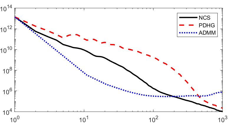
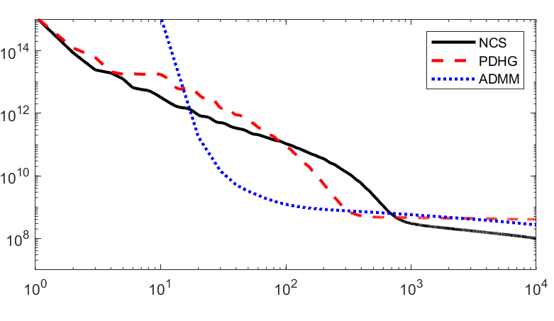
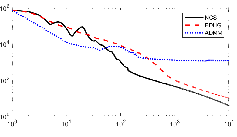
We observe that the matrix-vector multiplication with and dominates the computational cost; the cost of the FFT in NCS and other operations is much smaller in comparison. Consequently, the costs of one iteration of NCS, one iteration of PDHG, and one CG iteration for ADMM are comparable. The convergence plots of Figure 2 show that NCS provides a speedup over PDHG and ADMM. Figure 3 shows reconstructed images. Table 1 shows the speedup of the GPU implementation over the CPU implementation. Time measurements were taken on a system with an Intel Core i7-990X CPU running at 3.47GHz and a Titan Xp GPU.
For parallel beam CT, we use real patient data provided by the Mayo Clinic (referenced in the acknowledgements). For fan beam and cone beam CT, we use the synthetic extended cardiac-torso (XCAT) data [59] and follow the setup of [68]. For PET, we use the data of [41] and follow its setup.
For all experiments, we roughly tuned the parameters of NCS and the other method at a resolution of powers of ; i.e., we tested parameters and for . To get good performance, tuning the parameters well was important, but it was not a very difficult or sensitive process.
Parallel beam CT reconstructs a image with .
The discrete Radon transform computed equiangular projections for a total of measurements.
The matrix-vector multiplication with respect to and were performed with the MATLAB GPU-accelerated radon and iradon functions.
For NCS, we used , , , and .
For PDHG, we used , , and .
For ADMM, we used , , and CG inner iterations per outer loop.
Fan beam CT reconstructs a image with a sinogram of measurements and . The matrix-vector multiplications with respect to and were performed with the MATLAB GPU-accelerated sparse matrices. For NCS, we used , , and . For PDHG, we used , , and . For ADMM, we used , , and CG inner iterations per outer loop.
Cone beam CT reconstructs a 3D image with a sinogram of measurements and . The matrix-vector multiplications with respect to and were performed with Fessler’s MIRT toolbox [24]. For NCS, we used , , and . For PDHG, we used , , and . For ADMM, we used , , and CG inner iterations per outer loop.
PET reconstructs a image with the geometry of equally spaced detectors on the unit circle and . The matrix-vector multiplications with respect to and were performed with MATLAB GPU-accelerated sparse matrices. For NCS, we used , , , and . For PDHG, we used , , and . For ADMM, we used , , and CG inner iterations per outer loop.
For parallel beam CT and PET, where we use circulant approximations based on the analytic formula (13), NCS consistently outperforms PDHG. For fan beam and cone beam CT, where we use circulant approximations based on the more ad hoc formula (15), NCS outperforms PDHG in specific regimes (in early iterations or later iterations). ADMM with CG performs well in early iterations but worse in later iterations.
|
TITAN Xp | Speedup | |||
|---|---|---|---|---|---|
| Par Beam CT ( | x | ||||
| Par Beam CT ( | x | ||||
| Par Beam CT ( | x | ||||
| Par Beam CT ( | x | ||||
| PET | x | ||||
| PET | x | ||||
| PET ( | x |
6 Conclusion
In this paper, we presented NCS, a splitting method that leverages the near-circulant structure present in certain imaging applications. For the problems we consider, ADMM/DRS requires an exact pseudoinverse, which is a significant computational burden. This requirement is relaxed for NCS; we only need to compute the pseudoinverse of an approximate linear system. We theoretically analyzed NCS, and the result informs us of the effect and the advantage of using an approximate pseudoinverse. We presented medical imaging applications that exhibit near-circulant structures, which provide computationally efficient approximate pseudoinverses. We apply NCS to these problems, and, through experiments, empirically validate the theory and demonstrate that the algorithm can effectively utilize the parallel computing capability of a CUDA GPU. The code used for our experiments is available at https://github.com/kose-y/near-circulant-splitting
7 Appendix
In this section, we quickly show how to obtain (ADMM) from ADMM and DRS. The two derivations are, in a sense, equivalent because ADMM and DRS are, in a sense, equivalent methods [26].
7.1 Derivation from ADMM
7.2 Derivation from DRS
Write the dual problem (6) as
Apply DRS to this dual formulation to get
Define with
Then
and
The algorithm depends on only through the product . Therefore, we can write
Acknowledgments
We would like to thank Wotao Yin for his many helpful comments. We gratefully acknowledge the support of NVIDIA Corporation with the donation of the Titan Xp GPU used for this research. We thank Dr. Cynthia McCollough, the Mayo Clinic, the American Association of Physicists in Medicine, and grants EB017095 and EB017185 from the National Institute of Biomedical Imaging and Bioengineering for providing the real patient data used in the experiments.
References
- [1] N. Ahmed, T. Natarajan, and K. R. Rao, Discrete cosine transfom, IEEE Transactions on Computers, C-23 (1974), pp. 90–93.
- [2] M. S. C. Almeida and M. Figueiredo, Deconvolving images with unknown boundaries using the alternating direction method of multipliers, IEEE Transactions on Image Processing, 22 (2013), pp. 3074–3086.
- [3] H. H. Bauschke, R. I. Boţ, W. L. Hare, and W. M. Moursi, Attouch–Théra duality revisited: Paramonotonicity and operator splitting, Journal of Approximation Theory, 164 (2012), pp. 1065–1084.
- [4] H. H. Bauschke and P. L. Combettes, Convex Analysis and Monotone Operator Theory in Hilbert Spaces, Springer New York, 2nd ed., 2017.
- [5] H. H. Bauschke and W. M. Moursi, On the Douglas–Rachford algorithm, Mathematical Programming, 164 (2017), pp. 263–284.
- [6] J. Bian, K. Yang, J. M. Boone, X. Han, E. Y. Sidky, and X. Pan, Investigation of iterative image reconstruction in low-dose breast CT, Physics in Medicine & Biology, 59 (2014), pp. 2659–2685.
- [7] R. I. Boţ, E. R. Csetnek, A. Heinrich, and C. Hendrich, On the convergence rate improvement of a primal-dual splitting algorithm for solving monotone inclusion problems, Mathematical Programming, 150 (2015), pp. 251–279.
- [8] S. Boyd and L. Vandenberghe, Convex Optimization, 2004.
- [9] K. Bredies and H. Sun, Preconditioned Douglas–Rachford algorithms for TV- and TGV-regularized variational imaging problems, Journal of Mathematical Imaging and Vision, 52 (2015), pp. 317–344.
- [10] K. Bredies and H. Sun, Preconditioned Douglas–Rachford splitting methods for convex-concave saddle-point problems, SIAM Journal on Numerical Analysis, 53 (2015), pp. 421–444.
- [11] Y. Cai, M. Donatelli, D. Bianchi, and T.-Z. Huang, Regularization preconditioners for frame-based image deblurring with reduced boundary artifacts, SIAM Journal on Scientific Computing, 38 (2016), pp. B164–B189.
- [12] A. Chambolle, V. Caselles, M. Novaga, D. Cremers, and T. Pock, An introduction to total variation for image analysis, in Theoretical Foundations and Numerical Methods for Sparse Recovery, 2010, pp. 263–340.
- [13] A. Chambolle and T. Pock, A first-order primal-dual algorithm for convex problems with applications to imaging, Journal of Mathematical Imaging and Vision, 40 (2011), pp. 120–145.
- [14] A. Chambolle and T. Pock, On the ergodic convergence rates of a first-order primal-dual algorithm, Mathematical Programming, 159 (2016), pp. 253–287.
- [15] R. H. Chan and M. K. Ng, Conjugate gradient methods for Toeplitz systems, SIAM Review, 38 (1996), pp. 427–482.
- [16] T. F. Chan, An optimal circulant preconditioner for Toeplitz systems, SIAM Journal on Scientific and Statistical Computing, 9 (1988), pp. 766–771.
- [17] K. Choi, J. Wang, L. Zhu, T.-S. Suh, S. Boyd, and L. Xing, Compressed sensing based cone-beam computed tomography reconstruction with a first-order method, Medical Physics, 37 (2010), pp. 5113–5125.
- [18] D. Davis, Convergence rate analysis of primal-dual splitting schemes, SIAM Journal on Optimization, 25 (2015), pp. 1912–1943.
- [19] D. Davis and W. Yin, A three-operator splitting scheme and its optimization applications, Set-Valued and Variational Analysis, 25 (2017), pp. 829–858.
- [20] S. R. Deans, The Radon transform and some of its applications, Wiley Interscience, 1983.
- [21] W. Deng and W. Yin, On the global and linear convergence of the generalized alternating direction method of multipliers, Journal of Scientific Computing, 66 (2016), pp. 889–916.
- [22] J. Douglas and H. H. Rachford, On the numerical solution of heat conduction problems in two and three space variables, Transactions of the American Mathematical Society, 82 (1956), pp. 421–439.
- [23] E. Esser, X. Zhang, and T. F. Chan, A general framework for a class of first order primal-dual algorithms for convex optimization in imaging science, SIAM Journal on Imaging Sciences, 3 (2010), pp. 1015–1046.
- [24] J. A. Fessler, Michigan image reconstruction toolbox. https://web.eecs.umich.edu/~fessler/code/. Accessed: 2019-06-14.
- [25] J. A. Fessler and S. D. Booth, Conjugate-gradient preconditioning methods for shift-variant pet image reconstruction, IEEE Transactions on Image Processing, 8 (1999), pp. 688–699.
- [26] D. Gabay, Applications of the method of multipliers to variational inequalities, in Augmented Lagrangian Methods: Applications to the Numerical Solution of Boundary-Value Problems, M. Fortin and R. Glowinski, eds., 1983.
- [27] D. Gabay and B. Mercier, A dual algorithm for the solution of nonlinear variational problems via finite element approximation, Computers and Mathematics with Applications, 2 (1976), pp. 17–40.
- [28] R. Glowinski and A. Marroco, Sur l’approximation, par éléments finis d’ordre un, et la résolution, par pénalisation-dualité d’une classe de problÚmes de Dirichlet non linéaires, Revue Française d’Automatique, Informatique, Recherche Opérationnelle. Analyse Numérique, 9 (1975), pp. 41–76.
- [29] T. Goldstein and S. Osher, The split Bregman method for l1-regularized problems, SIAM Journal on Imaging Sciences, 2 (2009), pp. 323–343.
- [30] G. H. Golub and C. F. Van Loan, Matrix Computations, 4th ed., 2012.
- [31] M. A. Hasan and C. Negre, Multiway splitting method for Toeplitz matrix vector product, IEEE Transactions on Computers, 62 (2013), pp. 1467–1471.
- [32] R. A. Horn and C. R. Johnson, Matrix Analysis, Cambridge University Press, 2nd ed., 2012.
- [33] J. Huang and T.-Z. Huang, A nonstationary accelerating alternating direction method for frame-based Poissonian image deblurring, Journal of Computational and Applied Mathematics, 352 (2019), pp. 181–193.
- [34] A. K. Jain, Fundamentals of Digital Image Processing, Prentice Hall, 1989.
- [35] A. Katsevich, Theoretically exact filtered backprojection-type inversion algorithm for spiral CT, SIAM Journal on Applied Mathematics, 62 (2002), pp. 2012–2026.
- [36] R. B. Kellogg, A nonlinear alternating direction method, Mathematics of Computation, 23 (1969), pp. 23–27.
- [37] M. A. Krasnosel’skii, Two remarks on the method of successive approximations, Uspekhi Matematicheskikh Nauk, 10 (1955), pp. 123–127.
- [38] K. Lange and R. Carson, EM reconstruction algorithms for emission and transmission tomography, Journal of Computer Assisted Tomography, 8 (1984), pp. 306–16.
- [39] A. J. Laub, Matrix Analysis for Scientists and Engineers, Society for Industrial and Applied Mathematics, 2005.
- [40] T. Lee, J.-H. Won, J. Lim, and S. Yoon, Large-scale structured sparsity via parallel fused lasso on multiple GPUs, Journal of Computational and Graphical Statistics, 26 (2017), pp. 851–864.
- [41] H. Lim, Y. K. Dewaraja, and J. A. Fessler, A PET reconstruction formulation that enforces non-negativity in projection space for bias reduction in Y-90 imaging, Physics in Medicine & Biology, 63 (2018), p. 035042.
- [42] P. L. Lions and B. Mercier, Splitting algorithms for the sum of two nonlinear operators, SIAM Journal on Numerical Analysis, 16 (1979), pp. 964–979.
- [43] W. R. Mann, Mean value methods in iteration, Proceedings of the American Mathematical Society, 4 (1953), pp. 506–510.
- [44] F. Natterer, The Mathematics of Computerized Tomography, Society for Industrial and Applied Mathematics, 2001.
- [45] M. K. Ng, Circulant and skew-circulant splitting methods for Toeplitz systems, Journal of Computational and Applied Mathematics, 159 (2003), pp. 101–108.
- [46] M. K. Ng, R. H. Chan, and W.-C. Tang, A fast algorithm for deblurring models with Neumann boundary conditions, SIAM Journal on Scientific Computing, 21 (1999), pp. 851–866.
- [47] D. O’Connor, Primal-Dual Decomposition by Operator Splitting and Applications to Image Deblurring, PhD thesis, UCLA, 2015.
- [48] D. O’Connor and L. Vandenberghe, Primal-dual decomposition by operator splitting and applications to image deblurring, SIAM Journal on Imaging Sciences, 7 (2014), pp. 1724–1754.
- [49] D. O’Connor and L. Vandenberghe, On the equivalence of the primal-dual hybrid gradient method and Douglas–Rachford splitting, Mathematical Programming, (2018).
- [50] A. V. Oppenheim and R. W. Schafer, Discrete-time signal processing, Prentice Hall, 3rd ed., 2009.
- [51] D. W. Peaceman and H. H. Rachford, The numerical solution of parabolic and elliptic differential equations, Journal of the Society for Industrial and Applied Mathematics, 3 (1955).
- [52] T. Pock and A. Chambolle, Diagonal preconditioning for first order primal-dual algorithms in convex optimization, in Proceedings of the 2011 International Conference on Computer Vision, 2011, pp. 1762–1769.
- [53] T. Pock, D. Cremers, H. Bischof, and A. Chambolle, An algorithm for minimizing the Mumford-Shah functional, IEEE International Conference on Computer Vision, (2009).
- [54] S. Ramani and J. A. Fessler, A splitting-based iterative algorithm for accelerated statistical X-ray CT reconstruction, IEEE Transactions on Medical Imaging, 31 (2012), pp. 677–688.
- [55] R. Rockafellar, Conjugate Duality and Optimization, Society for Industrial and Applied Mathematics, 1974.
- [56] R. T. Rockafellar, Convex Analysis, 1970.
- [57] L. I. Rudin, S. Osher, and E. Fatemi, Nonlinear total variation based noise removal algorithms, Physica D: Nonlinear Phenomena, 60 (1992), pp. 259–268.
- [58] E. K. Ryu and S. Boyd, Primer on monotone operator methods, Applied and Computational Mathematics, 15 (2016), pp. 3–43.
- [59] W. P. Segarsa, M. Mahesh, T. J. Beck, E. C. Frey, and B. M. W. Tsui, Realistic CT simulation using the 4D XCAT phantom, Medical Physics, 35 (2008), pp. 3800–3808.
- [60] L. A. Shepp and Y. Vardi, Maximum likelihood reconstruction for emission tomography, IEEE Transactions on Medical Imaging, 1 (1982), pp. 113–122.
- [61] E. Y. Sidky, J. H. Jørgensen, and X. Pan, Convex optimization problem prototyping for image reconstruction in computed tomography with the Chambolle–Pock algorithm, Physics in Medicine & Biology, 57 (2012), pp. 3065–3091.
- [62] G. Strang, A proposal for Toeplitz matrix calculations, Studies in Applied Mathematics, 74 (1986), pp. 171–176.
- [63] G. Strang, The discrete cosine transform, SIAM Review, 41 (1999), pp. 135–147.
- [64] P. Toft, The Radon Transform: Theory and Implementation, PhD thesis, Technical University of Denmark, 1996.
- [65] Y. Vardi, L. Shepp, and L. Kaufman, A statistical model for positron emission tomography, Journal of the American Statistical Association, 80 (1985), pp. 8–20.
- [66] Z.-J. Xie, X.-Q. Jin, and Y.-M. Wei, A fast algorithm for solving circulant tensor systems, Linear and Multilinear Algebra, 65 (2017), pp. 1894–1904.
- [67] X.-L. Zhao, F. Wang, T.-Z. Huang, M. K. Ng, and R. J. Plemmons, Deblurring and sparse unmixing for hyperspectral images, IEEE Transactions on Geoscience and Remote Sensing, 51 (2013), pp. 4045–4058.
- [68] X. Zheng, S. Ravishankar, Y. Long, and J. A. Fessler, PWLS-ULTRA: An efficient clustering and learning-based approach for low-dose 3D CT image reconstruction, IEEE Transactions on Medical Imaging, 37 (2018), pp. 1498–1510.
- [69] M. Zhu and T. Chan, An efficient primal-dual hybrid gradient algorithm for total variation image restoration, UCLA CAM Report 08-34, (2008).