跳到论文正文
W Papers独立论文阅读器 arXiv:1810.11904 论文正文 计算阅读时间 · 0%
引用这篇论文根据当前论文元数据生成,正式投稿前建议核对。


License: arXiv.org perpetual non-exclusive license
arXiv:1810.11904v1 [math.PR] 28 Oct 2018

Eigenvalue Fluctuations of Symmetric Group Permutation Representations on k-tuples and k-subsets

Benjamin Tsou Address: Department of Mathematics, University of California, Berkeley, CA 94720-3840 Email address: benjamintsou@gmail.com
Abstract.

Let the term kk-representation refer to the permutation representations of the symmetric group 𝔖n\mathfrak{S}_{n} on kk-tuples and kk-subsets as well as the S(n−k,1k)S^{(n-k,1^{k})} irreducible representation of 𝔖n\mathfrak{S}_{n}. Endow 𝔖n\mathfrak{S}_{n} with the Ewens distribution and let α\alpha and β\beta be linearly independent irrational numbers over ℚ\mathbb{Q}. Then for fixed k>1k>1 we show that as n→∞n\to\infty, the normalized count of the number of eigenangles in a fixed interval (α,β)(\alpha,\beta) of a kk-representation evaluated at a random element σ∈𝔖n\sigma\in\mathfrak{S}_{n} converges weakly to a compactly supported distribution. In particular, we compute the limiting moments and moreover provide an explicit formula for the limiting density when k=2k=2 and the Ewens parameter θ=1\theta=1 (uniform probability measure). This is in contrast to the k=1k=1 case where it has been shown previously that the distribution is asymptotically Gaussian.

1. Introduction

The group of permutation matrices can be viewed as the simplest (nontrivial) permutation representation of the symmetric group 𝔖n\mathfrak{S}_{n}. Wieand [30] showed that under a uniform probability measure, the normalized limiting distribution of the number of eigenvalues of a random permutation matrix in some fixed arc of the unit circle follows a standard normal distribution. Recently, Ben Arous and Dang [5] have extended Wieand’s work in [30] to general functions other than the indicator function on an interval. In particular, they show that the fluctuations of sufficiently smooth linear statistics of permutation matrices drawn from the Ewens distribution are asymptotically non-Gaussian but infinitely divisible. They mention that this result is quite unusual since most prior work show asymptotic Gaussianity of eigenvalue fluctuation statistics.

In this paper, we extend Wieand’s results in a different direction by studying higher dimensional representations of the symmetric group. In particular, we will consider the permutation representations on ordered kk-tuples and unordered subsets of size kk as well as the irreducible representation S(n−k,1k)S^{(n-k,1^{k})} for k≥2k\geq 2. We show that for these three types of representations (denoted ρn,ktuple\rho_{n,k}^{\textrm{tuple}}, ρn,kset\rho_{n,k}^{\textrm{set}}, and ρ(n−k,1k)\rho^{(n-k,1^{k})}), for σ∈𝔖n\sigma\in\mathfrak{S}_{n} drawn from the Ewens distribution, the normalized count of eigenvalues in some fixed arc of the unit circle converges to a class of compactly supported limiting distributions.

Let us now quickly review how permutation representations of kk-tuples and kk-subsets are defined. Section 4 will give a short overview of irreducible representations of symmetric groups.

First, consider the set Qn,ktupleQ_{n,k}^{\textrm{tuple}} of ordered kk-tuples (t1,…,tk)(t_{1},...,t_{k}) of distinct integers chosen from the set [n]:={1,…,n}[n]\mathrel{\mathop{\mathchar 58\relax}}=\{1,...,n\}. The symmetric group 𝔖n\mathfrak{S}_{n} acts naturally on this set by σ⁡(t1,…,tk)=(σ⁡(t1),…,σ⁡(tk))\sigma(t_{1},...,t_{k})=(\sigma(t_{1}),...,\sigma(t_{k})). We can form the n!(n−k)!\displaystyle{\frac{n!}{(n-k)!}}-dimensional vector space Vn,ktupleV_{n,k}^{\textrm{tuple}} with basis elements e(t1,…,tk)e_{(t_{1},...,t_{k})}. Then the action of 𝔖n\mathfrak{S}_{n} on Qn,ktupleQ_{n,k}^{\textrm{tuple}} induces the permutation representation ρn,ktuple:𝔖n→O⁡(Vn,ktuple)\rho_{n,k}^{\textrm{tuple}}\mathrel{\mathop{\mathchar 58\relax}}\mathfrak{S}_{n}\rightarrow O(V_{n,k}^{\textrm{tuple}}) where O⁡(Vn,ktuple)O(V_{n,k}^{\textrm{tuple}}) is the orthogonal group on Vn,ktupleV_{n,k}^{\textrm{tuple}}.

Similarly, consider the set Qn,ksetQ_{n,k}^{\textrm{set}} of kk-subsets {t1,…,tk}\{t_{1},...,t_{k}\} of distinct integers chosen from [n][n]. As for the set of ordered tuples, the symmetric group 𝔖n\mathfrak{S}_{n} acts naturally on Qn,ksetQ_{n,k}^{\textrm{set}} by σ⁡({t1,…,tk})={σ⁡(t1),…,σ⁡(tk)}\sigma(\{t_{1},...,t_{k}\})=\{\sigma(t_{1}),...,\sigma(t_{k})\}. We can form the (nk)\displaystyle{\binom{n}{k}}-dimensional vector space Vn,ksetV_{n,k}^{\textrm{set}} with basis elements e{t1,…,tk}e_{\{t_{1},...,t_{k}\}}. Then the action of 𝔖n\mathfrak{S}_{n} on Qn,ksetQ_{n,k}^{\textrm{set}} gives the permutation representation ρn,kset:𝔖n→O⁡(Vn,kset)\rho_{n,k}^{\textrm{set}}\mathrel{\mathop{\mathchar 58\relax}}\mathfrak{S}_{n}\to O(V_{n,k}^{\textrm{set}}).

To state the main results, let us introduce the relevant random variables describing the eigenvalue statistics of these symmetric group representations. Finite group representations are all unitarisable, and therefore all the eigenvalues are of the form e2​π​i​ϕe^{2\pi i\phi} on the unit circle. It will be convenient to refer to each eigenvalue e2​π​i​ϕe^{2\pi i\phi} by its eigenangle ϕ∈[0,1)\phi\in[0,1). Let I=(α,β)I=(\alpha,\beta) be an interval where α\alpha and β\beta are irrational and linearly independent over ℚ\mathbb{Q}. For σ∈𝔖n\sigma\in\mathfrak{S}_{n}, let Xn,ktuple​(σ)X_{n,k}^{\textrm{tuple}}(\sigma), Xn,kset​(σ)X_{n,k}^{\textrm{set}}(\sigma), and Xn,kirrep​(σ)X_{n,k}^{\textrm{irrep}}(\sigma) denote the number of eigenangles (counted with multiplicity) of ρn,ktuple​(σ)\rho_{n,k}^{\textrm{tuple}}(\sigma), ρn,kset​(σ)\rho_{n,k}^{\textrm{set}}(\sigma), and ρ(n−k,1k)​(σ)\rho^{(n-k,1^{k})}(\sigma) respectively in the arc II.

Recall (see e.g. [15]) that the Ewens distribution with parameter θ>0\theta>0 defined on 𝔖n\mathfrak{S}_{n} is given by

(1.1) ℙ⁡(σ)=θK⁡(σ)θ(θ+1)⋯(θ+n−1)\mathbb{P}(\sigma)=\frac{\theta^{K(\sigma)}}{\theta(\theta+1)\cdot\cdot\cdot(\theta+n-1)}

where K⁡(σ)K(\sigma) is the total number of cycles of the permutation σ\sigma. By equipping 𝔖n\mathfrak{S}_{n} with the Ewens measure, we can think of Xn,ktupleX_{n,k}^{\textrm{tuple}}, Xn,ksetX_{n,k}^{\textrm{set}}, and Xn,kirrepX_{n,k}^{\textrm{irrep}} as random variables.

For k>1k>1, define the centered and scaled versions

(1.2) Yn,ktuple:=Xn,ktuple−𝔼⁡[Xn,ktuple]nk−1Y_{n,k}^{\textrm{tuple}}\mathrel{\mathop{\mathchar 58\relax}}=\frac{X_{n,k}^{\textrm{tuple}}-\mathbb{E}[X_{n,k}^{\textrm{tuple}}]}{n^{k-1}}
(1.3) Yn,kset:=k!​Xn,kset−𝔼⁡[Xn,kset]nk−1Y_{n,k}^{\textrm{set}}\mathrel{\mathop{\mathchar 58\relax}}=k!\frac{X_{n,k}^{\textrm{set}}-\mathbb{E}[X_{n,k}^{\textrm{set}}]}{n^{k-1}}
(1.4) Yn,kirrep:=k!​Xn,kirrep−𝔼⁡[Xn,kirrep]nk−1Y_{n,k}^{\textrm{irrep}}\mathrel{\mathop{\mathchar 58\relax}}=k!\frac{X_{n,k}^{\textrm{irrep}}-\mathbb{E}[X_{n,k}^{\textrm{irrep}}]}{n^{k-1}}

Our first result is to show that to compute the limiting distribution of these normalized eigenangle counts, it suffices to consider the simpler random variables Yn,kY_{n,k} defined below. For each σ∈𝔖n\sigma\in\mathfrak{S}_{n}, let Cj(n)​(σ)C_{j}^{(n)}(\sigma) denote the number of cycles of σ\sigma of length jj. Let ℒ⁡(X)\mathcal{L}(X) denote the law of a random variable XX.

Theorem 1.1.

Let

(1.5) Yn,k=∑j=1njk−1​Cj(n)​({j​α}−{j​β})nk−1Y_{n,k}=\sum_{j=1}^{n}\frac{j^{k-1}C_{j}^{(n)}(\{j\alpha\}-\{j\beta\})}{n^{k-1}}

Under the Ewens distribution with parameter θ>0\theta>0, as n→∞n\to\infty for fixed k>1k>1, each of the random variables Yn,ktupleY_{n,k}^{\textrm{tuple}}, Yn,ksetY_{n,k}^{\textrm{set}}, and Yn,kirrepY_{n,k}^{\textrm{irrep}} converges in law to the same limiting distribution limn→∞ℒ⁡(Yn,k)\displaystyle{\lim_{n\to\infty}\mathcal{L}(Y_{n,k})} (assuming it exists).

Remark 1.1.

In fact, the proof of Theorem 1.1 readily shows that a similar result stated in Theorem 9.3 holds for more general linear eigenvalue statistics than the indicator of an interval.

Since ∑j=1nj​Cj(n)=n\displaystyle{\sum_{j=1}^{n}jC_{j}^{(n)}=n}, it is easy to see that ∑j=1njk−1​Cj(n)≤nk−1\displaystyle{\sum_{j=1}^{n}j^{k-1}C_{j}^{(n)}\leq n^{k-1}}. Thus, the distribution of Yn,kY_{n,k} is supported on the finite interval [−1,1][-1,1] for all nn. Hence by the method of moments, the sequence converges in distribution as long as the moments converge. The following theorem gives the limiting moments implicitly in terms of the exponential of a formal power series.

Theorem 1.2.

Under the Ewens distribution with parameter θ>0\theta>0, for k>1k>1, Yn,kY_{n,k} converges weakly as n→∞n\to\infty to some compactly supported limiting distribution Y∞,kY_{\infty,k}. The moments of Y∞,kY_{\infty,k} are given implicitly by the following equation in formal power series:

(1.6) ∑m=0∞𝔼⁡[(Y∞,k)m]​Γ⁡(m⁡(k−1)+θ)Γ⁡(θ)​m!​zm=exp⁡(K⁡(z))\sum_{m=0}^{\infty}\mathbb{E}[(Y_{\infty,k})^{m}]\frac{\Gamma(m(k-1)+\theta)}{\Gamma(\theta)m!}z^{m}=\exp(K(z))

where K⁡(z)=∑m=1∞κ2​m​z2​m\displaystyle{K(z)=\sum_{m=1}^{\infty}\kappa_{2m}z^{2m}} and κ2​m=2​θ​(2​m​(k−1)−1)!(2​m+2)!\displaystyle{\kappa_{2m}=\frac{2\theta(2m(k-1)-1)!}{(2m+2)!}}.

Remarkably, when k=2k=2 and θ=1\theta=1, an explicit formula for the density of Y∞,2Y_{\infty,2} can be obtained.

Corollary 1.1.

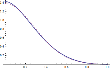
For θ=1\theta=1 (i.e. the uniform measure on 𝔖n\mathfrak{S}_{n}), the random variable Y∞,2Y_{\infty,2} is supported on the interval [−1,1][-1,1] and has probability density given by the formula:

(1.7) pY∞,2​(t)=e3/2π​|t|​(1|t|−1)−12​(1−|t|)2​(1|t|+1)−12​(1+|t|)2​sin⁡((1−|t|)22​π)p_{Y_{\infty,2}}(t)=\frac{e^{3/2}}{\pi|t|}\left(\frac{1}{|t|}-1\right)^{-\frac{1}{2}(1-|t|)^{2}}\left(\frac{1}{|t|}+1\right)^{-\frac{1}{2}(1+|t|)^{2}}\sin\bigg(\frac{(1-|t|)^{2}}{2}\pi\bigg)

for −1≤t≤1-1\leq t\leq 1 (and by continuity, 𝑂𝑃𝐸𝑁pY∞,2​(0)=e3/2π)\displaystyle{p_{Y_{\infty,2}}(0)=\frac{e^{3/2}}{\pi}}\bigg).

The rest of the paper is organized as follows. In sections 2, 3, and 4, we prove Theorem 1.1 in turn for Yn,ktupleY_{n,k}^{\textrm{tuple}}, Yn,ksetY_{n,k}^{\textrm{set}}, and Yn,kirrepY_{n,k}^{\textrm{irrep}}. In section 5, we review some basic theory of equidistributed sequences that will be useful for the moment method. In section 6, we use the method of moments to rederive the asymptotic gaussianity of the normalized eigenangle count in the k=1k=1 case of permutation matrices. Then we move on to the k>1k>1 case and prove Theorem 1.2 in Section 7. Section 8 proves the density formula for k=2k=2 in Corollary 1.1. Finally in Section 9, we discuss the extension of Theorem 1.1 to more general linear eigenvalue statistics and connect our results to those in [5].

We end this introduction with a few bibliographic comments regarding the increasing activity in the study of eigenvalues of random permutation matrices over the last two decades. Wieand extended her Gaussianity results in [30] to wreath products in [31]. Works by Diaconis and Shahshahani [11] and Evans [13] show that the spectrum of permutation matrices and various wreath products under a uniform probability measure converges weakly to the uniform distribution on the circle. Characteristic polynomials associated to a random permutation matrix were studied in several works, including [8], [3], [17], [32], and [9]. Najnudel and Nikeghbali [21] and more recently Bahier ([4], [2]) extend the work of Diaconis, Evans, and Wieand by studying “randomized” permutation matrices where each matrix entry equal to 1 is replaced by i.i.d. variables taking values in ℂ∗\mathbb{C}^{*}. The authors in [18] study a more general Ewens measure than the one considered by Ben Arous and Dang [5] and in this paper, also obtaining eigenvalue statistics fluctuation results. Evans [14] considers spectra of random matrices involving more general representations of the symmetric group 𝔖n\mathfrak{S}_{n}, but the situation is quite different from ours in that the randomness is not taken over 𝔖n\mathfrak{S}_{n}.

2. The kk-tuple representations

In this section, we give a proof of Theorem 1.1 for Yn,ktupleY_{n,k}^{\textrm{tuple}}. First, we give a simple characterization of the spectrum of ρn,ktuple​(σ)\rho_{n,k}^{\textrm{tuple}}(\sigma) for σ∈𝔖n\sigma\in\mathfrak{S}_{n}. Note that the eigenvalues only depend on the cycle structure of σ\sigma since conjugacy classes in 𝔖n\mathfrak{S}_{n} are determined by the cycle structure.

When k=1k=1 (the defining representation of 𝔖n\mathfrak{S}_{n}), ρn,1tuple​(σ)=M\rho_{n,1}^{\textrm{tuple}}(\sigma)=M where MM is the permutation matrix corresponding to σ\sigma, i.e. Mi​j=1M_{ij}=1 if j=σ⁡(i)j=\sigma(i) and 0 otherwise. It is easy to see that each jj-cycle in σ\sigma corresponds to the set of jj eigenangles {0,1j,…,j−1j}\displaystyle{\left\{0,\frac{1}{j},...,\frac{j-1}{j}\right\}}. For each jj, we have Cj(n)​(σ)C_{j}^{(n)}(\sigma) copies of these eigenangles.

Then

(2.1) Xn,1tuple​(σ)=n⁡(β−α)+∑j=1nCj(n)​(σ)​({j​α}−{j​β})X_{n,1}^{\textrm{tuple}}(\sigma)=n(\beta-\alpha)+\sum_{j=1}^{n}C_{j}^{(n)}(\sigma)(\{j\alpha\}-\{j\beta\})

where {x}\{x\} denotes the fractional part of xx.

More generally, ρn,ktuple​(σ)\rho_{n,k}^{\textrm{tuple}}(\sigma) is the n!(n−k)!×n!(n−k)!\displaystyle{\frac{n!}{(n-k)!}\times\frac{n!}{(n-k)!}} permutation matrix MM corresponding to the action of σ\sigma on Vn,ktupleV_{n,k}^{\textrm{tuple}}. Here, M(t1,…,tk),(u1,…,uk)=1M_{(t_{1},...,t_{k}),(u_{1},...,u_{k})}=1 if (u1,…,uk)=σ⁡(t1,…,tk)(u_{1},...,u_{k})=\sigma(t_{1},...,t_{k}) and 0 otherwise. Let σktuple\sigma_{k}^{\textrm{tuple}} be the permutation of size n!(n−k)!\displaystyle{\frac{n!}{(n-k)!}} corresponding to MM. Then looking at the cycle structure, we have

(2.2) Xn,ktuple​(σ)=n!(n−k)!​(β−α)+∑jCj,k(n),tuple​(σ)​({j​α}−{j​β})X_{n,k}^{\textrm{tuple}}(\sigma)=\frac{n!}{(n-k)!}(\beta-\alpha)+\sum_{j}C_{j,k}^{(n),\textrm{tuple}}(\sigma)(\{j\alpha\}-\{j\beta\})

where Cj,k(n),tuple​(σ)C_{j,k}^{(n),\textrm{tuple}}(\sigma) is the number of cycles in σktuple\sigma_{k}^{\textrm{tuple}} of length jj.

We will say that an integer ii lies in cycle CC of the permutation σ\sigma if CC contains ii in the cycle decomposition of σ\sigma. It will turn out that almost all the contribution to the sum in Yn,ktupleY_{n,k}^{\textrm{tuple}} comes from the tuples (OPENt1,…,tk)t_{1},...,t_{k}) such that t1,…,tkt_{1},...,t_{k} all lie in the same cycle of σ\sigma.

Remark 2.1.

To reduce confusion, we will sometimes use the terms σ\sigma-cycle and σktuple\sigma_{k}^{\textrm{tuple}}-cycle to distinguish between cycles of σ\sigma and σktuple\sigma_{k}^{\textrm{tuple}} respectively.

Remark 2.2.

To reduce clutter, we will often leave the index off set and sequence notations. For example, if the index nn is understood to run over the range 1≤n≤N1\leq n\leq N, then the notation (an)(a_{n}) should be read as the sequence (a1,…,aN)(a_{1},...,a_{N}). Similarly, if the index ii is understood to run over the range 1≤i≤m1\leq i\leq m, then {Ai}\{A_{i}\} should be read as the set {A1,…,Am}\{A_{1},...,A_{m}\}.

In order to analyze the sum in Yn,ktupleY_{n,k}^{\textrm{tuple}}, it will help to obtain a partition of the set of kk-tuples (t1,…,tk)(t_{1},...,t_{k}) defined by the orbits of the action of σ∈𝔖n\sigma\in\mathfrak{S}_{n}. First, we make the following:

Definition 2.1.

Let [k]=∪i=1mAi\displaystyle{[k]=\mathop{\cup}_{i=1}^{m}A_{i}} be a partition of [k][k] into disjoint, nonempty subsets. Order the sets AiA_{i} such that |A1|≥…≥|Am|>0|A_{1}|\geq...\geq|A_{m}|>0. Setting ki=|Ai|k_{i}=|A_{i}|, this determines an integer partition k=k1+…+kmk=k_{1}+...+k_{m}. Further partition each subset ArA_{r} into p⁡(r)p(r) disjoint, nonempty subsets Ar​sA_{rs} such that |Ar​1|≥…≥|Ar,p⁡(r)|>0|A_{r1}|\geq...\geq|A_{r,p(r)}|>0. This determines an integer partition kr=∑s=1p⁡(r)kr​s\displaystyle{k_{r}=\sum_{s=1}^{p(r)}k_{rs}}. The pair ({Ai},{Ar​s})(\{A_{i}\},\{A_{rs}\}) will be called a double partition of [k][k].

We can now define the following subsets of Qn,ktupleQ_{n,k}^{\textrm{tuple}}:

Definition 2.2.

Let ({Ai},{Ar​s})(\{A_{i}\},\{A_{rs}\}) be a double partition of [k][k] such that |{Ai}|=m|\{A_{i}\}|=m. Choose a sequence (i1,…,im)(i_{1},...,i_{m}) of distinct integers from [n][n]. Then let T{Ai},{Ar​s}σ,(ij)T_{\{A_{i}\},\{A_{rs}\}}^{\sigma,(i_{j})} denote the set of kk-tuples (t1,…,tk)(t_{1},...,t_{k}) of distinct integers such that the integers tjt_{j} where j∈Arj\in A_{r} are all in σ\sigma-cycles of length iri_{r} and moreover, integers tat_{a} and tbt_{b} are in the same σ\sigma-cycle of length iri_{r} iff aa and bb are in the same subset Ar​sA_{rs} of ArA_{r}. Taking the union over σ\sigma-cycle lengths, we also define

(2.3) T{Ai},{Ar​s}σ=⋃i1≠…≠imT{Ai},{Ar​s}σ,(ij)T_{\{A_{i}\},\{A_{rs}\}}^{\sigma}=\bigcup_{i_{1}\neq...\neq i_{m}}T_{\{A_{i}\},\{A_{rs}\}}^{\sigma,(i_{j})}

where i1≠…≠imi_{1}\neq...\neq i_{m} is shorthand for i1,…,imi_{1},...,i_{m} all distinct.

For each σ∈𝔖n\sigma\in\mathfrak{S}_{n}, the set {T{Ai},{Ar​s}σ:({Ai},{Ar​s}) a double partition of [k]}\Big\{T_{\{A_{i}\},\{A_{rs}\}}^{\sigma}\mathrel{\mathop{\mathchar 58\relax}}(\{A_{i}\},\{A_{rs}\})\text{ a double partition of }[k]\Big\} forms a partition of Qn,ktupleQ_{n,k}^{\textrm{tuple}}. Note that the number of parts in this partition is only a function of kk and does not grow with nn. Thus, we can consider separately the limiting contribution of each part T{Ai},{Ar​s}σT_{\{A_{i}\},\{A_{rs}\}}^{\sigma} to the spectrum of ρn,ktuple​(σ)\rho_{n,k}^{\textrm{tuple}}(\sigma).

It is clear that σktuple\sigma_{k}^{\textrm{tuple}} acts on T{Ai},{Ar​s}σ,(ij)T_{\{A_{i}\},\{A_{rs}\}}^{\sigma,(i_{j})} and that each tuple (t1,…,tk)∈T{Ai},{Ar​s}σ,(ij)(t_{1},...,t_{k})\in T_{\{A_{i}\},\{A_{rs}\}}^{\sigma,(i_{j})} lies in a σktuple\sigma_{k}^{\textrm{tuple}}-cycle of length [i1,…,im][i_{1},...,i_{m}]. (Here, [i1,…,im][i_{1},...,i_{m}] denotes the least common multiple of integers i1,…,imi_{1},...,i_{m}). Thus, for each choice of double partition ({Ai},{Ar​s})(\{A_{i}\},\{A_{rs}\}) and each sequence of σ\sigma-cycle lengths (i1,…,im)(i_{1},...,i_{m}), the elements of T{Ai},{Ar​s}σ,(ij)T_{\{A_{i}\},\{A_{rs}\}}^{\sigma,(i_{j})} form

(2.4) 1[i1,…,im]​∏r=1m(Cir(n)​(σ))p⁡(r)¯​∏s=1p⁡(r)irkr​s¯\frac{1}{[i_{1},...,i_{m}]}\prod_{r=1}^{m}\big(C_{i_{r}}^{(n)}(\sigma)\big)^{\underline{p(r)}}\prod_{s=1}^{p(r)}i_{r}^{\underline{k_{rs}}}

σktuple\sigma_{k}^{\textrm{tuple}}-cycles of size [i1,…,im][i_{1},...,i_{m}] where the polynomial xn¯:=x⁡(x−1)​…​(x−n+1)x^{\underline{n}}\mathrel{\mathop{\mathchar 58\relax}}=x(x-1)...(x-n+1) (often called the nnth falling factorial).

The following lemma shows that the only non-negligible contribution to Yn,ktupleY_{n,k}^{\textrm{tuple}} in the limit n→∞n\to\infty comes from the σktuple\sigma_{k}^{\textrm{tuple}}-cycles containing tuples (t1,…,tk)(t_{1},...,t_{k}) such that t1,…,tkt_{1},...,t_{k} are all in the same σ\sigma-cycle.

Lemma 2.1.

Let ({Ai},{Ar​s})(\{A_{i}\},\{A_{rs}\}) be a double partition of [k][k]. If ∑r=1mp⁡(r)>1\displaystyle{\sum_{r=1}^{m}p(r)>1}, then

(2.5) limn→∞1nk−1​𝔼​[∑i1≠…≠im1[i1,…,im]​∏r=1m(Cir(n))p⁡(r)¯​∏s=1p⁡(r)irkr​s¯]=0\lim_{n\to\infty}\frac{1}{n^{k-1}}\mathbb{E}\bigg[\sum_{i_{1}\neq...\neq i_{m}}\frac{1}{[i_{1},...,i_{m}]}\prod_{r=1}^{m}\big(C_{i_{r}}^{(n)}\big)^{\underline{p(r)}}\prod_{s=1}^{p(r)}i_{r}^{\underline{k_{rs}}}\bigg]=0
Proof.

First, we compute the expectation 𝔼⁡[∏r=1m(Cir(n))p⁡(r)¯]\displaystyle{\mathbb{E}\bigg[\prod_{r=1}^{m}\big(C_{i_{r}}^{(n)}\big)^{\underline{p(r)}}\bigg]}, often referred to as a factorial moment.

The following moment formula was established by Watterson [29] (see e.g. [1, (5.6)]): Let W1,…,WnW_{1},...,W_{n} be independent Poisson random variables with 𝔼⁡[Wi]=θ/i\mathbb{E}[W_{i}]=\theta/i and b1,…,bnb_{1},...,b_{n} be non-negative integers and set l=b1+2​b2+…+n​bnl=b_{1}+2b_{2}+...+nb_{n}. Then

(2.6) 𝔼⁡[∏j=1n(Cj(n))bj¯]=𝟙​(l≤n)​𝔼​[∏j=1nWjbj¯]​∏i=0l−1n−iθ+n−i−1\mathbb{E}\bigg[\prod_{j=1}^{n}(C_{j}^{(n)})^{\underline{b_{j}}}\bigg]=\mathds{1}(l\leq n)\mathbb{E}\bigg[\prod_{j=1}^{n}W_{j}^{\underline{b_{j}}}\bigg]\prod_{i=0}^{l-1}\frac{n-i}{\theta+n-i-1}

Also, recall that if XX follows a Poisson distribution with parameter λ\lambda, the factorial moments are given by 𝔼⁡[Xn¯]=λn\mathbb{E}[X^{\underline{n}}]=\lambda^{n}.

Using these results, we can now compute the expectation in the lemma. Note that

∏i=0l−1n−iθ+n−i−1≤nn−l+θ\prod_{i=0}^{l-1}\frac{n-i}{\theta+n-i-1}\leq\frac{n}{n-l+\theta}

Then summing over all sequences (i1,…,im)(i_{1},...,i_{m}) of distinct integers in [n][n], we get (assuming ∑r=1mp⁡(r)>1\displaystyle{\sum_{r=1}^{m}p(r)>1})

𝔼⁡[∑i1≠…≠im1[i1,…,im]​∏r=1m(Cir(n))p⁡(r)¯​∏s=1p⁡(r)irkr​s¯]\displaystyle\mathbb{E}\bigg[\sum_{i_{1}\neq...\neq i_{m}}\frac{1}{[i_{1},...,i_{m}]}\prod_{r=1}^{m}\big(C_{i_{r}}^{(n)}\big)^{\underline{p(r)}}\prod_{s=1}^{p(r)}i_{r}^{\underline{k_{rs}}}\bigg]
≤\displaystyle\leq ∑i1≠…≠im1[i1,…,im]​nn−∑ir​p​(r)+θ​∏r=1m(θir)p⁡(r)​∏s=1p⁡(r)irkr​s\displaystyle\sum_{i_{1}\neq...\neq i_{m}}\frac{1}{[i_{1},...,i_{m}]}\frac{n}{n-\sum i_{r}p(r)+\theta}\prod_{r=1}^{m}\left(\frac{\theta}{i_{r}}\right)^{p(r)}\prod_{s=1}^{p(r)}i_{r}^{k_{rs}}
(2.7) ≤\displaystyle\leq A⁡(θ)​∑i1≠…≠im∑ir​p​(r)<n1[i1,…,im]​nn−∑ir​p​(r)​∏r=1mirkr−p⁡(r)\displaystyle A(\theta)\sum_{\begin{subarray}{c}i_{1}\neq...\neq i_{m}\\ \sum i_{r}p(r)<n\end{subarray}}\frac{1}{[i_{1},...,i_{m}]}\frac{n}{n-\sum i_{r}p(r)}\prod_{r=1}^{m}i_{r}^{k_{r}-p(r)}

for some constant A⁡(θ)A(\theta).

If m=1m=1, splitting the sum according to whether n−i1​p​(1)>nn-i_{1}p(1)>\sqrt{n} or n−∑i1​p​(1)≤nn-\sum i_{1}p(1)\leq\sqrt{n} shows that (2.7) is clearly of order O⁡(nk−3/2)O(n^{k-3/2}) and the lemma follows. If m>1m>1, we have (using the notation (i,j):=gcd⁡(i,j)(i,j)\mathrel{\mathop{\mathchar 58\relax}}=\gcd(i,j) )

∑i1≠…≠im∑ir​p​(r)<n1[i1,…,im]​nn−∑ir​p​(r)​∏r=1mirkr−p⁡(r)\displaystyle\sum_{\begin{subarray}{c}i_{1}\neq...\neq i_{m}\\ \sum i_{r}p(r)<n\end{subarray}}\frac{1}{[i_{1},...,i_{m}]}\frac{n}{n-\sum i_{r}p(r)}\prod_{r=1}^{m}i_{r}^{k_{r}-p(r)}
≤\displaystyle\leq ∑i1≠…≠im∑ir​p​(r)<n1[i1,i2]​nn−∑ir​p​(r)​∏r=1mirkr−p⁡(r)\displaystyle\sum_{\begin{subarray}{c}i_{1}\neq...\neq i_{m}\\ \sum i_{r}p(r)<n\end{subarray}}\frac{1}{[i_{1},i_{2}]}\frac{n}{n-\sum i_{r}p(r)}\prod_{r=1}^{m}i_{r}^{k_{r}-p(r)}
<\displaystyle< nk−k1−k2+1/2​∑i≠jik1−1​jk2−1[i,j]\displaystyle\;n^{k-k_{1}-k_{2}+1/2}\sum_{i\neq j}\frac{i^{k_{1}-1}j^{k_{2}-1}}{[i,j]}
=\displaystyle=  2​nk−k1−k2+1/2​∑1≤i<j≤nik1−2​jk2−2​(i,j)\displaystyle\;2n^{k-k_{1}-k_{2}+1/2}\sum_{1\leq i<j\leq n}i^{k_{1}-2}j^{k_{2}-2}(i,j)
=\displaystyle=  2​nk−k1−k2+1/2​∑1≤i<j≤n(i,j)=1∑d≤nj(d​i)k1−2​(d​j)k2−2​d\displaystyle\;2n^{k-k_{1}-k_{2}+1/2}\sum_{\begin{subarray}{c}1\leq i<j\leq n\\ (i,j)=1\end{subarray}}\sum_{d\leq\frac{n}{j}}(di)^{k_{1}-2}(dj)^{k_{2}-2}d
<\displaystyle<  2​nk−k1−k2+1/2​∑1≤i<j≤n∑d≤njdk1+k2−3​ik1−2​jk2−2\displaystyle\;2n^{k-k_{1}-k_{2}+1/2}\sum_{1\leq i<j\leq n}\sum_{d\leq\frac{n}{j}}d^{k_{1}+k_{2}-3}i^{k_{1}-2}j^{k_{2}-2}
<\displaystyle<  2​nk−k1−k2+1/2​∑i=1n∑j=in(nj)k1+k2−2​ik1−2​jk2−2\displaystyle\;2n^{k-k_{1}-k_{2}+1/2}\sum_{i=1}^{n}\sum_{j=i}^{n}\left(\frac{n}{j}\right)^{k_{1}+k_{2}-2}i^{k_{1}-2}j^{k_{2}-2}
<\displaystyle<  2​nk−3/2​∑i=1n∑j=inik1−2jk1\displaystyle\;2n^{k-3/2}\sum_{i=1}^{n}\sum_{j=i}^{n}\frac{i^{k_{1}-2}}{j^{k_{1}}}

Here, the second step is derived by splitting the sum according to whether n−∑ir​p​(r)>nn-\sum i_{r}p(r)>\sqrt{n} or n−∑ir​p​(r)≤nn-\sum i_{r}p(r)\leq\sqrt{n}. The desired result then follows from the fact that

∑i=1n∑j=inik1−2jk1=O⁡(log2⁡n)\sum_{i=1}^{n}\sum_{j=i}^{n}\frac{i^{k_{1}-2}}{j^{k_{1}}}=O(\log^{2}n)

∎

Lemma 2.1 shows that the only cycles of σktuple\sigma_{k}^{\textrm{tuple}} that contribute to Yn,ktupleY_{n,k}^{\textrm{tuple}} in the limit n→∞n\to\infty are those formed from tuples in the set T{Ai},{Ar​s}σT_{\{A_{i}\},\{A_{rs}\}}^{\sigma} such that the double partition ({Ai},{Ar​s})(\{A_{i}\},\{A_{rs}\}) of [k][k] is trivial, i.e. {Ar​s}\{A_{rs}\} consists of the single set [k][k]. Borrowing the result from Lemma 7.4, we see that limn→∞𝔼⁡[Yn,k]=0\displaystyle{\lim_{n\to\infty}\mathbb{E}[Y_{n,k}]=0}. Plugging m=1m=1 into the expression (2.4) then proves Theorem 1.1 for Yn,ktupleY_{n,k}^{\textrm{tuple}}.

3. The kk-subset representations

Now we prove Theorem 1.1 for Yn,ksetY_{n,k}^{\textrm{set}}. For each σ∈𝔖n\sigma\in\mathfrak{S}_{n}, let σkset\sigma_{k}^{\textrm{set}} be the permutation of size (nk)\displaystyle{\binom{n}{k}} corresponding to ρn,kset​(σ)\rho_{n,k}^{\textrm{set}}(\sigma).

Similar to the ordered tuple case, the eigenvalue distribution is given by

(3.1) Xn,kset=(nk)⁡(β−α)+∑jCj,k(n),set​({j​α}−{j​β})X_{n,k}^{\textrm{set}}=\binom{n}{k}(\beta-\alpha)+\sum_{j}C_{j,k}^{(n),\textrm{set}}(\{j\alpha\}-\{j\beta\})

where Cj,k(n),set​(σ)C_{j,k}^{(n),\textrm{set}}(\sigma) is the number of cycles in σkset\sigma_{k}^{\textrm{set}} of length jj.

As in the previous section, we will see that almost all of the contribution to the sum in Yn,ksetY_{n,k}^{\textrm{set}} comes from the subsets {t1,…,tk}\{t_{1},...,t_{k}\} such that t1,…,tkt_{1},...,t_{k} are all in the same cycle of σ\sigma. Although the argument is similar to the ordered tuple case, a few subtleties arise.

For each σ∈𝔖n\sigma\in\mathfrak{S}_{n}, we wish to partition Qn,ksetQ_{n,k}^{\textrm{set}} according to the number of elements tit_{i} in each σ\sigma-cycle. Unlike the ordered tuple case, instead of double partitioning the set [k][k] we proceed by directly double partitioning the integer kk.

Definition 3.1.

Let k=k1+…+kmk=k_{1}+...+k_{m} such that k1≥…≥km≥1k_{1}\geq...\geq k_{m}\geq 1 be a partition of the integer kk. Then, for each part krk_{r} choose a subpartition kr=∑s=1p⁡(r)kr​s\displaystyle{k_{r}=\sum_{s=1}^{p(r)}k_{rs}} such that kr​1≥…≥kr,p⁡(r)≥1k_{r1}\geq...\geq k_{r,p(r)}\geq 1. We can also denote the subpartition by a sequence (cr,1,…,cr,kr)(c_{r,1},...,c_{r,k_{r}}) such that ∑i=1kri​cr,i=kr\displaystyle{\sum_{i=1}^{k_{r}}ic_{r,i}=k_{r}}. Here, cr,ic_{r,i} represents the number of subparts of krk_{r} of size ii. We will call the array (kr​s)(k_{rs}) where 1≤r≤m1\leq r\leq m and 1≤s≤p⁡(r)1\leq s\leq p(r) a double partition of kk.

We can define the following subsets of Qn,ksetQ_{n,k}^{\textrm{set}} analogously to Definition 2.2:

Definition 3.2.

Let (kr​s)(k_{rs}) be a double partition of kk such that rr runs over the range 1≤r≤m1\leq r\leq m. Choose a sequence (i1,…,im)(i_{1},...,i_{m}) of distinct integers from [n][n]. Then let T(kr​s)σ,(ij)T_{(k_{rs})}^{\sigma,(i_{j})} denote the set of kk-subsets {t1,…,tk}\{t_{1},...,t_{k}\} such that for 1≤r≤m1\leq r\leq m and 1≤s≤p⁡(r)1\leq s\leq p(r), kr​sk_{rs} of the elements tit_{i} lie in the same σ\sigma-cycle of length iri_{r}. Taking the union over σ\sigma-cycle lengths, we also define

(3.2) T(kr​s)σ=⋃i1≠…≠imT(kr​s)σ,(ij)T_{(k_{rs})}^{\sigma}=\bigcup_{i_{1}\neq...\neq i_{m}}T_{(k_{rs})}^{\sigma,(i_{j})}

For each σ∈𝔖n\sigma\in\mathfrak{S}_{n}, the set {T(kr​s)σ:(kr​s) a double partition of k}\displaystyle{\Big\{T_{(k_{rs})}^{\sigma}\mathrel{\mathop{\mathchar 58\relax}}(k_{rs})\text{ a double partition of }k\Big\}} forms a partition of Qn,ksetQ_{n,k}^{\textrm{set}}. As before, we can consider each part T(kr​s)σT_{(k_{rs})}^{\sigma} individually since the number of parts in this partition is only a function of kk and does not grow with nn.

To write the formula analogous to (2.4) for the number of σkset\sigma_{k}^{\textrm{set}}-cycles formed from kk-subsets {t1,…,tk}∈T(kr​s)σ,(ij)\{t_{1},...,t_{k}\}\in T_{(k_{rs})}^{\sigma,(i_{j})}, it will be helpful to introduce the notion of binary necklaces from combinatorics.

Definition 3.3.

A binary necklace of length nn is an equivalence class of strings of 0’s and 1’s of length nn that are identified under rotation i.e. in the same orbit under action of the cyclic group ℤ/n​ℤ\mathbb{Z}/n\mathbb{Z}. The period of a necklace is the size of the corresponding equivalence class of strings, i.e. the period of a representative string.

Let Ni,kN_{i,k} be the number of binary length ii necklaces with exactly kk ones and let Ni,kdN_{i,k}^{d} denote the number of such necklaces of period dd. Finally, let Li,k:=Ni,kiL_{i,k}\mathrel{\mathop{\mathchar 58\relax}}=N_{i,k}^{i} denote the number of aperiodic necklaces of length ii with kk ones.

We will see shortly that for large nn, almost all necklaces are aperiodic, i.e. have period nn.

For each subset {t1,…,tk}∈T(kr​s)σ,(ij)\{t_{1},...,t_{k}\}\in T_{(k_{rs})}^{\sigma,(i_{j})}, for 1≤r≤m1\leq r\leq m and 1≤s≤p⁡(r)1\leq s\leq p(r), let Cr​s{ti}C_{rs}^{\{t_{i}\}} be (one of) the σ\sigma-cycle(s) of length iri_{r} containing kr​sk_{rs} elements of {t1,…,tk}\{t_{1},...,t_{k}\}. We can identify Cr​s{ti}C_{rs}^{\{t_{i}\}} with a binary necklace by giving the label 1 to the kr​sk_{rs} elements of {t1,…,tk}\{t_{1},...,t_{k}\} that lie in the cycle and giving the label 0 to the rest of the numbers in the cycle. For example, if Cr​s{ti}C_{rs}^{\{t_{i}\}} is the cycle (352914)(352914) and the subset of kr​sk_{rs} elements of {t1,…,tk}\{t_{1},...,t_{k}\} that lie in the cycle is {2,4}\{2,4\}, then the induced binary necklace is 001001001001. Let dr​s{ti}d_{rs}^{\{t_{i}\}} denote the period of the binary necklace Cr​s{ti}C_{rs}^{\{t_{i}\}}. Then we see that each kk-subset {t1,…,tk}∈T(kr​s)σ,(ij)\{t_{1},...,t_{k}\}\in T_{(k_{rs})}^{\sigma,(i_{j})} lies in a σkset\sigma_{k}^{\textrm{set}}-cycle of length [(dr​s{ti})]\big[\big(d_{rs}^{\{t_{i}\}}\big)\big] where [(an)]\big[(a_{n})\big] denotes the least common multiple of all the elements in the sequence (an)(a_{n}).

Fix a double partition (kr​s)(k_{rs}) of kk and let (i1,…,im)(i_{1},...,i_{m}) be a sequence of σ\sigma-cycle lengths. Let (dr​s)(d_{rs}) be an array of non-negative integers where the indices rr and ss run over the same range as (kr​s)(k_{rs}). Then the kk-subsets {t1,…,tk}∈T(kr​s)σ,(ij)\{t_{1},...,t_{k}\}\in T_{(k_{rs})}^{\sigma,(i_{j})} such that dr​s{ti}=dr​sd_{rs}^{\{t_{i}\}}=d_{rs} form

(3.3) 1[(da​b)]​∏r=1m(Cir(n)​(σ))p⁡(r)¯∏i=1krcr,i!​∏s=1p⁡(r)dr​s​Nir,kr​sdr​s\frac{1}{[(d_{ab})]}\prod_{r=1}^{m}\frac{\big(C_{i_{r}}^{(n)}(\sigma)\big)^{\underline{p(r)}}}{\prod_{i=1}^{k_{r}}c_{r,i}!}\prod_{s=1}^{p(r)}d_{rs}N_{i_{r},k_{rs}}^{d_{rs}}

σkset\sigma_{k}^{\textrm{set}}-cycles of length [(da​b)][(d_{ab})].

Note that Nir,kr​sdr​s=Ldr​s,kr​s​dr​sir\displaystyle{N_{i_{r},k_{rs}}^{d_{rs}}=L_{d_{rs},\frac{k_{rs}d_{rs}}{i_{r}}}}. Clearly, this can only be non-zero if ir|kr​s​dr​si_{r}\bigm|k_{rs}d_{rs}, i.e. ir​fr​s=kr​s​dr​si_{r}f_{rs}=k_{rs}d_{rs} for some integer fr​sf_{rs}. Since dr​s|ird_{rs}\bigm|i_{r}, we have ir=dr​s​gr​si_{r}=d_{rs}g_{rs} for some integer gr​sg_{rs}. Putting this together, kr​s=fr​s​gr​sk_{rs}=f_{rs}g_{rs}. Also, we have the trivial bound Li,k≤1i​(ik)\displaystyle{L_{i,k}\leq\frac{1}{i}\binom{i}{k}}.

Let 𝐃\mathbf{D} denote the set of all arrays of non-negative integers (dr​s)(d_{rs}) such that Nir,kr​sdr​s≠0N_{i_{r},k_{rs}}^{d_{rs}}\neq 0, i.e. such that each array entry dr​sd_{rs} is a valid period. Let 𝐆\mathbf{G} denote the set of all arrays of non-negative integers (gr​s)(g_{rs}) such that gr​s|kr​sg_{rs}\bigm|k_{rs}. (For both arrays, the indices run over the range 1≤r≤m1\leq r\leq m and 1≤s≤p⁡(r)1\leq s\leq p(r)). Then the number of σkset\sigma_{k}^{\textrm{set}} cycles formed from the elements of T(kr​s)σ,(ij)T_{(k_{rs})}^{\sigma,(i_{j})} is

(3.4) ∑(da​b)∈𝐃1[(da​b)]​∏r=1m(Cir(n)​(σ))p⁡(r)¯∏i=1krcr,i!​∏s=1p⁡(r)dr​s​Nir,kr​sdr​s\sum_{(d_{ab})\in\mathbf{D}}\frac{1}{[(d_{ab})]}\prod_{r=1}^{m}\frac{\big(C_{i_{r}}^{(n)}(\sigma)\big)^{\underline{p(r)}}}{\prod_{i=1}^{k_{r}}c_{r,i}!}\prod_{s=1}^{p(r)}d_{rs}N_{i_{r},k_{rs}}^{d_{rs}}

We have the following lemma analogous to Lemma 2.1.

Lemma 3.1.

Let the array (kr​s)(k_{rs}) where 1≤r≤m1\leq r\leq m and 1≤s≤p⁡(r)1\leq s\leq p(r) be a double partition of kk. If ∑r=1mp⁡(r)>1\displaystyle{\sum_{r=1}^{m}p(r)>1}, then

(3.5) limn→∞1nk−1​𝔼​[∑i1≠…≠im∑(da​b)∈𝐃1[(da​b)]​∏r=1m(Cir(n)​(σ))p⁡(r)¯∏i=1krcr,i!​∏s=1p⁡(r)dr​s​Nir,kr​sdr​s]=0\lim_{n\to\infty}\frac{1}{n^{k-1}}\mathbb{E}\bigg[\sum_{i_{1}\neq...\neq i_{m}}\sum_{(d_{ab})\in\mathbf{D}}\frac{1}{[(d_{ab})]}\prod_{r=1}^{m}\frac{\big(C_{i_{r}}^{(n)}(\sigma)\big)^{\underline{p(r)}}}{\prod_{i=1}^{k_{r}}c_{r,i}!}\prod_{s=1}^{p(r)}d_{rs}N_{i_{r},k_{rs}}^{d_{rs}}\bigg]=0
Proof.
∑(da​b)∈𝐃1[(da​b)]​∏r=1m(Cir(n)​(σ))p⁡(r)¯∏i=1krcr,i!​∏s=1p⁡(r)dr​s​Nir,kr​sdr​s\displaystyle\sum_{(d_{ab})\in\mathbf{D}}\frac{1}{[(d_{ab})]}\prod_{r=1}^{m}\frac{\big(C_{i_{r}}^{(n)}(\sigma)\big)^{\underline{p(r)}}}{\prod_{i=1}^{k_{r}}c_{r,i}!}\prod_{s=1}^{p(r)}d_{rs}N_{i_{r},k_{rs}}^{d_{rs}}
≤\displaystyle\leq ∑(da​b)∈𝐃1[(da​b)]​∏r=1m(Cir(n)​(σ))p⁡(r)¯∏i=1krcr,i!​∏s=1p⁡(r)(dr​skr​s​dr​sir)\displaystyle\sum_{(d_{ab})\in\mathbf{D}}\frac{1}{[(d_{ab})]}\prod_{r=1}^{m}\frac{\big(C_{i_{r}}^{(n)}(\sigma)\big)^{\underline{p(r)}}}{\prod_{i=1}^{k_{r}}c_{r,i}!}\prod_{s=1}^{p(r)}\binom{d_{rs}}{\frac{k_{rs}d_{rs}}{i_{r}}}
=\displaystyle= ∑(ga​b)∈𝐆1[(ia/ga​b)]​∏r=1m(Cir(n)​(σ))p⁡(r)¯∏i=1krcr,i!​∏s=1p⁡(r)(ir/gr​skr​s/gr​s)\displaystyle\sum_{(g_{ab})\in\mathbf{G}}\frac{1}{[(i_{a}/g_{ab})]}\prod_{r=1}^{m}\frac{\big(C_{i_{r}}^{(n)}(\sigma)\big)^{\underline{p(r)}}}{\prod_{i=1}^{k_{r}}c_{r,i}!}\prod_{s=1}^{p(r)}\binom{i_{r}/g_{rs}}{k_{rs}/g_{rs}}
<\displaystyle< 1[i1,…,im]​∑(ga​b)∈𝐆∏r=1m(Cir(n)​(σ))p⁡(r)¯​∏s=1p⁡(r)(irkr​s)​kr​s\displaystyle\frac{1}{[i_{1},...,i_{m}]}\sum_{(g_{ab})\in\mathbf{G}}\prod_{r=1}^{m}\big(C_{i_{r}}^{(n)}(\sigma)\big)^{\underline{p(r)}}\prod_{s=1}^{p(r)}\binom{i_{r}}{k_{rs}}k_{rs}
=\displaystyle= |𝐆|[i1,…,im]​∏r=1m(Cir(n)​(σ))p⁡(r)¯​∏s=1p⁡(r)(irkr​s)​kr​s\displaystyle\frac{|\mathbf{G}|}{[i_{1},...,i_{m}]}\prod_{r=1}^{m}\big(C_{i_{r}}^{(n)}(\sigma)\big)^{\underline{p(r)}}\prod_{s=1}^{p(r)}\binom{i_{r}}{k_{rs}}k_{rs}

since (nm)≤(a​na​m)\displaystyle{\binom{n}{m}\leq\binom{an}{am}} for a≥1a\geq 1 and [p​m1,m2]≤p⁡[m1,m2][pm_{1},m_{2}]\leq p[m_{1},m_{2}].

The result then follows from Lemma 2.1.

∎

Thus, just as for the kk-tuple case, the only σkset\sigma_{k}^{\textrm{set}}-cycles that contribute to Yn,ksetY_{n,k}^{\textrm{set}} in the limit n→∞n\to\infty are those formed from kk-subsets in T(kr​s)σT_{(k_{rs})}^{\sigma} such that the double partition (kr​s)(k_{rs}) of kk is trivial, i.e. (kr​s)(k_{rs}) consists of just one part of size kk. Since Nj,kd≤1d​(dk​d/j)\displaystyle{N_{j,k}^{d}\leq\frac{1}{d}\binom{d}{kd/j}}, it is easy to see that for large jj, almost all necklaces of length jj with kk ones are aperiodic, i.e. both Nj,kN_{j,k} and Lj,kL_{j,k} are asymptotically jk−1k!+O⁡(jk−2)\displaystyle{\frac{j^{k-1}}{k!}+O(j^{k-2})}. Plugging m=1m=1 into the expression (3.4) then proves Theorem 1.1 for Yn,ksetY_{n,k}^{\textrm{set}}.

Remark 3.1.

Exact formulas for Nn,iN_{n,i} and Ln,iL_{n,i} are known:

(3.6) Ln,i=1n​∑d|(n,i)μ⁡(d)​(n/di/d)L_{n,i}=\frac{1}{n}\sum_{d\mid(n,i)}\mu(d)\binom{n/d}{i/d}
(3.7) Nn,i=1n​∑d|(n,i)φ⁡(d)​(n/di/d)N_{n,i}=\frac{1}{n}\sum_{d\mid(n,i)}\varphi(d)\binom{n/d}{i/d}

where μ⁡(d)\mu(d) is the Möbius function and φ\varphi is Euler’s totient function. Derivation of these formulas and other results about necklaces can be found in e.g. [6, 23, 25].

4. The S(n−k,1k)S^{(n-k,1^{k})} irreducible representation

In this section, we finally prove Theorem 1.1 for the S(n−k,1k)S^{(n-k,1^{k})} irreducible representation of the symmetric group 𝔖n\mathfrak{S}_{n}. First, we briefly review some basic facts from the representation theory of symmetric groups.

4.1. Basics of symmetric group theory

It is well known that every complex representation of a finite group is completely reducible, i.e. is the direct sum of irreducible representations. This follows from the fact that finite-dimensional unitary representations of any group are completely reducible and Weyl’s unitary trick which shows that every finite dimensional representation of a finite group is unitarisable. Then the eigenvalue distribution of any finite group representation is simply a mixture of the eigenvalue distributions for each irreducible representation in the direct sum.

Thus, to understand the eigenvalue distributions of representations of the symmetric group, another perspective is to try to understand the irreducible representations. These representations are indexed by the partitions of nn, often denoted λ⊢n\lambda\vdash n. We can visualize a partition λ\lambda by drawing its diagram, which is a configuration of boxes arranged in left-justified rows such that there are λi\lambda_{i} boxes in the ithi^{\textrm{th}} row.

Definition 4.1.

Given a partition λ⊢n\lambda\vdash n, a Young tableau of shape λ\lambda is obtained by placing the integers [n][n] into the diagram for λ\lambda (so that each number appears exactly once). Clearly, there are n!n! Young λ\lambda-tableaux. A standard Young tableau is a tableau such that the entries are strictly increasing in each row and each column. If λ,μ⊢n\lambda,\mu\vdash n, a semistandard tableau of shape λ\lambda and type μ\mu is a tableau where the entries are weakly increasing along each row and strictly increasing down each column such that the number ii appears μi\mu_{i} times.

One can consider an equivalence relation on the set of λ\lambda-tableaux such that t1∼t2t_{1}\sim t_{2} if t1t_{1} and t2t_{2} contain the same elements in each row. Each equivalence class {t}\{t\} under this relation is called a tabloid. Thus, a tabloid is a tableau that only cares about rows.

The action of 𝔖n\mathfrak{S}_{n} on tabloids induces the permutation representation on a vector space with basis e{t}e_{\{t\}} in the usual way. These n!λ1!​…​λr!\frac{n!}{\lambda_{1}!...\lambda_{r}!} dimensional representations are denoted by MλM^{\lambda} for each partition λ⊢n\lambda\vdash n and called the permutation module corresponding to λ\lambda. Using this terminology, the permutation representation on ordered kk-tuples is equivalent to the permutation module M(n−k,1k)M^{(n-k,1^{k})} and the permutation representation on unordered kk-subsets is equivalent to the permutation module M(n−k,k)M^{(n-k,k)}.

One can find the irreps in the permutation modules MλM^{\lambda}. Define for each tableau tt a polytabloid et∈Mλe_{t}\in M^{\lambda} by et=∑π∈Ctsgn⁡(π)​eπ​{t}\displaystyle{e_{t}=\sum_{\pi\in C_{t}}\sgn(\pi)e_{\pi\{t\}}} where CtC_{t} is the subgroup of 𝔖n\mathfrak{S}_{n} that stabilizes columns of tt. Then the subspace of MλM^{\lambda} spanned by the {et}\{e_{t}\} is called the Specht module SλS^{\lambda}. As λ\lambda ranges over the partitions of nn, SλS^{\lambda} give all the irreps of 𝔖n\mathfrak{S}_{n}. The set of polytabloids {et:t is a standard λ-tableau}\{e_{t}\mathrel{\mathop{\mathchar 58\relax}}t\text{ is a standard }\lambda\text{-tableau}\} is a basis for SλS^{\lambda}. Thus, we see that the dimension of SλS^{\lambda} is the number of standard λ\lambda-tableaux. The celebrated hook-length formula gives a formula for this number.

Young’s rule gives a method of determining which irreducible subrepresentations are present in the permutation module MλM^{\lambda}.

Lemma 4.1 (Young’s Rule).

The multiplicity of SλS^{\lambda} in MμM^{\mu} is the Kostka number Kλ​μK_{\lambda\mu}, which is the number of semistandard tableau with shape λ\lambda and type μ\mu.

For a proof of Lemma 4.1, see e.g. [27, Prop. 7.18.7]. By Young’s rule, we see for instance that M(n−2,1,1)=S(n)⊕2​S(n−1,1)⊕S(n−2,2)⊕S(n−2,1,1)\displaystyle{M^{(n-2,1,1)}=S^{(n)}\oplus 2S^{(n-1,1)}\oplus S^{(n-2,2)}\oplus S^{(n-2,1,1)}}. In general, S(n−k,1k)S^{(n-k,1^{k})} appears as an irrep of M(n−k,1k)M^{(n-k,1^{k})} with multiplicity 1.

The decomposition of M(n−k,k)M^{(n-k,k)} into irreducibles is particularly easy to describe. We have M(n−k,k)=S(n)⊕S(n−1,1)⊕…⊕S(n−k,k)M^{(n-k,k)}=S^{(n)}\oplus S^{(n-1,1)}\oplus...\oplus S^{(n-k,k)}.

More information about symmetric group theory can be found in any number of references. A few are [10, 19, 24, 26].

4.2. Eigenvalue distributions of irreducible representations

Stembridge [28] has found an explicit formula for the eigenvalues of any irreducible representation of the symmetric group in terms of Young tableaux. In the following, we borrow terminology from [28]. First, we introduce the notion of a descent set.

Definition 4.2.

Let TT be a standard Young tableau. If k+1k+1 appears in a row strictly below kk in TT, then kk is said to be a descent of TT. We write D⁡(T)D(T) for the set of descents in TT.

Figures 1(a) and 1(b) give the descent sets for a standard tableau of shape (6,1,1,1)(6,1,1,1) and another of shape (4,3,2)(4,3,2).

Let μ⊢n\mu\vdash n be the cycle type (i.e. list of cycle lengths in the cycle decomposition in non-increasing order) of σ∈𝔖n\sigma\in\mathfrak{S}_{n}. Let ρn,1tuple\rho_{n,1}^{\textrm{tuple}} be the defining representation of 𝔖n\mathfrak{S}_{n}. Then we define bμ=(bμ​(1),…,bμ​(n))b_{\mu}=(b_{\mu}(1),...,b_{\mu}(n)) to be the vector of eigenangles of ρn,1tuple​(σ)\rho_{n,1}^{\textrm{tuple}}(\sigma) listed by cycle. For example, b(4,4,3,2)=(14,24,34,1,14,24,34,1,13,23,1,12,1)\displaystyle{b_{(4,4,3,2)}=\left(\frac{1}{4},\frac{2}{4},\frac{3}{4},1,\frac{1}{4},\frac{2}{4},\frac{3}{4},1,\frac{1}{3},\frac{2}{3},1,\frac{1}{2},1\right)}.

Now we can state Stembridge’s formula for the eigenvalues:

Theorem 4.1 (Stembridge).

Let ρλ\rho^{\lambda} be the representing map corresponding to the irrep SλS^{\lambda}. The eigenangles of ρλ​(σ)\rho^{\lambda}(\sigma) (counted with multiplicity) are indexed by standard Young λ\lambda-tableaux TT and given by ∑i∈D⁡(T)bμ​(i)\displaystyle{\sum_{i\in D(T)}b_{\mu}(i)} where the sum is taken mod 1.

    11   33   44   55   77   88        22        66        99   

(a) D⁡(T)={1,5,8}D(T)=\{1,5,8\}

    11   22   55   77        33   66   88        44   99   

(b) D⁡(T)={2,3,5,7,8}D(T)=\{2,3,5,7,8\}
Figure 1. Descent sets of two Young tableau

Now, we turn to the eigenvalue distribution of ρ(n−k,1k)\rho^{(n-k,1^{k})}. It is easy to check that

Proposition 4.1.

For TT running over all standard Young tableaux of shape (n−k,1k)(n-k,1^{k}), we have

{D⁡(T)}=Qn−1,kset\{D(T)\}=Q_{n-1,k}^{\textrm{set}}

Let μ=(μ1,μ2,…,μl)\mu=(\mu_{1},\mu_{2},...,\mu_{l}) be the cycle type of σ∈𝔖n\sigma\in\mathfrak{S}_{n}. For any set of sets (or tuples) UU, define

(4.1) EnU(σ):={∑i∈Sbμ(i):S∈U}E_{n}^{U}(\sigma)\mathrel{\mathop{\mathchar 58\relax}}=\bigg\{\sum_{i\in S}b_{\mu}(i)\mathrel{\mathop{\mathchar 58\relax}}S\in U\bigg\}

By Theorem 4.1 and Proposition 4.1, the multiset of eigenangles of ρ(n−k,1k)​(σ)\rho^{(n-k,1^{k})}(\sigma) is EnQn−1,kset​(σ)\displaystyle{E_{n}^{Q_{n-1,k}^{\textrm{set}}}(\sigma)}. It will be easier to work our way towards EnQn−1,kset\displaystyle{E_{n}^{Q_{n-1,k}^{\textrm{set}}}} by first considering EnQn,ktuple*\displaystyle{E_{n}^{Q_{n,k}^{\textrm{tuple*}}}} where Qn,ktuple*Q_{n,k}^{\textrm{tuple*}} is the set of kk-tuples allowing repeats.

By the same reasoning as for Yn,ktupleY_{n,k}^{\textrm{tuple}}, it is easy to see (just replace ∏irkr​s¯\prod i_{r}^{\underline{k_{rs}}} with ∏irkr​s\prod i_{r}^{k_{rs}} in Lemma 2.1):

Lemma 4.2.

As n→∞n\to\infty, |EnQn,ktuple*∩I|−𝔼​|EnQn,ktuple*∩I|nk−1\displaystyle{\frac{\big|E_{n}^{Q_{n,k}^{\textrm{tuple*}}}\cap I\big|-\mathbb{E}\big|E_{n}^{Q_{n,k}^{\textrm{tuple*}}}\cap I\big|}{n^{k-1}}} has the same limiting law as Yn,kY_{n,k}.

We now want to show that the same is true for EnQn−1,ktupleE_{n}^{Q_{n-1,k}^{\textrm{tuple}}}. Note that we have the decomposition

(4.2) Qn,ktuple*=Qn,ktuple​⋃Qn,kduplicate​⋃Qn,krestQ_{n,k}^{\textrm{tuple*}}=Q_{n,k}^{\textrm{tuple}}\bigcup Q_{n,k}^{\textrm{duplicate}}\bigcup Q_{n,k}^{\textrm{rest}}

where Qn,kduplicateQ_{n,k}^{\textrm{duplicate}} contains the tuples with exactly two identical entries and Qn,krestQ_{n,k}^{\textrm{rest}} contains the rest of the tuples in Qn,ktuple*Q_{n,k}^{\textrm{tuple*}}.

We have the recursive relation:

(4.3) EnQn,ktuple=EnQn−1,ktuple​⋃(EnQn−1,k−1tuple)∙kE_{n}^{Q_{n,k}^{\textrm{tuple}}}=E_{n}^{Q_{n-1,k}^{\textrm{tuple}}}\bigcup\big(E_{n}^{Q_{n-1,k-1}^{\textrm{tuple}}}\big)^{\bullet k}

where (EnQn−1,k−1tuple)∙k\big(E_{n}^{Q_{n-1,k-1}^{\textrm{tuple}}}\big)^{\bullet k} denotes the multiset containing kk copies of EnQn−1,k−1tupleE_{n}^{Q_{n-1,k-1}^{\textrm{tuple}}}.

We also have the following decomposition of EnQn,kduplicateE_{n}^{Q_{n,k}^{\textrm{duplicate}}}:

Lemma 4.3.

The multiset EnQn,kduplicateE_{n}^{Q_{n,k}^{\textrm{duplicate}}} is the union of n​(k2)n{k\choose 2} rotated copies of EnQn−1,k−2tupleE_{n}^{Q_{n-1,k-2}^{\textrm{tuple}}}.

Proof.

Note that if S∈Qn,ktupleS\in Q_{n,k}^{\textrm{tuple}} is a kk-tuple containing any element jj such that bμ​(j)=1b_{\mu}(j)=1 and S−jS^{-j} is the (k−1)(k-1)-tuple gotten from SS by omitting jj, then

(4.4) ∑i∈Sbμ​(i)=∑i∈S−jbμ​(i)\sum_{i\in S}b_{\mu}(i)=\sum_{i\in S^{-j}}b_{\mu}(i)

Let Qn,ktuple−jQ_{n,k}^{\textrm{tuple}-j} denote the set of kk-tuples not containing the element jj. Then using (4.4), we see that for 1≤j≤n1\leq j\leq n, the multisets EnQn,ktuple−jE_{n}^{Q_{n,k}^{\textrm{tuple}-j}} are all rotations of EnQn−1,ktupleE_{n}^{Q_{n-1,k}^{\textrm{tuple}}}. Since there are n​(k2)n{k\choose 2} ways to pick two entries of a kk-tuple in Qn,kduplicateQ_{n,k}^{\textrm{duplicate}} and assigning the same value jj, the result then follows. ∎

Together, (4.3) and Lemma 4.3 show that EnQn,ktuple*E_{n}^{Q_{n,k}^{\textrm{tuple*}}} is the union of EnQn−1,ktupleE_{n}^{Q_{n-1,k}^{\textrm{tuple}}}, kk copies of EnQn−1,k−1tupleE_{n}^{Q_{n-1,k-1}^{\textrm{tuple}}}, n​(k2)n{k\choose 2} rotated copies of EnQn−1,k−2tupleE_{n}^{Q_{n-1,k-2}^{\textrm{tuple}}} and a set with cardinality of order O⁡(nk−2)O(n^{k-2}) that we can ignore. Then by Lemma 4.2 and inducting on kk, we have

Lemma 4.4.

As n→∞n\to\infty, |EnQn−1,ktuple∩I|−𝔼​|EnQn−1,ktuple∩I|nk−1\displaystyle{\frac{\big|E_{n}^{Q_{n-1,k}^{\textrm{tuple}}}\cap I\big|-\mathbb{E}\big|E_{n}^{Q_{n-1,k}^{\textrm{tuple}}}\cap I\big|}{n^{k-1}}} has the same limiting law as Yn,kY_{n,k}.

Since EnQn−1,ktupleE_{n}^{Q_{n-1,k}^{\textrm{tuple}}} just consists of k!k! copies of EnQn−1,ksetE_{n}^{Q_{n-1,k}^{\textrm{set}}}, this proves Theorem 1.1 for Yn,kirrepY_{n,k}^{\textrm{irrep}}.

5. Equidistributed sequences

In this section, we review some of the theory of uniform distribution mod 1 that will be important in the sequel. This material is all contained in Kuipers and Neiderreiter’s book [20], which contains many other interesting results on equidistribution.

It will be convenient to identify the interval [0,1][0,1] with the 1-dimensional torus (circle) 𝕋1\mathbb{T}^{1} by identifying the two endpoints. Since 𝕋1\mathbb{T}^{1} is a group under addition, this will obviate the need to take fractional parts.

Definition 5.1.

A sequence (xn)n∈ℕ(x_{n})_{n\in\mathbb{N}} of elements of 𝕋d\mathbb{T}^{d} is said to be equidistributed or uniformly distributed if for every box B=∏i=1d[ai,bi]\displaystyle{B=\prod_{i=1}^{d}[a_{i},b_{i}]} such that 0≤ai<bi≤10\leq a_{i}<b_{i}\leq 1, we have

(5.1) limn→∞A⁡(B,n)n=∏i=1d(bi−ai)\lim_{n\to\infty}\frac{A(B;n)}{n}=\prod_{i=1}^{d}(b_{i}-a_{i})

where A⁡(B,n)A(B;n) counts the number of elements of the sequence (x1,…,xn)(x_{1},...,x_{n}) in the box BB.

We have the following important criterion for equidistribution first formulated by Hermann Weyl.

Theorem 5.1 (Weyl’s Criterion).

The sequence (xj)j∈ℕ(x_{j})_{j\in\mathbb{N}} of elements in 𝕋d\mathbb{T}^{d} is equidistributed if and only if for each nonzero element h∈ℤdh\in\mathbb{Z}^{d}, limn→∞1n​∑j=1ne2​π​i​h⋅xj=0\displaystyle{\lim_{n\to\infty}\frac{1}{n}\sum_{j=1}^{n}e^{2\pi ih\cdot x_{j}}=0}.

From this, it is easy to establish [20, Thm. 1.6.4]:

Theorem 5.2 (Weyl’s Equidistribution Theorem).

If γ\gamma is irrational, then the sequence (n​γ)n∈N(n\gamma)_{n\in N} is equidistributed. More generally, if pp is a polynomial with at least one nonconstant irrational coefficient, then the sequence (p⁡(n))n∈N(p(n))_{n\in N} is equidistributed.

Weyl’s criterion only gives a qualitative asymptotic condition for equidistribution. It will also be useful to have quantitative bounds on the rate of convergence to equidistribution.

Definition 5.2.

Let JJ be the set of dd-dimensional boxes of the form ∏i=1d[ai,bi]\displaystyle{\prod_{i=1}^{d}[a_{i},b_{i}]} where 0≤ai<bi≤10\leq a_{i}<b_{i}\leq 1 and let 𝒫n\mathcal{P}_{n} be a multiset or sequence of nn elements of the dd-dimensional torus 𝕋d\mathbb{T}^{d}. The multidimensional discrepancy is given by

D⁡(𝒫n):=supB∈J|A⁡(B,n)n−∏i=1d(bi−ai)|D(\mathcal{P}_{n})\mathrel{\mathop{\mathchar 58\relax}}=\sup_{B\in J}\bigg|\frac{A(B;n)}{n}-\prod_{i=1}^{d}(b_{i}-a_{i})\bigg|

where A⁡(B,n)A(B;n) counts the number of elements of 𝒫n\mathcal{P}_{n} in the box BB.

Remark 5.1.

By [20, Thm. 2.1.1], a sequence (xn)n∈ℕ(x_{n})_{n\in\mathbb{N}} is equidistributed if and only if limn→∞D⁡(x1,…,xn)=0\displaystyle{\lim_{n\to\infty}D(x_{1},...,x_{n})=0}.

Definition 5.3.

If ω\omega is an infinite sequence, let Di,n​(ω)D_{i,n}(\omega) be the discrepancy of the (i+1)st(i+1)^{\textrm{st}} through (i+n)th(i+n)^{\textrm{th}} terms of the sequence. If Di,n​(ω)→0D_{i,n}(\omega)\to 0 uniformly in ii as n→∞n\to\infty, we say that the sequence ω\omega is well-distributed.

Remark 5.2.

Note that for the sequence xn=n​α+βx_{n}=n\alpha+\beta, the discrepancy Di,n​(x)D_{i,n}(x) only depends on nn since the subsequence xi+1,…,xi+nx_{i+1},...,x_{i+n} is just a translate of the sequence x1,…,xnx_{1},...,x_{n}. Thus, (xn)(x_{n}) is well distributed. In fact, using the van der Corput lemma, one can show that if pp is a polynomial with at least one nonconstant irrational coefficient, then the sequence (p⁡(n))n∈N(p(n))_{n\in N} is well-distributed.

The following definition is useful to state various estimates for the discrepancy:

Definition 5.4.

The irrationality measure, μ⁡(r)\mu(r), of a real number rr is given by

μ⁡(r)=inf{λ:|r−pq|<1qλ​ has only finitely many integer solutions in p and q }\mu(r)=\inf\left\{\lambda\colon\left\lvert r-\frac{p}{q}\right\rvert<\frac{1}{q^{\lambda}}\text{ has only finitely many integer solutions in p and q }\right\}
Theorem 5.3 ([20, Thm. 2.3.2]).

Let α\alpha have irrationality measure λ\lambda and let xn=n​α+βx_{n}=n\alpha+\beta. Then for every ε>0\varepsilon>0,

(5.2) Di,n​(x)=O⁡(n−1λ−1+ε)D_{i,n}(x)=O(n^{-\frac{1}{\lambda-1}+\varepsilon})

6. Moment method for k=1k=1 case

Before applying the moment method to find the limiting distribution of Yn,kY_{n,k} for k>1k>1, let us first consider the k=1k=1 case of permutation matrices. Then the appropriate scaled count of eigenangles in the interval I=(α,β)I=(\alpha,\beta) is

(6.1) Yn,1tuple:=Xn,1tuple−𝔼⁡[Xn,1tuple]log⁡n=1log⁡n​∑j=1n(Cj(n)−1j)​({j​α}−{j​β})Y_{n,1}^{\textrm{tuple}}\mathrel{\mathop{\mathchar 58\relax}}=\frac{X_{n,1}^{\textrm{tuple}}-\mathbb{E}[X_{n,1}^{\textrm{tuple}}]}{\sqrt{\log n}}=\frac{1}{\sqrt{\log n}}\sum_{j=1}^{n}\bigg(C_{j}^{(n)}-\frac{1}{j}\bigg)(\{j\alpha\}-\{j\beta\})

Wieand [30] (for θ=1\theta=1) and Ben Arous and Dang [5] (for general θ>0\theta>0) use the Feller coupling [16] along with the CLT to show limiting normality of Yn,1tupleY_{n,1}^{\textrm{tuple}}. The Feller coupling is a way of constructing random permutations using sums of Bernoulli random variables that allows for quantitative bounds on the distance between Cj(n)C_{j}^{(n)} and independent Poisson variables WjW_{j} with parameter 1/j1/j. Using this coupling, it turns out that the asymptotic behavior of Yn,1tupleY_{n,1}^{\textrm{tuple}} is unchanged if one replaces the dependent variables Cj(n)C_{j}^{(n)} with the independent variables WjW_{j}. See [30] for details. In this section, we will apply the method of moments to rederive this result.

To make computing the moments simpler, we assume α\alpha and β\beta are irrationals linearly independent over ℚ\mathbb{Q} of finite irrationality measure. By Khintchine’s theorem, the set of numbers with irrationality measure greater than 2 has Lebesgue measure 0, so this is not a very restrictive condition. It follows from Theorem 5.3 and [30, Thm. 3] that

(6.2) |∑j=1n1j​({j​α}−{j​β})|<C\bigg|\sum_{j=1}^{n}\frac{1}{j}(\{j\alpha\}-\{j\beta\})\bigg|<C

for some absolute constant CC. With this additional finiteness restriction on α\alpha and β\beta, it suffices then to show that

(6.3) Zn:=1log⁡n​∑j=1nCj(n)​({j​α}−{j​β})Z_{n}\mathrel{\mathop{\mathchar 58\relax}}=\frac{1}{\sqrt{\log n}}\sum_{j=1}^{n}C_{j}^{(n)}(\{j\alpha\}-\{j\beta\})

limits to a normal distribution. We wish to establish the following proposition, which states the convergence of the moments of ZnZ_{n} to those of a centered normal distribution with variance θ/6\theta/6.

Proposition 6.1.

The odd moments of ZnZ_{n} limit to 0. For even mm,

(6.4) limn→∞𝔼⁡[(Zn)m]=m!2m/2​1(m/2)!​(θ6)m/2\lim_{n\to\infty}\mathbb{E}[(Z_{n})^{m}]=\frac{m!}{2^{m/2}}\frac{1}{(m/2)!}\left(\frac{\theta}{6}\right)^{m/2}

For a partition m=m1+…+msm=m_{1}+...+m_{s} such that m1≥…≥msm_{1}\geq...\geq m_{s}, let cic_{i} be the number of parts mjm_{j} equal to ii, so that ∑i=1mi​ci=m\displaystyle{\sum_{i=1}^{m}ic_{i}=m}. By the multinomial theorem,

(6.5) (Zn)m=1(log⁡n)m/2​∑(mi)⊢m(mm1,…,ms)​1∏l=1mcl!∑j1≠…≠js∏l=1s(Cjl(n))ml​({jl​α}−{jl​β})ml(Z_{n})^{m}=\frac{1}{(\log n)^{m/2}}\sum_{(m_{i})\vdash m}\binom{m}{m_{1},...,m_{s}}\frac{1}{\prod_{l=1}^{m}c_{l}!}\\ \sum_{j_{1}\neq...\neq j_{s}}\prod_{l=1}^{s}\Big(C_{j_{l}}^{(n)}\Big)^{m_{l}}(\{j_{l}\alpha\}-\{j_{l}\beta\})^{m_{l}}
Remark 6.1.

The coefficients (mm1,…,ms)​1∏l=1mcl!\displaystyle{\binom{m}{m_{1},...,m_{s}}\frac{1}{\prod_{l=1}^{m}c_{l}!}} are the so-called Faà di Bruno coefficients which arise in the Faà di Bruno formula [7] for derivatives as well as the expansion of Bell polynomials.

First, we collect a few estimates that we will need:

Lemma 6.1.
  1. (1)

    For large nn and s≥1s\geq 1,

    (6.6) ∑j1+…+js=njl≥11j1​…​js=O⁡(1n​(log⁡n)s−1)\sum_{\begin{subarray}{c}j_{1}+...+j_{s}=n\\ j_{l}\geq 1\end{subarray}}\frac{1}{j_{1}...j_{s}}=O\left(\frac{1}{n}(\log n)^{s-1}\right)
  2. (2)

    For θ>0\theta>0 and integer 1≤i≤n1\leq i\leq n,

    (6.7) ∏j=0i−1n−jθ+n−j−1≤A⁡(θ)​(θ+n−1θ+n−i)1−θ\prod_{j=0}^{i-1}\frac{n-j}{\theta+n-j-1}\leq A(\theta)\left(\frac{\theta+n-1}{\theta+n-i}\right)^{1-\theta}

    for some constant A⁡(θ)A(\theta). Moreover, if ii is such that n−i=Ω⁡(n)n-i=\Omega(n), then

    (6.8) ∏j=0i−1n−jθ+n−j−1∼(θ+n−1θ+n−i)1−θ\prod_{j=0}^{i-1}\frac{n-j}{\theta+n-j-1}\sim\left(\frac{\theta+n-1}{\theta+n-i}\right)^{1-\theta}

    as n→∞n\to\infty.

Proof.

Inequality (1) follows from a simple induction argument. (2) follows from the fact that log⁡(1+x)≤x\log(1+x)\leq x for x>0x>0 and log⁡(1+x)≈x\log(1+x)\approx x for small xx.

∎

Using Lemma 6.1, we can compute the following limit:

Lemma 6.2.

Let θ>0\theta>0 and let δ>0\delta>0 be small. Then for s≥1s\geq 1

(6.9) 1(log⁡n)s​∑j1+…+js≤nj1≥⌊δ​n⌋∏i=0∑jl−1n−iθ+n−i−1​∏l=1s(θjl)=0\frac{1}{(\log n)^{s}}\sum_{\begin{subarray}{c}j_{1}+...+j_{s}\leq n\\ j_{1}\geq\lfloor\delta n\rfloor\end{subarray}}\prod_{i=0}^{\sum j_{l}-1}\frac{n-i}{\theta+n-i-1}\prod_{l=1}^{s}\left(\frac{\theta}{j_{l}}\right)=0

where all indices 1≤j1,…,js≤n1\leq j_{1},...,j_{s}\leq n.

Proof.

Recall Vinogradov’s Big-Oh notation ≪\ll to denote inequality up to an absolute constant CC as n→∞n\to\infty. Then

∑j1+…+js≤nj1≥⌊δ​n⌋∏i=0∑jl−1n−iθ+n−i−1​∏l=1s(θjl)\displaystyle\sum_{\begin{subarray}{c}j_{1}+...+j_{s}\leq n\\ j_{1}\geq\lfloor\delta n\rfloor\end{subarray}}\prod_{i=0}^{\sum j_{l}-1}\frac{n-i}{\theta+n-i-1}\prod_{l=1}^{s}\left(\frac{\theta}{j_{l}}\right)
≪\displaystyle\ll ∑u=⌊δ​n⌋n∑j1=⌊δ​n⌋u−11j1​(θ+n−1θ+n−u)1−θ​∑j2+…+js=u−j11j2​…​js\displaystyle\sum_{u=\lfloor\delta n\rfloor}^{n}\sum_{j_{1}=\lfloor\delta n\rfloor}^{u-1}\frac{1}{j_{1}}\left(\frac{\theta+n-1}{\theta+n-u}\right)^{1-\theta}\sum_{j_{2}+...+j_{s}=u-j_{1}}\frac{1}{j_{2}...j_{s}}
≪\displaystyle\ll ∑u=⌊δ​n⌋n∑j1=⌊δ​n⌋u−11j1​(θ+n−1θ+n−u)1−θ​1u−j1​log⁡(u−j1)s−2\displaystyle\sum_{u=\lfloor\delta n\rfloor}^{n}\sum_{j_{1}=\lfloor\delta n\rfloor}^{u-1}\frac{1}{j_{1}}\left(\frac{\theta+n-1}{\theta+n-u}\right)^{1-\theta}\frac{1}{u-j_{1}}\log(u-j_{1})^{s-2}
≪\displaystyle\ll ∑u=⌊δ​n⌋n1nθ​1(n−u)1−θ​(log⁡u)s−1\displaystyle\sum_{u=\lfloor\delta n\rfloor}^{n}\frac{1}{n^{\theta}}\frac{1}{(n-u)^{1-\theta}}(\log u)^{s-1}
(6.10) ≪\displaystyle\ll (log⁡n)s−1\displaystyle(\log n)^{s-1}

∎

We are now ready to prove the following estimate involving the expectation 𝔼⁡[∏l=1s(Cjl(n))rl¯]\displaystyle{\mathbb{E}\Big[\prod_{l=1}^{s}\Big(C_{j_{l}}^{(n)}\Big)^{\underline{r_{l}}}\Big]}.

Lemma 6.3.

Let m=m1+…+msm=m_{1}+...+m_{s} be a partition of mm and r1,…,rsr_{1},...,r_{s} be integers such that 1≤rl≤ml1\leq r_{l}\leq m_{l}. Then

(6.11) limn→∞1(log⁡n)m/2​∑j1≠…≠js𝔼⁡[∏l=1s(Cjl(n))rl¯]​({jl​α}−{jl​β})ml=limn→∞1(log⁡n)m/2​∑j1,…,js∏l=1s(θjl)rl​({jl​α}−{jl​β})ml\lim_{n\to\infty}\frac{1}{(\log n)^{m/2}}\sum_{j_{1}\neq...\neq j_{s}}\mathbb{E}\Big[\prod_{l=1}^{s}\Big(C_{j_{l}}^{(n)}\Big)^{\underline{r_{l}}}\Big](\{j_{l}\alpha\}-\{j_{l}\beta\})^{m_{l}}\\ =\lim_{n\to\infty}\frac{1}{(\log n)^{m/2}}\sum_{j_{1},...,j_{s}}\prod_{l=1}^{s}\left(\frac{\theta}{j_{l}}\right)^{r_{l}}(\{j_{l}\alpha\}-\{j_{l}\beta\})^{m_{l}}

Moreover, the limit is 0 unless rl=1r_{l}=1 and ml=2m_{l}=2 for all ll.

Proof.

By (2.6), we have

(6.12) ∑j1≠…≠js𝔼⁡[∏l=1s(Cjl(n))rl¯]​({jl​α}−{jl​β})ml=∑j1≠…≠js∑l=1sjl​rl≤n∏i=0∑jl​rl−1n−iθ+n−i−1​∏l=1s(θjl)rl​({jl​α}−{jl​β})ml\sum_{j_{1}\neq...\neq j_{s}}\mathbb{E}\Big[\prod_{l=1}^{s}\Big(C_{j_{l}}^{(n)}\Big)^{\underline{r_{l}}}\Big](\{j_{l}\alpha\}-\{j_{l}\beta\})^{m_{l}}\\ =\sum_{\begin{subarray}{c}j_{1}\neq...\neq j_{s}\\ \sum_{l=1}^{s}j_{l}r_{l}\leq n\end{subarray}}\prod_{i=0}^{\sum j_{l}r_{l}-1}\frac{n-i}{\theta+n-i-1}\prod_{l=1}^{s}\left(\frac{\theta}{j_{l}}\right)^{r_{l}}(\{j_{l}\alpha\}-\{j_{l}\beta\})^{m_{l}}

If there exist parts in the partition of size 1, let s′s^{\prime} be such that ml=1m_{l}=1 for l>s′l>s^{\prime}. Then by (6.2), we can bound (6.12) (up to a constant) by

∑j1≠…≠js′∑l=1s′jl​rl≤n∏i=0∑jl​rl−1n−iθ+n−i−1​∏l=1s′(θjl)rl​({jl​α}−{jl​β})ml\displaystyle\sum_{\begin{subarray}{c}j_{1}\neq...\neq j_{s^{\prime}}\\ \sum_{l=1}^{s^{\prime}}j_{l}r_{l}\leq n\end{subarray}}\prod_{i=0}^{\sum j_{l}r_{l}-1}\frac{n-i}{\theta+n-i-1}\prod_{l=1}^{s^{\prime}}\left(\frac{\theta}{j_{l}}\right)^{r_{l}}(\{j_{l}\alpha\}-\{j_{l}\beta\})^{m_{l}}
(6.13) ≪∑1≤jl≤δ​n1≤l≤s′1j1​…​js′≪(log⁡n)(m−1)/2\displaystyle\ll\sum_{\begin{subarray}{c}1\leq j_{l}\leq\delta n\\ 1\leq l\leq s^{\prime}\end{subarray}}\frac{1}{j_{1}...j_{s^{\prime}}}\ll(\log n)^{(m-1)/2}

where we have used Lemma 6.2. Thus, both sides of (6.11) are clearly 0 when there is a part of size 1, and we can assume all parts are size at least 2. Then s≤m/2s\leq m/2. By Lemma 6.2,

limn→∞1(log⁡n)m/2​∑j1≠…≠js∑l=1sjl​rl≤n∏i=0∑jl​rl−1n−iθ+n−i−1​∏l=1s(θjl)rl​({jl​α}−{jl​β})ml\displaystyle\lim_{n\to\infty}\frac{1}{(\log n)^{m/2}}\sum_{\begin{subarray}{c}j_{1}\neq...\neq j_{s}\\ \sum_{l=1}^{s}j_{l}r_{l}\leq n\end{subarray}}\prod_{i=0}^{\sum j_{l}r_{l}-1}\frac{n-i}{\theta+n-i-1}\prod_{l=1}^{s}\left(\frac{\theta}{j_{l}}\right)^{r_{l}}(\{j_{l}\alpha\}-\{j_{l}\beta\})^{m_{l}}
=\displaystyle= limn→∞1(log⁡n)m/2​∑1≤jl≤δ​n1≤l≤s∏i=0∑jl−1n−iθ+n−i−1​∏l=1s(θjl)rl​({jl​α}−{jl​β})ml\displaystyle\lim_{n\to\infty}\frac{1}{(\log n)^{m/2}}\sum_{\begin{subarray}{c}1\leq j_{l}\leq\delta n\\ 1\leq l\leq s\end{subarray}}\prod_{i=0}^{\sum j_{l}-1}\frac{n-i}{\theta+n-i-1}\prod_{l=1}^{s}\left(\frac{\theta}{j_{l}}\right)^{r_{l}}(\{j_{l}\alpha\}-\{j_{l}\beta\})^{m_{l}}

This limit is clearly 0 unless rl=1r_{l}=1 and ml=2m_{l}=2 for all ll in which case (6.11) follows by taking δ→0\delta\to 0. ∎

We can finally obtain a simplified expression for the sum in (6.5).

Lemma 6.4.

Let m=m1+…+msm=m_{1}+...+m_{s} be a partition of mm. Then

(6.14) limn→∞1(log⁡n)m/2​∑j1≠…≠js𝔼⁡[∏l=1s(Cjl(n))ml]​({jl​α}−{jl​β})ml=limn→∞1(log⁡n)m/2​∑j1,…,js∏l=1sθjl​({jl​α}−{jl​β})ml\lim_{n\to\infty}\frac{1}{(\log n)^{m/2}}\sum_{j_{1}\neq...\neq j_{s}}\mathbb{E}\Big[\prod_{l=1}^{s}\Big(C_{j_{l}}^{(n)}\Big)^{m_{l}}\Big](\{j_{l}\alpha\}-\{j_{l}\beta\})^{m_{l}}\\ =\lim_{n\to\infty}\frac{1}{(\log n)^{m/2}}\sum_{j_{1},...,j_{s}}\prod_{l=1}^{s}\frac{\theta}{j_{l}}(\{j_{l}\alpha\}-\{j_{l}\beta\})^{m_{l}}

where the limit is 0 unless ml=2m_{l}=2 for all ll.

Proof.

We rewrite ∏l=1s(Cjl(n))ml\displaystyle{\prod_{l=1}^{s}\Big(C_{j_{l}}^{(n)}\Big)^{m_{l}}} by making use of the following identity relating ordinary powers to falling factorial powers:

(6.15) xn=∑r=0n{nr}​xr¯x^{n}=\sum_{r=0}^{n}\genfrac{}{}{0.0pt}{}{n}{r}x^{\underline{r}}

where the curly braces denote Stirling numbers of the second kind, i.e. the number of ways to partition [n][n] into rr non-empty subsets.

Then we have

(6.16) ∏l=1s(Cjl(n))ml=∑1≤rl≤mlA(r1,…,rs)​∏l=1s(Cjl(n))rl¯\prod_{l=1}^{s}\Big(C_{j_{l}}^{(n)}\Big)^{m_{l}}=\sum_{1\leq r_{l}\leq m_{l}}A_{(r_{1},...,r_{s})}\prod_{l=1}^{s}\Big(C_{j_{l}}^{(n)}\Big)^{\underline{r_{l}}}

for some constants A(r1,…,rs)A_{(r_{1},...,r_{s})} where note that A(1,…,1)=1A_{(1,...,1)}=1. The result follows from Lemma 6.3. ∎

By logarithmic summability [30, p. 1569],

(6.17) limn→∞1log⁡n​∑j=1n1j​({j​α}−{j​β})m=limn→∞1n​∑j=1n({j​α}−{j​β})m\lim_{n\to\infty}\frac{1}{\log n}\sum_{j=1}^{n}\frac{1}{j}(\{j\alpha\}-\{j\beta\})^{m}=\lim_{n\to\infty}\frac{1}{n}\sum_{j=1}^{n}(\{j\alpha\}-\{j\beta\})^{m}

We will need this limit for general mm in section 7.

Lemma 6.5.

If mm is even,

limn→∞1n​∑j=1n({j​α}−{j​β})m=2(m+1)​(m+2)\lim_{n\to\infty}\frac{1}{n}\sum_{j=1}^{n}(\{j\alpha\}-\{j\beta\})^{m}=\frac{2}{(m+1)(m+2)}

If mm is odd, the limit is 0.

Proof.

The sequence (j​α,j​β)(j\alpha,j\beta) is uniformly distributed mod 1. (See Definition 5.1 and Theorem 5.1). Thus, by exercise 1.6.3 in [20, p. 52], for Riemann integrable functions f⁡(x,y)f(x,y),

limn→∞1n​∑j=1nf⁡({j​α},{j​β})=∫01∫01f⁡(x,y)​𝑑x​𝑑y.\lim_{n\to\infty}\frac{1}{n}\sum_{j=1}^{n}f(\{j\alpha\},\{j\beta\})=\int_{0}^{1}\int_{0}^{1}f(x,y)dxdy.

Therefore,

limn→∞∑j=1n({j​α}−{j​β})mn=𝔼⁡[(U1−U2)m]=𝔼⁡[∑i=0m(mi)​U1i​(−U2)m−i]\lim_{n\to\infty}\sum_{j=1}^{n}\frac{(\{j\alpha\}-\{j\beta\})^{m}}{n}=\mathbb{E}[(U_{1}-U_{2})^{m}]=\mathbb{E}\bigg[\sum_{i=0}^{m}\binom{m}{i}U_{1}^{i}(-U_{2})^{m-i}\bigg]

where U1U_{1} and U2U_{2} are independent variables uniform on [0,1][0,1]. If mm is odd, this expectation is 0 by symmetry. If mm is even, the expectation equals

∑i=0m(mi)​1(i+1)​(m−i+1)​(−1)m−i\displaystyle\sum_{i=0}^{m}\binom{m}{i}\frac{1}{(i+1)(m-i+1)}(-1)^{m-i} =∑i=0m1(m+1)​(m+2)​(m+2i+1)​(−1)i\displaystyle=\sum_{i=0}^{m}\frac{1}{(m+1)(m+2)}\binom{m+2}{i+1}(-1)^{i}
=2(m+1)​(m+2)\displaystyle=\frac{2}{(m+1)(m+2)}

∎

Now combining (6.5), Lemma 6.4, and Lemma 6.5, we see that the odd moments of ZnZ_{n} converge to 0 and that even moments converge to

limn→∞m!2m/2​1(m/2)!​1(log⁡n)m/2​(∑j=1nθj​({j​α}−{j​β})2)m/2=m!2m/2​1(m/2)!​(θ6)m/2\lim_{n\to\infty}\frac{m!}{2^{m/2}}\frac{1}{(m/2)!}\frac{1}{(\log n)^{m/2}}\bigg(\sum_{j=1}^{n}\frac{\theta}{j}(\{j\alpha\}-\{j\beta\})^{2}\bigg)^{m/2}=\frac{m!}{2^{m/2}}\frac{1}{(m/2)!}\left(\frac{\theta}{6}\right)^{m/2}

This proves Proposition 6.1.

Remark 6.2.

If α\alpha and β\beta are not irrationals linearly independent over ℚ\mathbb{Q}, Wieand [30] has also calculated the limit of the quadratic sums (m=2m=2 in Lemma 6.5) for various cases. A modification of this moment method then gives that the limiting distribution is a normal distribution with variance given by the limit of the quadratic sum.

Remark 6.3.

Let WjW_{j} be independent Poisson variables with parameter θ/j\theta/j. For each nn, define

(6.18) Zn∗:=1log⁡n​∑j=1nWj​({j​α}−{j​β})Z_{n}^{*}\mathrel{\mathop{\mathchar 58\relax}}=\frac{1}{\sqrt{\log n}}\sum_{j=1}^{n}W_{j}(\{j\alpha\}-\{j\beta\})

It is easy to see that Lemma 6.3, and therefore Lemma 6.4 hold if we replace the random variables Cj(n)C_{j}^{(n)} with WjW_{j} and therefore all moments of ZnZ_{n} and Zn∗Z_{n}^{*} have the same limit as n→∞n\to\infty. The method of moments thus gives an alternative to the Feller coupling method of seeing that ZnZ_{n} and Zn∗Z_{n}^{*} converge to the same limit (since the normal distribution is characterized by its moments).

7. Moment method for k>1k>1

In this section, we prove Theorem 1.2. With the same notation as in the previous section, we have

(7.1) (Yn,k)m=1nm⁡(k−1)​∑(mi)⊢m(mm1,…,ms)​1∏l=1mcl!∑j1≠…≠js∏l=1sjlml​(k−1)​(Cjl(n))ml​({jl​α}−{jl​β})ml\big(Y_{n,k}\big)^{m}=\frac{1}{n^{m(k-1)}}\sum_{(m_{i})\vdash m}\binom{m}{m_{1},...,m_{s}}\frac{1}{\prod_{l=1}^{m}c_{l}!}\\ \sum_{j_{1}\neq...\neq j_{s}}\prod_{l=1}^{s}j_{l}^{m_{l}(k-1)}\big(C_{j_{l}}^{(n)}\big)^{m_{l}}(\{j_{l}\alpha\}-\{j_{l}\beta\})^{m_{l}}

First, we prove the following Riemann sum approximation:

Lemma 7.1.

Let m=m1+…+msm=m_{1}+...+m_{s} be a partition of mm and r=r1+…+rsr=r_{1}+...+r_{s} where 1≤rl≤ml1\leq r_{l}\leq m_{l}. As usual, all indices 1≤j1,…,js≤n1\leq j_{1},...,j_{s}\leq n. Then

limn→∞1nm⁡(k−1)+s−r​∑1≤∑jl​rl≤n∏l=1sjlml​(k−1)−rl​∏i=0∑jl​rl−1n−iθ+n−i−1\displaystyle\lim_{n\to\infty}\frac{1}{n^{m(k-1)+s-r}}\sum_{1\leq\sum j_{l}r_{l}\leq n}\prod_{l=1}^{s}j_{l}^{m_{l}(k-1)-r_{l}}\prod_{i=0}^{\sum j_{l}r_{l}-1}\frac{n-i}{\theta+n-i-1}
(7.2) =\displaystyle= ∫0≤∑xl​rl≤1∏l=1sxlml​(k−1)−rl​(11−∑xl​rl)1−θ​d​x1​…​d​xs\displaystyle\int\limits_{0\leq\sum x_{l}r_{l}\leq 1}\prod_{l=1}^{s}x_{l}^{m_{l}(k-1)-r_{l}}\left(\frac{1}{1-\sum x_{l}r_{l}}\right)^{1-\theta}dx_{1}...dx_{s}
Proof.

By (6.7),

1nm⁡(k−1)+s−r​∑1≤∑jl​rl≤n∏l=1sjlml​(k−1)−rl​∏i=0∑jl​rl−1n−iθ+n−i−1\displaystyle\frac{1}{n^{m(k-1)+s-r}}\sum_{1\leq\sum j_{l}r_{l}\leq n}\prod_{l=1}^{s}j_{l}^{m_{l}(k-1)-r_{l}}\prod_{i=0}^{\sum j_{l}r_{l}-1}\frac{n-i}{\theta+n-i-1}
≪\displaystyle\ll 1nm⁡(k−1)+s−r​∑1≤∑jl​rl≤n∏l=1sjlml​(k−1)−rl​(θ+n−1θ+n−∑jl​rl)1−θ\displaystyle\frac{1}{n^{m(k-1)+s-r}}\sum_{1\leq\sum j_{l}r_{l}\leq n}\prod_{l=1}^{s}j_{l}^{m_{l}(k-1)-r_{l}}\left(\frac{\theta+n-1}{\theta+n-\sum j_{l}r_{l}}\right)^{1-\theta}
∼\displaystyle\sim 1ns​∑1≤∑jl​rl≤n∏l=1s(jln)ml​(k−1)−rl​(11−∑jl​rl/n)1−θ\displaystyle\frac{1}{n^{s}}\sum_{1\leq\sum j_{l}r_{l}\leq n}\prod_{l=1}^{s}\Big(\frac{j_{l}}{n}\Big)^{m_{l}(k-1)-r_{l}}\left(\frac{1}{1-\sum j_{l}r_{l}/n}\right)^{1-\theta}
(7.3) ∼\displaystyle\sim ∫0≤∑xl​rl≤1∏l=1sxlml​(k−1)−rl​(11−∑xl​rl)1−θ​d​x1​…​d​xs\displaystyle\int\limits_{0\leq\sum x_{l}r_{l}\leq 1}\prod_{l=1}^{s}x_{l}^{m_{l}(k-1)-r_{l}}\left(\frac{1}{1-\sum x_{l}r_{l}}\right)^{1-\theta}dx_{1}...dx_{s}

One can check that this integral is finite for θ>0\theta>0. By continuity of the integral, and (6.8), we can then replace the first ≪\ll with ∼\sim and the result follows. ∎

The following lemma computes the inner sum in (7.1):

Lemma 7.2.

Let m=m1+…+msm=m_{1}+...+m_{s} be a partition of mm. Then

(7.4) limn→∞1nm⁡(k−1)​∑j1≠…≠js∏l=1sjlml​(k−1)​𝔼​[∏l=1sCjl(n)]​({jl​α}−{jl​β})ml=limn→∞1nm⁡(k−1)​∑j1+…+js≤n(nn−(j1+…+js))1−θ​∏l=1s(θ​jlml​(k−1)−1)​({jl​α}−{jl​β})ml\lim_{n\to\infty}\frac{1}{n^{m(k-1)}}\sum_{j_{1}\neq...\neq j_{s}}\prod_{l=1}^{s}j_{l}^{m_{l}(k-1)}\mathbb{E}\Big[\prod_{l=1}^{s}C_{j_{l}}^{(n)}\Big](\{j_{l}\alpha\}-\{j_{l}\beta\})^{m_{l}}\\ =\lim_{n\to\infty}\frac{1}{n^{m(k-1)}}\sum_{j_{1}+...+j_{s}\leq n}\left(\frac{n}{n-(j_{1}+...+j_{s})}\right)^{1-\theta}\prod_{l=1}^{s}\big(\theta j_{l}^{m_{l}(k-1)-1}\big)(\{j_{l}\alpha\}-\{j_{l}\beta\})^{m_{l}}
Proof.

Let r1,…,rsr_{1},...,r_{s} be integers such that 1≤rl≤ml1\leq r_{l}\leq m_{l}. Then by (2.6) and Lemma 7.1,

limn→∞1nm⁡(k−1)​∑j1≠…≠js∏l=1sjlml​(k−1)​𝔼​[∏l=1s(Cjl(n))rl¯]​({jl​α}−{jl​β})ml=limn→∞1nm⁡(k−1)​∑j1+…+js≤n(nn−(j1+…+js))1−θ​∏l=1s(θ​jlml​(k−1)−1)​({jl​α}−{jl​β})ml\lim_{n\to\infty}\frac{1}{n^{m(k-1)}}\sum_{j_{1}\neq...\neq j_{s}}\prod_{l=1}^{s}j_{l}^{m_{l}(k-1)}\mathbb{E}\Big[\prod_{l=1}^{s}\Big(C_{j_{l}}^{(n)}\Big)^{\underline{r_{l}}}\Big](\{j_{l}\alpha\}-\{j_{l}\beta\})^{m_{l}}\\ =\lim_{n\to\infty}\frac{1}{n^{m(k-1)}}\sum_{j_{1}+...+j_{s}\leq n}\left(\frac{n}{n-(j_{1}+...+j_{s})}\right)^{1-\theta}\prod_{l=1}^{s}\big(\theta j_{l}^{m_{l}(k-1)-1}\big)(\{j_{l}\alpha\}-\{j_{l}\beta\})^{m_{l}}

if rl=1r_{l}=1 for all ll and otherwise the limit is 0. Equation (7.4) then follows from formula (6.15).

∎

Wieand [30] uses Exercise 65 from Szegő and Pólya’s Problems and Theorems in Analysis I [22] to prove (6.17). To compute the limit in (7.4), we need a slightly modified version of this exercise.

Lemma 7.3.

Define the following data:

Let f⁡(n)f(n) and gδ​(n)g_{\delta}(n) be increasing functions for each δ>0\delta>0. Let sn​is_{ni}, 1≤i≤f⁡(n)1\leq i\leq f(n) be a bounded array such that for each δ>0\delta>0, there exists some limiting value LL such that

limn→∞maxi>gδ​(n)⁡|sn​i−L|=0\lim_{n\to\infty}\max_{i>g_{\delta}(n)}|s_{ni}-L|=0

Also, let pn​ip_{ni}, 1≤i≤f⁡(n)1\leq i\leq f(n) be an array such that ∑i=1f⁡(n)pn​i=1\displaystyle{\sum_{i=1}^{f(n)}p_{ni}=1}, ∑i=1f⁡(n)|pn​i|\displaystyle{\sum_{i=1}^{f(n)}|p_{ni}|} is bounded, and such that limδ→0lim supn→∞∑i=1gδ​(n)|pn​i|=0\displaystyle{\lim_{\delta\to 0}\limsup_{n\to\infty}\sum_{i=1}^{g_{\delta}(n)}|p_{ni}|=0}. Finally, let tn=∑i=1f⁡(n)pn​i​sn​i\displaystyle{t_{n}=\sum_{i=1}^{f(n)}p_{ni}s_{ni}}. Then limn→∞tn=L\displaystyle{\lim_{n\to\infty}t_{n}=L}.

Proof.

The proof is a simple modification of the argument in Szegő and Pólya’s exercise. ∎

We now apply this lemma to the sum in (7.4). First, consider the simplest case s=1s=1 and θ=1\theta=1.

Lemma 7.4.

If mm is even (and positive),

(7.5) limn→∞1nm⁡(k−1)​∑j=1njm⁡(k−1)−1​({j​α}−{j​β})m=2(k−1)​m​(m+1)​(m+2)\lim_{n\to\infty}\frac{1}{n^{m(k-1)}}\sum_{j=1}^{n}j^{m(k-1)-1}(\{j\alpha\}-\{j\beta\})^{m}=\frac{2}{(k-1)m(m+1)(m+2)}

If mm is odd, the limit is 0.

Proof.

Set

sn​i=si:=1i​∑j=1iwjs_{ni}=s_{i}\mathrel{\mathop{\mathchar 58\relax}}=\frac{1}{i}\sum_{j=1}^{i}w_{j}

and

tn=1∑j=1nbj​∑j=1nbj​wjt_{n}=\frac{1}{\sum_{j=1}^{n}b_{j}}\sum_{j=1}^{n}b_{j}w_{j}

where bj=jm⁡(k−1)−1b_{j}=j^{m(k-1)-1} and wj=({j​α}−{j​β})mw_{j}=(\{j\alpha\}-\{j\beta\})^{m}. A simple calculation (essentially Abel summation) shows that tn=∑i=1npn​i​sit_{n}=\sum\limits_{i=1}^{n}p_{ni}s_{i} where pn​i=i⁡(bi−bi+1)∑j=1nbj\displaystyle{p_{ni}=\frac{i(b_{i}-b_{i+1})}{\sum_{j=1}^{n}b_{j}}} when i<ni<n and pn​n=n​bn∑j=1nbj\displaystyle{p_{nn}=\frac{nb_{n}}{\sum_{j=1}^{n}b_{j}}}. Note that all the terms pn​ip_{ni} are negative except pn​np_{nn}. Setting f⁡(n)=nf(n)=n and gδ​(n)=δ​ng_{\delta}(n)=\delta n, we see that all the conditions for the array pn​ip_{ni} in Lemma 7.3 are satisfied. Then

limn→∞m⁡(k−1)nm⁡(k−1)​∑j=1njm⁡(k−1)−1​({j​α}−{j​β})m=limn→∞tn=limn→∞1n​∑j=1n({j​α}−{j​β})m\lim_{n\to\infty}\frac{m(k-1)}{n^{m(k-1)}}\sum_{j=1}^{n}j^{m(k-1)-1}(\{j\alpha\}-\{j\beta\})^{m}=\lim_{n\to\infty}t_{n}=\lim_{n\to\infty}\frac{1}{n}\sum_{j=1}^{n}(\{j\alpha\}-\{j\beta\})^{m}

The result follows by Lemma 6.5. ∎

More generally, we need to deal with a multi-dimensional sequence.

Lemma 7.5.

Define a partition m=m1+…+ms\displaystyle{m=m_{1}+...+m_{s}} such that m1≥…≥ms≥1\displaystyle{m_{1}\geq...\geq m_{s}\geq 1}. If all mlm_{l} are even,

(7.6) limn→∞1nm⁡(k−1)​∑j1+…+js≤n(n−(j1+…+js)n)θ−1​∏l=1s(θ​jlml​(k−1)−1)​({jl​α}−{jl​β})ml=Γ⁡(θ)Γ⁡(m⁡(k−1)+θ)​∏l=1s2​θ​Γ​(ml​(k−1))(ml+1)​(ml+2)\lim_{n\to\infty}\frac{1}{n^{m(k-1)}}\sum_{j_{1}+...+j_{s}\leq n}\left(\frac{n-(j_{1}+...+j_{s})}{n}\right)^{\theta-1}\prod_{l=1}^{s}\big(\theta j_{l}^{m_{l}(k-1)-1}\big)(\{j_{l}\alpha\}-\{j_{l}\beta\})^{m_{l}}\\ =\frac{\Gamma(\theta)}{\Gamma(m(k-1)+\theta)}\prod_{l=1}^{s}\frac{2\theta\Gamma(m_{l}(k-1))}{(m_{l}+1)(m_{l}+2)}

where Γ⁡(z)\Gamma(z) is the Gamma function. Otherwise, the limit is 0.

Proof.

Define the set of integer lattice points

(7.7) 𝔛n={(j1,…,js)∈[n]s:∑l=1sjl≤n}\mathfrak{X}_{n}=\{(j_{1},...,j_{s})\in[n]^{s}\mathrel{\mathop{\mathchar 58\relax}}\sum_{l=1}^{s}j_{l}\leq n\}

and set f⁡(n)=|𝔛n|\displaystyle{f(n)=|\mathfrak{X}_{n}|}. Let bn,ib_{n,i} denote the elements of the multiset

{(n−(j1+…+js)n)θ−1∏l=1s(θjlml​(k−1)−1):(j1,…,js)∈𝔛n}\bigg\{\left(\frac{n-(j_{1}+...+j_{s})}{n}\right)^{\theta-1}\prod_{l=1}^{s}\big(\theta j_{l}^{m_{l}(k-1)-1}\big)\mathrel{\mathop{\mathchar 58\relax}}(j_{1},...,j_{s})\in\mathfrak{X}_{n}\bigg\}

listed in increasing order. This induces a (not necessarily unique) ordering on the underlying set 𝔛n\mathfrak{X}_{n}. Let 𝔛ni\mathfrak{X}_{n}^{i} be the set consisting of the first ii elements of 𝔛n\mathfrak{X}_{n} under this ordering.

Following the proof of Lemma 7.4, we define the arrays as follows. Set

sn​i=1i​∑(j1,…,js)∈𝔛ni∏l=1s({jl​α}−{jl​β})mls_{ni}=\frac{1}{i}\sum_{(j_{1},...,j_{s})\in\mathfrak{X}_{n}^{i}}\prod_{l=1}^{s}(\{j_{l}\alpha\}-\{j_{l}\beta\})^{m_{l}}

and

tn=1∑i=1f⁡(n)bn,i​∑(j1,…,js)∈𝔛n(n−(j1+…+js)n)θ−1​∏l=1s(θ​jlml​(k−1)−1)​({jl​α}−{jl​β})mlt_{n}=\frac{1}{\sum_{i=1}^{f(n)}b_{n,i}}\sum_{(j_{1},...,j_{s})\in\mathfrak{X}_{n}}\left(\frac{n-(j_{1}+...+j_{s})}{n}\right)^{\theta-1}\prod_{l=1}^{s}\big(\theta j_{l}^{m_{l}(k-1)-1}\big)(\{j_{l}\alpha\}-\{j_{l}\beta\})^{m_{l}}

Then tn=∑i=1f⁡(n)pn​i​sn​i\displaystyle{t_{n}=\sum_{i=1}^{f(n)}p_{ni}s_{ni}} where pn​i=i⁡(bn,i−bn,i+1)∑j=1f⁡(n)bn,j\displaystyle{p_{ni}=\frac{i(b_{n,i}-b_{n,i+1})}{\sum_{j=1}^{f(n)}b_{n,j}}} for i<f⁡(n)i<f(n) and pn,f⁡(n)=f⁡(n)​bn,f⁡(n)∑j=1f⁡(n)bn,j\displaystyle{p_{n,f(n)}=\frac{f(n)b_{n,f(n)}}{\sum_{j=1}^{f(n)}b_{n,j}}}. Clearly ∑i=1f⁡(n)pn​i=1\displaystyle{\sum_{i=1}^{f(n)}p_{ni}=1} and since bn,ib_{n,i} is a nondecreasing sequence, ∑i=1f⁡(n)|pn​i|\displaystyle{\sum_{i=1}^{f(n)}|p_{ni}|} will be bounded.

By Riemann integral comparison,

limn→∞1nm⁡(k−1)​∑j=1f⁡(n)bn,j\displaystyle\lim_{n\to\infty}\frac{1}{n^{m(k-1)}}\sum_{j=1}^{f(n)}b_{n,j} =limn→∞∑∑l=1sjl≤nθsns​(1−(j1+…+js)/n)θ−1​∏l=1s(jln)ml​(k−1)−1\displaystyle=\lim_{n\to\infty}\sum_{\sum_{l=1}^{s}j_{l}\leq n}\frac{\theta^{s}}{n^{s}}\big(1-(j_{1}+...+j_{s})/n\big)^{\theta-1}\prod_{l=1}^{s}\left(\frac{j_{l}}{n}\right)^{m_{l}(k-1)-1}
=∫∑l=1sxl≤1θs​(1−x1−…−xs)θ−1​∏l=1sxlml​(k−1)−1​d​xl\displaystyle=\int\limits_{\sum_{l=1}^{s}x_{l}\leq 1}\theta^{s}(1-x_{1}-...-x_{s})^{\theta-1}\prod_{l=1}^{s}x_{l}^{m_{l}(k-1)-1}dx_{l}
(7.8) =θs​Γ⁡(θ)Γ⁡(m⁡(k−1)+θ)​∏l=1sΓ⁡(ml​(k−1))\displaystyle=\theta^{s}\frac{\Gamma(\theta)}{\Gamma(m(k-1)+\theta)}\prod_{l=1}^{s}\Gamma(m_{l}(k-1))

where the last equality represents the normalizing constant for the Dirichlet distribution with parameters m1​(k−1),…,ms​(k−1),θ>0m_{1}(k-1),...,m_{s}(k-1),\theta>0. For each δ>0\delta>0, define the set

(7.9) 𝔜δ,n={(j1,…,js)∈𝔛n:(n−(j1+…+js)n)θ−1∏l=1s(θjlml​(k−1)−1)≤δnm⁡(k−1)−s}\mathfrak{Y}_{\delta,n}=\Big\{(j_{1},...,j_{s})\in\mathfrak{X}_{n}\mathrel{\mathop{\mathchar 58\relax}}\left(\frac{n-(j_{1}+...+j_{s})}{n}\right)^{\theta-1}\prod_{l=1}^{s}\big(\theta j_{l}^{m_{l}(k-1)-1}\big)\leq\delta n^{m(k-1)-s}\Big\}

and let gδ​(n)=|𝔜δ,n|g_{\delta}(n)=|\mathfrak{Y}_{\delta,n}|. Note that by scaling 𝔜δ,n\mathfrak{Y}_{\delta,n} by a factor of nn, the asymptotics of gδ​(n)g_{\delta}(n) can also be computed via comparison to an integral (volume approximation).

(7.10) limn→∞gδ​(n)ns=∫∑xl≤1(1−∑xl)θ−1​∏θ​xlml​(k−1)−1≤δd​x1​…​d​xs\lim_{n\to\infty}\frac{g_{\delta}(n)}{n^{s}}=\int\limits_{\begin{subarray}{c}\sum x_{l}\leq 1\cr(1-\sum x_{l})^{\theta-1}\prod\theta x_{l}^{m_{l}(k-1)-1}\leq\delta\end{subarray}}dx_{1}...dx_{s}

Then

limδ→0lim supn→∞1nm⁡(k−1)​∑i=1gδ​(n)|i⁡(bn,i−bn,i+1)|\displaystyle\lim_{\delta\to 0}\limsup_{n\to\infty}\frac{1}{n^{m(k-1)}}\sum_{i=1}^{g_{\delta}(n)}|i(b_{n,i}-b_{n,i+1})| ≤limδ→0lim supn→∞2nm⁡(k−1)​gδ​(n)​δ​nm⁡(k−1)−s\displaystyle\leq\lim_{\delta\to 0}\limsup_{n\to\infty}\frac{2}{n^{m(k-1)}}g_{\delta}(n)\delta n^{m(k-1)-s}
=limδ→02​δ​∫∑xl≤1(1−∑xl)θ−1​∏θ​xlml​(k−1)−1≤δd​x1​…​d​xs=0\displaystyle=\lim_{\delta\to 0}2\delta\int\limits_{\begin{subarray}{c}\sum x_{l}\leq 1\cr(1-\sum x_{l})^{\theta-1}\prod\theta x_{l}^{m_{l}(k-1)-1}\leq\delta\end{subarray}}dx_{1}...dx_{s}=0

It remains to show that for each δ>0\delta>0, there exists some limiting value LL such that

limn→∞maxi>gδ​(n)⁡|sn​i−L|=0\lim_{n\to\infty}\max_{i>g_{\delta}(n)}|s_{ni}-L|=0

Define the mapping ϕ:[n]s→𝕋2​s\phi\mathrel{\mathop{\mathchar 58\relax}}[n]^{s}\to\mathbb{T}^{2s} given by

(7.11) ϕ⁡(j1,…,js)=(j1​α,j1​β,…,js​α,js​β)\phi(j_{1},...,j_{s})=(j_{1}\alpha,j_{1}\beta,...,j_{s}\alpha,j_{s}\beta)

Lemma 7.6 below shows that limn→∞maxi>gδ​(n)⁡|D⁡(ϕ⁡(𝔛ni))|=0.\displaystyle{\lim_{n\to\infty}\max_{i>g_{\delta}(n)}|D(\phi(\mathfrak{X}_{n}^{i}))|=0}. This means that the condition on the array sn​is_{ni} is satisfied with L:=∫01…​∫01∏l=1s(xl−yl)ml​d​xl​d​yl\displaystyle{L\mathrel{\mathop{\mathchar 58\relax}}=\int_{0}^{1}...\int_{0}^{1}\prod_{l=1}^{s}(x_{l}-y_{l})^{m_{l}}dx_{l}dy_{l}}. By Lemma 6.5, L=∏l=1s2(ml+1)​(ml+2)L=\newline \displaystyle{\prod_{l=1}^{s}\frac{2}{(m_{l}+1)(m_{l}+2)}} if all the exponents mlm_{l} are even and L=0L=0 otherwise. The result follows by combining this with (7.8).

∎

To finish the proof of Lemma 7.5, we show:

Lemma 7.6.

Following the notation from the proof of Lemma 7.5, for each δ>0\delta>0,

(7.12) limn→∞maxi>gδ​(n)⁡|D⁡(ϕ⁡(𝔛ni))|=0\lim_{n\to\infty}\max_{i>g_{\delta}(n)}|D(\phi(\mathfrak{X}_{n}^{i}))|=0
Proof.

For any A>0A>0, the lattice (A​ℤ)s(A\mathbb{Z})^{s} defines a partition of ℝ+s\mathbb{R}_{+}^{s} into ss-dimensional cubes Ci,AC_{i,A} of side length AA. Define the cubes so that the boundaries do not overlap and order them according to distance from the origin to the center of the cube. For each ε>0\varepsilon>0 (and A>1A>1), this then induces a partition 𝔜ε,n=⋃i(Ci,A∩𝔜ε,n)\displaystyle{\mathfrak{Y}_{\varepsilon,n}=\bigcup_{i}(C_{i,A}\cap\mathfrak{Y}_{\varepsilon,n})} where 𝔜ε,n\mathfrak{Y}_{\varepsilon,n} is defined in (7.9). Given δ>0\delta>0, we need to show that D⁡(ϕ⁡(𝔜ε,n))→0D(\phi(\mathfrak{Y}_{\varepsilon,n}))\to 0 as n→∞n\to\infty uniformly over ε≥δ\varepsilon\geq\delta.

Since (j​α,j​β)(j\alpha,j\beta) is well-distributed, the discrepancies over the cubes tend to 0 uniformly as the side length approaches infinity, i.e. limA→∞supiD⁡(ϕ⁡(Ci,A∩ℤs))=0\displaystyle{\lim_{A\to\infty}\sup_{i}D(\phi(C_{i,A}\cap\mathbb{Z}^{s}))=0}. It is not hard to see (e.g. [20, Thm 2.6]) that

(7.13) D⁡(ϕ⁡(𝔜ε,n))≤∑i|Ci,A∩𝔜ε,n||𝔜ε,n|​D​(ϕ⁡(Ci,A∩𝔜ε,n))D(\phi(\mathfrak{Y}_{\varepsilon,n}))\leq\sum_{i}\frac{|C_{i,A}\cap\mathfrak{Y}_{\varepsilon,n}|}{|\mathfrak{Y}_{\varepsilon,n}|}D(\phi(C_{i,A}\cap\mathfrak{Y}_{\varepsilon,n}))

Define the set of indices SA,ε,nS_{A,\varepsilon,n} such that (Ci,A∩ℤs)≠(Ci,A∩𝔜ε,n)(C_{i,A}\cap\mathbb{Z}^{s})\neq(C_{i,A}\cap\mathfrak{Y}_{\varepsilon,n}) for i∈SA,ε,ni\in S_{A,\varepsilon,n}. In words, {Ci,A:i∈SA,ε,n}\{C_{i,A}\mathrel{\mathop{\mathchar 58\relax}}i\in S_{A,\varepsilon,n}\} is the set of cubes on the boundary of 𝔜ε,n\mathfrak{Y}_{\varepsilon,n}. Then by (7.13), it suffices to show that for each A>0A>0,

(7.14) ∑i∈SA,ε,n|Ci,A∩𝔜ε,n||𝔜ε,n|→0\sum_{i\in S_{A,\varepsilon,n}}\frac{|C_{i,A}\cap\mathfrak{Y}_{\varepsilon,n}|}{|\mathfrak{Y}_{\varepsilon,n}|}\to 0

as n→∞n\to\infty uniformly over ε≥δ\varepsilon\geq\delta. Shrink ℤs\mathbb{Z}^{s} by a factor of nn, which induces a corresponding scaling of the subsets 𝔜ε,n\mathfrak{Y}_{\varepsilon,n} and Ci,A∩𝔜ε,nC_{i,A}\cap\mathfrak{Y}_{\varepsilon,n}. Then as in (7.10), (7.14) follows by volume approximation. The discrepancy bound (7.12) follows from (7.13) by taking A→∞A\to\infty. ∎

Putting this together, we see that for even mm,

𝔼⁡[(Y∞,k)m]\displaystyle\mathbb{E}[\big(Y_{\infty,k}\big)^{m}] =limn→∞𝔼⁡[(Yn,k)m]\displaystyle=\lim_{n\to\infty}\mathbb{E}[\big(Y_{n,k}\big)^{m}]
=∑(mi)⊢mmi​ even(mm1,…,ms)​1∏l=1mcl!​Γ⁡(θ)Γ⁡(m⁡(k−1)+θ)​∏l=1s2​θ​Γ​(ml​(k−1))(ml+1)​(ml+2)\displaystyle=\sum_{\begin{subarray}{c}(m_{i})\vdash m\\ m_{i}\text{ even}\end{subarray}}\binom{m}{m_{1},...,m_{s}}\frac{1}{\prod_{l=1}^{m}c_{l}!}\frac{\Gamma(\theta)}{\Gamma(m(k-1)+\theta)}\prod_{l=1}^{s}\frac{2\theta\Gamma(m_{l}(k-1))}{(m_{l}+1)(m_{l}+2)}
(7.15) =Γ⁡(θ)Γ⁡(m⁡(k−1)+θ)​∑(mi)⊢mmi​ evenm!∏l=1mcl!​∏l=1s2​θ​Γ​(ml​(k−1))(ml+2)!\displaystyle=\frac{\Gamma(\theta)}{\Gamma(m(k-1)+\theta)}\sum_{\begin{subarray}{c}(m_{i})\vdash m\\ m_{i}\text{ even}\end{subarray}}\frac{m!}{\prod_{l=1}^{m}c_{l}!}\prod_{l=1}^{s}\frac{2\theta\Gamma(m_{l}(k-1))}{(m_{l}+2)!}

and 𝔼⁡[(Y∞,k)m]=0\displaystyle{\mathbb{E}[\big(Y_{\infty,k}\big)^{m}]=0} for odd mm.

Definition 7.1.

The partial Bell polynomials are given by

Bn,k​(x1,…,xn−k+1)=∑n!j1!​…​jn−k+1!​(x11!)j1​…​(xn−k+1(n−k+1)!)jn−k+1B_{n,k}(x_{1},...,x_{n-k+1})=\sum\frac{n!}{j_{1}!...j_{n-k+1}!}\left(\frac{x_{1}}{1!}\right)^{j_{1}}...\left(\frac{x_{n-k+1}}{(n-k+1)!}\right)^{j_{n-k+1}}

where the sum is taken over all sequences j1,…,jn−k+1j_{1},...,j_{n-k+1} of non-negative integers such that j1+…+jn−k+1=kj_{1}+...+j_{n-k+1}=k and j1+2​j2+…+(n−k+1)​jn−k+1=nj_{1}+2j_{2}+...+(n-k+1)j_{n-k+1}=n. Then the complete Bell polynomials are defined by Bn​(x1,…,xn)=∑k=1nBn,k​(x1,…,xn−k+1)\displaystyle{B_{n}(x_{1},...,x_{n})=\sum_{k=1}^{n}B_{n,k}(x_{1},...,x_{n-k+1})}.

The Bell polynomials satisfy the exponential formula:

(7.16) exp⁡(∑n=1∞ann!​xn)=∑n=0∞Bn​(a1,…,an)n!​xn\exp\left(\sum_{n=1}^{\infty}\frac{a_{n}}{n!}x^{n}\right)=\sum_{n=0}^{\infty}\frac{B_{n}(a_{1},...,a_{n})}{n!}x^{n}

Using this formula, one sees that as formal power series,

∑m=0∞𝔼⁡[(Y∞,k)m]​Γ⁡(m⁡(k−1)+θ)Γ⁡(θ)​m!​zm=exp⁡(K⁡(z))\sum_{m=0}^{\infty}\mathbb{E}[(Y_{\infty,k})^{m}]\frac{\Gamma(m(k-1)+\theta)}{\Gamma(\theta)m!}z^{m}=\exp(K(z))

where K⁡(z)=∑m=1∞κ2​m​z2​m\displaystyle{K(z)=\sum_{m=1}^{\infty}\kappa_{2m}z^{2m}} and κ2​m=2​θ​Γ​(2​m​(k−1))(2​m+2)!\displaystyle{\kappa_{2m}=\frac{2\theta\Gamma(2m(k-1))}{(2m+2)!}}. This completes the proof of Theorem 1.2.

8. Eigenvalue density when k=2k=2 and θ=1\theta=1

We will now specialize to the case k=2k=2 and θ=1\theta=1. Then κ2​m=22​m​(2​m+1)​(2​m+2)\displaystyle{\kappa_{2m}=\frac{2}{2m(2m+1)(2m+2)}} and K⁡(z)K(z) has radius of convergence 1. Let us determine a closed form for K⁡(z)K(z) in this region. Note that (z2​K​(z))′′′=2​z1−z2\displaystyle{(z^{2}K(z))^{\prime\prime\prime}=\frac{2z}{1-z^{2}}}. Solving this differential equation, we find that

(8.1) K⁡(z)=32−12​(1−1z)2​log⁡(1−z)−12​(1+1z)2​log⁡(1+z)K(z)=\frac{3}{2}-\frac{1}{2}\left(1-\frac{1}{z}\right)^{2}\log(1-z)-\frac{1}{2}\left(1+\frac{1}{z}\right)^{2}\log(1+z)

which is well defined for |z|<1|z|<1. By taking the branch cut of log⁡(1−z)\log(1-z) to be [1,∞)[1,\infty) and the branch cut of log⁡(1+z)\log(1+z) to be (−∞,−1](-\infty,-1], we see that K⁡(z)K(z) can be extended analytically to ℂ∖{(−∞,−1]∪[1,∞)}\mathbb{C}\setminus\{(-\infty,-1]\cup[1,\infty)\}. To extract the density, we use the Stieltjes transform and the associated inversion formula.

Definition 8.1.

For a probability measure μ\mu, the Stieltjes transform is given by

Gμ​(z)=∫ℝ1z−t​μ​(𝑑t)G_{\mu}(z)=\int_{\mathbb{R}}\frac{1}{z-t}\mu(dt)

It is well-defined on ℂ∖support​(μ)\displaystyle{\mathbb{C}\setminus\text{support}(\mu)}. The Stieltjes inversion formula states

d​μ​(x)=limε→0+Gμ​(x−i​ε)−Gμ​(x+i​ε)2​i​πd\mu(x)=\lim_{\varepsilon\to 0^{+}}\frac{G_{\mu}(x-i\varepsilon)-G_{\mu}(x+i\varepsilon)}{2i\pi}

In particular, if this limit exists for all xx in the support of μ\mu, the formula gives the continuous density function ρ\rho of μ\mu.

As formal power series, the Stieltjes transform G⁡(z):=𝔼⁡[1z−Y∞,2]\displaystyle{G(z)\mathrel{\mathop{\mathchar 58\relax}}=\mathbb{E}\bigg[\frac{1}{z-Y_{\infty,2}}\bigg]} equals 1z​exp⁡(K⁡(1/z))\displaystyle{\frac{1}{z}\exp(K(1/z))}. This must also be the asymptotic series expansion of G⁡(z)G(z) as z→∞z\to\infty since it is determined uniquely. Thus, we have the equality G⁡(z)=1z​exp⁡(K⁡(1/z))\displaystyle{G(z)=\frac{1}{z}\exp(K(1/z))} as analytic functions for |z|>1|z|>1. By the uniqueness of analytic continuation, this equality holds true in fact for z∈ℂ∖[−1,1]z\in\mathbb{C}\setminus[-1,1].

Using the inversion formula on the random variable Y∞,2Y_{\infty,2}, we get for −1<t<0-1<t<0,

limϵ→0+ℑ⁡G⁡(t+i​ϵ)\displaystyle\lim_{\epsilon\to 0^{+}}\Im G(t+i\epsilon)
=\displaystyle= 1t​exp⁡(32−12​(1−t)2​log⁡(1−1t))​limϵ→0+ℑ⁡exp⁡(−12​(1+t)2​log⁡(1+1t+i​ϵ))\displaystyle\frac{1}{t}\exp\left(\frac{3}{2}-\frac{1}{2}(1-t)^{2}\log\Big(1-\frac{1}{t}\Big)\right)\lim_{\epsilon\to 0^{+}}\Im\exp\left(-\frac{1}{2}(1+t)^{2}\log\Big(1+\frac{1}{t+i\epsilon}\Big)\right)
=\displaystyle= 1t​exp⁡(32−12​(1−t)2​log⁡(1−1t))​ℑ​exp⁡(−12​(1+t)2​(log⁡(1|t|−1)−i​π))\displaystyle\frac{1}{t}\exp\left(\frac{3}{2}-\frac{1}{2}(1-t)^{2}\log\Big(1-\frac{1}{t}\Big)\right)\Im\exp\left(-\frac{1}{2}(1+t)^{2}\Big(\log\Big(\frac{1}{|t|}-1\Big)-i\pi\Big)\right)
=\displaystyle= 1t​exp⁡(32−12​(1−t)2​log⁡(1−1t)−12​(1+t)2​log⁡(1|t|−1))​sin⁡((1+t)22​π)\displaystyle\frac{1}{t}\exp\left(\frac{3}{2}-\frac{1}{2}(1-t)^{2}\log\Big(1-\frac{1}{t}\Big)-\frac{1}{2}(1+t)^{2}\log\Big(\frac{1}{|t|}-1\Big)\right)\sin\bigg(\frac{(1+t)^{2}}{2}\pi\bigg)

Thus, by symmetry (since all odd moments of Y∞,2Y_{\infty,2} are zero) the density is

pY∞,2​(t)\displaystyle p_{Y_{\infty,2}}(t)
=\displaystyle= −1πlimϵ→0+ℑG(−|t|+iϵ)\displaystyle-\frac{1}{\pi}\lim_{\epsilon\to 0^{+}}\Im G(-|t|+i\epsilon)
=\displaystyle= 1π​|t|​exp⁡(32−12​(1+|t|)2​log⁡(1+1|t|)−12​(1−|t|)2​log⁡(1|t|−1))​sin⁡((1−|t|)22​π)\displaystyle\frac{1}{\pi|t|}\exp\bigg(\frac{3}{2}-\frac{1}{2}(1+|t|)^{2}\log\Big(1+\frac{1}{|t|}\Big)-\frac{1}{2}(1-|t|)^{2}\log\Big(\frac{1}{|t|}-1\Big)\bigg)\sin\bigg(\frac{(1-|t|)^{2}}{2}\pi\bigg)
(8.2) =\displaystyle= e3/2π​|t|​(1|t|−1)−12​(1−|t|)2​(1|t|+1)−12​(1+|t|)2​sin⁡((1−|t|)22​π)\displaystyle\frac{e^{3/2}}{\pi|t|}\left(\frac{1}{|t|}-1\right)^{-\frac{1}{2}(1-|t|)^{2}}\left(\frac{1}{|t|}+1\right)^{-\frac{1}{2}(1+|t|)^{2}}\sin\bigg(\frac{(1-|t|)^{2}}{2}\pi\bigg)

for −1≤t≤1-1\leq t\leq 1 which proves Corollary 1.1.

Refer to caption
Figure 2. solid line = pY∞,2​(t)\displaystyle{p_{Y_{\infty,2}}(t)}, dotted line = normal density

Figure 2 shows the graphs of pY∞,2​(t)\displaystyle{p_{Y_{\infty,2}}(t)} and a normal density with mean 0 and variance 1/121/12. It is striking how similar the two densities look. (However, the Gaussian density is of course not compactly supported.)

Remark 8.1.

Let α1,α2,β1,β2\alpha_{1},\alpha_{2},\beta_{1},\beta_{2} be irrational numbers linearly independent over ℚ\mathbb{Q} and I1=(α1,β1)I_{1}=(\alpha_{1},\beta_{1}) and I2=(α2,β2)I_{2}=(\alpha_{2},\beta_{2}) be two intervals. Wieand [30] showed that for the defining representation on 𝔖n\mathfrak{S}_{n} with uniform measure, the normalized eigenvalue counts ZnI1Z^{I_{1}}_{n} and ZnI2Z^{I_{2}}_{n} converge in distribution to independent normal random variables. This is because limn→∞C​o​v​(ZnI1,ZnI2)=0\lim_{n\to\infty}Cov(Z^{I_{1}}_{n},Z^{I_{2}}_{n})=0 and the multivariate normal distributions are determined by their covariance structure.

However, by computing cross moments, one sees that for the k=2k=2 representations on 𝔖n\mathfrak{S}_{n} with uniform measure, Yn,2I1Y^{I_{1}}_{n,2} and Yn,2I2Y^{I_{2}}_{n,2} do not converge to independent random variables. For example, a little calculation shows that

(8.3) limn→∞𝔼⁡[(Yn,2I1)2]​𝔼​[(Yn,2I2)2]\displaystyle\lim_{n\to\infty}\mathbb{E}[(Y^{I_{1}}_{n,2})^{2}]\mathbb{E}[(Y^{I_{2}}_{n,2})^{2}] =22⋅3⋅4​22⋅3⋅4\displaystyle=\frac{2}{2\cdot 3\cdot 4}\frac{2}{2\cdot 3\cdot 4}
(8.4) limn→∞𝔼⁡[(Yn,2I1)2​(Yn,2I2)2]\displaystyle\lim_{n\to\infty}\mathbb{E}[(Y^{I_{1}}_{n,2})^{2}(Y^{I_{2}}_{n,2})^{2}] =14​23⋅4​23⋅4+1!​1!4!​23⋅4​23⋅4\displaystyle=\frac{1}{4}\frac{2}{3\cdot 4}\frac{2}{3\cdot 4}+\frac{1!1!}{4!}\frac{2}{3\cdot 4}\frac{2}{3\cdot 4}

Thus, unlike the k=1k=1 case, the squares of the random variables Yn,2I1Y^{I_{1}}_{n,2} and Yn,2I2Y^{I_{2}}_{n,2} are positively correlated in the limit.

9. General linear combinations of cycle lengths

We now put our results in the context of the prior work of Ben Arous and Dang [5]. Let (uj)j≥1(u_{j})_{j\geq 1} be a sequence of real numbers and let the random variable Xn(uj):=∑j=1nuj​Cj(n)\displaystyle{X_{n}^{(u_{j})}\mathrel{\mathop{\mathchar 58\relax}}=\sum_{j=1}^{n}u_{j}C_{j}^{(n)}} be the associated linear combination of cycle lengths. Ben Arous and Dang obtain two different limiting laws for Xn(uj)X_{n}^{(u_{j})} depending on the conditions that the sequence (uj)j≥1(u_{j})_{j\geq 1} satisfies. Theorem 9.1 below contains parts (1) and (2) of Theorem 2.3 in [5]. Theorem 9.2 below is part (1) of Theorem 2.4 in [5]. See Definition 2.1 in [5] for the definition of convergence in the Cesaro (C,θ)(C,\theta) sense.

Theorem 9.1.

Let θ>0\theta>0 and assume that ∑j=1∞uj2j∈(0,∞)\displaystyle{\sum_{j=1}^{\infty}\frac{u_{j}^{2}}{j}\in(0,\infty)}. If 0<θ<10<\theta<1, assume additionally that the sequence (|uj|)j≥1(|u_{j}|)_{j\geq 1} converges to zero in the Cesaro (C,θ)(C,\theta) sense. Then under the Ewens distribution with parameter θ\theta, Xn(uj)−𝔼⁡[Xn(uj)]\displaystyle{X_{n}^{(u_{j})}-\mathbb{E}[X_{n}^{(u_{j})}]} converges weakly as n→∞n\to\infty to a non-Gaussian infinitely divisible distribution defined by its Fourier transform

ϕ⁡(t)=exp⁡(θ​∫(ei​t​x−1−i​t​x)​d​Mf​(x))\phi(t)=\exp\left(\theta\int(e^{itx}-1-itx)dM_{f}(x)\right)

where the Lévy measure MfM_{f} is given by Mf=∑j=1∞1j​δuj\displaystyle{M_{f}=\sum_{j=1}^{\infty}\frac{1}{j}\delta_{u_{j}}}.

Theorem 9.2.

Let θ>0\theta>0 and assume that ∑j=1∞uj2j=∞\displaystyle{\sum_{j=1}^{\infty}\frac{u_{j}^{2}}{j}=\infty} and that max1≤j≤n⁡|uj|=o⁡(ηn)\max\limits_{1\leq j\leq n}|u_{j}|=o(\eta_{n}) where ηn2=θ​∑j=1nuj2j\displaystyle{\eta_{n}^{2}=\theta\sum_{j=1}^{n}\frac{u_{j}^{2}}{j}}. Then under the Ewens distribution with parameter θ\theta, the centered and normalized eigenvalue statistic Xn(uj)−𝔼⁡[Xn(uj)]Var⁡Xn(uj)\displaystyle{\frac{X_{n}^{(u_{j})}-\mathbb{E}[X_{n}^{(u_{j})}]}{\sqrt{\Var X_{n}^{(u_{j})}}}} converges weakly as n→∞n\to\infty to the standard normal 𝒩⁡(0,1)\mathcal{N}(0,1).

As in [30], the main thrust of the proofs of these two theorems is the Feller coupling that relates cycle lengths Cj(n)C_{j}^{(n)} to independent Poisson variables WjW_{j} with parameter θ/j\theta/j. If the sequence (uj)j≥1(u_{j})_{j\geq 1} satisfies the hypotheses of Theorem 9.1 or 9.2, then Xn(uj)X_{n}^{(u_{j})} and Xn∗,(uj):=∑j=1nuj​Wj\displaystyle{X_{n}^{*,(u_{j})}\mathrel{\mathop{\mathchar 58\relax}}=\sum_{j=1}^{n}u_{j}W_{j}} will have the same limiting behavior. It is then easy to compute the limiting law of (the normalized version of) Xn∗,(uj)\displaystyle{X_{n}^{*,(u_{j})}} and see that it is infinitely divisible and given either by Theorem 9.1 or 9.2 depending on the asymptotics of (uj)(u_{j}).

Note that the random variables Yn,kY_{n,k} studied in this work correspond to Xn(uj)X_{n}^{(u_{j})} where uj=jk−1​({j​α}−{j​β})u_{j}=j^{k-1}(\{j\alpha\}-\{j\beta\}). As shown in Theorem 1.2, the limiting distribution Y∞,kY_{\infty,k} is compactly supported for k>1k>1, hence not infinitely divisible. Thus, we’ve uncovered a new class of limiting distributions Y∞,kY_{\infty,k} not present in [5]. The random variables Yn,kY_{n,k} of course must fail to satisfy the hypotheses of both Theorems 9.1 and 9.2 and indeed limn→∞ηn=∞\displaystyle{\lim_{n\to\infty}\eta_{n}=\infty} and max1≤j≤n⁡|uj|=Ω⁡(ηn)\max\limits_{1\leq j\leq n}|u_{j}|=\Omega(\eta_{n}) where ηn\eta_{n} is defined as in Theorem 9.2. Let Yn,k∗Y_{n,k}^{*} be the normalized version of Xn∗,(uj)X_{n}^{*,(u_{j})}, i.e.

(9.1) Yn,k∗:=∑j=1njk−1​Wj​({j​α}−{j​β})nk−1Y_{n,k}^{*}\mathrel{\mathop{\mathchar 58\relax}}=\sum_{j=1}^{n}\frac{j^{k-1}W_{j}(\{j\alpha\}-\{j\beta\})}{n^{k-1}}

Using the Lévy-Khintchine Representation Theorem, it is easy to state the limiting distribution of Yn,k∗Y_{n,k}^{*}. Recall that Kolmogorov’s theorem [12, p. 162], a special case of the Lévy-Khintchine Theorem, states that a random variable ZZ has an infinitely divisible distribution with mean 0 and finite variance if and only if its characteristic function has

log⁡ϕ⁡(t)=∫(ei​t​x−i​t​x−1)​x−2​ν​(𝑑x)\log\phi(t)=\int(e^{itx}-itx-1)x^{-2}\nu(dx)

where ν\nu is called the canonical measure and Var⁡Z=ν⁡(ℝ)\Var Z=\nu(\mathbb{R}).

Proposition 9.1.

The random variables Yn,k∗Y_{n,k}^{*} converge weakly to a random variable Y∞,k∗Y_{\infty,k}^{*} with an infinitely divisible law given by

log⁡𝔼⁡[exp⁡(i​t​Y∞,k∗)]=∫−11(ei​t​x−i​t​x−1)​x−2​ν​(𝑑x)\log\mathbb{E}[\exp(itY_{\infty,k}^{*})]=\int_{-1}^{1}(e^{itx}-itx-1)x^{-2}\nu(dx)

where the canonical measure is supported on the interval [−1,1][-1,1] and given by

ν⁡(d​x)=θk−1​(−x2+|x|32+|x|2)​d​x\nu(dx)=\frac{\theta}{k-1}\left(-x^{2}+\frac{|x|^{3}}{2}+\frac{|x|}{2}\right)dx

with ν⁡(ℝ)=θ12​(k−1)\displaystyle{\nu(\mathbb{R})=\frac{\theta}{12(k-1)}}.

Proof.

Let aj=jk−1​({j​α}−{j​β})nk−1\displaystyle{a_{j}=\frac{j^{k-1}(\{j\alpha\}-\{j\beta\})}{n^{k-1}}}. We have

(9.2) log𝔼[exp(itYn,k∗)]=log∏j=1n𝔼[exp(itajWj)]=∑j=1nθj(ei​t​aj−1)\log\mathbb{E}[\exp(itY_{n,k}^{*})]=\log\prod_{j=1}^{n}\mathbb{E}[\exp(ita_{j}W_{j})]=\sum_{j=1}^{n}\frac{\theta}{j}(e^{ita_{j}}-1)

Then

limn→∞log⁡𝔼⁡[exp⁡(i​t​Yn,k∗)]\displaystyle\lim_{n\to\infty}\log\mathbb{E}[\exp(itY_{n,k}^{*})] =limn→∞∑j=1nθj​(exp⁡(i​t​jk−1​({j​α}−{j​β})nk−1)−1)\displaystyle=\lim_{n\to\infty}\sum_{j=1}^{n}\frac{\theta}{j}\big(\exp\bigg(it\frac{j^{k-1}(\{j\alpha\}-\{j\beta\})}{n^{k-1}}\bigg)-1\big)
=limn→∞∑m=1∞(i​t)mm!​∑j=1nθj​(jk−1nk−1)m​({j​α}−{j​β})m\displaystyle=\lim_{n\to\infty}\sum_{m=1}^{\infty}\frac{(it)^{m}}{m!}\sum_{j=1}^{n}\frac{\theta}{j}\bigg(\frac{j^{k-1}}{n^{k-1}}\bigg)^{m}(\{j\alpha\}-\{j\beta\})^{m}
(9.3) =∑m=1∞(i​t)2​m(2​m)!​2​θ(k−1)​2​m​(2​m+1)​(2​m+2)\displaystyle=\sum_{m=1}^{\infty}\frac{(it)^{2m}}{(2m)!}\frac{2\theta}{(k-1)2m(2m+1)(2m+2)}

where the last equality is by Lemma 7.4. By (9.2), we see that Yn,k∗Y_{n,k}^{*} has an infinitely divisible distribution for each nn and one can check that (9.3) can be written as the integral

(9.4) θk−1​∫−11(ei​t​x−i​t​x−1)​(−1+|x|2+12​|x|)​𝑑x\frac{\theta}{k-1}\int_{-1}^{1}(e^{itx}-itx-1)\left(-1+\frac{|x|}{2}+\frac{1}{2|x|}\right)dx

∎

Remark 9.1.

For each t≥0t\geq 0, let μt\mu_{t} denote the infinitely divisible law with canonical measure in Kolmogorov’s theorem supported on the interval [−1,1][-1,1] and given by

ν⁡(d​x)=t⁡(−x2+|x|32+|x|2)​d​x.\nu(dx)=t\left(-x^{2}+\frac{|x|^{3}}{2}+\frac{|x|}{2}\right)dx.

Then note that the law forms a semigroup, i.e. μs∗μt=μs+t.\mu_{s}\ast\mu_{t}=\mu_{s+t}. μ0=δ0\mu_{0}=\delta_{0}. Thus, μt\mu_{t} is a Lévy process. The law of Y∞,k∗Y_{\infty,k}^{*} is μθ/(k−1)\mu_{\theta/(k-1)}. This shows how they all fit into the same Lévy process.

Proposition 9.1 shows that Yn,k∗Y_{n,k}^{*} converges to an infinitely divisible law and hence Yn,kY_{n,k} and Yn,k∗Y_{n,k}^{*} do not have the same limiting distribution. Thus, the Feller coupling between Cj(n)C_{j}^{(n)} and WjW_{j} breaks down here. One way to see how the difference arises is again from the moment method.

For the Poisson variable sum, instead of (7.4), we have

(9.5) limn→∞1nm⁡(k−1)​∑j1≠…≠js∏l=1sjlml​(k−1)​𝔼​[∏l=1sWjl]​({jl​α}−{jl​β})ml=limn→∞1nm⁡(k−1)​∑1≤j1,…,js≤n∏l=1s(θ​jlml​(k−1)−1)​({jl​α}−{jl​β})ml\lim_{n\to\infty}\frac{1}{n^{m(k-1)}}\sum_{j_{1}\neq...\neq j_{s}}\prod_{l=1}^{s}j_{l}^{m_{l}(k-1)}\mathbb{E}\Big[\prod_{l=1}^{s}W_{j_{l}}\Big](\{j_{l}\alpha\}-\{j_{l}\beta\})^{m_{l}}\\ =\lim_{n\to\infty}\frac{1}{n^{m(k-1)}}\sum_{1\leq j_{1},...,j_{s}\leq n}\prod_{l=1}^{s}\big(\theta j_{l}^{m_{l}(k-1)-1}\big)(\{j_{l}\alpha\}-\{j_{l}\beta\})^{m_{l}}

Thus, the limiting moments will differ.

The authors in [5] were motivated by linear eigenvalue statistics, and therefore a specific choice of (uj)j≥1(u_{j})_{j\geq 1}. For each σ∈𝔖n\sigma\in\mathfrak{S}_{n}, let En,ktuple​(σ)E_{n,k}^{\textrm{tuple}}(\sigma), En,kset​(σ)E_{n,k}^{\textrm{set}}(\sigma), and En,kirrep​(σ)E_{n,k}^{\textrm{irrep}}(\sigma) denote the multiset of eigenangles of ρn,ktuple\rho_{n,k}^{\textrm{tuple}}, ρn,kset\rho_{n,k}^{\textrm{set}}, and ρn,kirrep\rho_{n,k}^{\textrm{irrep}} respectively. Let ff be a real-valued periodic function with period 1. Define the linear eigenvalue statistic

(9.6) Xn,k,ftuple​(σ)=∑ϕ∈En,ktuple​(σ)f⁡(ϕ)X_{n,k,f}^{\textrm{tuple}}(\sigma)=\sum_{\phi\in E_{n,k}^{\textrm{tuple}}(\sigma)}f(\phi)

and define Xn,k,fset​(σ)X_{n,k,f}^{\textrm{set}}(\sigma) and Xn,k,firrep​(σ)X_{n,k,f}^{\textrm{irrep}}(\sigma) similarly. Let

(9.7) Rj​(f)=1j​(12​f​(0)+∑i=1j−1f⁡(ij)+12​f​(1))−∫01f⁡(x)​𝑑xR_{j}(f)=\frac{1}{j}\bigg(\frac{1}{2}f(0)+\sum_{i=1}^{j-1}f\left(\frac{i}{j}\right)+\frac{1}{2}f(1)\bigg)-\int_{0}^{1}f(x)dx

One can interpret Rj​(f)R_{j}(f) as the error in approximating the integral using the trapezoidal rule. Then it is easy to see (i.e. [5, (1.8)]) that

(9.8) Xn,k,ftuple​(σ)=|En,ktuple​(σ)|​∫01f⁡(x)​𝑑x+∑jCj,k(n),tuple​(σ)​j​Rj​(f)X_{n,k,f}^{\textrm{tuple}}(\sigma)=\big|E_{n,k}^{\textrm{tuple}}(\sigma)\big|\int_{0}^{1}f(x)dx+\sum_{j}C_{j,k}^{(n),\textrm{tuple}}(\sigma)jR_{j}(f)
(9.9) Xn,k,fset​(σ)=|En,kset​(σ)|​∫01f⁡(x)​𝑑x+∑jCj,k(n),set​(σ)​j​Rj​(f)X_{n,k,f}^{\textrm{set}}(\sigma)=\big|E_{n,k}^{\textrm{set}}(\sigma)\big|\int_{0}^{1}f(x)dx+\sum_{j}C_{j,k}^{(n),\textrm{set}}(\sigma)jR_{j}(f)

In particular, finding the limiting behavior of the linear statistic Xn,1,ftuple​(σ)\displaystyle{X_{n,1,f}^{\textrm{tuple}}(\sigma)} corresponds to investigating Xn(uj)X_{n}^{(u_{j})} for uj=j​Rj​(f)u_{j}=jR_{j}(f). This is the case studied in [5] for a wide class of functions ff. For smooth functions with good trapezoidal approximations, Rj​(f)R_{j}(f) will decay to zero rapidly. Thus, we have a direct correspondence between smoothness of the function ff and decay rate of uju_{j}.

For k>1k>1, define

(9.10) Yn,k,ftuple:=Xn,k,ftuple−𝔼⁡[Xn,k,ftuple]nk−1Y_{n,k,f}^{\textrm{tuple}}\mathrel{\mathop{\mathchar 58\relax}}=\frac{X_{n,k,f}^{\textrm{tuple}}-\mathbb{E}[X_{n,k,f}^{\textrm{tuple}}]}{n^{k-1}}
(9.11) Yn,k,fset:=k!​Xn,k,fset−𝔼⁡[Xn,k,fset]nk−1Y_{n,k,f}^{\textrm{set}}\mathrel{\mathop{\mathchar 58\relax}}=k!\frac{X_{n,k,f}^{\textrm{set}}-\mathbb{E}[X_{n,k,f}^{\textrm{set}}]}{n^{k-1}}
(9.12) Yn,k,firrep:=k!​Xn,k,firrep−𝔼⁡[Xn,k,firrep]nk−1Y_{n,k,f}^{\textrm{irrep}}\mathrel{\mathop{\mathchar 58\relax}}=k!\frac{X_{n,k,f}^{\textrm{irrep}}-\mathbb{E}[X_{n,k,f}^{\textrm{irrep}}]}{n^{k-1}}

With these definitions, we can state the following generalization of Theorem 1.1.

Theorem 9.3.

Let ff be such that Rj​(f)=O⁡(1/j)R_{j}(f)=O(1/j). Let

(9.13) Yn,k,f=∑j=1nCj(n)​jk​Rj​(f)nk−1Y_{n,k,f}=\sum_{j=1}^{n}\frac{C_{j}^{(n)}j^{k}R_{j}(f)}{n^{k-1}}

As n→∞n\to\infty for fixed k>1k>1, each of the random variables Yn,k,ftupleY_{n,k,f}^{\textrm{tuple}}, Yn,k,fsetY_{n,k,f}^{\textrm{set}}, and Yn,k,firrepY_{n,k,f}^{\textrm{irrep}} converges in law to the same limiting distribution limn→∞ℒ⁡(Yn,k,f)\displaystyle{\lim_{n\to\infty}\mathcal{L}(Y_{n,k,f})} (assuming it exists).

Proof.

The proof of Theorem 1.1 goes through essentially unchanged for each of the three types of representations. We have equation (9.8) analogous to (2.2). Since j​Rj​(f)jR_{j}(f) is O⁡(1)O(1), Lemma 2.1 applies and the proof follows unchanged for the kk-tuple case. Similarly, we have equation (9.9) analogous to (3.1). Lemma 3.1 also applies unchanged for the kk-subset case. Finally, for the irrep case, the generalization of Lemma 4.2 replacing EnQn,ktuple*∩I\displaystyle{E_{n}^{Q_{n,k}^{\textrm{tuple*}}}\cap I} with ∑ϕ∈EnQn,ktuple*f⁡(ϕ)\displaystyle{\sum_{\phi\in E_{n}^{Q_{n,k}^{\textrm{tuple*}}}}f(\phi)} clearly holds. Then the same induction argument on kk gives the appropriate generalization of Lemma 4.4 and the result follows. ∎

Remark 9.2.

By Lemma 5.3 in [5], if ff is of bounded total variation, then Rj​(f)=O⁡(1/j)R_{j}(f)=O(1/j).

Remark 9.3.

Theorem 1.1 corresponds to the case f=𝟙(α,β)f=\mathbbm{1}_{(\alpha,\beta)} where α\alpha and β\beta are linearly independent irrational numbers over ℚ\mathbb{Q}.

From the perspective of Theorem 9.3, we see that whereas [5] studies the random variables Xn(uj)X_{n}^{(u_{j})} for uj=j​Rj​(f)u_{j}=jR_{j}(f) for functions ff of various degrees of smoothness, the present work investigates them mostly for uj=jk​Rj​(f)u_{j}=j^{k}R_{j}(f) where f=𝟙(α,β)f=\mathbbm{1}_{(\alpha,\beta)}. To conclude, we observe that we can obtain limiting laws for (appropriately scaled versions of) Yn,k,fY_{n,k,f} (and therefore Yn,k,ftupleY_{n,k,f}^{\textrm{tuple}}, Yn,k,fsetY_{n,k,f}^{\textrm{set}}, and Yn,k,firrepY_{n,k,f}^{\textrm{irrep}}) that match those seen in Theorems 9.1 and 9.2 by choosing ff so that Rj​(f)R_{j}(f) satisfies appropriate conditions. For instance, one can show via Euler-Maclaurin summation that if f∈C2​mf\in C^{2m}, i.e. 2​m2m times continuously differentiable, then Rj​(f)=O⁡(1/j2​m)R_{j}(f)=O(1/j^{2m}). Then if for even kk we take f∈Ck+2f\in C^{k+2} and for odd kk we take f∈Ck+1f\in C^{k+1}, the hypotheses of Theorem 9.1 are met. If we choose ff on the cusp of kk-differentiability such that Rj​(f)=Θ⁡(1/jk)R_{j}(f)=\Theta(1/j^{k}), then the hypotheses of Theorem 9.2 are met.

Acknowledgements

The author wishes to thank his PhD advisor Steve Evans for helpful discussions and comments on this work.

References

  • [1] R. Arratia, A. Barbour, and S. Tavare. Logarithmic combinatorial structures: a probabilistic approach. EMS Monographs in Mathematics. European Mathematical Society, Zurich, 2003.
  • [2] V. Bahier. On the number of eigenvalues of modified permutation matrices in mesoscopic intervals. J. Theor. Probab., pages 1–49, 2017.
  • [3] V. Bahier. Characteristic polynomials of modified permutation matrices at microscopic scale. arXiv:1801.10461, 2018.
  • [4] V. Bahier. On a limiting point process related to modified permutation matrices. arXiv:1803.03546, 2018.
  • [5] G. Ben Arous and K. Dang. On fluctuations of eigenvalues of random permutation matrices. Annales de L’Institut Henri Poincare Section (B) Probability and Statistics, 51(2):620–647, 2015.
  • [6] E. Bender and J. Goldman. On the applications of mobius inversion in combinatorial analysis. Amer. Math. Monthly, pages 789–803, 1975.
  • [7] F. Bruno. Sullo sviluppo delle funzioni. Annali di Scienze Matematiche e Fisiche, 6:479–480, 1855.
  • [8] N. Cook and O. Zeitouni. Maximum of the characteristic polynomial for a random permutation matrix. arXiv:1806.07549, 2018.
  • [9] K. Dang and D. Zeindler. The characteristic polynomial of a random permutation matrix at different points. Stochastic Processes and their Applications, 124(1):411–439, 2014.
  • [10] P. Diaconis. Group Representations in Probability and Statistics, volume 11 of Lecture notes- monograph series. Institute of Mathematical Statistics, 1988.
  • [11] P. Diaconis and M. Shahshahani. On the eigenvalues of random matrices. J. Appl. Probab., 31A:49–62, 1994.
  • [12] R. Durrett. Probability: Theory and Examples. Duxbury Press, 4th edition, 2005.
  • [13] S. Evans. Eigenvalues of random wreath products. Electron. J. Probab., 7(9):1–15, 2002.
  • [14] S. Evans. Spectra of random linear combinations of matrices defined via representations and coxeter generators of the symmetric group. Ann. Probab., 37(2):726–741, 2009.
  • [15] W. Ewens. The sampling theory of selectively neutral alleles. Theoretical Population Biology, 3:87–112, 1972.
  • [16] W. Feller. The fundamental limit theorems in probability. Bull. Amer. Math. Soc., 51:800–832, 1945.
  • [17] B. Hambly, P. Keevash, N. O’Connell, and D. Stark. The characteristic polynomial of a random permutation matrix. Stochastic Process. Appl., 90(2):335–346, 2000.
  • [18] C. Hughes, J. Najnudel, A. Nikeghbali, and D. Zeindler. Random permutation matrices under the generalized ewens measure. Annals of Applied Probability, 23(3):987–1024, 2013.
  • [19] G. James. The Representation Theory of the Symmetric Groups. Lecture Notes in Mathematics. Springer-Verlag, 1978.
  • [20] L. Kuipers and H. Niederreiter. Uniform Distribution of Sequences. Dover Books on Mathematics. Dover Publications, 2006.
  • [21] J. Najnudel and A. Nikeghbali. The distribution of eigenvalues of randomized permutation matrices. Annales de L’Institut Fourier, 63(3):773–838, 2013.
  • [22] G. Pólya and G. Szegő. Problems and Theorems in Analysis I. Classics in Mathematics. Springer-Verlag, 1978.
  • [23] F. Ruskey and J. Sawada. An efficient algorithm for generating necklaces with fixed density. SIAM J. Comput., 29(2):671–684, 1999.
  • [24] B. Sagan. The Symmetric Group: Representations, Combinatorial Algorithms, and Symmetric Functions. Graduate Texts in Mathematics. Springer-Verlag, 2 edition, 2001.
  • [25] J. Sawada and A. Williams. A gray code for fixed-density necklaces and lyndon words in constant amortized time. Theor. Comp. Sci., 502:46–54, 2013.
  • [26] T. Silberstein, F. Scarabotti, and F. Tolli. Representation Theory of the Symmetric Groups: The Okounkov-Vershik Approach, Character Formulas, and Partition Algebras. Cambridge studies in advanced mathematics. Cambridge University Press, 2010.
  • [27] R. Stanley. Enumerative Combinatorics, volume 2. Cambridge University Press, 1999.
  • [28] J. Stembridge. On the eigenvalues of representations of reflection groups and wreath products. Pacific J. Math., 140(2):353–396, 1989.
  • [29] G. A. Watterson. The sampling theory of selectively neutral alleles. Advances in Applied Probability, 5(3):463–488, 1974.
  • [30] K. Wieand. Eigenvalue distributions of random permutation matrices. Ann. Probab., 28(4):1563–1587, 2000.
  • [31] K. Wieand. Permutation matrices, wreath products, and the distribution of eigenvalues. J. Theoret. Probab., 16(3):599–623, 2003.
  • [32] D. Zeindler. Permutation matrices and the moments of their characteristic polynomial. Electron. J. Probab., 15(34):1092–1118, 2010.