Average Convergence Rate of Evolutionary Algorithms in Continuous Optimization Note: The first author was partly supported by the National Science Foundation of China (61303028) and the Fundamental Research Funds for the Central Universities (WUT: 2020IB006). The second author was supported by EPSRC under Grant No. EP/I009809/1. Note: The paper is an extension of our conference paper: Chen, Y. and He, J. (2019). Average Convergence Rate of Evolutionary Algorithms II. In Int. Symposium on Intelligence Computation and Applications. Springer. Journal: Information Sciences

Consider a minimization problem:

where $f(\mathbf{x})$ is a continuous function. $\mathcal{D}$ is the definition domain (called the decision space) and is bounded. $d$ is the dimension. Denote the minimal function value as $f^{*}:=\min\{f(\mathbf{x})\mid{\mathbf{x}}\in\mathcal{D}\}$ and the optimal solution set as $X^{*}:=\{\mathbf{x}\in\mathcal{D}\mid f(\mathbf{x})=f^{*}\}$.

Algorithm 1 describe a general framework of EAs. In EAs, an individual is a single point (solution) $\mathbf{x}$. A population $X$ is a union of finite individuals $X=(\mathbf{x}_{1},\cdots,\mathbf{x}_{\mu})$ where $\mu$ is the population size. An optimal population $X$ satisfies $X\cap X^{*}\neq\emptyset$ and a non-optimal population $X$ satisfies $X\cap X^{*}=\emptyset$. Let $\mathcal{S}$ denote the set of all populations and $\mathcal{S}^{*}$ the set of optimal populations.

Given an initial population $X_{0}$, the fitness of the population $X_{t}$ is $f(X_{t}\mid X_{0}):=\min\{f(\mathbf{x})\mid\mathbf{x}\in X_{t}\}$, and its approximation error is $e(X_{t}\mid X_{0}):=|f(X_{t})-f^{*}|$. Thereafter, $f(X_{t}\mid X_{0})$ and $e(X_{t}\mid X_{0})$ are denoted by $f(X_{t})$ and $e(X_{t})$ in short respectively. An EA using elitist selection always keeps the best found individual, that is, $e(X_{t+1})\leq e(X_{t})$. Let $f_{t}:=\mathbb{E}[{\mathbb{E}[f(X_{t})]\mid X_{0}}]$ and $e_{t}:=\mathbb{E}[\mathbb{E}[e(X_{t})\mid X_{0}]]$ denote the expected values of the fitness and approximation error respectively. In computer simulation, $f_{t}$ is calculated as the the average value over a number of runs.

An EA is called convergent in mean [6] if starting from any $X_{0}$, $\lim_{t\to+\infty}e_{t}=0$. An EA is called convergent almost surely [6] if starting from any $X_{0}$, the probability $\Pr(\lim_{t\to+\infty}e(X_{t})=0)=1.$ Given an approximation error sequence $\{e_{t};t=0,1,\cdots\}$, its one-step convergence rate (CR) is the reduction rate of the approximation error at at the $t^{th}$ generation.

where $\mathbb{Z}^{+}$ denotes the set of positive integers. The average convergence rate for $t$ generations (ACR) [13] is defined by

In (3), the term $(e_{t}/e_{0})^{1/t}$ represents a geometric average of the CR over $t$ consecutive generations. $1-(e_{t}/e_{0})^{1/t}$ normalizes the average between $(-\infty,1]$. The ACR rate measures the convergence speed of an EA because the larger ACR, the faster convergence. A negative value of the ACR means the EA moves away from the optimal point. $ACR_{t}=1$ when $e_{t}=0$ or equivalently the optimal solution is generated.

Similar to the convergence rate in deterministic iterative methods [27, Definition 3.1], another average convergence rate of EAs is defined in the logarithmic form [13].

However, this rate cannot be adopted in computer simulation because its value becomes $+\infty$ when a population approximates an optimal solution, that is, $e_{t}=0$.

Figure 1 compares the approximation error, CR and ACR through an example. Figure 1(a) shows $e_{t}$ decreases as $t$, but it does not quantify the convergence speed. Figure 1(b) shows $CR_{t}$ oscillates significantly as $t$. Figure 1(c) depicts that $ACR_{t}$ is more stable because it averages the CR values over consecutive generations. The ACR increases from 0.2 to 04, then jumps to 1 when the optimal solution is found. The jump means that the EA has found the optimal solution. This phenomenon could happen in computer simulation because the number of runs is finite and the EA may find the optimum in all runs.

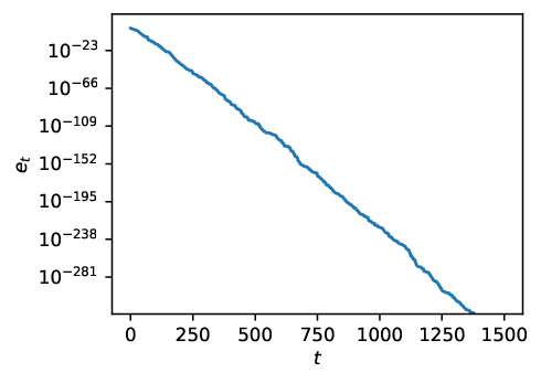
Figure 1(b) and (c) reveals an essential difference between the ACR and CR. The sequence $\{CR_{t};t\in\mathbb{Z}^{+}\}$ oscillates, but the sequence $\{ACR_{t};t\in\mathbb{Z}^{+}\}$ is more stable. In practice, the calculation of $ACR_{t}$ is easy and it results in an exact erro expression $e(t)=e_{0}(ACR_{t})^{t}$. However, it is difficult to obtain the same expression from $CR_{t}$.

In the above ACR definition, the optimal fitness value $f^{*}$ is required. In case of $f^{*}$ unknown, an alternative average convergence rate is defined by [13].

where $\tau$ is an appropriate and user-defined time interval. In computer simulation, it is necessary to set $\tau$ to a large value. This reduces noise in calculating $ACR^{\dagger}_{t}$. It should be mentioned that the alternative ACR is not defined for $t<\tau$.

Using the ACR or alternative ACR, it is convenient to quantify and visualize the convergence speed of EAs. Let us show this claim through computer simulation.

For the purpose of illustration, consider (1+1) evolutionary programming (Algorithm 2) for minimizing the 2-d sphere function as an example. The sphere function is a unimodal function which is often used as a benchmark in EAs [28].

The minimal point to this function is $\mathbf{x}^{*}=(0,0)$ with $f^{*}=0$.

Evolutionary programming (EP) is a type of EAs which employs mutation and selection but without recombination. (1+1) EP is equivalent to (1+1) evolutionary strategies (ES) without crossover. However, a population-based ES employs a recommendation operator [29].

A child $\mathbf{y}$ is generated by Gaussian mutation $\mathbf{y}=\mathbf{x}+\mathbf{z}$, where $\mathbf{z}=(z_{1},\cdots,z_{d})$ obeys the Gaussian probability distribution $z_{i}\sim\mathcal{N}(0,\sigma_{i})$. Two variants of Gaussian mutation are chosen with different settings of $\boldsymbol{\sigma}=(\sigma_{1},\cdots,\sigma_{d})$.

• 1.

  Invariant Gaussian mutation: $\boldsymbol{\sigma}$ is set to constants, that is, for any $i$, $\sigma_{i}$ is a constant. The (1+1) EP using invariant Gaussian mutation is called the (1+1) invariant EP.

• 2.

  Adaptive Gaussian mutation: $\boldsymbol{\sigma}$ varies as $\mathbf{x}$, that is, $\boldsymbol{\sigma}$ is a function of $\mathbf{x}$. The (1+1) EP using adaptive Gaussian mutation is called the (1+1) adaptive EP.

In computer simulation, set $\sigma_{i}=1$ in the (1+1) invariant EP and $\sigma_{i}=|x|_{i}$ in the (1+1) adaptive EP. The adaption is based on commonsense in the design of EAs: as $\mathbf{x}$ is close to the optimal solution $0$, $\boldsymbol{\sigma}$ is set to a small value. This is equivalent to the practical strategy: as $t$ increases, $\mathbf{x}_{t}$ is close to the optimal solution, then $\boldsymbol{\sigma}$ is reduced. $\mathbf{x}_{0}$ is randomly generated in $[-20,20]^{2}$. Each algorithm runs $1,000$ times independently and $f_{t}$ is the average over the 1,000 runs. The maximum number of generations is $300$. The time interval $\tau$ for calculating the alternative ACR is chosen to be $50$.

The first experiment is to compare the ACR and alternative ACR of the adaptive EP on the sphere function. Trend plots of the ACR and alternative ACR are illustrated in Figure 2. Figure 2(a) shows that the ACR of the adaptive EP increases to a positive, while Figure 2(b) depicts similar tends of the alternative ACR. But $ACR^{\dagger}_{t}$ suffers a little bigger noise than $ACR_{t}$ due to the introduction of the $\tau$-th order difference.

The second experiment is to compare the ACR and alternative ACR of the invariant EP on the sphere function. Trend plots of the ACR and alternative ACR are illustrated in Figure 3. Figure 3(a) shows that the ACR decreases as time, while Figure 3(b) depicts a similar tend for the alternative ACR.

The results reveal that the adaptive EP converges faster than the invariant EP. For the adaptive EP, its ACR and alternative ACR both tend to a positive constant between 0.38 to 0.4. In general, an ACR is called linear if it tends towards a positive. But for the invariant EP, its ACR and alternative ACR decreases to a smaller constant and eventually towards 0. In general, an ACR is called sublinear if it converges to 0.

The ACR is more stable than the CR in numerical calculation. Let us show the claim through computer simulation.

The first experiment is to compare the ACR and CR of the (1+1) adaptive EP on the sphere function. Experimental setting is the same as that in the previous subsection. Figure 4 illustrates trend plots of the ACR and CR. The CR fluctuates greatly between 0 and 1. It is impossible to quantify the convergence speed using the CR. But the ACR clearly converges to a positive constant around 0.38.

The second experiment is to compare the ACR and CR of the (1+1) invariant EP on the sphere function. Experimental setting is the same as that in the previous subsection. Figure 5 illustrates trend plots of the ACR and CR. The figure shows that the CR converges to 1 and the ACR to 0. The difference is caused by the normalization in the ACR to ensure the lower ACR, the slower convergence. Figure 5(b) reveals that the convergence speed of the (1+1) invariant EP eventually decreases to 0.

The experimental results confirm that the numerical calculation of the ACR is more stable than the CR.

The ACR of EAs will decrease as the decision space dimension increases. Let us verify this claim through computer simulation.

For the sake of illustration, consider a (1+1) random univariate search method (RUS), described in Algorithm 3, as an example. This algorithm can be regarded as random local search in continuous optimization because both make a random one-dimensional search at each generation. The RUS using adaptive Gaussian mutation is called the adaptive RUS in short.

Two test functions are used in computer simulation. The functions are inspired from the OneMax function and deceptive function in pseudo-Boolean function optimization. The OneMax function is the easiest to a (1+1) elitist EA and the deceptive function is the hardest [30]. A variant OneMax function in continuous optimization is defined by

where $\mathbf{x}^{*}=(0,\cdots,0)$ and $f^{*}=d$.

A deceptive function in continuous optimization is defined by

The global optimum is $\mathbf{x}^{*}=(0,\cdots,0)$ and $f^{*}=d+1$. The basin of attraction of $\mathbf{x}^{*}$ is $\{\mathbf{x}\mid\sum_{i=1}^{d}x_{i}\leq 1/2\}$. The deceptive function (8) has a local optimum at $(1,\cdots,1)$.

In computer simulation, set $\sigma_{j}=x_{j}$ for the selected index $j$ in the adaptive RUS. $\mathbf{x}_{0}$ is chosen from $[0,1]^{d}$ at random. The algorithm runs $2,000$ times independently on each test function. $f_{t}$ is the average over the 2,000 run. The maximum number of generations is $500$.

The experiments is to compare the ACR between the variant OneMax function and deceptive function. Trend plots of the ACR are illustrated in Figure 6. Figure 6(a) shows that the ACR on the variant OneMax function converges to some positive constants over generations for $d=1,3,5$. But Figure 6(b) depicts the ACR on the deceptive function decreases quickly as the dimension $d$ increases.

The experimental results demonstrate that the ACR decreases as the dimension increases. For an easy function like the OneMax function, the ACR decreases slowly as the dimension. In theory, it is expected that the ACR is larger than the reciprocal of a polynomial function of $d$. But for a hard function like the deceptive function, the ACR decreases quickly as the dimension increases. In theory, it is expected that the ACR is less than the reciprocal of an exponential function of $d$.

Computer simulation in Section 3.3 shows an advantage of the ACR over the CR, that is, when a CR sequence oscillates, the ACR sequence is still stable. This subsection explains this difference.

The terms of linear, sub-linear or super-linear convergence has been used in describing the convergence speed of an iterative sequence. In EAs, a sequence $\{CR_{t},t\in\mathbb{Z}^{+}\}$ converges linearly if $\lim_{t\to+\infty}CR_{t}<1$ or converges sublinearly if $\lim_{t\to+\infty}CR_{t}=1$. Similarly, a sequence $\{ACR_{t},t\in\mathbb{Z}^{+}\}$ converges linearly if $\lim_{t\to+\infty}ACR_{t}>0$ or converges sublinearly if $\lim_{t\to+\infty}ACR_{t}=0$.

From the definition

the linear convergence of the ACR can be derived from the linear convergence of the CR. But the inverse does not hold. This is the main advantage of the ACR over the CR. Let us verify the claim using an example.

Let us consider an example which is (1+1) EP (Algorithm 4) combining Cauchy and Gaussian mutation together. Because Cauchy and Gaussian mutation operators have different probability density functions, combination of them could result in faster convergence [31, 32, 33, 34].

Two mutation operators are alternately used in this (1+1) EP, that is, Cauchy mutation is applied when $t$ is an odd number and Gaussian mutation is applied when $t$ is an even number. Thus, $z_{t}$ obeys Cauchy or Gaussian probability distribution, probability density functions of which are $p_{c}=\frac{1}{\pi(1+x^{2})}$ and $p_{g}=\frac{1}{\sqrt{2\pi}}e^{-\frac{x^{2}}{2}}$, respectively.

The (1+1) EP is used to minimize a JUMP function which is a typical multi-modal problem. This function is similar to the JUMP function in pseudo-Boolean optimization [35]. The the optimal solution set is $\{x;|x|<1\}$.

For the sake of analysis, assume that the initial point ${x}_{0}=2$. After $t(t\geq 1)$ iterations, ${x}_{t}$ either jump to the flat $\{|x|<1\}$ or stay at $|x|=2$. Thus, the reduction rate of expected error is (without loss of generality, let $x_{t}=2$ or $|x_{t}|<1$)

Moreover, the conditional expectation of error change is for Cauchy mutation,

and for Gaussian mutation,

where $\Phi(\cdot)$ is cumulative distribution function (CDF) of the standard Gaussian distribution. From (13), (14) and (15) we know that for any integer $k\geq 1$

and

Since $C_{a}\neq C_{b}$, the sequence $\{CR_{t}\}$ oscillates and does not converge.

However, from

we get $ACR_{t}\to 1-(C_{a}C_{b})^{1/2}$ as $t\to+\infty$, that is, the sequence $\{ACR_{t}\}$ is convergent.

This example shows that the CR sequence could oscillate and not converge in some adaptive EAs. However, the ACR sequence converges thanks to the average of the CR for consecutive generations.

In order to make a theoretical analysis, EAs under investigation are assumed to satisfy several conditions.

1. 1.

   (Supermartingale). The expected approximation error does not increase. For any non-optimal $X_{0}$ and any $t$,

   $$\mathbb{E}[e(X_{t+1})\mid X_{0},\cdots,X_{t}]\leq e(X_{t}).$$

   (16)

   The sequence $\{e_{t};t=0,1,\cdots\}$ is a monotonically decreasing function of $t$. This condition is different from elitism in EAs which requires $e(X_{t+1})\leq e(X_{t})$. A direct consequence from this condition is $ACR_{t}\in[0,1]$.

2. 2.

   (Markov chain). The state of $X_{t+1}$ depends on $X_{t}$ only. For any $X_{0}$ and any $t$, the transition probability

   $$\Pr(X_{t+1}\mid X_{0},\cdots,X_{t})=\Pr(X_{t+1}\mid X_{t}).$$

   (17)

3. 3.

   (Stochastic algorithm). Starting from any non-optimal $X_{0}$, for any $t$, it holds

   $$\Pr(X_{t}\cap X^{*})<1,\quad(\mbox{then }e_{t}>0).$$

   (18)

   If $\Pr(X_{t}\cap X^{*})=1$, an EA reaches the optimal set at the $t^{th}$ generation with probability 1. It degenerates to a deterministic-like algorithm.

4. 4.

   (Normal reduction). The reduction rate of the approximation error satisfies

   $\displaystyle\lim_{t\to+\infty}\left(\frac{e_{t}}{e_{t-1}}\right)^{1/t}=1.$

   (19)

   The condition holds for normal EAs. If this condition doesn’t hold, $\lim_{t\to+\infty}(e_{t}/e_{t-1})^{1/t}<c<1$, then for a large $t$, $e_{t}/e_{t-1}<c^{t}$. For example, let $c=0.9$ and $t=1000$, we have $e_{1000}<1.75\times 10^{-46}e_{999}$. This rapid reduction rate is unpractical in normal EAs.

Many EAs satisfy the above four conditions. By default, they are always assumed to be true in the theoretical study in this paper.

Markov chains associated with EAs can be classified into homogeneous and inhomogeneous, depending on whether genetic operators (mutation, crossover and selection) change over time [8]. This paper focuses on two types of EAs which are modeled by homogeneous Markov chains as below.

1. 1.

   The population sequence $\{X_{t};t=0,1,\cdots\}$ is a homogeneous Markov chain, that is, for any $t$, any $X$ and any subset $\mathcal{A}\subset\mathcal{S}$, the transition probability

   $$\Pr(X_{t+1}\in\mathcal{A}\mid X_{t}=X)=P(X;\mathcal{A}).$$

   (20)

   Transition probabilities do not change over time.

2. 2.

   A population subsequence $\{X_{\kappa t},t=0,1,\cdots\}$ (where $\kappa>1$) is a homogeneous Markov chain. Transition probabilities follow a periodic change over generations. Let $Y_{t}=X_{\kappa t}$.

   		$\displaystyle\Pr(Y_{t+1}\in\mathcal{A}\mid Y_{t}=X)=P^{(\kappa)}(X;\mathcal{A}),$		(21)
   		$\displaystyle\mbox{but }\Pr(X_{t+1}\in\mathcal{A}\mid X_{t}=X)\neq\Pr(X_{t+2}\in\mathcal{A}\mid X_{t+1}=X).$		(22)

   The original population sequence $\{X_{t};t=0,1,\cdots\}$ is an inhomogeneous Markov chain.

The current paper will not discuss other types of EAs whose genetic operators change over time. Their analysis needs further understanding of inhomogeneous genetic operators and advanced tools from inhomogeneous Markov chains or stochastic processes. This topic is left for future research.

Computer simulation in Section 3.2 demonstrates different trend plots of the ACR for the (1+1) invariant EP and (1+1) adaptive EP. The ACR sequence has different limit properties. In practice, it is required that $e_{t}$ converges to $0$, however this does not imply that $ACR_{t}$ will converge as $t\to\infty$. Thus, the limit superior and limit inferior [36] of the sequence $\{ACR_{t}\}$, defined as (23) and (24) respectively, are introduced to describe the limit property.

where $\inf$ is the abbreviation of mathematical infimum and $\sup$ the abbreviation of supremum. An example of the limit superior and inferior is illustrated in Figure 7. Consider the sequence $R_{t}=0.1\cos(t)\times(\exp(-0.1t)+0.1)$ where $t=0,1,2,\cdots$. Although the sequence does not converge, its limit superior ($-0.1$) and inferior ($-0.1$) still exist.

Existing theoretical results [37, 38, 10] show that the convergence rate of EAs in continuous optimization is up to linear. Similarly, the ACR of EAs can be classified into two categories via its limit property.

• 1.

  The ACR is linear, if its limit inferior is a positive, that is, $\varliminf_{t\to+\infty}ACR_{t}=C>0$. In this case, the approximation error reduces geometrically fast to 0. For example, the ACR in Figure 2 is linear.

• 2.

  The ACR is sublinear, if it asymptotically reduces to zero as $t\to+\infty$, that is, $\lim_{t\to+\infty}ACR_{t}=0$. In this case the approximation error converges slowly to 0. For example, the ACR in Figure 3 is sublinear.

The ACR can be estimated using one-step transition or multi-step probability transition. Given an error sequence $\{e_{t},t=0,1,\cdots\}$, the one-step error change at the $t^{th}$ generation is $\Delta e_{t}:=e_{t}-e_{t+1}.$ It is similar to the quality gain [20] but the latter is defined on the fitness mean of individuals in a population $\bar{f}_{t}$ rather than the error mean $e_{t}$. The rate of one-step error change is ${\Delta e_{t}}/{e_{t}}$. Given a positive integer $\kappa$, the $\kappa$-step error change at the $t^{th}$ generation is $\Delta^{(\kappa)}e_{t}:=e_{t}-e_{t+\kappa}.$ The rate of $\kappa$-step error change is ${\Delta^{(\kappa)}e_{t}}/{e_{t}}$.

To derive the linear ACR sequence, Condition (25) requires the rate of $\kappa$-step error change larger than a positive. This condition is weaker than the rate of the one-step error change larger than zero. But to derive the sublinear convergence of the ACR sequence, Condition (26) requires the rate of one-step error change to converge to 0.

Computation simulation in Section 3.2 shows the ACR and alternative ACR have similar behaviors. There is a link between the ACR and alternative ACR. Under some conditions, their limits are identical.

The above theorem proves that the limit of $ACR_{t}$ is identical to the limit of $ACR^{\dagger}_{t}$. If the $f^{*}$ value is unknown, $ACR^{\dagger}_{t}$ can be used as a replacement of $ACR_{t}$.

In Section 3.2, it is observed that the ACR of invariant EP tends to zero, while the ACR of adaptive EP tends to a positive constant. This section analyzes general EP (Algorithm 5) using landscape-invariant or landscape-adaptive mutation. We only consider genetic operators which are unchanged over time or have periodic change. So, the population sequence or a subsequence is a homogeneous Markov chain.

Mutation $Y=X+Z$ can be characterized by probability transition. Given a population ${X}\in\mathcal{S}$ and a subset $\mathcal{A}\subset\mathcal{S}$, the transition probability kernel $P_{g}({X};\mathcal{A})$ [39] is defined as

where $p_{g}({X};Y)$ is the probability density function depicting the mutation transition from ${X}$ to ${Y}$. Furthermore, the $\kappa$-step kernel is defined as

In this paper, we assume it is continuous and bounded.

Generally, mutation operators can be classified into two categories.

• 1.

  Landscape-invariant mutation: mutation $Y=X+Z$ is called landscape-invariant if $Z$ is a random variable vector whose joint probability density function $p_{g}({0};{Z})$ is independent on $X$. For simplicity, denote $p_{g}({0};{Z})$ as $p_{z}(Z)$. EP using invariant mutation is named invariant EP. For example, the Gaussian mutation using invariant $\sigma$ in Section 3.2 belongs to invariant mutation.

• 2.

  Landscape-adaptive mutation: if the probability density function of $Z$ varies on $X$, mutation $Y=X+Z$ is called landscape-adaptive. EP using adaptive mutation is named adaptive EP. For example, the Gaussian mutation using adaptive $\sigma$ in Section 3.2 is adaptive mutation.

References

- [1] J. He, X. Yao, Drift analysis and average time complexity of evolutionary algorithms, Artificial Intelligence 127 (1) (2001) 57–85.
- [2] Y. Chen, X. Zou, J. He, Drift conditions for estimating the first hitting times of evolutionary algorithm, International Journal of Computer Mathematics 88 (1) (2011) 37–50.
- [3] A. Agapie, M. Agapie, G. Rudolph, G. Zbaganu, Convergence of evolutionary algorithms on the -dimensional continuous space., IEEE Transactions on Cybernetics 43 (5) (2013) 1462–1472.
- [4] H. Huang, J. Su, Y. Zhang, Z. Hao, An experimental method to estimate running time of evolutionary algorithms for continuous optimization, IEEE Transactions on Evolutionary Computation 24 (2) (2020) 275–289.
- [5] G. Rudolph, Local convergence rates of simple evolutionary algorithms with Cauchy mutations, IEEE Transactions on Evolutionary Computation 1 (4) (1997) 249–258.
- [6] G. Rudolph, et al., Convergence rates of evolutionary algorithms for a class of convex objective functions, Control and Cybernetics 26 (1997) 375–390.
- [7] J. He, L. Kang, On the convergence rate of genetic algorithms, Theoretical Computer Science 229 (1-2) (1999) 23–39.
- [8] J. He, X. Yu, Conditions for the convergence of evolutionary algorithms, Journal of Systems Architecture 47 (7) (2001) 601–612.
- [9] A. Auger, Convergence results for the (1, )-sa-es using the theory of -irreducible markov chains, Theoretical Computer Science 334 (1-3) (2005) 35–69.
- [10] A. Auger, N. Hansen, Linear convergence of comparison-based step-size adaptive randomized search via stability of markov chains, SIAM Journal on Optimization 26 (3) (2016) 1589–1624.
- [11] J. He, Y. Zhou, G. Lin, An initial error analysis for evolutionary algorithms, in: Proceedings of the Genetic and Evolutionary Computation Conference Companion, ACM, 2017, pp. 317–318.
- [12] D. Tarłowski, On geometric convergence rate of markov search towards the fat target, Operations Research Letters 46 (1) (2018) 33–36.
- [13] J. He, G. Lin, Average convergence rate of evolutionary algorithms, IEEE Transactions on Evolutionary Computation 20 (2) (2016) 316–321.
- [14] H. Dong, T. Li, R. Ding, J. Sun, A novel hybrid genetic algorithm with granular information for feature selection and optimization, Applied Soft Computing 65 (2018) 33–46.
- [15] T. Dhivyaprabha, P. Subashini, M. Krishnaveni, Synergistic fibroblast optimization: a novel nature-inspired computing algorithm, Frontiers of Information Technology & Electronic Engineering 19 (7) (2018) 815–833.
- [16] D. Janiga, R. Czarnota, J. Stopa, P. Wojnarowski, Self-adapt reservoir clusterization method to enhance robustness of well placement optimization, Journal of Petroleum Science and Engineering 173 (2019) 37–52.
- [17] T. Li, H. Dong, J. Sun, Binary differential evolution based on individual entropy for feature subset optimization, IEEE access 7 (2019) 24109–24121.
- [18] L. Ding, L. Kang, Convergence rates for a class of evolutionary algorithms with elitist strategy, Acta Mathematica Scientia 21 (4) (2001) 531–540.
- [19] M. A. Semenov, D. A. Terkel, Analysis of convergence of an evolutionary algorithm with self-adaptation using a stochastic lyapunov function, Evolutionary Computation 11 (4) (2003) 363–379.
- [20] H.-G. Beyer, The theory of evolution strategies, Springer Science & Business Media, 2013.
- [21] H.-G. Beyer, A. Melkozerov, The dynamics of self-adaptive multirecombinant evolution strategies on the general ellipsoid model, IEEE Transactions on Evolutionary Computation 18 (5) (2014) 764–778.
- [22] H.-G. Beyer, M. Hellwig, The dynamics of cumulative step size adaptation on the ellipsoid model, Evolutionary computation 24 (1) (2016) 25–57.
- [23] Y. Akimoto, A. Auger, N. Hansen, Quality gain analysis of the weighted recombination evolution strategy on general convex quadratic functions, in: Proceedings of the 14th ACM/SIGEVO Conference on Foundations of Genetic Algorithms, ACM, 2017, pp. 111–126.
- [24] A. Auger, N. Hansen, Reconsidering the progress rate theory for evolution strategies in finite dimensions, in: Proceedings of the 8th annual conference on Genetic and evolutionary computation, ACM, 2006, pp. 445–452.
- [25] A. Auger, N. Hansen, Theory of evolution strategies: a new perspective, in: Theory of Randomized Search Heuristics: Foundations and Recent Developments, World Scientific, 2011, pp. 289–325.
- [26] M. Jebalia, A. Auger, N. Hansen, Log-linear convergence and divergence of the scale-invariant (1+ 1)-es in noisy environments, Algorithmica 59 (3) (2011) 425–460.
- [27] R. Varga, Matrix Iterative Analysis, Springer, 2009.
- [28] B.-Y. Qu, J. Liang, Z. Wang, Q. Chen, P. N. Suganthan, Novel benchmark functions for continuous multimodal optimization with comparative results, Swarm and Evolutionary Computation 26 (2016) 23–34.
- [29] T. Bäck, G. Rudolph, H.-P. Schwefel, Evolutionary programming and evolution strategies: Similarities and differences, in: D. B. Fogel, W. Atmar (Eds.), Proceedings of the Second Annual Conference on Evolutionary Programming, Evolutionary Programming Society, San Diego, CA, 1993, pp. 11–22.
- [30] J. He, T. Chen, X. Yao, On the easiest and hardest fitness functions, IEEE Transactions on Evolutionary Computation 19 (2) (2015) 295–305.
- [31] K. Chellapilla, Combining mutation operators in evolutionary programming, IEEE transactions on Evolutionary Computation 2 (3) (1998) 91–96.
- [32] X. Yao, Y. Liu, G. Lin, Evolutionary programming made faster, IEEE Transactions on Evolutionary computation 3 (2) (1999) 82–102.
- [33] H. Dong, J. He, H. Huang, W. Hou, Evolutionary programming using a mixed mutation strategy, Information Sciences 177 (1) (2007) 312–327.
- [34] R. Mallipeddi, S. Mallipeddi, P. N. Suganthan, Ensemble strategies with adaptive evolutionary programming, Information Sciences 180 (9) (2010) 1571–1581.
- [35] T. Jansen, C. Zarges, Performance analysis of randomised search heuristics operating with a fixed budget, Theoretical Computer Science 545 (2014) 39–58.
- [36] J. Snow, K. Weller, Exploratory Examples for Real Analysis, Mathematical Association of America, 2003.
- [37] O. Teytaud, S. Gelly, General lower bounds for evolutionary algorithms, in: Parallel Problem Solving from Nature-PPSN IX, Springer, 2006, pp. 21–31.
- [38] H.-G. Beyer, Convergence analysis of evolutionary algorithms that are based on the paradigm of information geometry, Evolutionary Computation 22 (4) (2014) 679–709.
- [39] S. Meyn, R. Tweedie, Markov chains and stochastic stability, Springer Verlag, 1993.
- [40] D. Tarłowski, On the convergence rate issues of general markov search for global minimum, Journal of Global Optimization 69 (4) (2017) 869–888.