Monitoring the shape of weather, soundscapes, and dynamical systems: a new statistic for dimension-driven data analysis on large data sets

As high-dimensional data becomes more and more plentiful, dimensionality-reduction algorithms become an increasingly important tool for any researcher seeking to extract meaningful information from their data. Indeed, it is not unusual to find that data collected in an $n$-dimensional space is intrinsically only $k$-dimensional, where $k\ll n$. A good dimensionality-reduction algorithm will find a map which takes the data from $\mathbb{R}^{n}$ to $\mathbb{R}^{k^{\prime}}$ (for some $k^{\prime}$ close to $k$) while preserving fundamental properties such as the distances between data points. This process is fundamental since data in low-dimensional space is often computationally easier to store and manipulate, and hence a wider array of algorithms are available for data analytics. Furthermore, the process of reduction often coincides with the production of a more appropriate representation of the data, making many data analytics algorithms more successful as a result of a meaningful feature space.

By systematically studying how well a data set $D$ in $\mathbb{R}^{n}$ can be projected to $\mathbb{R}^{m}$ for $m<n$, as $m$ varies, we can begin to uncover basic geometric properties of $D$ (such as the intrinsic dimension of an underlying manifold on which $D$ approximately sits). In this paper we will explore this idea in the context of secant-based dimensionality reduction algorithms. These are a family of dimensionality-reduction algorithms that use the secant set $S$ of $D$ to find projections that best preserve distances between points. As a consequence of producing these projections, the algorithms also return a statistic which we call the $\kappa$-profile. We will focus on $\kappa$-profiles obtained from SAP and HSAP dimensionality-reduction algorithms [1, 2].

The problem of calculating the dimension of a data set has been addressed from various perspectives. The classical approach to estimating dimension is to use a linear method such as principal component analysis (PCA). However, such methods do not capture the dimension of non-linear data well. Other methods that do not assume linearity have also been proposed, see for example [3, 4, 5, 6, 7, 8, 9].

Though it is related to dimension, the $\kappa$-profile often carries more information. In particular, one may observe gradual transitions in $\kappa,$ whereas an estimate of the intrinsic dimension will by nature either remain constant or have a sudden jump discontinuity. The $\kappa$-profile also gives information about how well the data fits into many different reduced dimensions simultaneously. This is useful for studying real-world data that almost never conforms precisely to a manifold.

The $\kappa$-profile can be used not only for analysis of a static data set, but also for settings such as time series analysis and anomaly detection. In particular, the sensitivity of the $\kappa$-profile to changes in the geometry of a data set makes it a prime candidate as an indicator of fundamental changes in the behavior of an underlying system as a function of either time or a set of parameters. A useful transformation that helps to reveal structure underlying a time series is achieved through a time-delay embedding. In fact, by considering our data via a time-delay embedding, the $\kappa$-profile can in some cases also give indication of the dimension of the underlying dynamics from which the data is drawn.

Estimating the $\kappa$-profile from a data set is relatively easy and requires very few assumptions about the data. It is thus a useful statistic, particularly in cases in which domain-specific tools are limited.

This paper is organized as follows. In Section II we review the mathematical concept of dimension of a dataset, secant-based dimensionality reduction algorithms, and formally define the $\kappa$-profile. We also include a brief review of geodesic distance on a Grassmann manifold in order to provide context for comparison between dimensionality-reduction related to the $\kappa$-profile and dimensionality-reduction via principal component analysis. In Section III we discuss ways to format a collection of time-parametrized data sets prior to calculating the $\kappa$-profile and provide mathematical justification for this framework. In Section IV we discuss a synthetic example where the dimension of the data, the solution set of a well-known partial differential equation, is already approximately known. In V and VI we calculate the $\kappa$-profile on weather data and ambient noise data respectively.

We begin by reviewing mathematical prerequisites.

The $\kappa$-profile can also provide information about the dynamics underlying data that is changing over time. Suppose that we are given a collection of data sets $\{D_{t}\}$ in $\mathbb{R}^{n}$ parametrized by time parameter $t\in\mathbb{Z}_{\geq 0}$, as well as a collection of bijective maps $f_{t}:D_{t}\rightarrow D_{t+1}$. Then we can identify points in $D_{t}$ and $D_{t+1}$, so that $f_{t}(x)\in D_{t+1}$ is the same point as $x\in D_{t}$, but one time step later.

Given such a collection $\{D_{t}\}$ there are various ways of calculating the $\kappa$-profile depending on how we structure the input data. One approach is to create a $\kappa$-profile for each $D_{t}$ independently. That is, the secant set we apply our dimensionality reduction algorithm to is precisely the secant set of points $D_{t}\subset\mathbb{R}^{n}$ for each $t\in\mathbb{Z}_{\geq 0}$. This captures geometric properties of $\{D_{t}\}$ as $t$ changes. When we also want a single $\kappa$-profile to capture temporal changes in the data, an alternative approach is to construct a new sequence of data sets $\{D_{t}^{(\ell)}\}$ such that:

where the brackets indicate vector concatenation. This type of construction is often known as a time-delay embedding.

Motivation for this approach is given by Takens theorem [17]. Given a discrete dynamical system where the state space is an $m$-dimensional compact, smooth manifold $M$, evolution of the system can be defined as a smooth map $f:M\rightarrow M$. Suppose that we only have access to a single smooth measurement function $\varphi:M\rightarrow\mathbb{R}$. Takens theorem says that under suitably general conditions, we can construct a diffeomorphic copy of the manifold $M$ in $\mathbb{R}^{k}$ via a length $k\geq 2m+1$ time-delay embedding of $\varphi$ with respect to $f$, i.e. we define the embedding by sending $x$ to $[\varphi(x),f(\varphi(x)),\dots,f^{k}(\varphi(x))]$.

Hence when considering the problem of monitoring a large collection of data that is changing over time, it is useful to use time-delay embeddings so that we can not only monitor the current geometry of the data, but also changes in the dynamics of the data. In Section V, we provide an example in which we use this framework to calculate $\kappa$-profiles for two weather data sets over time.

Of course in the real world, we rarely know the dimension of the manifold $M$, as we generally only have access to some of the variables defining the dynamics of the system. It is an important problem therefore to estimate the value $2m+1$, or the shortest time-delay embedding that will fully capture the dynamics. Algorithms which address this problem include false nearest neighbors [18] and saturation methods [19]. In the spirit of the latter, the $\kappa$-profile should provide a new tool to approach this problem. Specifically, one should be able to estimate the value $2m+1$ by calculating the $\kappa$-profile for a data set $D_{t}^{(i)}$ for increasingly large $i$. When the embedding dimension is reached, change in the $\kappa$-profile for increasing $i$ should cease. We intend to explore this idea in future research.

The Kuramoto-Sivashinsky (KS) equation [20] in one spatial dimension is the partial differential equation

where $v$ is a positive constant, $u:\mathbb{R}\times\mathbb{R}_{\geq 0}\rightarrow\mathbb{R}$ is a function that satisfies an $L$-periodic initial condition $u(x+L,0)=u(x,0)$, and each subscript on $u$ denotes a partial derivative with respect to that subscript. The KS equation was originally derived by Kuramoto for modeling the Belouz-Zabotinskii reaction [21]. It was also developed by Sivashinsky to model thermal diffusive instabilities in laminar flame fronts [22]. For $u(x,0)$ satisfying the initial condition, it has been proven that a unique solution exists and it is bounded. These solutions have the interesting characteristic that while they have coherent spatial structure, they exhibit temporal chaos. Furthermore, for different initial conditions and periodicity values $L$, the solution manifold has varying dimension. This makes data collected from the KS equation ideal for studying algorithms whose output should capture the dimension of a data set or related statistics.

Following [20], the version of the KS equation that we use to generate data is

where the periodicity has been set at $2\pi$, $v=4$, and a bifurcation parameter $\alpha$ has been introduced. The stable solution manifolds for various values of $\alpha$ were described via numerical experiment in [20].

We now consider some examples with varying values of $\alpha$ and hence dimension. In each case, we generate a data set from the solution manifold consisting of 10,000 points in $\mathbb{R}^{32}.$ In several of these examples, we also provide a comparison with the PCA approach to dimensionality reduction for context.

Let us begin with $\alpha=19.$ In this case, the authors of [20] note that the solution is a periodic orbit. In Figure 1, we show the $\kappa$-profile for projection dimensions 1 to 20 for this value of $\alpha$ as well as several others. By heuristic, if the value of $\kappa$ is above 0.2, we consider the embedding to be good. Thus in this case, we can reasonably embed the data in $\mathbb{R}^{1}.$ It is worth noting as well that the projection into $\mathbb{R}^{7}$ is nearly isometric on the normalized secant set since the value of $\kappa$ is very close to one.

For comparison, consider the singular values of the data set, shown in Figure 2. In this example and throughout the paper, the data is not mean-subtracted. From the singular values for $\alpha=19$, we infer similar information to that contained in the $\kappa$-profile: the data can be projected into $\mathbb{R}^{1}$ or $\mathbb{R}^{2}$ without much loss of information. The two vectors that form a basis for the 2-dimensional subspace into which the data is projected for PCA and SAP are shown in Figure 3; while they capture similar information, they provide distinct projections. Note that the geodesic distance between the subspaces is approximately 0.6. For each embedding dimension, we consider the geodesic distance between the subspace that defines the PCA projection and that of the SAP projection; see Figure 4. Note that the subspaces are somewhat distinct for projections to $\mathbb{R}^{m}$ with $m<7.$

For a different choice of the parameter $\alpha,$ we see distinctly different behavior. For example, consider $\alpha=54.$ The $\kappa$-profile for this $\alpha$ is shown in Figure 1. In this example, we get a good projection of the data starting at dimension 4. For comparison, consider the singular values of the data shown in Figure 2. Here, too, we see a change in behavior at dimension 4. However, the dimension estimate inferred from the singular values is not obvious - one could argue that the energy or variance in the data isn’t essentially captured until some dimension between 10 and 15. Thus, the added information from the $\kappa$-profile is valuable. In this case, we see that we have a near isometry on the set of normalized secants when projecting into $\mathbb{R}^{8}.$ In [20], this choice of $\alpha$ is stated to coincide with oscillatory and/or chaotic orbits.

As a final example from the KS equation data, we consider $\alpha=117.5,$ which produces chaotic orbits [20]. We show the $\kappa$-profile in Figure 1 and the singular values in Figure 2. Here we see that the more complex behavior of the solution set is reflected in the $\kappa$-profile: a good projection arises at dimension 6, and the $\kappa$ values increase more gradually than in the previous two examples with $\alpha=19$ and $\alpha=54.$ The jump between dimensions 6 and 7 in the singular values mirrors the information in the $\kappa$-profile. As before, the dimension estimate from the singular values is not obvious, so the $\kappa$-profile stands to provide meaningful additional context.

We include in Figure 4 a plot of the geodesic distance between the PCA and SAP projection subspace bases for dimensions 1 to 20 for all three choices of parameter $\alpha.$ Note that the PCA and SAP projections consistently differ in the low to intermediate dimensions.

Statistics arising from measurements of the Earth’s weather is one of the most fertile sources of big data available. In this section we provide an example of how large-scale regional weather patterns are reflected in the $\kappa$-profile of weather data sets.

We obtained historical weather model data from the National Center for Environmental Prediction (NCEP) Climate Forecast System (CFS), version 2 [23]. We took two rectangular grids, with data points at each $.5^{\circ}$ of latitude/longitude:

• •

  The first is in the Western Atlantic ($20-33^{\circ}$N, $44-69^{\circ}$W), northeast of the Caribbean and in the path of Atlantic hurricane activity. The time frame for this data set is from April 1st 2014, to October 1st 2014 with measurements every 6 hours.

• •

  The second is located in the Western Pacific ($18-26^{\circ}$N, $123-132^{\circ}$E) east of Taiwan in the line of some of the Pacific typhoon activity. The time frame for this data set is from July 1st, 2015 to December 1st, 2015 with measurements every 6 hours.

The data contains $9$ weather variables at each grid point which include pressure, wind speed, air temperature, precipitation rate, etc. We consider points of these data sets to be the weather variables at a given grid location so that (before the time-delay embedding) the data sets consists of points in $\mathbb{R}^{9}$. We used a $19$ step time-delay embedding in order to construct new data sets $\{D_{A,t}\}$ (corresponding to the data from the Western Atlantic) and $\{D_{P,t}\}$ (corresponding to the data from the Western Pacific) from which we produced the $\kappa$-profiles that we analyze below. Note that for each time step $t$, corresponding to a 171 hour time window, $D_{A,t}$ and $D_{P,t}$ are sets of points in $\mathbb{R}^{171}$. As described in Section III, one of the reasons for using a time-delay embedding is to capture the temporal dynamics of the entire weather system in this area.

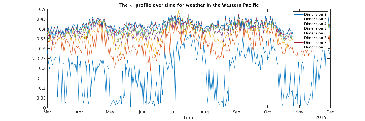
In Figures 5 and 6 we provide $\kappa$-profiles for $\{D_{A,t}\}$ and $\{D_{P,t}\}$. We see that in both cases elements of $\{D_{A,t}\}$ and $\{D_{P,t}\}$ fluctuate between being 2 and 3 dimensional. This is further supported by examining projections of the data, obtained by the SAP algorithm (see Figures 7 and 8 for example). Rough comparisons of these figures with the record of storms (hurricanes and typhoons respectively) suggests that in general the $\kappa$-values decrease as a storm approaches (indicating an increase in the dimension of the data), and increase again when no major weather events are occurring. We hypothesize for example that the drop in $\kappa$-values in Figure 5 in late-June/early-July is related to Hurricane Arthur which passed by the grid near this time (taking into account the time-delay embedding). It also seems likely that the drop in $\kappa$ values in mid-August is related to Hurricane Cristobal.

In Figures 7 and 8 we project points from two elements of the collection $\{D_{A,t}\}$, from $\mathbb{R}^{171}$ into $\mathbb{R}^{3}$, using projections obtained from the SAP algorithm. Figure 7 corresponds to June 30th at 12:00pm, a time when Figure 5 shows the $\kappa$-value for projection into 2-dimensions to be quite low. This is reflected in the shape of the data, which does not appear to be 2-dimensional. Figure 8 corresponds to a window beginning July 12th at 6:00am, a time where the $\kappa$-value for projection into 2-dimensions is quite high. Indeed, the points in this figure do appear to sit on a 2-dimensional plane.

While the $\kappa$-profiles shown in Figures 5 and 6 seem to capture historical weather activity in these areas during the given time range, the correlation does not seem to be perfect. For example, one would expect a drop in $\kappa$-values in Figure 6 during Typhoon Dujuan which passed through the grid in mid-September. It seems likely that such discrepancies could be understood if a direct connection between the physics of weather and changes in dimension of the corresponding data sets was known. We suggest this as an avenue for further research.

All environments produce ambient noise which serves as a continuous stream of information about the state of the particular location.

We ran the SAP algorithm on audio recordings from five different locations/states: (1) an area experiencing heavy rain (2) a forest, (3) a London street, (4) a train station, and (5) a sea shore [24]. The audiofiles were originally recorded at a sampling rate of 48,000 with 2 channels. We resampled these at 1/100 this rate and took a point to be a length 5,000 window. For each environment then, the corresponding data set $D$ consists of some number of points in $\mathbb{R}^{10,000}$. We selected overlapping windows in order to capture a maximum amount of temporal information about the soundscape.

We used the SAP algorithm to calculate the $\kappa$-profile for each of these soundscape data sets (Figure 9). We see that the heavy rain and sea shore soundscape appear to be quite high dimensional. This is perhaps unsurprising, as both of these soundscapes consist of relatively uniform, incoherent noise. On the other hand, the data sets for soundscapes corresponding to a train station and a London street appear to have lower dimension. This fits with the nature of urban ambient noise which generally has more structure than either the noise of a sea shore or heavy rain.

While we did not do it here, it would be easy to monitor a continuous sound recording in a manner similar to that found in Section V. As indicated by Figure 9, such a set-up should capture fundamental changes in the soundscape through the $\kappa$-profile. For example, a sudden downpour in the London street environment would correspond to a sharp drop in $\kappa$-values in the $\kappa$-profile.

In this paper we present evidence suggesting that the $\kappa$-profile is a useful statistic for analyzing and monitoring data sets, particularly those that change over time. While it is in some sense a coarse statistic, it is broadly applicable and carries meaningful information.

We suggest a few directions for future research:

1. 1.

   Given that dimension is an intrinsic property of a data set, it would be interesting to understand whether machine learning algorithms could benefit from inclusion of this as a feature.

2. 2.

   It would be interesting to understand how the dimension and $\kappa$-profile of a data set is related to other notions of complexity of a data set such as entropy, etc.

3. 3.

   As mentioned in Section III, in the case where the data can be seen as reflecting an underlying dynamical system, the $\kappa$-profile should offer an alternative method of estimating the minimum embedding dimension.

This paper is based on research partially supported by the National Science Foundation under Grants No. DMS-1513633, and DMS-1322508 as well as DARPA awards N66001-17-2-4020 and D17AP00004.

References

- [1] H. Kvinge, E. Farnell, M. Kirby, and C. Peterson, “A GPU-oriented algorithm design for secant-based dimensionality reduction,” arXiv:1807.03425, 2018, to appear in the 17th IEEE International Symposium on Parallel and Distributed Computing, Geneva, Switzerland 2018.
- [2] ——, “Too many secants: a hierarchical approach to secant-based dimensionality reduction on large data sets,” arXiv preprint arXiv:1808.01686, 2018, to appear in the 2018 IEEE High Performance Extreme Computing Conference in Waltham, MA.
- [3] F. Camastra, “Data dimensionality estimation methods: a survey,” Pattern recognition, vol. 36, no. 12, pp. 2945–2954, 2003.
- [4] F. Wang and J. Sun, “Survey on distance metric learning and dimensionality reduction in data mining,” Data Mining and Knowledge Discovery, vol. 29, no. 2, pp. 534–564, 2015.
- [5] J. P. Cunningham and Z. Ghahramani, “Linear dimensionality reduction: Survey, insights, and generalizations,” The Journal of Machine Learning Research, vol. 16, no. 1, pp. 2859–2900, 2015.
- [6] K. Fukunaga and D. R. Olsen, “An algorithm for finding intrinsic dimensionality of data,” IEEE Transactions on Computers, vol. 100, no. 2, pp. 176–183, 1971.
- [7] J. A. Costa and A. O. Hero, “Determining intrinsic dimension and entropy of high-dimensional shape spaces,” in Statistics and Analysis of Shapes. Springer, 2006, pp. 231–252.
- [8] D. Hundley and M. Kirby, “Estimation of topological dimension,” in Proceedings of the Third SIAM International Conference on Data Mining, San Fransico, 2001, pp. 194–202.
- [9] D. S. Broomhead, R. Jones, and G. P. King, “Topological dimension and local coordinates from time series data,” J. Phys. A: Math. Gen, vol. 20, pp. L563–L569, 1987.
- [10] M. Anderle, D. Hundley, and M. Kirby, “The bilipschitz criterion for mapping design in data analysis,” Intelligent Data Analysis, vol. 6, no. 1, pp. 85–104, 2002.
- [11] D. Broomhead and M. Kirby, “Large dimensionality reduction using secant-based projection methods: The induced dynamics in projected systems,” Nonlinear Dynamics (Special Issue on Reduced Order Modelling), vol. 41, no. 1-3, pp. 47–67, 2005.
- [12] K. Falconer, Fractal geometry, 2nd ed. John Wiley & Sons, Inc., Hoboken, NJ, 2003, Mathematical foundations and applications.
- [13] D. Broomhead and M. Kirby, “A new approach for dimensionality reduction: Theory and algorithms,” SIAM J. of Applied Mathematics, vol. 60, no. 6, pp. 2114–2142, 2000.
- [14] ——, “The Whitney reduction network: a method for computing autoassociative graphs,” Neural Computation, vol. 13, pp. 2595–2616, 2001.
- [15] V. Guillemin and A. Pollack, Differential topology. AMS Chelsea Publishing, Providence, RI, 2010, reprint of the 1974 original.
- [16] A. Björck and G. H. Golub, “Numerical methods for computing angles between linear subspaces,” Mathematics of computation, vol. 27, no. 123, pp. 579–594, 1973.
- [17] F. Takens, “Detecting strange attractors in turbulence,” in Dynamical systems and turbulence, Warwick 1980 (Coventry, 1979/1980), ser. Lecture Notes in Math. Springer, Berlin-New York, 1981, vol. 898, pp. 366–381.
- [18] M. B. Kennel, R. Brown, and H. D. I. Abarbanel, “Determining embedding dimension for phase-space reconstruction using a geometrical construction,” Phys. Rev. A, vol. 45, pp. 3403–3411, Mar 1992.
- [19] P. Grassberger, R. Hegger, H. Kantz, C. Schaffrath, and T. Schreiber, “On noise reduction methods for chaotic data,” Chaos: An Interdisciplinary Journal of Nonlinear Science, vol. 3, no. 2, pp. 127–141, 1993.
- [20] J. M. Hyman and B. Nicolaenko, “The Kuramoto-Sivashinsky equation: a bridge between PDE’s and dynamical systems,” Physica D: Nonlinear Phenomena, vol. 18, no. 1-3, pp. 113–126, 1986.
- [21] Y. Kuramoto and T. Tsuzuki, “On the formation of dissipative structures in reaction-diffusion systemsreductive perturbation approach,” Progress of Theoretical Physics, vol. 54, no. 3, pp. 687–699, 1975.
- [22] D. Michelson and G. Sivashinsky, “Nonlinear analysis of hydrodynamic instability in laminar flames‚Äîii. numerical experiments,” Acta Astronautica, vol. 4, no. 11, pp. 1207 – 1221, 1977.
- [23] S. Saha, S. Moorthi, X. Wu, J. Wang, S. Nadiga, P. Tripp, D. Behringer, Y.-T. Hou, H.-y. Chuang, M. Iredell, M. Ek, J. Meng, R. Yang, M. P. Mendez, H. van den Dool, Q. Zhang, W. Wang, M. Chen, and E. Becker, “The NCEP climate forecast system version 2,” Journal of Climate, vol. 27, no. 6, pp. 2185–2208, 2014.
- [24] F. Font, G. Roma, and X. Serra, “Freesound technical demo,” in ACM International Conference on Multimedia (MM’13), ACM. Barcelona, Spain: ACM, 21/10/2013 2013, pp. 411–412.