Empirical Evaluation of Contextual Policy Search with a Comparison-based Surrogate Model and Active Covariance Matrix AdaptationDOI: 10.1145/nnnnnnn.nnnnnnnISBN: 978-x-xxxx-xxxx-x/YY/MMConference: the Genetic and Evolutionary Computation Conference 2019; July 13–17, 2019; Prague, Czech RepublicPrice: 15.00CCS: Computing methodologies Sequential decision making
Abstract.
Contextual policy search (CPS) is a class of multi-task reinforcement learning algorithms that is particularly useful for robotic applications. A recent state-of-the-art method is Contextual Covariance Matrix Adaptation Evolution Strategies (C-CMA-ES). It is based on the standard black-box optimization algorithm CMA-ES. There are two useful extensions of CMA-ES that we will transfer to C-CMA-ES and evaluate empirically: ACM-ES, which uses a comparison-based surrogate model, and aCMA-ES, which uses an active update of the covariance matrix. We will show that improvements with these methods can be impressive in terms of sample-efficiency, although this is not relevant any more for the robotic domain.
Keywords:
multi-task learning, policy search, black-box optimization1. Introduction
In the domain of robotics, behaviors can be generated with reinforcement learning (Kober et al. 2013). A standard approach is policy search with movement primitives. Episodic policy search algorithms are often very similar to black-box optimization algorithms. Examples are the policy search algorithm relative entropy policy search (Peters et al. 2010) and the black-box optimization algorithm covariance matrix adaptation evolution strategies (CMA-ES) (Hansen and Ostermeier 2001). The minimal formulation of the problem in policy search is
where are typically parameters of a policy that have to be optimized and is the return. In general we assume stochastic rewards, hence, we maximize the expected return. The corresponding formulation of a black-box optimization problem is
where is the objective function and are parameters of the function. Instead of maximizing the expected return, we will minimize the objective.
We are interested in an extension to the original policy search formulation that is called contextual policy search. We seek to optimize
where is a context, is a stochastic upper-level policy parameterized by that defines a distribution of policy parameters for a given context (Deisenroth et al. 2013). The return is extended to take into account the context, that is, the context modifies the objective. During the learning process, we optimize , observe the current context , and select .
A corresponding general and deterministic problem formulation is
where is a parameterized objective function and we want to find an optimal function . We call this the contextual black-box optimization problem. This, of course, is an extremely difficult problem which is usually relaxed by restricting the problem to a parameterized class of functions , often linear functions with a nonlinear projection of the context, for example, polynomials. The optimization problem becomes
The challenge of contextual black-box optimization in comparison to black-box optimization lies in the fact that the true objective function, which is an integral over all possible context, is not directly available. We can only sample with a specific context .
Contextual policy search and contextual black-box optimization are two very similar problem formulations. They correspond to each other like policy search and black-box optimization. Contextual black-box optimization can benefit from the ideas of black-box optimization as contextual policy search can benefit from policy search. We will discuss connections in the state of the art in the following section.
2. State of the Art
Extending standard policy search algorithms to the contextual problem is often straightforward. For example, reward weighted regression (Peters and Schaal 2007, RWR,), cost-regularized kernel regression (Kober et al. 2012, CrKR,), and variational inference for policy search (Neumann 2011, VIPS,) directly support this.
Relative entropy policy search (Peters et al. 2010, REPS,) has been used in the contextual setting (Kupcsik et al. 2013). One of the key advantages of C-REPS over similar methods is that it takes into account that different contexts might have different reward distributions and computes a baseline to normalize the reward of each context. Because episodic REPS can be considered to be a black-box optimization algorithm, this work can be regarded as a template for the extension of other methods. For example, Bayesian optimization (Brochu et al. 2010) has been extended to Bayesian optimization for contextual policy search (Metzen et al. 2015, BO-CPS,), covariance matrix adaptation evolution strategies (Hansen and Ostermeier 2001) to its contextual version C-CMA-ES (Abdolmaleki et al. 2017a), and model-based relative entropy stochastic search (Abdolmaleki et al. 2015, MORE,) to C-MORE (Tangkaratt et al. 2017). There are also variants of these algorithms, for example, a hybrid of C-REPS and CMA-ES (Abdolmaleki et al. 2019), Contextual REPS has been extended to support active context selection (Fabisch and Metzen 2014), and BO-CPS also has been developed further to actively select contexts in active contextual entropy search (Metzen 2015) and factored contextual policy search with Bayesian optimization (Karkus et al. 2016), and the new acquisition function minimum regret search (Metzen 2016) has been developed. It has been shown that C-REPS, however, is usually not stable and robust against selection of its hyperparameters (Fabisch et al. 2015) and suffers from premature convergence (Abdolmaleki et al. 2017b).
C-CMA-ES, C-MORE, and BO-CPS can be considered state of the art in contextual policy search or contextual black-box optimization. BO-CPS is usually only computationally efficient enough for a small number of parameters, C-CMA-ES is better if more parameters have to be optimized, and C-MORE can be considered state of the art for high-dimensional, redundant context vectors because it uses dimensionality reduction.
In this work, we will build on one of the most promising algorithm: C-CMA-ES. It is sample-efficient, more computationally efficient than BO-CPS, has only a few critical hyperparameters with good default values, and does not suffer from premature convergence like C-REPS. C-CMA-ES is based on CMA-ES. CMA-ES is an established black-box optimization algorithm for which many extensions have been developed. We will investigate two of them in a contextual black-box optimization setting.
3. Methods
We describe C-CMA-ES and the two extensions active C-CMA-ES and C-ACM-ES, which uses a surrogate model.
3.1. C-CMA-ES
C-CMA-ES is shown in Algorithm 1 and its default hyperparameters in Algorithm 2. We list the algorithm here, because the original publication does not give a complete and correct listing of the algorithm. For a more detailed description of the algorithm with more explanations, however, please refer to Abdolmaleki et al. 2017a. Figure 1 illustrates how C-CMA-ES compares to C-REPS in a very simple contextual optimization problem. The initial variance of the search distribution was set intentionally low to demonstrate that C-CMA-ES quickly adapts its step size, whereas C-REPS restricts the maximum Kullback-Leibler divergence between successive search distributions which results in slow adaptation of the step size.
3.2. Active C-CMA-ES
Active CMA-ES (Jastrebski and Arnold 2006) is an extension of CMA-ES. The covariance update is modified to take into account the worst samples of a generation. Similar to the rank- update of the covariance with the best samples of a generation, we compute a matrix
where . will be subtracted from the covariance. Line 22 of Algorithm 1 is replaced by
where .
3.3. C-ACM-ES
Another extension to CMA-ES is ACM-ES (Loshchilov et al. 2010). It uses a ranking SVM as surrogate model to improve sample-efficiency. This integrates well because CMA-ES only takes into account the ranking of samples in a generation. It does not consider actual returns. Assuming all samples are ordered by their rank, a ranking SVM minimizes the objective
| subject to | ||||
This can be solved by a form of sequential minimal optimization (Platt 1998) and we can use the kernel trick. In this paper, we will use an RBF kernel
with set to the average distance between training samples. The cost of an error depends on the ranks of corresponding samples and is , where usually .
Instead of ordering samples by their returns, we will order them by samples of their advantage values (returns with subtracted context-dependent baseline, see Algorithm 1, line 11). We found this to be crucial in preliminary experiments.
Loshchilov et al. 2010 use the surrogate only conservatively to pre-screen a larger set of samples from which more promising samples are selected with a higher probability for evaluation. This is more difficult in a contextual setting because we typically have no control over the contexts in which we can evaluate samples. Once we know in which context we can evaluate the next sample, we could sample several parameters vectors and select the most promising samples with higher probability for evaluation. In experiments that we conducted, this often caused preliminary convergence. Instead, we will exploit the surrogate model directly, that is, we will not use it for pre-screening but we will use predicted ranking values directly in the update step.
Another key idea of ACM-ES is to normalize samples
based on the covariance and mean of the search distribution to learn the surrogate model. We adopt the idea of using a ranking SVM as a surrogate model with normalized samples for C-ACM-ES. Instead of only the parameters , the surrogate model will also take into account context . The normalization is a little bit more complicated:
and the contexts of the training set will be normalized to have a mean of zero and a standard deviation of one. In this paper, we assume that there is no correlation between context variables, which is not correct in general.
The search distribution is updated after samples from the objective function. We store the last samples to train the local surrogate model, where is the number of parameters to be optimized. For each update of the search distribution, in addition to the samples that we evaluated on the real objective function, we will draw samples from the previous search distribution for random contexts that we observed in the training set and predict their ranking values to compute the update of the search distribution with these samples. Additional hyperparameters will be described and evaluated in Section 4.1.1.
Using a surrogate model does not decrease the computational complexity in comparison to C-CMA-ES. Our expectation is that it increases sample-efficiency and, hence, the suitability for expensive objective functions.
4. Evaluation
We will evaluate the described extensions in contextual black-box optimization and two deterministic, simulated robotic problems.
4.1. Contextual Black-box Optimization
Another idea that can be transferred from black-box optimization to the contextual setting is a set of standard benchmark functions. The analysis in this section is very similar to the one of Abdolmaleki et al. 2017a. We use some additional objective functions. We take standard objective functions and make them contextual by defining , where is a matrix with components samples iid from a standard normal distribution. If not stated otherwise, , , and the components of are sampled from the interval .
To make results comparable to the one of Abdolmaleki et al. 2017a, we use the same definition of and . In addition, we use
and the functions ellipsoidal, discus, and different powers from the COCO platform, a benchmark platform for black-box optimization (Hansen et al. 2016). The sphere objective checks the optimal convergence rate of an algorithm, the ellipsoidal function has a high conditioning that requires the algorithm to estimate the individual learning rates per dimension but is symmetric and separable, the Rosenbrock function checks whether the optimizer is able to change its direction multiple times, the discus function also has a high conditioning, the different powers function has no self-similarity, and the Ackley function is a multimodal function with many local minima. We do not use any other multimodal function because we do not have any contextual black-box optimization algorithm that works well for these kind of problems. They are particularly challenging for contextual optimizers.
Initial parameters are sampled from with in most cases. Initial parameters of the Ackley function are sampled with and in general the function has bounds at . The number of dimensions of the parameter vector is 20. is set close to the smallest possible value that generates a stable learning progress. This is also the case in all following experiments. Unless otherwise stated, we use samples of the objective function before we make an update of the search distribution. The number of updates corresponds to the number of iterations or generations in the following analysis. Instead of minimizing the , we will maximize . Listed function values are averaged over one generation, that is, multiple contexts will be considered but not always the same contexts.
4.1.1. Hyperparameters of C-ACM-ES
First, we try to find a good configuration of C-ACM-ES. There are several hyperparameters: we have to define after how many samples the surrogate model is accurate enough to be used (), the number of samples evaluated by the surrogate model, of the ranking SVM objective, and the number of iterations that will be used to optimize the ranking SVM per training sample. While one parameter has been investigated, the others were kept to the values , , , . We found that is particularly important for optimizing and , , and are important for .
The most important results of the performed experiments are shown in Table 1. Setting gives the best result for the Rosenbrock function. However, that is a better compromise between exploitation of the model and a conservative handling. In fact, there are some objectives, where we can much better exploit the model. In the following experiments, we will use the configurations and . Larger values for improve the result, which is not surprising. This is especially the case on a complex function like the Rosenbrock function. As a compromise between computational overhead and sample-efficiency, we select which seems to work reasonably well. also does not seem to be a bad choice as it significantly improves the result on the Rosenbrock function and only increases computational cost by a factor of three. On the Ackley function, it is important to bring the search distribution in a good state in which we can learn an accurate surrogate model before we start exploiting the surrogate. seems to be the best parameter here. In addition, we will use an aggressive version in the following experiments and set . The effect of is quite interesting. Although in the original implementation for ACM-ES (Loshchilov et al. 2010) the default value is 2, this seems to have a catastrophic effect on the Rosenbrock function. For all other functions, differences are negligible. During all conducted experiments, we found the estimate of the context-dependent baseline and the surrogate model to be very critical for C-ACM-ES to function.
We also tried kernel ridge regression with the same kernel as for the ranking SVM to learn a surrogate that estimates expected return. However, the results were not promising as suggested already by Loshchilov et al. 2010.
| Hyperparam. | |
| Rosenbrock (), after generation 850 | |
| Ackley (), after generation 1100 | |
4.1.2. Comparison of C-CMA-ES Extensions
We did an extensive evaluation of several combinations of extensions of C-CMA-ES. Results are displayed in Table 2. NaN indicates divergence. We use C-REPS with the hyperparameter and C-CMA-ES as baselines. Note that it is usually better to set for C-REPS as large as possible to avoid premature convergence, however, the algorithm becomes numerically instable if is too large. is a good trade-off. In more real-world scenarios, setting to such a large value (or setting the initial step size of CMA-ES to a large value) could result in dangerous exploration. The term aC-CMA-ES refers to active C-CMA-ES, C-ACM-ES uses the surrogate model, and aC-ACM-ES is its active counterpart. “+” indicates that the surrogate model is exploited aggressively, that is, we set and , otherwise and . Exemplary learning curves are displayed in Figure 2 for the Rosenbrock function.
Variants of C-ACM-ES usually outperform vanilla C-CMA-ES. Although the surrogate model focuses on ordering the samples with the highest rank more correctly and aC-CMA-ES is often not better than C-CMA-ES, aC-ACM-ES performs best in most cases. If this is not the case, C-ACM-ES performs best. The sphere function with two context variables seems to be different. Here, it is important to exploit the surrogate model as early and aggressively as possible to have a chance against C-CMA-ES.
| Method | |
|---|---|
| Sphere (), after generation 200 | |
| C-REPS | |
| C-CMA-ES | |
| aC-CMA-ES | |
| C-ACM-ES+ | |
| aC-ACM-ES+ | |
| C-ACM-ES | |
| aC-ACM-ES | |
| Rosenbrock (), after generation 850 | |
| C-REPS | |
| C-CMA-ES | |
| aC-CMA-ES | |
| C-ACM-ES+ | |
| aC-ACM-ES+ | |
| C-ACM-ES | |
| aC-ACM-ES | |
| Ackley (), after generation 1100 | |
| C-REPS | |
| C-CMA-ES | |
| aC-CMA-ES | |
| C-ACM-ES+ | NaN |
| aC-ACM-ES+ | NaN |
| C-ACM-ES | |
| aC-ACM-ES | |
| Ellipsoidal (), after generation 800 | |
| C-REPS | |
| C-CMA-ES | |
| aC-CMA-ES | |
| C-ACM-ES+ | |
| aC-ACM-ES+ | |
| C-ACM-ES | |
| aC-ACM-ES | |
| Diff. Powers (), after generation 600 | |
| C-REPS | |
| C-CMA-ES | |
| aC-CMA-ES | |
| C-ACM-ES+ | |
| aC-ACM-ES+ | |
| C-ACM-ES | |
| aC-ACM-ES | |
| Discus (), after generation 850 | |
| C-REPS | |
| C-CMA-ES | |
| aC-CMA-ES | |
| C-ACM-ES+ | |
| aC-ACM-ES+ | |
| C-ACM-ES | |
| aC-ACM-ES | |
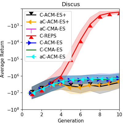
An interesting result, however, is that C-REPS is often much faster in the early phase. See, for example, Figure 3. In the first 10 generations, which amounts to 500 episodes, C-REPS outperforms all variants of C-CMA-ES by orders of magnitude. Unfortunately this is the phase of the optimization that is usually interesting for learning in the real world. We can also see that C-REPS converges already and does not learn anything for the next 840 generations. Variants of C-CMA-ES will continue making progress until the last episode. Because the surrogate model is only useful when we have a good estimate of the covariance matrix and a substantial amount of samples from the objective function, we can only use it in later stages of the optimization to improve the learning progress.
4.2. 2D Viapoint Problem
We will use a 2D viapoint problem. A dynamical movement primitive (Ijspeert et al. 2013) with , , , and 10 parameters per dimension will be used as trajectory representation. The reward is defined for each step as
and for the last step as the difference to each viapoint
Viapoints are defined as a tuple of time and positions , where .
We did not use C-REPS as a baseline because it is not robust against the choice of its hyperparameter (Fabisch et al. 2015). In the experiments, we use , , and a quadratic baseline. Learning curves are displayed in Figure 4. The performance is evaluated on a grid of 25 test contexts, where . Active C-CMA-ES does not make any difference. The convergence behavior of (a)C-ACM-ES is much better, however, the advantage only occurs after about 8,000 episodes, which is way too late for such a simple problem from the robotics perspective.
4.3. Ball Throwing
An example of a problem where it is much easier to define the reward function than the solution, is throwing a ball at a target. A reward is only given at the end of an episode, hence, we can directly define the return
where is the maximum velocity in a joint during execution of a robot’s throwing motion and is the point where the ball hits the ground. We define a problem which is very similar to the ball-throwing problem of Fabisch et al. 2015: a dynamical movement primitive represents a throwing movement of a 6 DOF robot with 10 weights per dimension. An initial movement hits the target . We try to generalize only over three arbitrarily selected contexts / target positions: , set , and .
Results are shown in Figure 5. The learning curve is very steep because the initial trajectory has to be adapted a lot to hit the new targets. We can set and to very low values because we only want to generalize over a set of three discrete contexts. In this case, using a surrogate model already gives a slight advantage so early in the learning process. The difference between active and standard covariance updates is not significant.
5. Conclusion and Outlook
We demonstrated that the extensions active C-CMA-ES and C-ACM-ES can be combined and yield impressive results on contextual function optimization problems in comparison to C-CMA-ES. We have shown, however, that these results are actually not directly transferable to the domain of robotics. We would like to learn successful upper-level policies in 100–1000 episodes at maximum. The presented extensions, however, start to be better than standard C-CMA-ES just after the range of interest. They exhibit much better convergence behavior though.
A drawback of many contextual optimization algorithms (for example, C-REPS and C-CMA-ES) is that they learn linear upper-level policies. The choice of defines the functions that can be represented. BO-CPS does not have this drawback because the policy is represented implicitly as an optimization problem over a global surrogate model similar to how policies are defined in value iteration reinforcement learning or Q-learning. This is expensive to compute though. More complex upper-level policies in C-CMA-ES would be an option to mitigate this restriction. We cannot say yet if more complex models are stable enough to be learned in practice.
Acknowledgements.
This work received funding from the European Union’s Horizon 2020 research and innovation program under grant agreement No 723853.References
- (1)
- Abdolmaleki et al. (2015) Abbas Abdolmaleki, Rudolf Lioutikov, Jan R Peters, Nuno Lau, Luis Pualo Reis, and Gerhard Neumann. 2015. Model-Based Relative Entropy Stochastic Search. In Advances in Neural Information Processing Systems 28. 3537–3545.
- Abdolmaleki et al. (2017a) A. Abdolmaleki, B. Price, N. Lau, L.P. Reis, and G. Neumann. 2017a. Contextual Covariance Matrix Adaptation Evolutionary Strategies. In IJCAI. 1378–1385.
- Abdolmaleki et al. (2017b) A. Abdolmaleki, D. Simões, N. Lau, L.P. Reis, and G. Neumann. 2017b. Learning a Humanoid Kick with Controlled Distance. In RoboCup. Springer, 45–57.
- Abdolmaleki et al. (2019) Abbas Abdolmaleki, David Simões, Nuno Lau, Luis Paulo Reis, and Gerhard Neumann. 2019. Contextual Direct Policy Search with Regularized Covariance Matrix Estimation. Journal of Intelligent and Robotic Systems (2019), 1–17. https://doi.org/10.1007/s10846-018-0968-4
- Brochu et al. (2010) Eric Brochu, Vlad M. Cora, and Nando de Freitas. 2010. A Tutorial on Bayesian Optimization of Expensive Cost Functions, with Application to Active User Modeling and Hierarchical Reinforcement Learning. eprint arXiv:1012.2599. arXiv.org.
- Deisenroth et al. (2013) M.P. Deisenroth, G. Neumann, and J. Peters. 2013. A Survey on Policy Search for Robotics. Foundations and Trends in Robotics 2, 1–2 (2013), 1–142.
- Fabisch and Metzen (2014) A. Fabisch and J.H. Metzen. 2014. Active Contextual Policy Search. Journal of Machine Learning Research 15 (2014), 3371–3399.
- Fabisch et al. (2015) A. Fabisch, J.H. Metzen, M.M. Krell, and F. Kirchner. 2015. Accounting for Task-Difficulty in Active Multi-Task Robot Control Learning. KI - Künstliche Intelligenz 29, 4 (2015), 369–377.
- Hansen et al. (2016) N. Hansen, A. Auger, O. Mersmann, T. Tusar, and D. Brockhoff. 2016. COCO: A Platform for Comparing Continuous Optimizers in a Black-Box Setting. CoRR abs/1603.08785 (2016).
- Hansen and Ostermeier (2001) N. Hansen and A. Ostermeier. 2001. Completely Derandomized Self-Adaptation in Evolution Strategies. Evolutionary Computation 9, 2 (2001), 159–195.
- Ijspeert et al. (2013) A.J. Ijspeert, J. Nakanishi, H. Hoffmann, P. Pastor, and S. Schaal. 2013. Dynamical movement primitives: learning attractor models for motor behaviors. Neural Computation 25, 2 (2013), 328–373.
- Jastrebski and Arnold (2006) G.A. Jastrebski and D.V. Arnold. 2006. Improving Evolution Strategies through Active Covariance Matrix Adaptation. In CEC. 2814–2821.
- Karkus et al. (2016) Péter Karkus, Andras Kupcsik, David Hsu, and Wee Sun Lee. 2016. Factored Contextual Policy Search with Bayesian Optimization. CoRR abs/1612.01746 (2016). arXiv:1612.01746 http://arxiv.org/abs/1612.01746
- Kober et al. (2013) J. Kober, J.A. Bagnell, and J. Peters. 2013. Reinforcement Learning in Robotics: A Survey. International Journal of Robotics Research (2013).
- Kober et al. (2012) Jens Kober, Andreas Wilhelm, Erhan Oztop, and Jan Peters. 2012. Reinforcement learning to adjust parametrized motor primitives to new situations. Autonomous Robots 33, 4 (2012), 361–379.
- Kupcsik et al. (2013) A.G. Kupcsik, M.P. Deisenroth, J. Peters, and G. Neumann. 2013. Data-Efficient Generalization of Robot Skills with Contextual Policy Search. In AAAI.
- Loshchilov et al. (2010) I. Loshchilov, M. Schoenauer, and M. Sebag. 2010. Comparison-Based Optimizers Need Comparison-Based Surrogates. In PPSN. Springer, 364–373.
- Metzen et al. (2015) J.H. Metzen, A. Fabisch, and J. Hansen. 2015. Bayesian Optimization for Contextual Policy Search. In MLPC-2015. IROS, Hamburg.
- Metzen (2015) Jan Hendrik Metzen. 2015. Active Contextual Entropy Search. In Proceedings of NIPS Workshop on Bayesian Optimization. Montreal, Quebec, Canada, 5. http://arxiv.org/abs/1511.04211
- Metzen (2016) Jan Hendrik Metzen. 2016. Minimum Regret Search for Single- and Multi-Task Optimization. In Proceedings of 33rd International Conference on Machine Learning (ICML). New York, NY, USA, 10. http://arxiv.org/abs/1602.01064
- Neumann (2011) G. Neumann. 2011. Variational Inference for Policy Search in changing situations. In Proceedings of the 28th International Conference on Machine Learning.
- Peters et al. (2010) J. Peters, K. Mülling, and Y. Altun. 2010. Relative Entropy Policy Search. In AAAI.
- Peters and Schaal (2007) Jan Peters and Stefan Schaal. 2007. Reinforcement learning by reward-weighted regression for operational space control. In Proceedings of the International Conference on Machine Learning. 745–750.
- Platt (1998) John Platt. 1998. Sequential Minimal Optimization: A Fast Algorithm for Training Support Vector Machines. Technical Report MSR-TR-98-14. Microsoft Research.
- Tangkaratt et al. (2017) Voot Tangkaratt, Herke van Hoof, Simone Parisi, Gerhard Neumann, Jan Peters, and Masashi Sugiyama. 2017. Policy Search with High-Dimensional Context Variables. In Proceedings of the 31st AAAI Conference on Artificial Intelligence. 2632–2638.