跳到论文正文
W Papers独立论文阅读器 arXiv:1810.11487 论文正文 计算阅读时间 · 0%
引用这篇论文根据当前论文元数据生成,正式投稿前建议核对。


License: arXiv.org perpetual non-exclusive license
arXiv:1810.11487v1 [cond-mat.mes-hall] 26 Oct 2018

A transformation optics approach to singular metasurfaces

Fan Yang Affiliation: The Blackett Laboratory
Department of Physics
Imperial College London
London SW7 2AZ, UK
   Paloma A. Huidobro Affiliation: The Blackett Laboratory
Department of Physics
Imperial College London
London SW7 2AZ, UK
   John B. Pendry Affiliation: The Blackett Laboratory
Department of Physics
Imperial College London
London SW7 2AZ, UK
Abstract

Surface plasmons dominate the optical response of metal surfaces, and their nature is controlled by surface geometry. Here we study metasurfaces containing singularities in the form of sharp edges and characterized by three quantum numbers despite the two-dimensional nature of the surface. We explore the nature of the plasmonic excitations, their ability to generate large concentrations of optical energy, and the transition from the discrete excitation spectrum of a non-singular surface to the continuous spectrum of a singular metasurface.

I Introduction

In a previous paper Pendry et al. 2017 we commented on the curious mathematical structure of the spectra of singular surfaces which are characterized by three quantum numbers despite the two-dimensional nature of the surface. Transformation optics Ward and Pendry 1996; Pendry et al. 2006 shows how the third dimension is hidden within the singularity Pendry et al. 2017. This paper will explore in detail the nature of the plasmonic excitations, their ability to generate large concentrations of optical energy, and the transition from the discrete excitation spectrum of a non-singular surface to the continuous spectrum of a singular metasurface. Sub-wavelength metal gratings couple external light into surface plasmons, efficiently localizing the electromagnetic energy and finding applications in optical bio-sensing and photovoltaics Wen et al. 2014; Munday and Atwater 2011; Dhawan et al. 2011; Bog et al. 2012; Kuo et al. 2012. These can be used to control external radiation using metasurfaces Holloway et al. 2012; Lin et al. 2014. Here we consider a singular metasurface. Singularities in plasmonic systems, such as sharp edges or touching points, concentrate the electromagnetic fields even to sub-nanometric volumes yielding huge energy densities Kelly et al. 2003; Prodan et al. 2003; Hao and Schatz 2004; Nordlander et al. 2004; Lu et al. 2005; Romero et al. 2006; Bukasov and Shumaker-Parry 2007; Romero et al. 2008; Wu et al. 2009; Aubry et al. 2010a; Luo et al. 2010; Benz et al. 2016; Galiffi et al. 2018.

Transformation optics takes advantage of the coordinate invariance of Maxwell’s equations to give a prescription of how the electromagnetic parameters ϵ\epsilon and μ\mu change under geometrical transformations. For the case of two-dimensional conformal transformations, ϵ\epsilon and μ\mu are left unchanged in the plane, which can be exploited for solving complex plasmonics problems by transforming them to a frame where geometry is simpler Pendry et al. 2012. This is particularly useful when considering systems with singularities Luo et al. 2010 as they give rise to divergences that cannot be treated exactly with numerical methods.

In this paper we use transformation optics to derive an analytical theory of the optical response of singular plasmonic metasurfaces. In previous works we have applied this framework to the study of metasurfaces with a smooth shape Kraft et al. 2015; Huidobro et al. 2017. Here we use the conformal transformation introduced in Ref. Pendry et al. 2017 for the design of singular metasurfaces, and present an analytical derivation to completely characterize its optical properties.

The text is structured as follows. First, in Section II we present the conformal transformation that generates a metasurface with grooves or wedges forming a sharp angle. The external fields incident on the metasurface are considered in Sec. III. Next, in Sec. IV we derive the analytical expressions for the electromagnetic fields and absorption cross section in the metasurface. We then introduce in Sec. V a flat surface model from which we obtain an effective surface conductivity that allows us to unambiguously determine the optical response of the metasurface through its reflectivity. Finally, the results for the singular metasurface at normal incidence are presented in Sec. VI, and for two cases which break the symmetry in Sec. VII: a symmetric metasurface under oblique incidence and an asymmetric metasurface.

II Creating a singular metasurface

We start by describing the transformations that result in the singular metasurfaces shown in Fig. 1. Let us first consider an array of metal slabs with periodicity along the vertical direction and translational invariance along the horizontal direction, placed in the slab frame (z1=x1+i​y1z_{1}=x_{1}+iy_{1}). The period of the array is dd, the thickness of the slabs is d3d_{3} and we take d1+d2d_{1}+d_{2} to be the thickness of the dielectric region. An exponential transformation maps the slab array into either a wedge when d1+d2>d3d_{1}+d_{2}>d_{3} [panel (a)], or a groove when d1+d2<d3d_{1}+d_{2}<d_{3} [see panel (b)], in frame z2z_{2}. Then an inverse transformation is carried out to get the two-touching-circular segments shown in the z3z_{3} frame. As a last step, a logarithmic transformation is used to generate a surface with a periodic set of sharp wedges/grooves (see z4z_{4} frame): these are the singular metasurfaces under consideration here.

Refer to caption
Figure 1: A series of transformations to generate a singular metasurface with (a) concave shape (d1+d2>d3d_{1}+d_{2}>d_{3}) and (b) convex shape (d1+d2<d3d_{1}+d_{2}<d_{3}). The different coordinate frames are labelled as ziz_{i}, with zi=xi+i​yiz_{i}=x_{i}+iy_{i}. In the slab frame, z1z_{1}, the period of the slab array is dd, d1+d2d_{1}+d_{2} is the thickness of the air region and d3d_{3} is the thickness of each metal slab. This is successively transformed to a single wedge/groove (frame z2z_{2}), two-touching-circular segments (frame z3z_{3}) and finally a singular metasurface (frame z4z_{4}). Note that x-axis and y-axis do not have the same scale.

On the basis of this series of transformations, a one-step transformation from the slab frame to the metasurface frame can be written as

z4=T2​π​ln​(1a⁡(e2​π​z1/d−1)+12​a)\begin{split}z_{4}=\frac{T}{2\pi}\mathrm{ln}\bigg(\frac{1}{a(e^{2\pi z_{1}/d}-1)}+\frac{1}{2a}\bigg)\end{split} (1)

Here, TT defines the size of the metasurface by fixing its period, and aa is chosen as 0.5 so that the singular point in the metasurface frame is located on the y-axis. As mentioned previously, d=d1+d2+d3d=d_{1}+d_{2}+d_{3} is the periodicity in the slab frame, and the choice of {d1,d2,d3}\{d_{1},d_{2},d_{3}\} determines the shape of the metasurface. For d1+d2=d3d_{1}+d_{2}=d_{3} the transformation generates a flat surface, while d1+d2>(<)​d3d_{1}+d_{2}>(<)d_{3} results in concave (convex) singular metasurfaces formed by periodic sharp wedges (grooves). In addition, setting d1=d2d_{1}=d_{2} generates a metasurface that is symmetric with respect to the horizontal axis.

In the following we detail our analytical derivations to calculate the optical response of these singular metasurfaces. Throughout the paper we take the metal to be gold with permittivity approximated by the Drude model, ε=1−ωp2ω⁡(ω+i​Γ)\varepsilon=1-\frac{\omega_{p}^{2}}{\omega(\omega+i\Gamma)}, with plasma frequency ωp=8.95\omega_{p}=8.95 eV/ℏ\hbar and damping Γ=65.8\Gamma=65.8 meV/ℏ\hbar Novotny and Hecht 2012.

III Transforming the source

The problem we set out to solve is that of a p-polarized plane wave (magnetic field out of the plane, HzH_{z}) incident on the singular metasurface, as any more complex wave front can be expressed as a superposition of plane waves. Since the transformation not only transforms the geometry but also the form of the source, we have to derive the representation of the source in the slab frame. For this purpose, we generate an incident wave using a periodic array of magnetic current line sources (“monopoles”) in the right hand-side of the metasurface frame, as depicted in Fig. 2(b). Taking the sources to be at infinity such that their near fields can be safely neglected Pendry and Gard 1975; Tretyakov 2003, their radiated field is a plane wave incident on the surface. We assume that the period of the metasurface is much less than the free space wavelength. When the incident wave impinges on the singular surface, there will be reflected and transmitted waves. These three sorts of waves all participate in the excitation of surface plasmons at the singular surface. In addition to the source currents, there needs to be a sink at infinity to receive the reflected waves, and another sink at minus infinity to receive the transmitted waves. Then, the source in the slab frame can be obtained by recognising that: (i) a magnetic current line is conserved under the transformation and, (ii) sources at +∞+\infty in the metasurface frame are mapped to the point z1=i​n​dz_{1}=ind while sources at −∞-\infty in the metasurface frame are mapped to z1=i⁡(n+12)​dz_{1}=i(n+\frac{1}{2})d (here nn is an integer). Hence, the monopole sources generating the incident wave and the monopoles receiving the reflected waves are located in the air region in the slab frame, while the monopoles receiving the transmitted wave are placed in the metal region [see Fig. 2(a)].

We start by writing the magnetic field of the incident, reflected and transmitted waves in the metasurface frame as,

{Hzi​n​c=H0​e−i​k0​x​x4+i​k0​y​y4Hzr​e​f=r​H0​ei​k0​x​x4+i​k0​y​y4Hzt​r​a=tH0e−ik0​x′x4+ik0​yy4\left\{{\begin{array}[]{l}H_{z}^{inc}=H_{0}e^{-ik_{0x}x_{4}+ik_{0y}y_{4}}\\ H_{z}^{ref}=rH_{0}e^{ik_{0x}x_{4}+ik_{0y}y_{4}}\\ H_{z}^{tra}=tH_{0}e^{-ik_{0x}^{{}^{\prime}}x_{4}+ik_{0y}y_{4}}\end{array}}\right. (2)

where H0H_{0} is the wave amplitude, rr and tt are reflection and transmission coefficients, k0​x=k02−k0​y2k_{0x}=\sqrt{k_{0}^{2}-k_{0y}^{2}} and k0​x′=ε​k02−k0​y2k_{0x}^{{}^{\prime}}=\sqrt{\varepsilon k_{0}^{2}-k_{0y}^{2}}.

Refer to caption
Figure 2: Sketch showing the source field in both frames. In the metasurface frame (b) the source is a plane wave incident on the surface, which we take to be generated by an array of magnetic line currents located at infinity. The source is mapped into an array of magnetic line currents in the slab frame (a).

In order to write the source field in the slab frame, we transform Eq. 2 using the mapping Eq. (1) to obtain,

{Hzi​n​c=H0​(1+i​k0​x​T2​π​ln​(πd))+∫−∞∞aa​e−|kx|​|y1||kx|​ei​kx​x1​d​kx+∫−∞∞as​e−|kx|​|y1|s​g​n​(y1)​kx​ei​kx​x1​d​kxHzr​e​f=r​H0​(1−i​k0​x​T2​π​ln​(πd))−∫−∞∞r​aa​e−|kx|​|y1||kx|​ei​kx​x1​d​kx+∫−∞∞r​as​e−|kx|​|y1|s​g​n​(y1)​kx​ei​kx​x1​d​kxHzt​r​a=t​H0​(1−i​k0​x′T2​π​ln​(πd))−∫−∞∞t​k0​x′k0​x​aa​e−|kx|​|y1||kx|​ei​kx​x1​d​kx−∫−∞∞t​as​e−|kx|​|y1+d2|s​g​n​(y1+d2)​kx​ei​kx​x1​d​kx\left\{{\begin{array}[]{l}H_{z}^{inc}=H_{0}\bigg(1+i\frac{k_{0x}T}{2\pi}\mathrm{ln}\big(\frac{\pi}{d}\big)\bigg)+\int\limits_{-\infty}^{\infty}a_{a}\frac{e^{-|k_{x}||y_{1}|}}{|k_{x}|}e^{ik_{x}x_{1}}dk_{x}+\int\limits_{-\infty}^{\infty}a_{s}\frac{e^{-|k_{x}||y_{1}|}}{sgn(y_{1})k_{x}}e^{ik_{x}x_{1}}dk_{x}\\ H_{z}^{ref}=rH_{0}\bigg(1-i\frac{k_{0x}T}{2\pi}\mathrm{ln}\big(\frac{\pi}{d}\big)\bigg)-\int\limits_{-\infty}^{\infty}ra_{a}\frac{e^{-|k_{x}||y_{1}|}}{|k_{x}|}e^{ik_{x}x_{1}}dk_{x}+\int\limits_{-\infty}^{\infty}ra_{s}\frac{e^{-|k_{x}||y_{1}|}}{sgn(y_{1})k_{x}}e^{ik_{x}x_{1}}dk_{x}\\ H_{z}^{tra}=tH_{0}\bigg(1-i\frac{k_{0x}^{{}^{\prime}}T}{2\pi}\mathrm{ln}\big(\frac{\pi}{d}\big)\bigg)-\int\limits_{-\infty}^{\infty}t\frac{k_{0x}^{{}^{\prime}}}{k_{0x}}a_{a}\frac{e^{-|k_{x}||y_{1}|}}{|k_{x}|}e^{ik_{x}x_{1}}dk_{x}-\int\limits_{-\infty}^{\infty}ta_{s}\frac{e^{-|k_{x}||y_{1}+\frac{d}{2}|}}{sgn(y_{1}+\frac{d}{2})k_{x}}e^{ik_{x}x_{1}}dk_{x}\end{array}}\right. (3)

The detailed derivation for these source representations is included in Appendix A. In writing the above equations we have assumed that the period of the metasurface is subwavelength (T≪|x4|≪λT\ll|x_{4}|\ll\lambda). Also, we have written the fields as a Fourier series and we have identified a symmetric and an antisymmetric component to the source with amplitudes aa=−i​k0​x​T4​π​H0a_{a}=-i\frac{k_{0x}T}{4\pi}H_{0} (anti-symmetric source) and as=k0​y​T4​π​H0a_{s}=\frac{k_{0y}T}{4\pi}H_{0} (symmetric source). Note that we define the symmetry of the modes by considering the ExE_{x} component in the slab frame: the anti-symmetric (symmetric) mode has odd (even) symmetry of Ex​(y)E_{x}(y). From the above, we can write the source field in k-space for the antisymmetric mode as,

Hza​(kx)={(1−r)​aa​e−|kx|​|y||kx|,−d2<y<d1−t​k0​x′k0​x​aa​e−|kx|​|y+d2||kx|,−d2+d3<y<−d2H_{z}^{a}(k_{x})=\left\{{\begin{array}[]{lr}(1-r)a_{a}\frac{e^{-|k_{x}||y|}}{|k_{x}|},&{-{d_{2}}<y<{d_{1}}}\\ -t\frac{k_{0x}^{{}^{\prime}}}{k_{0x}}a_{a}\frac{e^{-|k_{x}||y+\frac{d}{2}|}}{|k_{x}|},&{-{d_{2}+d_{3}}<y<{-d_{2}}}\end{array}}\right. (4)

and for the symmetric mode as,

Hzs​(kx)={(1+r)​as​sgn​(kx)​e−|kx|​|y|sgn​(y)​|kx|,−d2<y<d1−t​as​sgn​(kx)​e−|kx|​|y+d2|sgn​(y+d2)​|kx|,−d2+d3<y<−d2H_{z}^{s}(k_{x})=\left\{{\begin{array}[]{lr}(1+r)a_{s}\text{sgn}(k_{x})\frac{e^{-|k_{x}||y|}}{\text{sgn}(y)|k_{x}|},&{-{d_{2}}<y<{d_{1}}}\\ -ta_{s}\text{sgn}(k_{x})\frac{e^{-|k_{x}||y+\frac{d}{2}|}}{\text{sgn}(y+\frac{d}{2})|k_{x}|},&{-{d_{2}+d_{3}}<y<{-d_{2}}}\end{array}}\right. (5)

in which the constant field components are ignored since they do not contribute to the excitation of surface plasmon polaritons. Finally, note that the source representation includes terms ∼e−|kx|​|y||kx|\sim\frac{e^{-|k_{x}||y|}}{|k_{x}|}, which is just the Fourier transformation of a Hankel function in the quasi-static limit Chew 1995. Indeed, a Hankel function is the source representation of a line current, which further confirms our source representation.

IV Electromagnetic fields and absorption cross section

IV.1 Surface plasmons dispersion relation

Once we have the source fields, we can calculate the excited field components. When a SPP mode (Hz∼ei​kx​xH_{z}\sim e^{ik_{x}x}) on the boundary between metal and air is excited, the total field distribution in the slab frame can be written as

Hz​(kx)={(1−r)​aa​e−|kx|​|y||kx|+(1+r)​as​e−|kx|​|y|sgn​(y)​kx+b+​e−|kx|​y+b−​e|kx|​y,−d2<y<d1−t​k0​x′k0​x​aa​e−|kx|​|y+d2||kx|−t​as​e−|kx|​|y+d2|sgn​(y+d2)​kx+c+​e−|kx|​y+c−​e|kx|​y,−(d2+d3)<y<−d2H_{z}(k_{x})=\left\{{\begin{array}[]{lr}(1-r)a_{a}\frac{e^{-|k_{x}||y|}}{|k_{x}|}+(1+r)a_{s}\frac{e^{-|k_{x}||y|}}{\text{sgn}(y)k_{x}}+{b_{+}}e^{-|k_{x}|y}+{b_{-}}e^{|k_{x}|y},&{-d_{2}<y<d_{1}}\\ -t\frac{k_{0x}^{{}^{\prime}}}{k_{0x}}a_{a}\frac{e^{-|k_{x}||y+\frac{d}{2}|}}{|k_{x}|}-ta_{s}\frac{e^{-|k_{x}||y+\frac{d}{2}|}}{\text{sgn}(y+\frac{d}{2})k_{x}}+{c_{+}}e^{-|k_{x}|y}+{c_{-}}e^{|k_{x}|y},&{-({d_{2}}+{d_{3}})<y<-{d_{2}}}\end{array}}\right. (6)

Here, b+b_{+}, b−b_{-}, c+c_{+} and c−c_{-} are the excited mode amplitudes, which have to be determined from the boundary conditions. This requires matching the tangent components of the fields, HzH_{z} and ExE_{x}, at y=d1y=d_{1}, y=−d2y=-d_{2} and y=−(d2+d3)y=-(d_{2}+d_{3}) Luo et al. 2010 and details are given in Appendix B.

Refer to caption
Figure 3: Dispersion relations of surface plasmons in singular metasurfaces. (a), (c) SPP dispersion relation in a wedge singular metasurface at oblique (a) and normal incidence (c). The parameters are d3=0.1​dd_{3}=0.1d, d1=d2=(d−d3)/2d_{1}=d_{2}=(d-d_{3})/2.(b), (d) SPP dispersion relation in a groove singular metasurface at oblique (b) and normal incidence (d). The parameters are d3=0.9​dd_{3}=0.9d, d1=d2=(d−d3)/2d_{1}=d_{2}=(d-d_{3})/2.

Once the excited field mode amplitudes have been determined (see Eqs. B2-B5), the dispersion relation of surface plasmons can be obtained by looking at the poles of these coefficients. Neglecting the pole kx=0k_{x}=0 as it is a branch point which corresponds to a localized virtual excitation rather than SPPs Aubry et al. 2010b; Aubry et al. 2010c, we concentrate on the plasmon pole. From the amplitude of the anti-symmetric mode (Eqs. B2 and B3), we obtain

(ε−1)​(e|kx|​(d1+d2)−e|kx|​d3)+(ε+1)​(e|kx|​d−1)=0\begin{split}(\varepsilon-1)(e^{|k_{x}|(d_{1}+d_{2})}-e^{|k_{x}|d_{3}})+(\varepsilon+1)(e^{|k_{x}|d}-1)=0\end{split} (7)

While for the symmetric mode (Eqs. B4 and B5) we have,

(ε−1)​(e|kx|​(d1+d2)−e|kx|​d3)−(ε+1)​(e|kx|​d−1)=0\begin{split}(\varepsilon-1)(e^{|k_{x}|(d_{1}+d_{2})}-e^{|k_{x}|d_{3}})-(\varepsilon+1)(e^{|k_{x}|d}-1)=0\end{split} (8)

Figure 3 shows the calculated dispersion relations for the singular wedge (a, c) and groove (b, d) metasurfaces. For the general case, at an oblique incidence, both the symmetric and antisymmetric bands can be excited, as shown in panels (a) and (b). On the other hand, at normal incidence only the antisymmetric band is excited [panels (c) and (d)]. It should be noted that the bands have lower and upper cut-off frequencies different from 0 and ωp\omega_{p}. For the wedge (groove) metasurface, the symmetric (antisymmetric) band spans a frequency range ωc​1≤ω<ωs​p\omega_{c1}\leq\omega<\omega_{sp} while the antisymmetric (symmetric band) spans ωs​p<ω≤ωc​2\omega_{sp}<\omega\leq\omega_{c2}. Here, ωs​p\omega_{sp} is the surface plasmon frequency, and ωc⁡(1,2)\omega_{c(1,2)} are the lower and upper cut-off frequencies, which were shown to be ωc​1=ωp​θ2​π\omega_{c1}=\omega_{p}\sqrt{\frac{\theta}{2\pi}} and ωc​2=ωp​2​π−θ2​π\omega_{c2}=\omega_{p}\sqrt{\frac{2\pi-\theta}{2\pi}}, where θ=2​π​d3d\theta=2\pi\frac{d_{3}}{d} for the wedge case (d1+d2>d3d_{1}+d_{2}>d_{3}), θ=2​π​d1+d2d\theta=2\pi\frac{d_{1}+d_{2}}{d} for the groove case (d1+d2<d3d_{1}+d_{2}<d_{3}) Luo et al. 2010. The appearance of these cut-offs is a result of plasmon hybridization in the infinite periodic array of the slab frame Luo et al. 2010. Note that when analyzing the dispersion relation, we have assumed a lossless metal, while we use a finite damping for the rest of the paper.

In the following we focus on the groove singular metasurface, for which the antisymmetric band excited at normal incidence exists below ωs​p\omega_{sp}, where the Drude model gives a more accurate description of the metal.

IV.2 Electric and magnetic fields in real space

Next, we calculate the electromagnetic fields in real space. We write the SPP mode field distribution by taking the Fourier transform of the excited terms in the magnetic field given by Eq. (6),

Hz​(x,y)=∫−∞∞Hz​(kx,y)​ei​kx​x​d​kx=2​π​i​Res​[Hz​(kx,y)​ei​kx​x]|kx=kp​xH_{z}(x,y)=\int\limits_{-\infty}^{\infty}H_{z}(k_{x},y)e^{i{k_{x}}x}d{k_{x}}=2\pi i\text{Res}\left[H_{z}(k_{x},y)e^{i{k_{x}}x}\right]|_{k_{x}=k_{px}} (9)

where the residue theorem is applied at the plasmon pole, kx=kp​xk_{x}=k_{px}. Also, from Eq. (6) we have Hz​(kx,y)=b+​e−|kx|​y+b−​e|kx|​yH_{z}(k_{x},y)={b_{+}}e^{-|k_{x}|y}+{b_{-}}e^{|k_{x}|y} in the dielectric region and Hz​(kx,y)=c+​e−|kx|​y+c−​e|kx|​yH_{z}(k_{x},y)={c_{+}}e^{-|k_{x}|y}+{c_{-}}e^{|k_{x}|y} in the metal region. This yields the following field distribution in the slab frame:

Hz​(x,y)={i​2​π​a​(Γ+​e−kp​x2​y+Γ−​ekp​x2​y)​ei​kp​x​|x|,−d2<y<d1i​2​π​a​(Λ+​e−kp​x2​y+Λ−​ekp​x2​y)​ei​kp​x​|x|,−d2+d3<y<−d2H_{z}(x,y)=\left\{{\begin{array}[]{lr}i2\pi a({\Gamma_{+}}{e^{-{\sqrt{k_{px}^{2}}}y}}+{\Gamma_{-}}{e^{{\sqrt{k_{px}^{2}}}y}})e^{i{k_{px}}|x|},&{-{d_{2}}<y<{d_{1}}}\\ i2\pi a({\Lambda_{+}}{e^{-{\sqrt{k_{px}^{2}}}y}}+{\Lambda_{-}}{e^{{\sqrt{k_{px}^{2}}}y}})e^{i{k_{px}}|x|},&{-{d_{2}+d_{3}}<y<-{d_{2}}}\end{array}}\right. (10)

where aa stands for a(a,s)a_{(a,s)} for the antisymmetric/symmetric mode and |kx||k_{x}| has been written as kx2\sqrt{k_{x}^{2}} in the complex integration. All the field coefficients (Γ+\Gamma_{+}, Γ−\Gamma_{-}, Λ+\Lambda_{+} and Λ−\Lambda_{-}) are given in Appendix B (Eqs. B6-B9). The electric field can be derived from Maxwell’s equations using Ex=iω​ε​∂Hz∂yE_{x}=\frac{i}{\omega\varepsilon}\frac{\partial{H_{z}}}{\partial{y}},

Ex​(x,y)={2​π​a​kp​x2ω​ε0​(Γ+​e−kp​x2​y−Γ−​ekp​x2​y)​ei​kp​x​|x|,−d2<y<d12​π​a​kp​x2ω​ε0​ε​(Λ+​e−kp​x2​y−Λ−​ekp​x2​y)​ei​kp​x​|x|,−d2+d3<y<−d2E_{x}(x,y)=\left\{{\begin{array}[]{lr}\frac{2\pi a\sqrt{k_{px}^{2}}}{\omega\varepsilon_{0}}({\Gamma_{+}}{e^{-{\sqrt{k_{px}^{2}}}y}}-{\Gamma_{-}}{e^{{\sqrt{k_{px}^{2}}}y}})e^{i{k_{px}}|x|},&{-{d_{2}}<y<{d_{1}}}\\ \frac{2\pi a\sqrt{k_{px}^{2}}}{\omega\varepsilon_{0}\varepsilon}({\Lambda_{+}}{e^{-{\sqrt{k_{px}^{2}}}y}}-{\Lambda_{-}}{e^{{\sqrt{k_{px}^{2}}}y}})e^{i{k_{px}}|x|},&{-{d_{2}+d_{3}}<y<-{d_{2}}}\end{array}}\right. (11)

and Ey=−iω​ε​∂Hz∂xE_{y}=-\frac{i}{\omega\varepsilon}\frac{\partial{H_{z}}}{\partial{x}},

Ey​(x,y)={i​sgn​(x)​2​π​a​kp​xω​ε0​(Γ+​e−kp​x2​y+Γ−​ekp​x2​y)​ei​kp​x​|x|,−d2<y<d1i​sgn​(x)​2​π​a​kp​xω​ε0​ε​(Λ+​e−kp​x2​y+Λ−​ekp​x2​y)​ei​kp​x​|x|,−d2+d3<y<−d2E_{y}(x,y)=\left\{{\begin{array}[]{lr}i\text{sgn}(x)\frac{2\pi ak_{px}}{\omega\varepsilon_{0}}({\Gamma_{+}}{e^{-{\sqrt{k_{px}^{2}}}y}}+{\Gamma_{-}}{e^{{\sqrt{k_{px}^{2}}}y}})e^{i{k_{px}}|x|},&{-{d_{2}}<y<{d_{1}}}\\ i\text{sgn}(x)\frac{2\pi ak_{px}}{\omega\varepsilon_{0}\varepsilon}({\Lambda_{+}}{e^{-{\sqrt{k_{px}^{2}}}y}}+{\Lambda_{-}}{e^{{\sqrt{k_{px}^{2}}}y}})e^{i{k_{px}}|x|},&{-{d_{2}+d_{3}}<y<-{d_{2}}}\end{array}}\right. (12)
Refer to caption
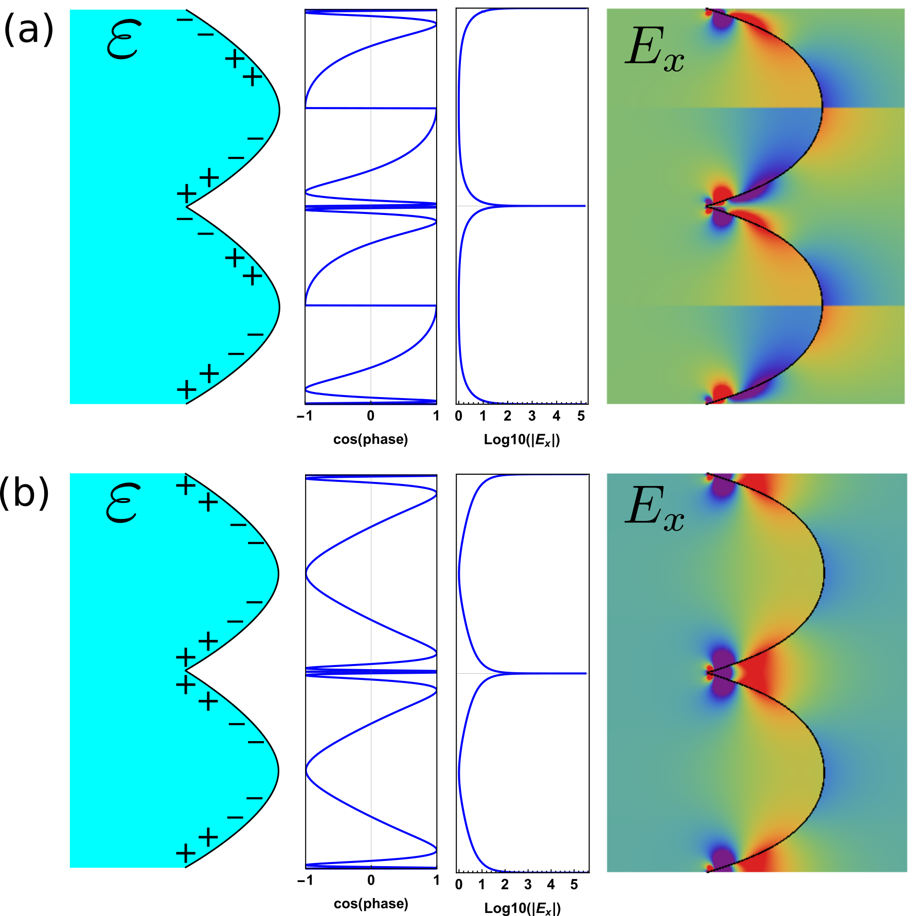
Figure 4: Mode plot of ExE_{x} in the metasurface frame for (a) anti-symmetric mode at ω=0.6​ωp\omega=0.6\omega_{p} and (b) symmetric mode at ω=0.8​ωp\omega=0.8\omega_{p}. From left column to right column are: charge distribution (sketch), phase and amplitude along the singular surface, and field distribution in the unit cell. The parameters are: d3=0.9​dd_{3}=0.9d, d1=d2=(d−d3)/2d_{1}=d_{2}=(d-d_{3})/2. In the color map, red stands for positive values of the field magnitude and blue for negative ones.

Once we have the fields in the slab frame, the fields in the metasurface frame can be calculated by mapping them following the rules of transformation opticsWard and Pendry 1996; Pendry et al. 2006. The obtained mode profile is plotted in Fig. 4 for the antisymmetric (a) and symmetric (b) modes at two frequencies of choice below and above the surface plasmon frequency. We show a sketch of the charge distribution for each mode (antibonding and bonding, respectively), together with the calculated phase and amplitude of the ExE_{x} component along the singular surface, and a field plot for Ex​(x,y)E_{x}(x,y) in the metasurface frame. It is clear the phase oscillates very rapidly, and the in-plane electric field diverges at the singularity. This can be understood from the compression of an infinite dimension hidden at the singular point Pendry et al. 2017, making the derivative of HzH_{z} with respect to xx and yy to be infinite at the singularity. On the other hand, due to its invariance, the magnetic field keeps a finite value in all the frames shown in Fig. 1, and in particular in the singular metasurface frame.

The presence of loss will attenuate the field in any real system. In this case, the amplitude of the excited SPP wave in the slab frame will be attenuated as it travels along the slab and away from the sources. As was shown previously, there is a critical angle of the groove/wedge where the enhancement by compression and attenuation by loss are balanced Luo et al. 2010. The electric field converges for θ≤θc\theta\leq\theta_{c}, while it diverges otherwise, where θc=Im⁡[ln⁡(ε−1ε+1)]\theta_{c}=\mathrm{Im}[\mathrm{ln}\left(\frac{\varepsilon-1}{\varepsilon+1}\right)] for the lower band, and θc=−Im⁡[ln⁡(1−εε+1)]\theta_{c}=-\mathrm{Im}[\mathrm{ln}\left(\frac{1-\varepsilon}{\varepsilon+1}\right)] for the upper band. The geometrical parameters chosen in Fig. 4 (d3=0.9​dd_{3}=0.9d, d1=d2=(d−d3)/2d_{1}=d_{2}=(d-d_{3})/2) yield an angle at the singularity of θ=2​π​M​i​n​(d1+d2,d3)d=0.2​π\theta=2\pi\frac{Min(d_{1}+d_{2},d_{3})}{d}=0.2\pi. At the frequencies of choice, ω=0.6​ωp\omega=0.6\omega_{p} for the antisymmetric mode and ω=0.8​ωp\omega=0.8\omega_{p} for the symmetric one, the critical angles are θc=0.03\theta_{c}=0.03 and θc=0.04\theta_{c}=0.04, respectively. Therefore, the electric field at singular point of both anti-symmetric and symmetric modes diverges despite the presence material losses, as shown in the right column of Fig. 4.

IV.3 Energy dissipation by SPPs

Once the field distribution is obtained, we calculate the energy dissipated by the excited SPP mode in the slab frame. Dissipation is due to loss in the metal, so we calculate the absorbed power as the following integral on the slab volume,

Pa​b​s(a,s)=∫s​l​a​b12​ω​ε0​Im​[ε]​|E|2​𝑑x​𝑑y=4​π2​|a|2​|kp​x|2​Im​[ε]ω​ε0​|ε|2​(|Λ(a,s)+|2−2​R​e​[kp​x2]​(e2​R​e​[kp​x2]​d2−e2​R​e​[kp​x2]​(d2+d3CLOSE)CLOSEOPEN+|Λ(a,s)−|22​R​e​[kp​x2]​(e−2​R​e​[kp​x2]​d2−e−2​R​e​[kp​x2]​(d2+d3)))​1Im⁡[kp​x]\begin{split}P^{(a,s)}_{abs}&=\int\limits_{slab}\frac{1}{2}\omega\varepsilon_{0}\mathrm{Im}[\varepsilon]|E|^{2}dxdy\\ &=\frac{4\pi^{2}|a|^{2}|k_{px}|^{2}\mathrm{Im}[\varepsilon]}{\omega\varepsilon_{0}|\varepsilon|^{2}}(\frac{|\Lambda_{(a,s)+}|^{2}}{-2\mathrm{Re}[\sqrt{k_{px}^{2}}]}(e^{2\mathrm{Re}[\sqrt{k_{px}^{2}}]d_{2}}-e^{2\mathrm{Re}[\sqrt{k_{px}^{2}}](d_{2}+d_{3}})\\ &+\frac{|\Lambda_{(a,s)-}|^{2}}{2\mathrm{Re}[\sqrt{k_{px}^{2}}]}(e^{-2\mathrm{Re}[\sqrt{k_{px}^{2}}]d_{2}}-e^{-2\mathrm{Re}[\sqrt{k_{px}^{2}}](d_{2}+d_{3})})\big)\frac{1}{\mathrm{Im}[k_{px}]}\end{split} (13)

where the coefficients Λ(a,s)±\Lambda_{(a,s)\pm} stand for the antisymmetric and symmetric mode coefficients given in Eqs. (B7) and (B9). Using Λa±\Lambda_{a\pm} (Λs±\Lambda_{s\pm}) yields the power absorbed by the antisymmetric (symmetric) mode. Finally, the absorption cross section of the structure can be obtained by normalizing to the input energy on the system in one period,

σa​b​s(a,s)=Pa​b​s(a,b)12μ0ε0H02Tcosθi​n,\sigma^{(a,s)}_{abs}=\frac{P^{(a,b)}_{abs}}{\frac{1}{2}\sqrt{\frac{\mu_{0}}{\varepsilon_{0}}}H_{0}^{2}T\cos{\theta_{in}}}, (14)

where θi​n\theta_{in} is incident angle of the plane wave and H0H_{0} is the wave amplitude. Thus, we have for the anti-symmetric mode,

σa​b​sa=k0Tcosθi​n2​|kp​x|2​Im​[ε]|ε|2​(|Λa+|2−2​R​e​[kp​x2]​(e2​R​e​[kp​x2]​d2−e2​R​e​[kp​x2]​(d2+d3CLOSE)CLOSEOPEN+|Λa+|22​R​e​[kp​x2]​(e−2​R​e​[kp​x2]​d2−e−2​R​e​[kp​x2]​(d2+d3)))​1Im⁡[kp​x]\begin{split}\sigma_{abs}^{a}&=\frac{k_{0}T\cos{\theta_{in}}}{2}\frac{|k_{px}|^{2}\mathrm{Im}[\varepsilon]}{|\varepsilon|^{2}}(\frac{|\Lambda_{a+}|^{2}}{-2\mathrm{Re}[\sqrt{k_{px}^{2}}]}(e^{2\mathrm{Re}[\sqrt{k_{px}^{2}}]d_{2}}-e^{2\mathrm{Re}[\sqrt{k_{px}^{2}}](d_{2}+d_{3}})\\ &+\frac{|\Lambda_{a+}|^{2}}{2\mathrm{Re}[\sqrt{k_{px}^{2}}]}(e^{-2\mathrm{Re}[\sqrt{k_{px}^{2}}]d_{2}}-e^{-2\mathrm{Re}[\sqrt{k_{px}^{2}}](d_{2}+d_{3})})\big)\frac{1}{\mathrm{Im}[k_{px}]}\end{split} (15)

and for the symmetric one,

σa​b​ss=k0​T​sin2⁡θi​n2cosθi​n​|kp​x|2​Im​[ε]|ε|2​(|Λs+|2−2​R​e​[kp​x2]​(e2​R​e​[kp​x2]​d2−e2​R​e​[kp​x2]​(d2+d3CLOSE)CLOSEOPEN+|Λs+|22​R​e​[kp​x2]​(e−2​R​e​[kp​x2]​d2−e−2​R​e​[kp​x2]​(d2+d3)))​1Im⁡[kp​x]\begin{split}\sigma_{abs}^{s}&=\frac{k_{0}T\sin^{2}{\theta_{in}}}{2\cos{\theta_{in}}}\frac{|k_{px}|^{2}\mathrm{Im}[\varepsilon]}{|\varepsilon|^{2}}(\frac{|\Lambda_{s+}|^{2}}{-2\mathrm{Re}[\sqrt{k_{px}^{2}}]}(e^{2\mathrm{Re}[\sqrt{k_{px}^{2}}]d_{2}}-e^{2\mathrm{Re}[\sqrt{k_{px}^{2}}](d_{2}+d_{3}})\\ &+\frac{|\Lambda_{s+}|^{2}}{2\mathrm{Re}[\sqrt{k_{px}^{2}}]}(e^{-2\mathrm{Re}[\sqrt{k_{px}^{2}}]d_{2}}-e^{-2\mathrm{Re}[\sqrt{k_{px}^{2}}](d_{2}+d_{3})})\big)\frac{1}{\mathrm{Im}[k_{px}]}\end{split} (16)

IV.4 Metasurface with blunt singularities: From a continuous to a discrete spectrum

Any fabricated metasurface will not show a perfect singularity but a blunt one, so we now move on to treat blunt singularities Luo et al. 2012. A metasurface with rounded singularities maps into a truncated slab array (or truncated cavity array for the groove geometry), as shown in Fig. 5. This has an important consequence: when the slabs/cavities are not infinite, the excited SPP modes travelling along the slab will be reflected at its terminals, as depicted in Fig. 5(a), resulting in a quantization of the SPP modes supported by the slab structure. Hence, the continuous spectrum of a singular metasurface turns into a discrete spectrum when the singularities are blunt.

Refer to caption
Figure 5: Metasurface with blunt singularities. A periodic array of truncated slabs in the slab frame (a) maps to a metasurface with blunt singularities in the metasurface frame (b).

In order to calculate the field distribution and energy dissipation in the truncated slab/cavity arrays we first need to calculate the reflection coefficient of SPPs at the slab/cavity terminal. For conciseness, in the following we will refer only to the cavity array shown in Fig. 5 (a) and we point out here that the same derivation can be applied to the truncated slab array. The radius of the rounded singularity in the metasurface frame determines the length of the cavities in the slab frame, LL, as well as the exact shape of the terminal. In order to calculate the reflection coefficient of the SPP modes at the end of the cavity we assume that the terminal is a flat vertical air/metal interface. Then we consider the field of the SPP modes (Hzs​pH_{z}^{sp}) in the cavity, −L/2<x1<L/2-L/2<x_{1}<L/2, and the field (Hzo​u​tH_{z}^{out}) in the region outside the cavity, x1<−L/2x_{1}<-L/2 and x1>L/2x_{1}>L/2, and impose the continuity condition of the tangential fields and the power flow at x1=L/2x_{1}=L/2 Chandran et al. 2012; Gordon 2006. This yields the equations,

(1+rs​p)​Hzs​p\displaystyle(1+r_{sp})H_{z}^{sp} =\displaystyle= Hzo​u​t\displaystyle H_{z}^{out} (17)
(1−rs​p)​Eys​p\displaystyle(1-r_{sp})E_{y}^{sp} =\displaystyle= Eyo​u​t\displaystyle E_{y}^{out} (18)
∫−(d2+d3)d1(1−rs​p∗)(1+rs​p)Eysp∗Hzs​pdy\displaystyle\int\limits_{-(d_{2}+d_{3})}^{d_{1}}(1-r_{sp}^{*})(1+r_{sp})E_{y}^{sp*}H_{z}^{sp}dy =\displaystyle= ∫−(d2+d3)d1Eyout∗Hzo​u​tdy\displaystyle\int\limits_{-(d_{2}+d_{3})}^{d_{1}}E_{y}^{out*}H_{z}^{out}dy (19)

where, Hzs​pH_{z}^{sp} and Eys​pE_{y}^{sp} are given in Sec. IV.2.

In the region outside the periodic cavity array we expand the magnetic field as a series of Bloch waves,

Hzo​u​t=∑gh⁡(g)​ei​g​y\begin{split}H_{z}^{out}=\sum_{g}h(g)e^{igy}\end{split} (20)

where g=n​2​πdg=n\frac{2\pi}{d} and nn is an integer. The coefficients h⁡(g)h(g) can be expressed as

h⁡(g)=1d​∫−(d2+d3)d1Hzo​u​t​e−i​g​y​𝑑y=1+rs​pd​∫−(d2+d3)d1Hzs​p​e−i​g​y​𝑑y=1+rs​pd​I​(g)\begin{split}h(g)&=\frac{1}{d}\int\limits_{-(d_{2}+d_{3})}^{d_{1}}H_{z}^{out}e^{-igy}dy=\frac{1+r_{sp}}{d}\int\limits_{-(d_{2}+d_{3})}^{d_{1}}H_{z}^{sp}e^{-igy}dy=\frac{1+r_{sp}}{d}I(g)\end{split} (21)

where we have made use of Eq. 17 and we have named the integral in the last equality as I⁡(g)I(g). On the other hand, we can derive the electric field in this region as Eyo​u​t=−iω​ε​ε0​∂Hzo​u​t∂xE_{y}^{out}=-\frac{i}{\omega\varepsilon\varepsilon_{0}}\frac{\partial H_{z}^{out}}{\partial x}. This yields

Eyo​u​t=1ω​ε​ε0​∑gε​k02−g2​h​(g)​ei​g​y\begin{split}E_{y}^{out}=\frac{1}{\omega\varepsilon\varepsilon_{0}}\sum_{g}\sqrt{\varepsilon k_{0}^{2}-g^{2}}h(g)e^{igy}\end{split} (22)

where we have used h⁡(g)∝ei​ε​k02−g2​xh(g)\propto e^{i\sqrt{\varepsilon k_{0}^{2}-g^{2}}x} and ε\varepsilon should be replaced by 11 for the wedge system. Replacing the expression for h⁡(g)h(g), Eq. 21, in the above equation we obtain

Eyo​u​t=1+rs​pω​ε​ε0​d​∑gε​k02−g2​I​(g)​ei​g​y\begin{split}E_{y}^{out}=\frac{1+r_{sp}}{\omega\varepsilon\varepsilon_{0}d}\sum_{g}\sqrt{\varepsilon k_{0}^{2}-g^{2}}I(g)e^{igy}\end{split} (23)

Substituting the expressions for Hzo​u​tH_{z}^{out} and Eyo​u​tE_{y}^{out} into Eq. 19 and after some algebra we arrive to

1−rs​p1+rs​p=1ω​ε​ε0​d​∑g(ε​k02−g2)​|I⁡(g)|2∫−(d2+d3)d1Eys​p​Hzs​p∗​𝑑y≡G\begin{split}\frac{1-r_{sp}}{1+r_{sp}}=\frac{1}{\omega\varepsilon\varepsilon_{0}d}\frac{\sum_{g}\left(\sqrt{\varepsilon k_{0}^{2}-g^{2}}\right)|I(g)|^{2}}{\int\limits_{-(d_{2}+d_{3})}^{d_{1}}E_{y}^{sp}H_{z}^{sp^{*}}dy}\equiv G\end{split} (24)

where we take k0=0k_{0}=0 in the quasi-static limit. From Eq. 24, we obtain the reflection coefficient as

rs​p=1−G1+Gr_{sp}=\frac{1-G}{1+G} (25)

Since in the quasistatic limit radiative loss is small, the amplitude of the reflection coefficient is |rs​p|≈1|r_{sp}|\approx 1 (which is indeed confirmed from our calculations using Eq. 25). Hence, we consider only the reflection phase, rs​p=ei​ϕr_{sp}=e^{i\phi}, and write the field of the SPP mode in the cavity of length LL,

Hz​(x,y)={i​2​π​a​(Γ+​e−|kp​x|​y+Γ−​e|kp​x|​y)×(ei​kp​x​|x|+e−i​kp​x​|x|+i​kp​x​L+i​ϕ)​11∓ei​kp​x​L+i​ϕ,−d2<y<d1i​2​π​a​(Λ+​e−|kp​x|​y+Λ−​e|kp​x|​y)×(ei​kp​x​|x|+e−i​kp​x​|x|+i​kp​x​L+i​ϕ)​11∓ei​kp​x​L+i​ϕ,−d2+d3<y<−d2H_{z}(x,y)=\left\{{\begin{array}[]{lr}\begin{split}&i2\pi a({\Gamma_{+}}e^{-|k_{px}|y}+{\Gamma_{-}}e^{|k_{px}|y})\\ &\times(e^{ik_{px}|x|}+e^{-ik_{px}|x|+ik_{px}L+i\phi})\frac{1}{1\mp e^{ik_{px}L+i\phi}}\end{split},&{-{d_{2}}<y<{d_{1}}}\\ \begin{split}&i2\pi a({\Lambda_{+}}e^{-|k_{px}|y}+{\Lambda_{-}}e^{|k_{px}|y})\\ &\times(e^{ik_{px}|x|}+e^{-ik_{px}|x|+ik_{px}L+i\phi})\frac{1}{1\mp e^{ik_{px}L+i\phi}}\end{split},&{-{d_{2}+d_{3}}<y<-{d_{2}}}\end{array}}\right. (26)

in which ∓\mp stands for −- for the anti-symmetric source, and ++ for the symmetric source. From HzH_{z} the electric field is obtained using Ex​(x,y)=iω​ε​∂Hz∂yE_{x}(x,y)=\frac{i}{\omega\varepsilon}\frac{\partial{H_{z}}}{\partial{y}} and Ey​(x,y)=−iω​ε​∂Hz∂xE_{y}(x,y)=-\frac{i}{\omega\varepsilon}\frac{\partial{H_{z}}}{\partial{x}}.

Finally, the absorption cross section of the blunt singular metasurface is derived from the electric field following the same procedure detailed in Sec. IV.3. We have for the antisymmetric mode,

σa​b​sa=k0Tcosθi​n2|kp​x|2​Im​[ε]|ε|21|1−ei​kp​x​L+i​ϕ|2[(|Λa+|2−2​R​e​[kp​x2](e2​R​e​[kp​x2]​d2−e2​R​e​[kp​x2]​(d2+d3))OPEN+|Λa−|22​R​e​[kp​x2]​(e−2​R​e​[kp​x2]​d2−e−2​R​e​[kp​x2]​(d2+d3)))​1−e−2​I​m​[kp​x]​LIm⁡[kp​x]−(Λa+∗​Λa−i​2​I​m​[kp​x2]​(e−i​2​I​m​[kp​x2]​d2−e−i​2​I​m​[kp​x2]​(d2+d3))CLOSE+Λa+​Λa−∗−i​2​I​m​[kp​x2](ei​2​I​m​[kp​x2]​d2−ei​2​I​m​[kp​x2]​(d2+d3)))2​e−Im⁡[kp​x]​LRe⁡[kp​x](sin(Re[kp​x]L+ϕ)−sin(ϕ))]\begin{split}\sigma_{abs}^{a}&=\frac{k_{0}T\cos{\theta_{in}}}{2}\frac{|k_{px}|^{2}\mathrm{Im}[\varepsilon]}{|\varepsilon|^{2}}\frac{1}{|1-e^{ik_{px}L+i\phi}|^{2}}\bigg[(\frac{|\Lambda_{a+}|^{2}}{-2\mathrm{Re}[\sqrt{k_{px}^{2}}]}(e^{2\mathrm{Re}[\sqrt{k_{px}^{2}}]d_{2}}-e^{2\mathrm{Re}[\sqrt{k_{px}^{2}}](d_{2}+d_{3})})\\ &+\frac{|\Lambda_{a-}|^{2}}{2\mathrm{Re}[\sqrt{k_{px}^{2}}]}(e^{-2\mathrm{Re}[\sqrt{k_{px}^{2}}]d_{2}}-e^{-2\mathrm{Re}[\sqrt{k_{px}^{2}}](d_{2}+d_{3})}))\frac{1-e^{-2\mathrm{Im}[k_{px}]L}}{\mathrm{Im}[k_{px}]}\\ &-(\frac{\Lambda_{a+}^{*}\Lambda_{a-}}{i2\mathrm{Im}[\sqrt{k_{px}^{2}}]}(e^{-i2\mathrm{Im}[\sqrt{k_{px}^{2}}]d_{2}}-e^{-i2\mathrm{Im}[\sqrt{k_{px}^{2}}](d_{2}+d_{3})})\\ &+\frac{\Lambda_{a+}\Lambda_{a-}^{*}}{-i2\mathrm{Im}[\sqrt{k_{px}^{2}}]}(e^{i2\mathrm{Im}[\sqrt{k_{px}^{2}}]d_{2}}-e^{i2\mathrm{Im}[\sqrt{k_{px}^{2}}](d_{2}+d_{3})}))\frac{2e^{-\mathrm{Im}[k_{px}]L}}{\mathrm{Re}[k_{px}]}(\sin(\mathrm{Re}[k_{px}]L+\phi)-\sin(\phi))\bigg]\end{split} (27)

and for the symmetric one,

σa​b​ss=k0​T​sin2⁡θi​n2cosθi​n|kp​x|2​Im​[ε]|ε|21|1+ei​kp​x​L+i​ϕ|2[(|Λs+|2−2​R​e​[kp​x2](e2​R​e​[kp​x2]​d2−e2​R​e​[kp​x2]​(d2+d3))OPEN+|Λs−|22​R​e​[kp​x2]​(e−2​R​e​[kp​x2]​d2−e−2​R​e​[kp​x2]​(d2+d3)))​1−e−2​I​m​[kp​x]​LIm⁡[kp​x]−(Λs+∗​Λs−i​2​I​m​[kp​x2]​(e−i​2​I​m​[kp​x2]​d2−e−i​2​I​m​[kp​x2]​(d2+d3))CLOSE+Λs+​Λs−∗−i​2​I​m​[kp​x2](ei​2​I​m​[kp​x2]​d2−ei​2​I​m​[kp​x2]​(d2+d3)))2​e−Im⁡[kp​x]​LRe⁡[kp​x](sin(Re[kp​x]L+ϕ)−sin(ϕ))]\begin{split}\sigma_{abs}^{s}&=\frac{k_{0}T\sin^{2}{\theta_{in}}}{2\cos{\theta_{in}}}\frac{|k_{px}|^{2}\mathrm{Im}[\varepsilon]}{|\varepsilon|^{2}}\frac{1}{|1+e^{ik_{px}L+i\phi}|^{2}}\bigg[(\frac{|\Lambda_{s+}|^{2}}{-2\mathrm{Re}[\sqrt{k_{px}^{2}}]}(e^{2\mathrm{Re}[\sqrt{k_{px}^{2}}]d_{2}}-e^{2\mathrm{Re}[\sqrt{k_{px}^{2}}](d_{2}+d_{3})})\\ &+\frac{|\Lambda_{s-}|^{2}}{2\mathrm{Re}[\sqrt{k_{px}^{2}}]}(e^{-2\mathrm{Re}[\sqrt{k_{px}^{2}}]d_{2}}-e^{-2\mathrm{Re}[\sqrt{k_{px}^{2}}](d_{2}+d_{3})}))\frac{1-e^{-2\mathrm{Im}[k_{px}]L}}{\mathrm{Im}[k_{px}]}\\ &-(\frac{\Lambda_{s+}^{*}\Lambda_{s-}}{i2\mathrm{Im}[\sqrt{k_{px}^{2}}]}(e^{-i2\mathrm{Im}[\sqrt{k_{px}^{2}}]d_{2}}-e^{-i2\mathrm{Im}[\sqrt{k_{px}^{2}}](d_{2}+d_{3})})\\ &+\frac{\Lambda_{s+}\Lambda_{s-}^{*}}{-i2\mathrm{Im}[\sqrt{k_{px}^{2}}]}(e^{i2\mathrm{Im}[\sqrt{k_{px}^{2}}]d_{2}}-e^{i2\mathrm{Im}[\sqrt{k_{px}^{2}}](d_{2}+d_{3})}))\frac{2e^{-\mathrm{Im}[k_{px}]L}}{\mathrm{Re}[k_{px}]}(\sin(\mathrm{Re}[k_{px}]L+\phi)-\sin(\phi))\bigg]\end{split} (28)

V Modeling a singular metasurface with an effective surface conductivity

Refer to caption
Figure 6: Flat surface model: (a) when SPP is not excited, the singular metasurface behaves as a flat surface; (b) when the anti-symmetric SPP mode is excited, the singular metasurface is modeled as a flat surface with an electric surface conductivity σe\sigma_{e}; (c) when the symmetric SPP mode is excited, the singular metasurface is modeled as a flat surface with a magnetic surface conductivity σm\sigma_{m}.

The next step in our analytical treatment is to calculate reflection off the singular metasurface. For this purpose, we have developed an effective surface conductivity model. The model is based on the assumption of subwavelength periodicity and is illustrated in Fig. 6. If there is no SPP mode excited on the metasurface, an incident wave will not see it and as a consequence the singular surface behaves effectively as a flat surface (a). If on the other hand SPPs are excited, energy will be dissipated at the metasurface, which we model through an effective surface conductivity. Due to their different charge distributions at the metasurface, the antisymmetric SPP mode will induce an electric surface current (b), while the symmetric SPP mode will induce a magnetic surface current (c). Hence, we model the antisymmetric mode with an effective electric conductivity, σe=σe​r+i​σe​i\sigma_{e}=\sigma_{er}+i\sigma_{ei}, and the symmetric mode with an effective magnetic conductivity, σm=σm​r+i​σm​i\sigma_{m}=\sigma_{mr}+i\sigma_{mi}

Let us first consider the antisymmetric mode. The effective electric surface current generated by the excited SPP modes yields the discontinuity of the tangential magnetic field, while the tangential electric field is continuous,

Eyi​n​c+Eyr​e​f−Eyt\displaystyle E_{y}^{inc}+E_{y}^{ref}-E_{y}^{t} =\displaystyle= 0\displaystyle 0 (29)
Hzi​n​c+Hzr​e​f−Hzt\displaystyle H_{z}^{inc}+H_{z}^{ref}-H_{z}^{t} =\displaystyle= −σe​Eyl​o​c\displaystyle-\sigma_{e}E_{y}^{loc} (30)

Here, Eyl​o​cE_{y}^{loc} is the local tangent electric field in the homogenized system, Eyl​o​c=12​(Eyi​n​c+Eyr​e​f+Eyt​r​a)E_{y}^{loc}=\frac{1}{2}(E_{y}^{inc}+E_{y}^{ref}+E_{y}^{tra}). From the first of the above equations we have t=k0​x​εk0​x′​(1−r)t=\frac{k_{0x}\varepsilon}{k_{0x}^{{}^{\prime}}}(1-r), so we write

Eyl​o​c=−(1−r)​k0​xω​ε0​H0\begin{split}E_{y}^{loc}&=-(1-r)\frac{k_{0x}}{\omega\varepsilon_{0}}H_{0}\end{split} (31)

where we see that the amplitude of the anti-symmetric mode is ∝1−r\propto 1-r. In fact, using the proportionality between tt and 1−r1-r for this mode, we find that the mode coefficients for this mode can be re-written as Λa±=(1−r)​Λa±′\Lambda_{a\pm}=(1-r)\Lambda^{\prime}_{a\pm} and Γa±=(1−r)​Γa±′\Gamma_{a\pm}=(1-r)\Gamma^{\prime}_{a\pm}, where the primed coefficients are independent of rr and tt. Detailed expressions for these normalized coefficients are given in Appendix C.

Similarly, for the symmetric mode we have an effective magnetic surface current which yields,

Eyi​n​c+Eyr​e​f−Eyt\displaystyle E_{y}^{inc}+E_{y}^{ref}-E_{y}^{t} =\displaystyle= −σm​Hzl​o​c\displaystyle-\sigma_{m}H_{z}^{loc} (32)
Hzi​n​c+Hzr​e​f−Hzt\displaystyle H_{z}^{inc}+H_{z}^{ref}-H_{z}^{t} =\displaystyle= 0\displaystyle 0 (33)

where the local tangent magnetic field in the homogenized system is Hzl​o​c=12​(Hzi​n​c+Hzr​e​f+Hzt​r​a)H_{z}^{loc}=\frac{1}{2}(H_{z}^{inc}+H_{z}^{ref}+H_{z}^{tra}). In this case we have t=1+rt=1+r, so

Hzl​o​c=(1+r)​H0\begin{split}H_{z}^{loc}&=(1+r)H_{0}\end{split} (34)

and the amplitude of the symmetric mode is ∝1+r\propto 1+r. Normalized mode coefficients can be defined in this case by writing Λs±=(1+r)​Λs±′\Lambda_{s\pm}=(1+r)\Lambda^{\prime}_{s\pm} and Γs±=(1+r)​Γs±′\Gamma_{s\pm}=(1+r)\Gamma^{\prime}_{s\pm}. We give detailed expressions in Appendix C.

From the above derivation it is clear that the anti-symmetric mode amplitude is proportional to the local electric field Eyl​o​cE_{y}^{loc}, while the symmetric mode amplitude is proportional to the local magnetic field Hzl​o​cH_{z}^{loc}. This justifies the introduction of two kinds of surface conductivities, electric and magnetic ones, in our model in order to mimic energy dissipation by the excited SPP wave. With this, the complex singular metasurface has been simplified as an easy boundary value problem. The reflection coefficient of the singular metasurface can be written straightforwardly as

r=−4εσm+4σeZ02cosθi​nε−sin2⁡θi​n−σeσmZ0ε−sin2⁡θi​n+εσeσmZ0cosθi​n−4Z0ε−sin2⁡θi​n+4εZ0cosθi​n4εσm+4σeZ02cosθi​nε−sin2⁡θi​n+σeσmZ0ε−sin2⁡θi​n+εσeσmZ0cosθi​n+4Z0ε−sin2⁡θi​n+4εZ0cosθi​n\begin{split}r=\frac{-4\varepsilon\sigma_{m}+4\sigma_{e}Z_{0}^{2}\cos\theta_{in}\sqrt{\varepsilon-\sin^{2}\theta_{in}}-\sigma_{e}\sigma_{m}Z_{0}\sqrt{\varepsilon-\sin^{2}\theta_{in}}+\varepsilon\sigma_{e}\sigma_{m}Z_{0}\cos\theta_{in}-4Z_{0}\sqrt{\varepsilon-\sin^{2}\theta_{in}}+4\varepsilon Z_{0}\cos\theta_{in}}{4\varepsilon\sigma_{m}+4\sigma_{e}Z_{0}^{2}\cos\theta_{in}\sqrt{\varepsilon-\sin^{2}\theta_{in}}+\sigma_{e}\sigma_{m}Z_{0}\sqrt{\varepsilon-\sin^{2}\theta_{in}}+\varepsilon\sigma_{e}\sigma_{m}Z_{0}\cos\theta_{in}+4Z_{0}\sqrt{\varepsilon-\sin^{2}\theta_{in}}+4\varepsilon Z_{0}\cos\theta_{in}}\end{split} (35)

where θi​n\theta_{in} is the angle of incidence and Z0=μ0ε0Z_{0}=\sqrt{\frac{\mu_{0}}{\varepsilon_{0}}} is the impedance of free space. Note that for σ(e,m)=0\sigma_{(e,m)}=0, Eq. 35 reduces to the reflection coefficient for a flat surface.

The problem then reduces to finding the effective conductivities. We first derive their real parts by using energy conservation, as this is the term that takes away energy. The energy absorbed in the metasurface, σa​b​s​Pi​n​c\sigma_{abs}P_{inc}, must equal energy dissipated by the excited SPP, so we write for the symmetric and antisymmetric modes,

{12​σe​r​|Eyl​o​c|2​T=σa​b​sa​Pi​n​c12​σm​r​|Hzl​o​c|2​T=σa​b​ss​Pi​n​c\left\{\begin{split}\frac{1}{2}\sigma_{er}|E_{y}^{loc}|^{2}T&=\sigma_{abs}^{a}P_{inc}\\ \frac{1}{2}\sigma_{mr}|H_{z}^{loc}|^{2}T&=\sigma_{abs}^{s}P_{inc}\end{split}\right. (36)

where Pi​n​c=12Z0H02Tcosθi​nP_{inc}=\frac{1}{2}Z_{0}H_{0}^{2}T\cos{\theta_{in}}. By substituting the expression of the local tangent fields, Eqs. 31 and 34, we arrive to

{σe​r=ω2​ε02k0​x2σa​b​sa|1−r|2Z0cosθi​nσm​r=σa​b​ss|1+r|2Z0cosθi​n\left\{\begin{split}\sigma_{er}&=\frac{\omega^{2}\varepsilon_{0}^{2}}{k_{0x}^{2}}\frac{\sigma^{a}_{abs}}{|1-r|^{2}}Z_{0}\cos{\theta_{in}}\\ \sigma_{mr}&=\frac{\sigma_{abs}^{s}}{|1+r|^{2}}Z_{0}\cos{\theta_{in}}\end{split}\right. (37)

Now, noting that for the antisymmetric mode t=k0​x​εk0​x′​(1−r)t=\frac{k_{0x}\varepsilon}{k_{0x}^{{}^{\prime}}}(1-r), we have that σa​b​sa∝|1−r|2\sigma^{a}_{abs}\propto|1-r|^{2} (see Appendix C for detailed derivations), and we can eliminate the reflection coefficient in the equation for σe​r\sigma_{er}. Similarly, for the symmetric mode we have t=1+rt=1+r, so σa​b​ss∝|1+r|2\sigma^{s}_{abs}\propto|1+r|^{2} and we can also eliminate the reflection coefficient in the equation for σm​r\sigma_{mr}. We can then write,

{σe​r=σa​b​sa′Z0=σa​b​sa′​σe​0σm​r=σa​b​ss′​Z0​sin2⁡θi​n=σa​b​ss′​σm​0​sin2⁡θi​n\left\{\begin{split}\sigma_{er}&=\frac{\sigma_{abs}^{a^{\prime}}}{Z_{0}}=\sigma_{abs}^{a^{\prime}}\sigma_{e0}\\ \sigma_{mr}&=\sigma_{abs}^{s^{\prime}}Z_{0}\sin^{2}{\theta_{in}}=\sigma_{abs}^{s^{\prime}}\sigma_{m0}\sin^{2}{\theta_{in}}\end{split}\right. (38)

where σe​0=Z0−1\sigma_{e0}=Z_{0}^{-1} and σm​0=Z0\sigma_{m0}=Z_{0} are the free space electric and magnetic conductivity and we have introduced the intrinsic absorption cross sections (denoted with primes), which do not depend on the incident angle. Hence, the real parts of the effective electric and magnetic conductivities are given by the intrinsic absorption cross sections of the anti-symmetric and symmetric modes, respectively. These read as,

σa​b​s(a,s)′=k0​T2​|kp​x|2​Im​[ε]|ε|2​(|Λ(a,s)+′|2−2​R​e​[kp​x2]​(e2​R​e​[kp​x2]​d2−e2​R​e​[kp​x2]​(d2+d3CLOSE)CLOSEOPEN+|Λ(a,s)−′|22​R​e​[kp​x2]​(e−2​R​e​[kp​x2]​d2−e−2​R​e​[kp​x2]​(d2+d3)))​1Im⁡[kp​x]\begin{split}\sigma_{abs}^{(a,s)^{\prime}}&=\frac{k_{0}T}{2}\frac{|k_{px}|^{2}\mathrm{Im}[\varepsilon]}{|\varepsilon|^{2}}(\frac{|\Lambda_{(a,s)+}^{{}^{\prime}}|^{2}}{-2\mathrm{Re}[\sqrt{k_{px}^{2}}]}(e^{2\mathrm{Re}[\sqrt{k_{px}^{2}}]d_{2}}-e^{2\mathrm{Re}[\sqrt{k_{px}^{2}}](d_{2}+d_{3}})\\ &+\frac{|\Lambda_{(a,s)-}^{{}^{\prime}}|^{2}}{2\mathrm{Re}[\sqrt{k_{px}^{2}}]}(e^{-2\mathrm{Re}[\sqrt{k_{px}^{2}}]d_{2}}-e^{-2\mathrm{Re}[\sqrt{k_{px}^{2}}](d_{2}+d_{3})})\big)\frac{1}{\mathrm{Im}[k_{px}]}\end{split} (39)

where all the normalized excited field coefficients are given in Appendix C.

Eqs. 38-39 determine the real parts of the electric and magnetic conductivities unambiguously. That is, σe​r\sigma_{er} and σm​r\sigma_{mr} are just functions of the frequency and independent of rr and tt. Furthermore, it should be noted that the electric and magnetic conductivities are defined in the frequency ranges where the antisymmetric and symmetric modes are supported, respectively. For a symmetric metasurface, the symmetric and antisymmetric modes exist over different frequency ranges as we discussed in Sec. 3. Specifically, we may write for the electric conductivity,

σe​r={σa​b​sa′​σe​0,ωc​1<ω<ωs​p0,o​t​h​e​r\sigma_{er}=\left\{{\begin{array}[]{lr}\sigma_{abs}^{a^{\prime}}\sigma_{e0},&{\omega_{c1}<\omega<\omega_{sp}}\\ 0,&{other}\end{array}}\right. (40)

where ωc​1<ω<ωs​p\omega_{c1}<\omega<\omega_{sp} corresponds to the frequency range when the anti-symmetric mode is excited. Likewise, for the magnetic conductivity we have

σm​r={σa​b​ss′​σm​0​sin2⁡θi​n,ωs​p<ω<ωc​20,o​t​h​e​r\sigma_{mr}=\left\{{\begin{array}[]{lr}\sigma_{abs}^{s^{\prime}}\sigma_{m0}\sin^{2}{\theta_{in}},&{\omega_{sp}<\omega<\omega_{c2}}\\ 0,&{other}\end{array}}\right. (41)

where ωs​p<ω<ωc​2\omega_{sp}<\omega<\omega_{c2} corresponds to the frequency range when the symmetric mode is excited.

Finally, in order to fully determine the conductivities, we also need their imaginary parts. These can be obtained through Kramers-Kronig relations as the conductivity must satisfy causality Jackson 1999; Dressel and Guner 2002. The imaginary part is thus calculated using

σ(e,m)​i=−1πP∫−∞∞σ(e,m)​r​(s)s−ωds=1πP∫−∞∞ln|s−ω|d​σ(e,m)​r​(s)d​sds\begin{split}\sigma_{(e,m)i}=-\frac{1}{\pi}P\int\limits_{-\infty}^{\infty}\frac{\sigma_{(e,m)r}(s)}{s-\omega}ds=\frac{1}{\pi}P\int\limits_{-\infty}^{\infty}\mathrm{ln}\big|s-\omega\big|\frac{d\sigma_{(e,m)r}(s)}{ds}ds\end{split} (42)

Using the above equation the complex surface conductivities are fully determined and the reflection coefficient is finally obtained by substituting σe\sigma_{e} and σm\sigma_{m} into Eq. 35. Furthermore, we note that Eqs. 38 and 42 also hold for the metasurface with blunt singularities with the appropriate expressions for σa​b​s(a,b)′\sigma_{abs}^{(a,b)^{\prime}}. These are given in Appendix D.

VI Reflection spectrum of the singular metasurface

Using the analytical framework presented in the previous sections, we now discuss the spectrum of a singular groove metasurface of period T=10T=10 nm. The metasurface is defined with the parameters d3=0.9​dd_{3}=0.9d, d1=d2=(d−d3)/2d_{1}=d_{2}=(d-d_{3})/2, such that it is symmetric with respect to y=0y=0. We first consider a normally incident plane wave as source, such that only the anti-symmetric band is excited. Correspondingly, in this scenario the metasurface is modelled by only an effective electric conductivity. The calculated conductivity is presented in Fig. 7 (a). Its real part, shown as a solid blue line, is non-zero only within the anti-symmetric band (between ωc​1\omega_{c1} and ωs​p\omega_{sp}), as given by Eq. 40. Outside the band, no SPPs are excited so the real part of electric surface conductivity is zero, and the metasurface acts effectively as a flat surface without a surface current. The imaginary part of the conductivity is plotted as a dashed red line. In this case, σe​i\sigma_{ei} is non-zero also outside the band, where σe​r=0\sigma_{er}=0. This is necessary to satisfy Kramers-Kronings relations and represents a phase shift of the reflected wave at the metasurface.

Refer to caption
Figure 7: Continuous spectrum of a singular metasurface at normal incidence. (a) Effective electric surface conductivity: real (solid blue line) and imaginary (dashed red) parts. (b) Reflectivity of the metasurface (blue solid line) and of a flat surface with the same permittivity (red dashed). The parameters taken are T=10T=10 nm, d3=0.9​dd_{3}=0.9d, d1=d2=(d−d3)/2d_{1}=d_{2}=(d-d_{3})/2.

From the effective conductivity we obtain the reflection coefficient and we plot the reflectivity (|r|2|r|^{2}) in panel (b). The solid blue line corresponds to the calculated reflectivity of the singular metasurface, and the red dashed line to the reflectivity of a flat metal surface calculated from Fresnel coefficients. It is clear that outside of the SPP band the optical response of the singular metasurface is the same as that of a flat surface. On the other hand, between ωc​1\omega_{c1} and ωs​p\omega_{sp} the reflectivity presents a continuous spectrum where the reflectivity is smaller than 1. This corresponds to the excitation the anti-symmetric SPP band. Note that we only present analytical results here as full wave simulations using commercial software cannot calculate the spectrum of an exactly singular metasurface because the electric field diverges at the singularity.

Refer to caption
Figure 8: Reflectivity as a function of frequency, ω\omega, and angle of the singular grooves, θ\theta, for a singular metasurface of period T=10T=10 nm.
Refer to caption
Figure 9: Spectrum of a blunt singular metasurface at normal incidence, showing a discrete rather than a continuum. (a) Phase picked-up by SPPs at the terminal of the truncated cavity. (b) Effective electric surface conductivity, real (solid blue line) and imaginary (red dashed) parts. (c) Reflectivity: analytical (solid blue line) and numerical (red dashed). The metasurface parameters are the same as in Fig. 7, and the truncation length is L=dL=d.

Next we explore the dependence of the normal incidence reflectivity spectrum on the sharpness of the singularity. Figure 8 shows the reflectivity as a function of frequency and of the singularity angle, θ=2​π​d1+d2d\theta=2\pi\frac{d_{1}+d_{2}}{d}. The blue region corresponds to lower values of reflectivity, where the antisymmetric SPP mode is excited, below ωs​p\omega_{sp}. The low reflectivity band is broad for small angles, and it becomes narrower as θ\theta gets closer to 180∘180^{\circ}. The reason for this is that the cut-off frequency for this band, ωc​1=ωp​θ2​π\omega_{c1}=\omega_{p}\sqrt{\frac{\theta}{2\pi}}, approaches ωs​p=ωp2\omega_{sp}=\frac{\omega_{p}}{\sqrt{2}}. On the other hand, we can see that the maximum reflection is reached at a finite angle, ∼30∘\sim 30^{\circ}.

As discussed previously, real singular metasurfaces will present blunt singularities, which results in a discrete rather than a continuum spectrum. Figure 9 presents results for a metasurface with the same parameters as in Fig. 7 but with blunt singularities. Panel (a) shows the phase, ϕ\phi, acquired by SPPs reflected off the blunt edge, which we calculate in the slab frame for SPPs reflecting at the truncated end of the cavity. From the calculated reflection phase we obtain the electric surface conductivity through Eqs. 40, which is plotted in panel (b). For frequencies within the anti-symmetric band, the conductivity develops resonances which result from the quantization of SPP modes in the periodic array of finite cavities. Then, using Eq. 35, we calculate the corresponding reflectivity [see panel (c), solid blue line]. The reflectivity presents a discrete set of peaks, in contrast to the continuous spectrum of the singular metasurface. We also present the reflectivity obtained from full wave simulations (using the commercial finite element method solver Comsol Multiphysics) as a red dashed line, which shows an excellent agreement with the analytical one. This confirms the validity of our analytical modelling.

VII Breaking the symmetry

In Sec. VI we have considered a symmetric metasurface illuminated with a normally incident plane wave, such that the anti-symmetric band is excited below the surface plasmon frequency while the symmetric band (above ωs​p\omega_{sp}) is dark. In this Section we discuss how both bands can be excited by breaking the symmetry. Two ways of breaking the symmetry will be considered. First, we study a symmetric metasurface under oblique incidence, such that the source breaks the symmetry and both bands can be excited. Second, we consider an asymmetric metasurface. Different from the first case, an asymmetry in the geometry mixes the anti-symmetric and symmetric modes so that they become coupled with each other.

VII.1 Symmetric metasurface under oblique incidence

When the incident field is coming at an oblique angle of incidence, the source is no longer symmetric with respect to the y=0y=0 plane. As a consequence, the dark mode becomes bright and both the anti-symmetric and the symmetric bands are excited. The results obtained with our analytical model for the singular metasurface studied above but under oblique incidence (incident angle θi​n=0.4​π\theta_{in}=0.4\pi) are shown in Fig. 10. Since both anti-symmetric and symmetric modes are excited, there will be both an electric surface conductivity σe\sigma_{e} and a magnetic surface conductivity σm\sigma_{m}. As discussed above, for the groove metasurface the lower band (ωc​1<ω<ωs​p\omega_{c1}<\omega<\omega_{sp}) is the anti-symmetric mode, and its energy dissipation is modelled as a complex electric surface conductivity σe\sigma_{e}, which is shown in panel (a). Since the conductivity only depends on the intrinsic absorption cross section of SPPs, and not on the incidence angle, it is the same as for the normal incidence case considered above. On the other hand, the upper band is the symmetric mode (ωs​p<ω<ωc​2\omega_{sp}<\omega<\omega_{c2}), which is equivalent to a magnetic surface conductivity σm\sigma_{m}, shown in panel (b). Finally, panel (c) shows the metasurface reflectivity at oblique incidence. Different from Fig. 7, where only the lower band is excited, we see how under oblique incidence there are two continuous bands corresponding to the excitation of the anti-symmetric and symmetric modes.

Refer to caption
Figure 10: Continuous spectrum of the singular metasurface at oblique incidence (θi​n=0.4​π\theta_{in}=0.4\pi). (a,b) Effective electric (magnetic) surface conductivity: real (solid blue line) and imaginary (dashed red) parts. (c) Reflectivity of the metasurface (blue solid line) and of a flat surface with the same permittivity (red dashed). The parameters for the metasurface are the same as in Fig. 7.

We next consider the metasurface with blunt singularities under oblique incidence. In this case we first need to calculate the phase picked-up by the SPP modes on reflection at the truncated end in the slab frame. Since both the lower and upper bands are now excited, we calculate ϕ\phi not only for the anti-symmetric mode (the same as for normal incidence) but also for the symmetric mode. The SPP phase is shown in Fig. 11(a), which ranges from the lower cut-off frequency ωc​1\omega_{c1} to higher cut-off frequency ωc​2\omega_{c2}, and ωs​p\omega_{sp} clearly separates the two bands. Panels (b) and (c) present the calculated effective electric and magnetic conductivities, respectively, where the quantized modes in the truncated slab yield a discrete spectrum. Finally, we obtain the reflectivity of the metasurface which is shown in panel (d) as a blue solid line, together with results from full wave simulations (red dashed line).

Refer to caption
Figure 11: Spectrum of a blunt singular metasurface at oblique incidence, showing a discrete rather than a continuum. (a) Phase picked-up by SPPs at the terminal of the truncated cavity, of length L=dL=d. (b,c) Effective electric (magnetic) surface conductivity, real (solid blue line) and imaginary (red dashed) parts. (c) Reflectivity: analytical (solid blue line) and numerical (red dashed). The metasurface parameters are the same as in Fig. 10.

VII.2 Asymmetric metasurface

We now turn to discussing metasurfaces which are not symmetric with respect to y=0y=0, as the one sketched in Fig. 12. This asymmetric metasurface can be generated from the slab array by choosing d1≠d2d_{1}\neq d_{2} and, in contrast to the symmetric metasurface, it supports modes that cannot be classified as symmetric and anti-symmetric. In order to treat this case, we proceed in exactly the same way as for the symmetric metasurface and derive the mode coefficients given in Appendix E. The calculated conductivity and reflectivity spectra for a metasurface of the same period as considered previously are shown in Fig. 12. Under normal incidence, the asymmetric metasurface can be modelled with an electric conductivity [see panel (a)], while σm​r=0\sigma_{mr}=0. However, as a difference with the symmetric metasurface, in this case σe​r\sigma_{er} is non-zero both for the lower and upper bands. As a consequence, the calculated reflectivity spectrum (b) shows two continuous bands below and above the surface plasmon frequency, corresponding to the excitation of both the lower and upper bands. It is interesting to note that the reflectivity of the antisymmetric metasurface below ωs​p\omega_{sp} is very similar to that of the symmetric metasurface, specially for low frequencies. The reason for this is that the reflectivity is mainly determined by the singularity, and the groove angle is the same in both cases.

Refer to caption
Figure 12: Asymmetric singular metasurface at normal incidence. (a) Effective electric surface conductivity: real (solid blue line) and imaginary (dashed red) parts. (b) Reflectivity of the metasurface (blue solid line) and of a flat surface with the same permittivity (red dashed). The parameters used are T=10​n​mT=10nm, d3=0.9​dd_{3}=0.9d, d1=α⁡(d−d3)d_{1}=\alpha(d-d_{3}) and d2=(1−α)​(d−d3)d_{2}=(1-\alpha)(d-d_{3}), where the asymmetry factor α\alpha is chosen as 0.70.7.

Finally, we also present results for an asymmetric metasurface with blunt singularities in Fig. 13. Again, when the singularities are not perfect the continuous spectrum of the singular metasurface turns into a discrete spectrum. As before, we first calculate the phase acquired by SPPs in the truncated array in the slab frame [given in panel (a)], and from ϕ\phi we calculate the effective electrical surface conductivity (b), which has a non-zero real part both for the lower and upper bands in this case. With this we obtain the reflectivity, which we plot in panel (c) as a solid blue line. The good agreement with results from full wave simulations, shown as a red dashed line, confirms our analytical modelling.

Refer to caption
Figure 13: Spectrum of a blunt asymmetric singular metasurface at normal incidence. (a) Acquired phase by the SPP mode at the terminal of the truncated cavity. (b) Effective surface conductivity: real (solid blue line) and imaginary (dashed red) parts. (c) Reflectivity: analytical (solid blue line) vs numerical (dashed red). The metasurface parameters are the same as in Fig. 12 and the truncation length is L=dL=d.

VIII Conclusions

In this paper we have presented an analytical theory to study the optical response of singular plasmonic metasurfaces. By means of transformation optics, we have shown that subwavelength metasurfaces with singular grooves (or wedges) are spectrally equivalent to a more symmetric system, a simple periodic array of metal slabs. This has allowed us to obtain analytical expressions for the dispersion relation of SPP modes in the metasurface, as well as for the absorption cross section. Then, by introducing a flat surface model we have derived effective surface conductivities to model energy dissipation by the SPPs, which has enabled us to derive analytical expressions for the metasurface reflectivity. We have shown how singular plasmonic metasurfaces have continuous spectra, with a reduced reflectivity over a broad range of frequencies. On the other hand, realistic metasurfaces will not have perfect singularities, first due to the difficulties in nanofabricating sharp angles, and ultimately to non-locality. We have shown how blunt singularities have a striking effect in the spectrum of metasurfaces. Since blunt singular metasurfaces map to truncated slab arrays, the SPP modes are quantized resulting in a discrete set of peaks in the spectrum. We have also discussed how under normal incidence only the anti-symmetric band is excited, which lies below the surface plasmon frequency for the case of grooves (above for wedges). Breaking the symmetry with an incident wave at an oblique angle allows for the excitation of the symmetric band above the surface plasmon frequency (below for wedges). Finally, we have also discussed how both bands are excited at normal incidence in asymmetric metasurfaces.

For metasurfaces with blunt singularities we have been able to compare our analytical results with full wave electrodynamic simulations, showing that they are in excellent agreement. At the same time, our analytical treatment gives a great physical insight in terms of singularities and allows for an easy optimization of the metasurface shape for a given purpose.

IX Acknowledgements

We are grateful for fruitful discussions with Yu Luo. This work was supported by the Gordon and Betty Moore Foundation. F.Y. acknowledges the Lee Family Scholarship for financial support. P.A.H. acknowledges funding from a Marie Sklodowska-Curie Fellowship.

Appendix A Source fields in the transformed space

Here we present the derivation of the incident, reflected and transmitted waves in the slab frame. Starting from plane waves in the metasurface frame, Eq. 2, we apply the transformation equation (1) and write the source fields in the slab geometry. We assume that the metasurface is subwavelength and that the spatial region of interest satisfies T≪|x4|≪λT\ll|x_{4}|\ll\lambda. Under this assumption, the transformation reduces to

z4≈−T2​π​ln​(πd​z1)\begin{split}z_{4}&\approx-\frac{T}{2\pi}\mathrm{ln}\bigg(\frac{\pi}{d}z_{1}\bigg)\end{split} (43)

for the incident and reflected waves on the right-hand side of the singular surface (T≪x4≪λT\ll x_{4}\ll\lambda). For transmitted wave on the left side of singular surface we have T≪−x4≪λT\ll-x_{4}\ll\lambda and,

z4≈T2​π​ln​(πd​(z1±i​d2)).\begin{split}z_{4}&\approx\frac{T}{2\pi}\mathrm{ln}\bigg(\frac{\pi}{d}(z_{1}\pm i\frac{d}{2})\bigg).\end{split} (44)

Then, the incident wave can be written as

Hzi​n​c=H0​e−i​k0​x​x4+i​k0​y​y4=H0​e−i​k0​x​z4+z4∗2+i​k0​y​z4−z4∗2​i=H0​e−i​k0​x+k0​y2​z4+−i​k0​x−k0​y2​z4∗≈H0​e−−i​k0​x+k0​y2​T2​π​ln​(πd​z1)×e−−i​k0​x−k0​y2​T2​π​ln​(πd​z1∗)≈H0​(1+i​k0​x−k0​y2​T2​π​ln​(πd​z1))×(1+i​k0​x+k0​y2​T2​π​ln​(πd​z1∗))≈H0​(1+i​k0​x−k0​y2​T2​π​ln​(πd​z1)+i​k0​x+k0​y2​T2​π​ln​(πd​z1∗))=H0​(1+i​k0​x​T4​π​ln​((πd)2​|z1|2)+k0​y​T4​π​ln​(z1∗z1))=H0​(1+i​k0​x​T2​π​ln​(πd)+i​k0​x​T4​π​ln​(|z1|2)+k0​y​T4​π​ln​(z1∗z1))=H0​(1+i​k0​x​T2​π​ln​(πd)−i​k0​x​T4​π​∫−∞∞e−|kx|​|y1||kx|​ei​kx​x1​d​kx+k0​y​T4​π​∫−∞∞e−|kx|​|y1|sgn​(y1)​kx​ei​kx​x1​d​kx)=H0​(1+i​k0​x​T2​π​ln​(πd))+∫−∞∞aa​e−|kx|​|y1||kx|​ei​kx​x1​d​kx+∫−∞∞as​e−|kx|​|y1|sgn​(y1)​kx​ei​kx​x1​d​kx,\begin{split}H_{z}^{inc}&=H_{0}e^{-ik_{0x}x_{4}+ik_{0y}y_{4}}\\ &=H_{0}e^{-ik_{0x}\frac{z_{4}+z_{4}^{*}}{2}+ik_{0y}\frac{z_{4}-z_{4}^{*}}{2i}}\\ &=H_{0}e^{\frac{-ik_{0x}+k_{0y}}{2}z_{4}+\frac{-ik_{0x}-k_{0y}}{2}z_{4}^{*}}\\ &\approx H_{0}e^{-\frac{-ik_{0x}+k_{0y}}{2}\frac{T}{2\pi}\mathrm{ln}\big(\frac{\pi}{d}z_{1}\big)}\times e^{-\frac{-ik_{0x}-k_{0y}}{2}\frac{T}{2\pi}\mathrm{ln}\big(\frac{\pi}{d}z_{1}^{*}\big)}\\ &\approx H_{0}\bigg(1+\frac{ik_{0x}-k_{0y}}{2}\frac{T}{2\pi}\mathrm{ln}\big(\frac{\pi}{d}z_{1}\big)\bigg)\times\bigg(1+\frac{ik_{0x}+k_{0y}}{2}\frac{T}{2\pi}\mathrm{ln}\big(\frac{\pi}{d}z_{1}^{*}\big)\bigg)\\ &\approx H_{0}\bigg(1+\frac{ik_{0x}-k_{0y}}{2}\frac{T}{2\pi}\mathrm{ln}\big(\frac{\pi}{d}z_{1}\big)+\frac{ik_{0x}+k_{0y}}{2}\frac{T}{2\pi}\mathrm{ln}\big(\frac{\pi}{d}z_{1}^{*}\big)\bigg)\\ &=H_{0}\bigg(1+i\frac{k_{0x}T}{4\pi}\mathrm{ln}\big((\frac{\pi}{d})^{2}|z_{1}|^{2}\big)+\frac{k_{0y}T}{4\pi}\mathrm{ln}\big(\frac{z_{1}^{*}}{z_{1}}\big)\bigg)\\ &=H_{0}\bigg(1+i\frac{k_{0x}T}{2\pi}\mathrm{ln}\big(\frac{\pi}{d}\big)+i\frac{k_{0x}T}{4\pi}\mathrm{ln}\big(|z_{1}|^{2}\big)+\frac{k_{0y}T}{4\pi}\mathrm{ln}\big(\frac{z_{1}^{*}}{z_{1}}\big)\bigg)\\ &=H_{0}\bigg(1+i\frac{k_{0x}T}{2\pi}\mathrm{ln}\big(\frac{\pi}{d}\big)-i\frac{k_{0x}T}{4\pi}\int\limits_{-\infty}^{\infty}\frac{e^{-|k_{x}||y_{1}|}}{|k_{x}|}e^{ik_{x}x_{1}}dk_{x}+\frac{k_{0y}T}{4\pi}\int\limits_{-\infty}^{\infty}\frac{e^{-|k_{x}||y_{1}|}}{\text{sgn}(y_{1})k_{x}}e^{ik_{x}x_{1}}dk_{x}\bigg)\\ &=H_{0}\bigg(1+i\frac{k_{0x}T}{2\pi}\mathrm{ln}\big(\frac{\pi}{d}\big)\bigg)+\int\limits_{-\infty}^{\infty}a_{a}\frac{e^{-|k_{x}||y_{1}|}}{|k_{x}|}e^{ik_{x}x_{1}}dk_{x}+\int\limits_{-\infty}^{\infty}a_{s}\frac{e^{-|k_{x}||y_{1}|}}{\text{sgn}(y_{1})k_{x}}e^{ik_{x}x_{1}}dk_{x},\end{split} (45)

where we have used

ln(|z1|2)=−∫−∞∞e−|kx|​|y1||kx|ei​kx​x1dkx\begin{split}\mathrm{ln}\big(|z_{1}|^{2}\big)=-\int\limits_{-\infty}^{\infty}\frac{e^{-|k_{x}||y_{1}|}}{|k_{x}|}e^{ik_{x}x_{1}}dk_{x}\end{split} (46)

and

ln⁡(z1∗z1)=∫−∞∞e−|kx|​|y1|sgn​(y1)​kx​ei​kx​x1​d​kx.\begin{split}\mathrm{ln}\big(\frac{z_{1}^{*}}{z_{1}}\big)=\int\limits_{-\infty}^{\infty}\frac{e^{-|k_{x}||y_{1}|}}{\text{sgn}(y_{1})k_{x}}e^{ik_{x}x_{1}}dk_{x}.\end{split} (47)

The reflected wave can be easily obtained by replacing k0​xk_{0x} with −k0​x-k_{0x},

Hzr​e​f=r​H0​ei​k0​x​x4+i​k0​y​y4=r​H0​(1−i​k0​x​T2​π​ln​(πd)+i​k0​x​T4​π​∫−∞∞e−|kx|​|y1||kx|​ei​kx​x1​d​kx+k0​y​T4​π​∫−∞∞e−|kx|​|y1|sgn​(y1)​kx​ei​kx​x1​d​kx)=r​H0​(1−i​k0​x​T2​π​ln​(πd))−∫−∞∞r​aa​e−|kx|​|y1||kx|​ei​kx​x1​d​kx+∫−∞∞r​as​e−|kx|​|y1|sgn​(y1)​kx​ei​kx​x1​d​kx\begin{split}H_{z}^{ref}&=rH_{0}e^{ik_{0x}x_{4}+ik_{0y}y_{4}}\\ &=rH_{0}\bigg(1-i\frac{k_{0x}T}{2\pi}\mathrm{ln}\big(\frac{\pi}{d}\big)+i\frac{k_{0x}T}{4\pi}\int\limits_{-\infty}^{\infty}\frac{e^{-|k_{x}||y_{1}|}}{|k_{x}|}e^{ik_{x}x_{1}}dk_{x}+\frac{k_{0y}T}{4\pi}\int\limits_{-\infty}^{\infty}\frac{e^{-|k_{x}||y_{1}|}}{\text{sgn}(y_{1})k_{x}}e^{ik_{x}x_{1}}dk_{x}\bigg)\\ &=rH_{0}\bigg(1-i\frac{k_{0x}T}{2\pi}\mathrm{ln}\big(\frac{\pi}{d}\big)\bigg)-\int\limits_{-\infty}^{\infty}ra_{a}\frac{e^{-|k_{x}||y_{1}|}}{|k_{x}|}e^{ik_{x}x_{1}}dk_{x}+\int\limits_{-\infty}^{\infty}ra_{s}\frac{e^{-|k_{x}||y_{1}|}}{\text{sgn}(y_{1})k_{x}}e^{ik_{x}x_{1}}dk_{x}\end{split} (48)

For the transmitted wave, k0​x′=ε​k02−k0​y2k_{0x}^{{}^{\prime}}=\sqrt{\varepsilon k_{0}^{2}-k_{0y}^{2}}, and we have

Hzt​r​a=tH0e−ik0​x′x4+ik0​yy4=tH0e−ik0​x′z4+z4∗2+ik0​yz4−z4∗2​i=t​H0​e−ik0​x′+k0​y2​z4+−ik0​x′−k0​y2​z4∗≈t​H0​e−ik0​x′+k0​y2​T2​π​ln​(πd​(z1+i​d2))×e−ik0​x′−k0​y2​T2​π​ln​(πd​(z1+i​d2)∗)≈t​H0​(1−ik0​x′−k0​y2​T2​π​ln​(πd​(z1+i​d2)))×(1−ik0​x′+k0​y2​T2​π​ln​(πd​(z1+i​d2)∗))≈t​H0​(1−ik0​x′−k0​y2​T2​π​ln​(πd​(z1+i​d2))−ik0​x′+k0​y2​T2​π​ln​(πd​(z1+i​d2)∗))=t​H0​(1−i​k0​x′T4​π​ln​((πd)2​|z1+i​d2|2)−k0​y​T4​π​ln​((z1+i​d2)∗(z1+i​d2)))=t​H0​(1−i​k0​x′T2​π​ln​(πd)−i​k0​x′T4​π​ln​(|z1+i​d2|2)−k0​y​T4​π​ln​((z1+i​d2)∗(z1+i​d2)))=t​H0​(1−i​k0​x′T2​π​ln​(πd)+i​k0​x′T4​π​∫−∞∞e−|kx|​|y1+d2||kx|​ei​kx​x1​d​kx−k0​y​T4​π​∫−∞∞e−|kx|​|y1+d2|sgn​(y1+d2)​kx​ei​kx​x1​d​kx)=t​H0​(1−i​k0​x′T2​π​ln​(πd))−∫−∞∞t​k0​x′k0​x​aa​e−|kx|​|y1||kx|​ei​kx​x1​d​kx−∫−∞∞t​as​e−|kx|​|y1+d2|sgn​(y1+d2)​kx​ei​kx​x1​d​kx\begin{split}H_{z}^{tra}&=tH_{0}e^{-ik_{0x}^{{}^{\prime}}x_{4}+ik_{0y}y_{4}}\\ &=tH_{0}e^{-ik_{0x}^{{}^{\prime}}\frac{z_{4}+z_{4}^{*}}{2}+ik_{0y}\frac{z_{4}-z_{4}^{*}}{2i}}\\ &=tH_{0}e^{\frac{-ik_{0x}^{{}^{\prime}}+k_{0y}}{2}z_{4}+\frac{-ik_{0x}^{{}^{\prime}}-k_{0y}}{2}z_{4}^{*}}\\ &\approx tH_{0}e^{\frac{-ik_{0x}^{{}^{\prime}}+k_{0y}}{2}\frac{T}{2\pi}\mathrm{ln}\big(\frac{\pi}{d}(z_{1}+i\frac{d}{2})\big)}\times e^{\frac{-ik_{0x}^{{}^{\prime}}-k_{0y}}{2}\frac{T}{2\pi}\mathrm{ln}\big(\frac{\pi}{d}(z_{1}+i\frac{d}{2})^{*}\big)}\\ &\approx tH_{0}\bigg(1-\frac{ik_{0x}^{{}^{\prime}}-k_{0y}}{2}\frac{T}{2\pi}\mathrm{ln}\big(\frac{\pi}{d}(z_{1}+i\frac{d}{2})\big)\bigg)\times\bigg(1-\frac{ik_{0x}^{{}^{\prime}}+k_{0y}}{2}\frac{T}{2\pi}\mathrm{ln}\big(\frac{\pi}{d}(z_{1}+i\frac{d}{2})^{*}\big)\bigg)\\ &\approx tH_{0}\bigg(1-\frac{ik_{0x}^{{}^{\prime}}-k_{0y}}{2}\frac{T}{2\pi}\mathrm{ln}\big(\frac{\pi}{d}(z_{1}+i\frac{d}{2})\big)-\frac{ik_{0x}^{{}^{\prime}}+k_{0y}}{2}\frac{T}{2\pi}\mathrm{ln}\big(\frac{\pi}{d}(z_{1}+i\frac{d}{2})^{*}\big)\bigg)\\ &=tH_{0}\bigg(1-i\frac{k_{0x}^{{}^{\prime}}T}{4\pi}\mathrm{ln}\big((\frac{\pi}{d})^{2}|z_{1}+i\frac{d}{2}|^{2}\big)-\frac{k_{0y}T}{4\pi}\mathrm{ln}\big(\frac{(z_{1}+i\frac{d}{2})^{*}}{(z_{1}+i\frac{d}{2})}\big)\bigg)\\ &=tH_{0}\bigg(1-i\frac{k_{0x}^{{}^{\prime}}T}{2\pi}\mathrm{ln}\big(\frac{\pi}{d}\big)-i\frac{k_{0x}^{{}^{\prime}}T}{4\pi}\mathrm{ln}\big(|z_{1}+i\frac{d}{2}|^{2}\big)-\frac{k_{0y}T}{4\pi}\mathrm{ln}\big(\frac{(z_{1}+i\frac{d}{2})^{*}}{(z_{1}+i\frac{d}{2})}\big)\bigg)\\ &=tH_{0}\bigg(1-i\frac{k_{0x}^{{}^{\prime}}T}{2\pi}\mathrm{ln}\big(\frac{\pi}{d}\big)+i\frac{k_{0x}^{{}^{\prime}}T}{4\pi}\int\limits_{-\infty}^{\infty}\frac{e^{-|k_{x}||y_{1}+\frac{d}{2}|}}{|k_{x}|}e^{ik_{x}x_{1}}dk_{x}-\frac{k_{0y}T}{4\pi}\int\limits_{-\infty}^{\infty}\frac{e^{-|k_{x}||y_{1}+\frac{d}{2}|}}{\text{sgn}(y_{1}+\frac{d}{2})k_{x}}e^{ik_{x}x_{1}}dk_{x}\bigg)\\ &=tH_{0}\bigg(1-i\frac{k_{0x}^{{}^{\prime}}T}{2\pi}\mathrm{ln}\big(\frac{\pi}{d}\big)\bigg)-\int\limits_{-\infty}^{\infty}t\frac{k_{0x}^{{}^{\prime}}}{k_{0x}}a_{a}\frac{e^{-|k_{x}||y_{1}|}}{|k_{x}|}e^{ik_{x}x_{1}}dk_{x}-\int\limits_{-\infty}^{\infty}ta_{s}\frac{e^{-|k_{x}||y_{1}+\frac{d}{2}|}}{\text{sgn}(y_{1}+\frac{d}{2})k_{x}}e^{ik_{x}x_{1}}dk_{x}\end{split} (49)

Appendix B Calculation of the SPP mode coefficients

In order to calculate the mode coefficients of the excited SPPs, we apply the boundary conditions in the slab frame. Hence, we match the tangential field components, HzH_{z} and ExE_{x}, at the boundaries y=d1y=d_{1}, y=−d2y=-d_{2}, y=−(d2+d3)y=-(d_{2}+d_{3}) Luo et al. 2010. In the matrix form, the equations system reads as,

(e|kx|​d2e−|kx|​d2−e|kx|​d2−e−|kx|​d2e−|kx|​d1e|kx|​d1−e|kx|​(d2+d3)−e−|kx|(d2+d3)|kx|​e|kx|​d2−|kx|​e−|kx|​d2−|kx|​e|kx|​d2ε|kx|​e−|kx|​d2ε|kx|​e−|kx|​d1−|kx|​e|kx|​d1−|kx|​e|kx|​(d2+d3)ε|kx|​e−|kx|(d2+d3)ε)​(b+b−c+c−)=(−e−|kx|​d2|kx|−e−|kx|​d1|kx|e−|kx|​d2−e−|kx|​d1)​aa​(1−r)+(−e−|kx|(−d2+d2)|kx|−e−|kx|(d2+d3−d2)|kx|−e−|kx|(−d2+d2)εe−|kx|(d2+d3−d2)ε)​aa​k0​x′k0​x​t+(e−|kx|​d2kx−e−|kx|​d1kx−sgn​(kx)​e−|kx|​d2−sgn​(kx)​e−|kx|​d1)​as​(1+r)+(−e−|kx|(−d2+d2)kxe−|kx|(d2+d3−d2)kx−sgn​(kx)​e−|kx|(−d2+d2)ε−sgn​(kx)​e−|kx|(d2+d3−d2)ε)​as​t\begin{split}&\left({\begin{array}[]{*{20}{l}}e^{|k_{x}|d_{2}}&e^{-|k_{x}|d_{2}}&-e^{|k_{x}|d_{2}}&-e^{-|k_{x}|d_{2}}\\ e^{-|k_{x}|d_{1}}&e^{|k_{x}|d_{1}}&-e^{|k_{x}|(d_{2}+d_{3})}&-e^{-|k_{x}|(d_{2}+d_{3})}\\ |k_{x}|e^{|k_{x}|d_{2}}&-|k_{x}|e^{-|k_{x}|d_{2}}&-\frac{|k_{x}|e^{|k_{x}|d_{2}}}{\varepsilon}&\frac{|k_{x}|e^{-|k_{x}|d_{2}}}{\varepsilon}\\ |k_{x}|e^{-|k_{x}|d_{1}}&-|k_{x}|e^{|k_{x}|d_{1}}&-\frac{|k_{x}|e^{|k_{x}|(d_{2}+d_{3})}}{\varepsilon}&\frac{|k_{x}|e^{-|k_{x}|(d_{2}+d_{3})}}{\varepsilon}\end{array}}\right)\left({\begin{array}[]{*{20}{l}}b_{+}\\ b_{-}\\ c_{+}\\ c_{-}\end{array}}\right)\\ &=\left({\begin{array}[]{*{10}{c}}-\frac{e^{-|k_{x}|d_{2}}}{|k_{x}|}\\ -\frac{e^{-|k_{x}|d_{1}}}{|k_{x}|}\\ e^{-|k_{x}|d_{2}}\\ -e^{-|k_{x}|d_{1}}\end{array}}\right)a_{a}(1-r)+\left({\begin{array}[]{*{10}{c}}-\frac{e^{-|k_{x}|(-d_{2}+\frac{d}{2})}}{|k_{x}|}\\ -\frac{e^{-|k_{x}|(d_{2}+d_{3}-\frac{d}{2})}}{|k_{x}|}\\ -\frac{e^{-|k_{x}|(-d_{2}+\frac{d}{2})}}{\varepsilon}\\ \frac{e^{-|k_{x}|(d_{2}+d_{3}-\frac{d}{2})}}{\varepsilon}\end{array}}\right)a_{a}\frac{k_{0x}^{{}^{\prime}}}{k_{0x}}t\\ &+\left({\begin{array}[]{*{10}{c}}\frac{e^{-|k_{x}|d_{2}}}{k_{x}}\\ -\frac{e^{-|k_{x}|d_{1}}}{k_{x}}\\ -\text{sgn}(k_{x})e^{-|k_{x}|d_{2}}\\ -\text{sgn}(k_{x})e^{-|k_{x}|d_{1}}\end{array}}\right)a_{s}(1+r)+\left({\begin{array}[]{*{10}{c}}-\frac{e^{-|k_{x}|(-d_{2}+\frac{d}{2})}}{k_{x}}\\ \frac{e^{-|k_{x}|(d_{2}+d_{3}-\frac{d}{2})}}{k_{x}}\\ -\text{sgn}(k_{x})\frac{e^{-|k_{x}|(-d_{2}+\frac{d}{2})}}{\varepsilon}\\ -\text{sgn}(k_{x})\frac{e^{-|k_{x}|(d_{2}+d_{3}-\frac{d}{2})}}{\varepsilon}\end{array}}\right)a_{s}t\end{split} (50)

where the Bloch wave condition has been used because of the periodicity of the slab array. Since the system of equations is linear, the response functions bb and cc can be decomposed into anti-symmetric and symmetric components. For the anti-symmetric excitation (aa≠0a_{a}\neq 0, as=0a_{s}=0), we have

ba+=(ε−1)​e|kx|​d3+ε+1|kx|​((ε−1)​(e|kx|​(d1+d2)−e|kx|​d3)+(ε+1)​(e|kx|​d−1))​aa​(1−r)−2​e12​|kx|​d|kx|​((ε−1)​(e|kx|​(d1+d2)−e|kx|​d3)+(ε+1)​(e|kx|​d−1))​aa​k0​x′k0​x​tba−=(ε−1)​e|kx|​d3+ε+1|kx|​((ε−1)​(e|kx|​(d1+d2)−e|kx|​d3)+(ε+1)​(e|kx|​d−1))​aa​(1−r)−2​e12​|kx|​d|kx|​((ε−1)​(e|kx|​(d1+d2)−e|kx|​d3)+(ε+1)​(e|kx|​d−1))​aa​k0​x′k0​x​t\begin{split}b_{a+}=&\frac{(\varepsilon-1)e^{|k_{x}|d_{3}}+\varepsilon+1}{|k_{x}|((\varepsilon-1)(e^{|k_{x}|(d_{1}+d_{2})}-e^{|k_{x}|d_{3}})+(\varepsilon+1)(e^{|k_{x}|d}-1))}a_{a}(1-r)\\ &-\frac{2e^{\frac{1}{2}|k_{x}|d}}{|k_{x}|((\varepsilon-1)(e^{|k_{x}|(d_{1}+d_{2})}-e^{|k_{x}|d_{3}})+(\varepsilon+1)(e^{|k_{x}|d}-1))}a_{a}\frac{k_{0x}^{{}^{\prime}}}{k_{0x}}t\\ b_{a-}=&\frac{(\varepsilon-1)e^{|k_{x}|d_{3}}+\varepsilon+1}{|k_{x}|((\varepsilon-1)(e^{|k_{x}|(d_{1}+d_{2})}-e^{|k_{x}|d_{3}})+(\varepsilon+1)(e^{|k_{x}|d}-1))}a_{a}(1-r)\\ &-\frac{2e^{\frac{1}{2}|k_{x}|d}}{|k_{x}|((\varepsilon-1)(e^{|k_{x}|(d_{1}+d_{2})}-e^{|k_{x}|d_{3}})+(\varepsilon+1)(e^{|k_{x}|d}-1))}a_{a}\frac{k_{0x}^{{}^{\prime}}}{k_{0x}}t\end{split} (51)
ca+=2​ε|kx|​((ε−1)​(e|kx|​(d1+d2)−e|kx|​d3)+(ε+1)​(e|kx|​d−1))​aa​(1−r)+e−12​|kx|​d​((ε−1)​e2​|kx|​d2−(ε+1))|kx|​((ε−1)​(e|kx|​(d1+d2)−e|kx|​d3)+(ε+1)​(e|kx|​d−1))​aa​k0​x′k0​x​tca−=2​ε​e|kx|​d|kx|​((ε−1)​(e|kx|​(d1+d2)−e|kx|​d3)+(ε+1)​(e|kx|​d−1))​aa​(1−r)+e12​|kx|​d​((ε−1)​e2​|kx|​d2−(ε+1))|kx|​((ε−1)​(e|kx|​(d1+d2)−e|kx|​d3)+(ε+1)​(e|kx|​d−1))​aa​k0​x′k0​x​t\begin{split}c_{a+}=&\frac{2\varepsilon}{|k_{x}|((\varepsilon-1)(e^{|k_{x}|(d_{1}+d_{2})}-e^{|k_{x}|d_{3}})+(\varepsilon+1)(e^{|k_{x}|d}-1))}a_{a}(1-r)\\ &+\frac{e^{-\frac{1}{2}|k_{x}|d}((\varepsilon-1)e^{2|k_{x}|d_{2}}-(\varepsilon+1))}{|k_{x}|((\varepsilon-1)(e^{|k_{x}|(d_{1}+d_{2})}-e^{|k_{x}|d_{3}})+(\varepsilon+1)(e^{|k_{x}|d}-1))}a_{a}\frac{k_{0x}^{{}^{\prime}}}{k_{0x}}t\\ c_{a-}=&\frac{2\varepsilon e^{|k_{x}|d}}{|k_{x}|((\varepsilon-1)(e^{|k_{x}|(d_{1}+d_{2})}-e^{|k_{x}|d_{3}})+(\varepsilon+1)(e^{|k_{x}|d}-1))}a_{a}(1-r)\\ &+\frac{e^{\frac{1}{2}|k_{x}|d}((\varepsilon-1)e^{2|k_{x}|d_{2}}-(\varepsilon+1))}{|k_{x}|((\varepsilon-1)(e^{|k_{x}|(d_{1}+d_{2})}-e^{|k_{x}|d_{3}})+(\varepsilon+1)(e^{|k_{x}|d}-1))}a_{a}\frac{k_{0x}^{{}^{\prime}}}{k_{0x}}t\end{split} (52)

On the other hand, the symmetric excitation (aa=0a_{a}=0, as≠0a_{s}\neq 0) gives

bs+=(ε−1)​e|kx|​d3−(ε+1)|kx|​((ε−1)​(e|kx|​(d1+d2)−e|kx|​d3)−(ε+1)​(e|kx|​d−1))​sgn​(kx)​as​(1+r)+2​e12​|kx|​d|kx|​((ε−1)​(e|kx|​(d1+d2)−e|kx|​d3)−(ε+1)​(e|kx|​d−1))​sgn​(kx)​as​tbs−=−(ε−1)​e|kx|​d3−(ε+1)|kx|​((ε−1)​(e|kx|​(d1+d2)−e|kx|​d3)−(ε+1)​(e|kx|​d−1))​sgn​(kx)​as​(1+r)−2​e12​|kx|​d|kx|​((ε−1)​(e|kx|​(d1+d2)−e|kx|​d3)−(ε+1)​(e|kx|​d−1))​sgn​(kx)​as​t\begin{split}b_{s+}=&\frac{(\varepsilon-1)e^{|k_{x}|d_{3}}-(\varepsilon+1)}{|k_{x}|((\varepsilon-1)(e^{|k_{x}|(d_{1}+d_{2})}-e^{|k_{x}|d_{3}})-(\varepsilon+1)(e^{|k_{x}|d}-1))}\text{sgn}(k_{x})a_{s}(1+r)\\ &+\frac{2e^{\frac{1}{2}|k_{x}|d}}{|k_{x}|((\varepsilon-1)(e^{|k_{x}|(d_{1}+d_{2})}-e^{|k_{x}|d_{3}})-(\varepsilon+1)(e^{|k_{x}|d}-1))}\text{sgn}(k_{x})a_{s}t\\ b_{s-}=&-\frac{(\varepsilon-1)e^{|k_{x}|d_{3}}-(\varepsilon+1)}{|k_{x}|((\varepsilon-1)(e^{|k_{x}|(d_{1}+d_{2})}-e^{|k_{x}|d_{3}})-(\varepsilon+1)(e^{|k_{x}|d}-1))}\text{sgn}(k_{x})a_{s}(1+r)\\ &-\frac{2e^{\frac{1}{2}|k_{x}|d}}{|k_{x}|((\varepsilon-1)(e^{|k_{x}|(d_{1}+d_{2})}-e^{|k_{x}|d_{3}})-(\varepsilon+1)(e^{|k_{x}|d}-1))}\text{sgn}(k_{x})a_{s}t\end{split} (53)
cs+=−2​ε|kx|​((ε−1)​(e|kx|​(d1+d2)−e|kx|​d3)−(ε+1)​(e|kx|​d−1))​sgn​(kx)​as​(1+r)+e−12​|kx|​d​((ε−1)​e2​d2​|kx|+(ε+1))|kx|​((ε−1)​(e|kx|​(d1+d2)−e|kx|​d3)−(ε+1)​(e|kx|​d−1))​sgn​(kx)​as​tcs−=2​ε​e|kx|​d|kx|​((ε−1)​(e|kx|​(d1+d2)−e|kx|​d3)−(ε+1)​(e|kx|​d−1))​sgn​(kx)​as​(1+r)−e12​|kx|​d​((ε−1)​e2​d2​|kx|+(ε+1))|kx|​((ε−1)​(e|kx|​(d1+d2)−e|kx|​d3)−(ε+1)​(e|kx|​d−1))​sgn​(kx)​as​t\begin{split}c_{s+}=&-\frac{2\varepsilon}{|k_{x}|((\varepsilon-1)(e^{|k_{x}|(d_{1}+d_{2})}-e^{|k_{x}|d_{3}})-(\varepsilon+1)(e^{|k_{x}|d}-1))}\text{sgn}(k_{x})a_{s}(1+r)\\ &+\frac{e^{-\frac{1}{2}|k_{x}|d}((\varepsilon-1)e^{2d_{2}|k_{x}|}+(\varepsilon+1))}{|k_{x}|((\varepsilon-1)(e^{|k_{x}|(d_{1}+d_{2})}-e^{|k_{x}|d_{3}})-(\varepsilon+1)(e^{|k_{x}|d}-1))}\text{sgn}(k_{x})a_{s}t\\ c_{s-}=&\frac{2\varepsilon e^{|k_{x}|d}}{|k_{x}|((\varepsilon-1)(e^{|k_{x}|(d_{1}+d_{2})}-e^{|k_{x}|d_{3}})-(\varepsilon+1)(e^{|k_{x}|d}-1))}\text{sgn}(k_{x})a_{s}(1+r)\\ &-\frac{e^{\frac{1}{2}|k_{x}|d}((\varepsilon-1)e^{2d_{2}|k_{x}|}+(\varepsilon+1))}{|k_{x}|((\varepsilon-1)(e^{|k_{x}|(d_{1}+d_{2})}-e^{|k_{x}|d_{3}})-(\varepsilon+1)(e^{|k_{x}|d}-1))}\text{sgn}(k_{x})a_{s}t\end{split} (54)

Then, the field amplitude in the real space is obtained through a Fourier transformation of the field in k-space, as discussed in the main text. Here we give the mode coefficients of the fields in real space. For the anti-symmetric mode, we have,

Γa+=(ε−1)​ekp​x2​d3+ε+1kp​x​((ε−1)​((d1+d2)​ekp​x2​(d1+d2)−d3​ekp​x2​d3)+(ε+1)​d​ekp​x2​d)​(1−r)−2​e12​kp​x2​dkp​x​((ε−1)​((d1+d2)​ekp​x2​(d1+d2)−d3​ekp​x2​d3)+(ε+1)​d​ekp​x2​d)​k0​x′k0​x​tΓa−=(ε−1)​ekp​x2​d3+ε+1kp​x​((ε−1)​((d1+d2)​ekp​x2​(d1+d2)−d3​ekp​x2​d3)+(ε+1)​d​ekp​x2​d)​(1−r)−2​e12​kp​x2​dkp​x​((ε−1)​((d1+d2)​ekp​x2​(d1+d2)−d3​ekp​x2​d3)+(ε+1)​d​ekp​x2​d)​k0​x′k0​x​t\begin{split}\Gamma_{a+}=&\frac{(\varepsilon-1)e^{\sqrt{k_{px}^{2}}d_{3}}+\varepsilon+1}{k_{px}((\varepsilon-1)((d_{1}+d_{2})e^{\sqrt{k_{px}^{2}}(d_{1}+d_{2})}-d_{3}e^{\sqrt{k_{px}^{2}}d_{3}})+(\varepsilon+1)de^{\sqrt{k_{px}^{2}}d})}(1-r)\\ &-\frac{2e^{\frac{1}{2}\sqrt{k_{px}^{2}}d}}{k_{px}((\varepsilon-1)((d_{1}+d_{2})e^{\sqrt{k_{px}^{2}}(d_{1}+d_{2})}-d_{3}e^{\sqrt{k_{px}^{2}}d_{3}})+(\varepsilon+1)de^{\sqrt{k_{px}^{2}}d})}\frac{k_{0x}^{{}^{\prime}}}{k_{0x}}t\\ \Gamma_{a-}=&\frac{(\varepsilon-1)e^{\sqrt{k_{px}^{2}}d_{3}}+\varepsilon+1}{k_{px}((\varepsilon-1)((d_{1}+d_{2})e^{\sqrt{k_{px}^{2}}(d_{1}+d_{2})}-d_{3}e^{\sqrt{k_{px}^{2}}d_{3}})+(\varepsilon+1)de^{\sqrt{k_{px}^{2}}d})}(1-r)\\ &-\frac{2e^{\frac{1}{2}\sqrt{k_{px}^{2}}d}}{k_{px}((\varepsilon-1)((d_{1}+d_{2})e^{\sqrt{k_{px}^{2}}(d_{1}+d_{2})}-d_{3}e^{\sqrt{k_{px}^{2}}d_{3}})+(\varepsilon+1)de^{\sqrt{k_{px}^{2}}d})}\frac{k_{0x}^{{}^{\prime}}}{k_{0x}}t\end{split} (55)
Λa+=2​εkp​x​((ε−1)​((d1+d2)​ekp​x2​(d1+d2)−d3​ekp​x2​d3)+(ε+1)​d​ekp​x2​d)​(1−r)+e−12​kp​x2​d​((ε−1)​e2​kp​x2​d2−(ε+1))kp​x​((ε−1)​((d1+d2)​ekp​x2​(d1+d2)−d3​ekp​x2​d3)+(ε+1)​d​ekp​x2​d)​k0​x′k0​x​tΛa−=2​ε​ekp​x2​dkp​x​((ε−1)​((d1+d2)​ekp​x2​(d1+d2)−d3​ekp​x2​d3)+(ε+1)​d​ekp​x2​d)​(1−r)+e12​kp​x2​d​((ε−1)​e2​kp​x2​d2−(ε+1))kp​x​((ε−1)​((d1+d2)​ekp​x2​(d1+d2)−d3​ekp​x2​d3)+(ε+1)​d​ekp​x2​d)​k0​x′k0​x​t\begin{split}\Lambda_{a+}=&\frac{2\varepsilon}{k_{px}((\varepsilon-1)((d_{1}+d_{2})e^{\sqrt{k_{px}^{2}}(d_{1}+d_{2})}-d_{3}e^{\sqrt{k_{px}^{2}}d_{3}})+(\varepsilon+1)de^{\sqrt{k_{px}^{2}}d})}(1-r)\\ &+\frac{e^{-\frac{1}{2}\sqrt{k_{px}^{2}}d}((\varepsilon-1)e^{2\sqrt{k_{px}^{2}}d_{2}}-(\varepsilon+1))}{k_{px}((\varepsilon-1)((d_{1}+d_{2})e^{\sqrt{k_{px}^{2}}(d_{1}+d_{2})}-d_{3}e^{\sqrt{k_{px}^{2}}d_{3}})+(\varepsilon+1)de^{\sqrt{k_{px}^{2}}d})}\frac{k_{0x}^{{}^{\prime}}}{k_{0x}}t\\ \Lambda_{a-}=&\frac{2\varepsilon e^{\sqrt{k_{px}^{2}}d}}{k_{px}((\varepsilon-1)((d_{1}+d_{2})e^{\sqrt{k_{px}^{2}}(d_{1}+d_{2})}-d_{3}e^{\sqrt{k_{px}^{2}}d_{3}})+(\varepsilon+1)de^{\sqrt{k_{px}^{2}}d})}(1-r)\\ &+\frac{e^{\frac{1}{2}\sqrt{k_{px}^{2}}d}((\varepsilon-1)e^{2\sqrt{k_{px}^{2}}d_{2}}-(\varepsilon+1))}{k_{px}((\varepsilon-1)((d_{1}+d_{2})e^{\sqrt{k_{px}^{2}}(d_{1}+d_{2})}-d_{3}e^{\sqrt{k_{px}^{2}}d_{3}})+(\varepsilon+1)de^{\sqrt{k_{px}^{2}}d})}\frac{k_{0x}^{{}^{\prime}}}{k_{0x}}t\end{split} (56)

While for the symmetric mode,

Γs+=(ε−1)​ekp​x2​d3−(ε+1)kp​x​((ε−1)​((d1+d2)​ekp​x2​(d1+d2)−d3​ekp​x2​d3)−(ε+1)​d​ekp​x2​d)​sgn​(kp​x)​sgn​(x)​(1+r)+2​e12​kp​x2​dkp​x​((ε−1)​((d1+d2)​ekp​x2​(d1+d2)−d3​ekp​x2​d3)−(ε+1)​d​ekp​x2​d)​sgn​(kp​x)​sgn​(x)​tΓs−=−(ε−1)​ekp​x2​d3−(ε+1)kp​x​((ε−1)​((d1+d2)​ekp​x2​(d1+d2)−d3​ekp​x2​d3)−(ε+1)​d​ekp​x2​d)​sgn​(kp​x)​sgn​(x)​(1+r)−2​e12​kp​x2​dkp​x​((ε−1)​((d1+d2)​ekp​x2​(d1+d2)−d3​ekp​x2​d3)−(ε+1)​d​ekp​x2​d)​sgn​(kp​x)​sgn​(x)​t\begin{split}\Gamma_{s+}=&\frac{(\varepsilon-1)e^{\sqrt{k_{px}^{2}}d_{3}}-(\varepsilon+1)}{k_{px}((\varepsilon-1)((d_{1}+d_{2})e^{\sqrt{k_{px}^{2}}(d_{1}+d_{2})}-d_{3}e^{\sqrt{k_{px}^{2}}d_{3}})-(\varepsilon+1)de^{\sqrt{k_{px}^{2}}d})}\text{sgn}(k_{px})\text{sgn}(x)(1+r)\\ &+\frac{2e^{\frac{1}{2}\sqrt{k_{px}^{2}}d}}{k_{px}((\varepsilon-1)((d_{1}+d_{2})e^{\sqrt{k_{px}^{2}}(d_{1}+d_{2})}-d_{3}e^{\sqrt{k_{px}^{2}}d_{3}})-(\varepsilon+1)de^{\sqrt{k_{px}^{2}}d})}\text{sgn}(k_{px})\text{sgn}(x)t\\ \Gamma_{s-}=&-\frac{(\varepsilon-1)e^{\sqrt{k_{px}^{2}}d_{3}}-(\varepsilon+1)}{k_{px}((\varepsilon-1)((d_{1}+d_{2})e^{\sqrt{k_{px}^{2}}(d_{1}+d_{2})}-d_{3}e^{\sqrt{k_{px}^{2}}d_{3}})-(\varepsilon+1)de^{\sqrt{k_{px}^{2}}d})}\text{sgn}(k_{px})\text{sgn}(x)(1+r)\\ &-\frac{2e^{\frac{1}{2}\sqrt{k_{px}^{2}}d}}{k_{px}((\varepsilon-1)((d_{1}+d_{2})e^{\sqrt{k_{px}^{2}}(d_{1}+d_{2})}-d_{3}e^{\sqrt{k_{px}^{2}}d_{3}})-(\varepsilon+1)de^{\sqrt{k_{px}^{2}}d})}\text{sgn}(k_{px})\text{sgn}(x)t\end{split} (57)
Λs+=−2​εkp​x​((ε−1)​((d1+d2)​ekp​x2​(d1+d2)−d3​ekp​x2​d3)−(ε+1)​d​ekp​x2​d)​sgn​(kp​x)​sgn​(x)​(1+r)+e−12​kp​x2​d​((ε−1)​e2​d2​kp​x2+(ε+1))kp​x​((ε−1)​((d1+d2)​ekp​x2​(d1+d2)−d3​ekp​x2​d3)−(ε+1)​d​ekp​x2​d)​sgn​(kp​x)​sgn​(x)​tΛs−=2​ε​ekp​x2​dkp​x​((ε−1)​((d1+d2)​ekp​x2​(d1+d2)−d3​ekp​x2​d3)−(ε+1)​d​ekp​x2​d)​sgn​(kp​x)​sgn​(x)​(1+r)−e12​kp​x2​d​((ε−1)​e2​d2​kp​x2+(ε+1))kp​x​((ε−1)​((d1+d2)​ekp​x2​(d1+d2)−d3​ekp​x2​d3)−(ε+1)​d​ekp​x2​d)​sgn​(kp​x)​sgn​(x)​t\begin{split}\Lambda_{s+}=&-\frac{2\varepsilon}{k_{px}((\varepsilon-1)((d_{1}+d_{2})e^{\sqrt{k_{px}^{2}}(d_{1}+d_{2})}-d_{3}e^{\sqrt{k_{px}^{2}}d_{3}})-(\varepsilon+1)de^{\sqrt{k_{px}^{2}}d})}\text{sgn}(k_{px})\text{sgn}(x)(1+r)\\ &+\frac{e^{-\frac{1}{2}\sqrt{k_{px}^{2}}d}((\varepsilon-1)e^{2d_{2}\sqrt{k_{px}^{2}}}+(\varepsilon+1))}{k_{px}((\varepsilon-1)((d_{1}+d_{2})e^{\sqrt{k_{px}^{2}}(d_{1}+d_{2})}-d_{3}e^{\sqrt{k_{px}^{2}}d_{3}})-(\varepsilon+1)de^{\sqrt{k_{px}^{2}}d})}\text{sgn}(k_{px})\text{sgn}(x)t\\ \Lambda_{s-}=&\frac{2\varepsilon e^{\sqrt{k_{px}^{2}}d}}{k_{px}((\varepsilon-1)((d_{1}+d_{2})e^{\sqrt{k_{px}^{2}}(d_{1}+d_{2})}-d_{3}e^{\sqrt{k_{px}^{2}}d_{3}})-(\varepsilon+1)de^{\sqrt{k_{px}^{2}}d})}\text{sgn}(k_{px})\text{sgn}(x)(1+r)\\ &-\frac{e^{\frac{1}{2}\sqrt{k_{px}^{2}}d}((\varepsilon-1)e^{2d_{2}\sqrt{k_{px}^{2}}}+(\varepsilon+1))}{k_{px}((\varepsilon-1)((d_{1}+d_{2})e^{\sqrt{k_{px}^{2}}(d_{1}+d_{2})}-d_{3}e^{\sqrt{k_{px}^{2}}d_{3}})-(\varepsilon+1)de^{\sqrt{k_{px}^{2}}d})}\text{sgn}(k_{px})\text{sgn}(x)t\end{split} (58)

Appendix C Normalized mode amplitudes

In the flat surface model introduced in the main text, we have that the mode coefficients (Γ(a,s)±\Gamma_{(a,s)\pm}, Λ(a,s)±\Lambda_{(a,s)\pm}) are proportional to 1−r1-r for the anti-symmetric mode and to 1+r1+r to the symmetric mode, such that normalized coefficients can be defined which do not depend on rr or tt, denoted as Γ(a,s)±′\Gamma_{(a,s)\pm}^{{}^{\prime}}, Λ(a,s)±′\Lambda_{(a,s)\pm}^{{}^{\prime}}.

For the anti-symmetric mode, we have

Γa+′=(ε−1)​ekp​x2​d3+ε+1kp​x​((ε−1)​((d1+d2)​ekp​x2​(d1+d2)−d3​ekp​x2​d3)+(ε+1)​d​ekp​x2​d)−2​e12​kp​x2​dkp​x​((ε−1)​((d1+d2)​ekp​x2​(d1+d2)−d3​ekp​x2​d3)+(ε+1)​d​ekp​x2​d)​εΓa−′=(ε−1)​ekp​x2​d3+ε+1kp​x​((ε−1)​((d1+d2)​ekp​x2​(d1+d2)−d3​ekp​x2​d3)+(ε+1)​d​ekp​x2​d)−2​e12​kp​x2​dkp​x​((ε−1)​((d1+d2)​ekp​x2​(d1+d2)−d3​ekp​x2​d3)+(ε+1)​d​ekp​x2​d)​ε\begin{split}\Gamma_{a+}^{{}^{\prime}}=&\frac{(\varepsilon-1)e^{\sqrt{k_{px}^{2}}d_{3}}+\varepsilon+1}{k_{px}((\varepsilon-1)((d_{1}+d_{2})e^{\sqrt{k_{px}^{2}}(d_{1}+d_{2})}-d_{3}e^{\sqrt{k_{px}^{2}}d_{3}})+(\varepsilon+1)de^{\sqrt{k_{px}^{2}}d})}\\ &-\frac{2e^{\frac{1}{2}\sqrt{k_{px}^{2}}d}}{k_{px}((\varepsilon-1)((d_{1}+d_{2})e^{\sqrt{k_{px}^{2}}(d_{1}+d_{2})}-d_{3}e^{\sqrt{k_{px}^{2}}d_{3}})+(\varepsilon+1)de^{\sqrt{k_{px}^{2}}d})}\varepsilon\\ \Gamma_{a-}^{{}^{\prime}}=&\frac{(\varepsilon-1)e^{\sqrt{k_{px}^{2}}d_{3}}+\varepsilon+1}{k_{px}((\varepsilon-1)((d_{1}+d_{2})e^{\sqrt{k_{px}^{2}}(d_{1}+d_{2})}-d_{3}e^{\sqrt{k_{px}^{2}}d_{3}})+(\varepsilon+1)de^{\sqrt{k_{px}^{2}}d})}\\ &-\frac{2e^{\frac{1}{2}\sqrt{k_{px}^{2}}d}}{k_{px}((\varepsilon-1)((d_{1}+d_{2})e^{\sqrt{k_{px}^{2}}(d_{1}+d_{2})}-d_{3}e^{\sqrt{k_{px}^{2}}d_{3}})+(\varepsilon+1)de^{\sqrt{k_{px}^{2}}d})}\varepsilon\end{split} (59)
Λa+′=2​εkp​x​((ε−1)​((d1+d2)​ekp​x2​(d1+d2)−d3​ekp​x2​d3)+(ε+1)​d​ekp​x2​d)+e−12​kp​x2​d​((ε−1)​e2​kp​x2​d2−(ε+1))kp​x​((ε−1)​((d1+d2)​ekp​x2​(d1+d2)−d3​ekp​x2​d3)+(ε+1)​d​ekp​x2​d)​εΛa−′=2​ε​ekp​x2​dkp​x​((ε−1)​((d1+d2)​ekp​x2​(d1+d2)−d3​ekp​x2​d3)+(ε+1)​d​ekp​x2​d)+e12​kp​x2​d​((ε−1)​e2​kp​x2​d2−(ε+1))kp​x​((ε−1)​((d1+d2)​ekp​x2​(d1+d2)−d3​ekp​x2​d3)+(ε+1)​d​ekp​x2​d)​ε\begin{split}\Lambda_{a+}^{{}^{\prime}}=&\frac{2\varepsilon}{k_{px}((\varepsilon-1)((d_{1}+d_{2})e^{\sqrt{k_{px}^{2}}(d_{1}+d_{2})}-d_{3}e^{\sqrt{k_{px}^{2}}d_{3}})+(\varepsilon+1)de^{\sqrt{k_{px}^{2}}d})}\\ &+\frac{e^{-\frac{1}{2}\sqrt{k_{px}^{2}}d}((\varepsilon-1)e^{2\sqrt{k_{px}^{2}}d_{2}}-(\varepsilon+1))}{k_{px}((\varepsilon-1)((d_{1}+d_{2})e^{\sqrt{k_{px}^{2}}(d_{1}+d_{2})}-d_{3}e^{\sqrt{k_{px}^{2}}d_{3}})+(\varepsilon+1)de^{\sqrt{k_{px}^{2}}d})}\varepsilon\\ \Lambda_{a-}^{{}^{\prime}}=&\frac{2\varepsilon e^{\sqrt{k_{px}^{2}}d}}{k_{px}((\varepsilon-1)((d_{1}+d_{2})e^{\sqrt{k_{px}^{2}}(d_{1}+d_{2})}-d_{3}e^{\sqrt{k_{px}^{2}}d_{3}})+(\varepsilon+1)de^{\sqrt{k_{px}^{2}}d})}\\ &+\frac{e^{\frac{1}{2}\sqrt{k_{px}^{2}}d}((\varepsilon-1)e^{2\sqrt{k_{px}^{2}}d_{2}}-(\varepsilon+1))}{k_{px}((\varepsilon-1)((d_{1}+d_{2})e^{\sqrt{k_{px}^{2}}(d_{1}+d_{2})}-d_{3}e^{\sqrt{k_{px}^{2}}d_{3}})+(\varepsilon+1)de^{\sqrt{k_{px}^{2}}d})}\varepsilon\end{split} (60)

Similarly, for the symmetric mode, we have

Γs+′=(ε−1)​ekp​x2​d3−(ε+1)kp​x​((ε−1)​((d1+d2)​ekp​x2​(d1+d2)−d3​ekp​x2​d3)−(ε+1)​d​ekp​x2​d)​sgn​(kp​x)​sgn​(x)+2​e12​kp​x2​dkp​x​((ε−1)​((d1+d2)​ekp​x2​(d1+d2)−d3​ekp​x2​d3)−(ε+1)​d​ekp​x2​d)​sgn​(kp​x)​sgn​(x)Γs−′=−(ε−1)​ekp​x2​d3−(ε+1)kp​x​((ε−1)​((d1+d2)​ekp​x2​(d1+d2)−d3​ekp​x2​d3)−(ε+1)​d​ekp​x2​d)​sgn​(kp​x)​sgn​(x)−2​e12​kp​x2​dkp​x​((ε−1)​((d1+d2)​ekp​x2​(d1+d2)−d3​ekp​x2​d3)−(ε+1)​d​ekp​x2​d)​sgn​(kp​x)​sgn​(x)\begin{split}\Gamma_{s+}^{{}^{\prime}}=&\frac{(\varepsilon-1)e^{\sqrt{k_{px}^{2}}d_{3}}-(\varepsilon+1)}{k_{px}((\varepsilon-1)((d_{1}+d_{2})e^{\sqrt{k_{px}^{2}}(d_{1}+d_{2})}-d_{3}e^{\sqrt{k_{px}^{2}}d_{3}})-(\varepsilon+1)de^{\sqrt{k_{px}^{2}}d})}\text{sgn}(k_{px})\text{sgn}(x)\\ &+\frac{2e^{\frac{1}{2}\sqrt{k_{px}^{2}}d}}{k_{px}((\varepsilon-1)((d_{1}+d_{2})e^{\sqrt{k_{px}^{2}}(d_{1}+d_{2})}-d_{3}e^{\sqrt{k_{px}^{2}}d_{3}})-(\varepsilon+1)de^{\sqrt{k_{px}^{2}}d})}\text{sgn}(k_{px})\text{sgn}(x)\\ \Gamma_{s-}^{{}^{\prime}}=&-\frac{(\varepsilon-1)e^{\sqrt{k_{px}^{2}}d_{3}}-(\varepsilon+1)}{k_{px}((\varepsilon-1)((d_{1}+d_{2})e^{\sqrt{k_{px}^{2}}(d_{1}+d_{2})}-d_{3}e^{\sqrt{k_{px}^{2}}d_{3}})-(\varepsilon+1)de^{\sqrt{k_{px}^{2}}d})}\text{sgn}(k_{px})\text{sgn}(x)\\ &-\frac{2e^{\frac{1}{2}\sqrt{k_{px}^{2}}d}}{k_{px}((\varepsilon-1)((d_{1}+d_{2})e^{\sqrt{k_{px}^{2}}(d_{1}+d_{2})}-d_{3}e^{\sqrt{k_{px}^{2}}d_{3}})-(\varepsilon+1)de^{\sqrt{k_{px}^{2}}d})}\text{sgn}(k_{px})\text{sgn}(x)\end{split} (61)
Λs+′=−2​εkp​x​((ε−1)​((d1+d2)​ekp​x2​(d1+d2)−d3​ekp​x2​d3)−(ε+1)​d​ekp​x2​d)​sgn​(kp​x)​sgn​(x)+e−12​kp​x2​d​((ε−1)​e2​d2​kp​x2+(ε+1))kp​x​((ε−1)​((d1+d2)​ekp​x2​(d1+d2)−d3​ekp​x2​d3)−(ε+1)​d​ekp​x2​d)​sgn​(kp​x)​sgn​(x)Λs−′=2​ε​ekp​x2​dkp​x​((ε−1)​((d1+d2)​ekp​x2​(d1+d2)−d3​ekp​x2​d3)−(ε+1)​d​ekp​x2​d)​sgn​(kp​x)​sgn​(x)−e12​kp​x2​d​((ε−1)​e2​d2​kp​x2+(ε+1))kp​x​((ε−1)​((d1+d2)​ekp​x2​(d1+d2)−d3​ekp​x2​d3)−(ε+1)​d​ekp​x2​d)​sgn​(kp​x)​sgn​(x)\begin{split}\Lambda_{s+}^{{}^{\prime}}=&-\frac{2\varepsilon}{k_{px}((\varepsilon-1)((d_{1}+d_{2})e^{\sqrt{k_{px}^{2}}(d_{1}+d_{2})}-d_{3}e^{\sqrt{k_{px}^{2}}d_{3}})-(\varepsilon+1)de^{\sqrt{k_{px}^{2}}d})}\text{sgn}(k_{px})\text{sgn}(x)\\ &+\frac{e^{-\frac{1}{2}\sqrt{k_{px}^{2}}d}((\varepsilon-1)e^{2d_{2}\sqrt{k_{px}^{2}}}+(\varepsilon+1))}{k_{px}((\varepsilon-1)((d_{1}+d_{2})e^{\sqrt{k_{px}^{2}}(d_{1}+d_{2})}-d_{3}e^{\sqrt{k_{px}^{2}}d_{3}})-(\varepsilon+1)de^{\sqrt{k_{px}^{2}}d})}\text{sgn}(k_{px})\text{sgn}(x)\\ \Lambda_{s-}^{{}^{\prime}}=&\frac{2\varepsilon e^{\sqrt{k_{px}^{2}}d}}{k_{px}((\varepsilon-1)((d_{1}+d_{2})e^{\sqrt{k_{px}^{2}}(d_{1}+d_{2})}-d_{3}e^{\sqrt{k_{px}^{2}}d_{3}})-(\varepsilon+1)de^{\sqrt{k_{px}^{2}}d})}\text{sgn}(k_{px})\text{sgn}(x)\\ &-\frac{e^{\frac{1}{2}\sqrt{k_{px}^{2}}d}((\varepsilon-1)e^{2d_{2}\sqrt{k_{px}^{2}}}+(\varepsilon+1))}{k_{px}((\varepsilon-1)((d_{1}+d_{2})e^{\sqrt{k_{px}^{2}}(d_{1}+d_{2})}-d_{3}e^{\sqrt{k_{px}^{2}}d_{3}})-(\varepsilon+1)de^{\sqrt{k_{px}^{2}}d})}\text{sgn}(k_{px})\text{sgn}(x)\end{split} (62)

Appendix D Intrinsic absorption cross section for metasurfaces with blunt singularities

Here we give expressions for the intrinsic absorption cross section of a metasurface with blunt singularities. For the anti-symmetric mode,

σa​b​sa′=k0​T2|kp​x|2​Im​[ε]|ε|21|1−ei​kp​x​L+i​ϕ|2[(|Λa+′|2−2​R​e​[kp​x2](e2​R​e​[kp​x2]​d2−e2​R​e​[kp​x2]​(d2+d3))OPEN+|Λa−′|22​R​e​[kp​x2]​(e−2​R​e​[kp​x2]​d2−e−2​R​e​[kp​x2]​(d2+d3)))​1−e−2​I​m​[kp​x]​LIm⁡[kp​x]−(Λa+′∗Λa−′i​2​I​m​[kp​x2]​(e−i​2​I​m​[kp​x2]​d2−e−i​2​I​m​[kp​x2]​(d2+d3))CLOSE+Λa+′Λa−′∗−i​2​I​m​[kp​x2](ei​2​I​m​[kp​x2]​d2−ei​2​I​m​[kp​x2]​(d2+d3)))2​e−Im⁡[kp​x]​LRe⁡[kp​x](sin(Re[kp​x]L+ϕ)−sin(ϕ))]\begin{split}\sigma_{abs}^{a^{\prime}}&=\frac{k_{0}T}{2}\frac{|k_{px}|^{2}\mathrm{Im}[\varepsilon]}{|\varepsilon|^{2}}\frac{1}{|1-e^{ik_{px}L+i\phi}|^{2}}\bigg[(\frac{|\Lambda_{a+}^{{}^{\prime}}|^{2}}{-2\mathrm{Re}[\sqrt{k_{px}^{2}}]}(e^{2\mathrm{Re}[\sqrt{k_{px}^{2}}]d_{2}}-e^{2\mathrm{Re}[\sqrt{k_{px}^{2}}](d_{2}+d_{3})})\\ &+\frac{|\Lambda_{a-}^{{}^{\prime}}|^{2}}{2\mathrm{Re}[\sqrt{k_{px}^{2}}]}(e^{-2\mathrm{Re}[\sqrt{k_{px}^{2}}]d_{2}}-e^{-2\mathrm{Re}[\sqrt{k_{px}^{2}}](d_{2}+d_{3})}))\frac{1-e^{-2\mathrm{Im}[k_{px}]L}}{\mathrm{Im}[k_{px}]}\\ &-(\frac{\Lambda_{a+}^{{}^{\prime}*}\Lambda_{a-}^{{}^{\prime}}}{i2\mathrm{Im}[\sqrt{k_{px}^{2}}]}(e^{-i2\mathrm{Im}[\sqrt{k_{px}^{2}}]d_{2}}-e^{-i2\mathrm{Im}[\sqrt{k_{px}^{2}}](d_{2}+d_{3})})\\ &+\frac{\Lambda_{a+}^{{}^{\prime}}\Lambda_{a-}^{{}^{\prime}*}}{-i2\mathrm{Im}[\sqrt{k_{px}^{2}}]}(e^{i2\mathrm{Im}[\sqrt{k_{px}^{2}}]d_{2}}-e^{i2\mathrm{Im}[\sqrt{k_{px}^{2}}](d_{2}+d_{3})}))\frac{2e^{-\mathrm{Im}[k_{px}]L}}{\mathrm{Re}[k_{px}]}(\sin(\mathrm{Re}[k_{px}]L+\phi)-\sin(\phi))\bigg]\end{split} (63)

For the symmetric mode,

σa​b​ss′=k0​T2|kp​x|2​Im​[ε]|ε|21|1+ei​kp​x​L+i​ϕ|2[(|Λs+′|2−2​R​e​[kp​x2](e2​R​e​[kp​x2]​d2−e2​R​e​[kp​x2]​(d2+d3))OPEN+|Λs−′|22​R​e​[kp​x2]​(e−2​R​e​[kp​x2]​d2−e−2​R​e​[kp​x2]​(d2+d3)))​1−e−2​I​m​[kp​x]​LIm⁡[kp​x]−(Λs+′∗Λs−′i​2​I​m​[kp​x2]​(e−i​2​I​m​[kp​x2]​d2−e−i​2​I​m​[kp​x2]​(d2+d3))CLOSE+Λs+′Λs−′∗−i​2​I​m​[kp​x2](ei​2​I​m​[kp​x2]​d2−ei​2​I​m​[kp​x2]​(d2+d3)))2​e−Im⁡[kp​x]​LRe⁡[kp​x](sin(Re[kp​x]L+ϕ)−sin(ϕ))]\begin{split}\sigma_{abs}^{s^{\prime}}&=\frac{k_{0}T}{2}\frac{|k_{px}|^{2}\mathrm{Im}[\varepsilon]}{|\varepsilon|^{2}}\frac{1}{|1+e^{ik_{px}L+i\phi}|^{2}}\bigg[(\frac{|\Lambda_{s+}^{{}^{\prime}}|^{2}}{-2\mathrm{Re}[\sqrt{k_{px}^{2}}]}(e^{2\mathrm{Re}[\sqrt{k_{px}^{2}}]d_{2}}-e^{2\mathrm{Re}[\sqrt{k_{px}^{2}}](d_{2}+d_{3})})\\ &+\frac{|\Lambda_{s-}^{{}^{\prime}}|^{2}}{2\mathrm{Re}[\sqrt{k_{px}^{2}}]}(e^{-2\mathrm{Re}[\sqrt{k_{px}^{2}}]d_{2}}-e^{-2\mathrm{Re}[\sqrt{k_{px}^{2}}](d_{2}+d_{3})}))\frac{1-e^{-2\mathrm{Im}[k_{px}]L}}{\mathrm{Im}[k_{px}]}\\ &-(\frac{\Lambda_{s+}^{{}^{\prime}*}\Lambda_{s-}^{{}^{\prime}}}{i2\mathrm{Im}[\sqrt{k_{px}^{2}}]}(e^{-i2\mathrm{Im}[\sqrt{k_{px}^{2}}]d_{2}}-e^{-i2\mathrm{Im}[\sqrt{k_{px}^{2}}](d_{2}+d_{3})})\\ &+\frac{\Lambda_{s+}^{{}^{\prime}}\Lambda_{s-}^{{}^{\prime}*}}{-i2\mathrm{Im}[\sqrt{k_{px}^{2}}]}(e^{i2\mathrm{Im}[\sqrt{k_{px}^{2}}]d_{2}}-e^{i2\mathrm{Im}[\sqrt{k_{px}^{2}}](d_{2}+d_{3})}))\frac{2e^{-\mathrm{Im}[k_{px}]L}}{\mathrm{Re}[k_{px}]}(\sin(\mathrm{Re}[k_{px}]L+\phi)-\sin(\phi))\bigg]\end{split} (64)

Appendix E Coefficients for the asymmetric metasurface

Following the same procedure as the calculation for the symmetric metasurface, we obtain all the coefficients for the asymmetric metasurface (ba±b_{a\pm}, ca±c_{a\pm}, Γa±\Gamma_{a\pm}, Λa±\Lambda_{a\pm}, Λa±′\Lambda_{a\pm}^{{}^{\prime}}). They are listed as below

ba+=−4​ε​e|kx|​(d1+d2+d3)−(ε2−1)​e2​|kx|​(d1+d3)+(ε2−1)​e2​d1​|kx|+(ε−1)2​(−e2​d3​|kx|)+(ε+1)2|kx|​((ε−1)2​(e|kx|​(d1+d2)−ed3​|kx|)2−(ε+1)2​(ed​|kx|−1)2)​(1−r)​aa+2​e12​|kx|​(d1−d2+d3)​((ε+1)​e|kx|​(d1+2​d2+d3)−(ε−1)​e|kx|​(2​d1+d2)+(ε−1)​e|kx|​(d1+d3)−(ε+1)​ed2​|kx|)|kx|​((ε−1)2​(e|kx|​(d1+d2)−ed3​|kx|)2−(ε+1)2​(ed​|kx|−1)2)​ε​t​aaba−=−4​ε​e|kx|​(d1+d2+d3)−(ε2−1)​e2​|kx|​(d2+d3)+(ε2−1)​e2​d2​|kx|+(ε−1)2​(−e2​d3​|kx|)+(ε+1)2|kx|​((ε−1)2​(e|kx|​(d1+d2)−ed3​|kx|)2−(ε+1)2​(ed​|kx|−1)2)​(1−r)​aa+2​e−12​|kx|​(d1−3​(d2+d3))​((ε−1)​(−e|kx|​(d1+d2−d3))+(ε+1)​(e2​d1​|kx|−e|kx|​(d1−d2−d3))+ε−1)|kx|​((ε−1)2​(e|kx|​(d1+d2)−ed3​|kx|)2−(ε+1)2​(ed​|kx|−1)2)​ε​t​aa\begin{split}b_{a+}=&\frac{-4\varepsilon e^{|k_{x}|(d_{1}+d_{2}+d_{3})}-\left(\varepsilon^{2}-1\right)e^{2|k_{x}|(d_{1}+d_{3})}+\left(\varepsilon^{2}-1\right)e^{2d_{1}|k_{x}|}+(\varepsilon-1)^{2}\left(-e^{2d_{3}|k_{x}|}\right)+(\varepsilon+1)^{2}}{|k_{x}|\left((\varepsilon-1)^{2}\left(e^{|k_{x}|(d_{1}+d_{2})}-e^{d_{3}|k_{x}|}\right)^{2}-(\varepsilon+1)^{2}\left(e^{d|k_{x}|}-1\right)^{2}\right)}(1-r)a_{a}\\ &+\frac{2e^{\frac{1}{2}|k_{x}|(d_{1}-d_{2}+d_{3})}\left((\varepsilon+1)e^{|k_{x}|(d_{1}+2d_{2}+d_{3})}-(\varepsilon-1)e^{|k_{x}|(2d_{1}+d_{2})}+(\varepsilon-1)e^{|k_{x}|(d_{1}+d_{3})}-(\varepsilon+1)e^{d_{2}|k_{x}|}\right)}{|k_{x}|\left((\varepsilon-1)^{2}\left(e^{|k_{x}|(d_{1}+d_{2})}-e^{d_{3}|k_{x}|}\right)^{2}-(\varepsilon+1)^{2}\left(e^{d|k_{x}|}-1\right)^{2}\right)}\sqrt{\varepsilon}ta_{a}\\ b_{a-}=&\frac{-4\varepsilon e^{|k_{x}|(d_{1}+d_{2}+d_{3})}-\left(\varepsilon^{2}-1\right)e^{2|k_{x}|(d_{2}+d_{3})}+\left(\varepsilon^{2}-1\right)e^{2d_{2}|k_{x}|}+(\varepsilon-1)^{2}\left(-e^{2d_{3}|k_{x}|}\right)+(\varepsilon+1)^{2}}{|k_{x}|\left((\varepsilon-1)^{2}\left(e^{|k_{x}|(d_{1}+d_{2})}-e^{d_{3}|k_{x}|}\right)^{2}-(\varepsilon+1)^{2}\left(e^{d|k_{x}|}-1\right)^{2}\right)}(1-r)a_{a}\\ &+\frac{2e^{-\frac{1}{2}|k_{x}|(d_{1}-3(d_{2}+d_{3}))}\left((\varepsilon-1)\left(-e^{|k_{x}|(d_{1}+d_{2}-d_{3})}\right)+(\varepsilon+1)\left(e^{2d_{1}|k_{x}|}-e^{|k_{x}|(d_{1}-d_{2}-d_{3})}\right)+\varepsilon-1\right)}{|k_{x}|\left((\varepsilon-1)^{2}\left(e^{|k_{x}|(d_{1}+d_{2})}-e^{d_{3}|k_{x}|}\right)^{2}-(\varepsilon+1)^{2}\left(e^{d|k_{x}|}-1\right)^{2}\right)}\sqrt{\varepsilon}ta_{a}\end{split} (65)
ca+=2​ε​e−2​d2​|kx|​(−(ε−1)​e|kx|​(d1+d2+d3)−(ε+1)​e|kx|​(d1+3​d2+d3)+(ε−1)​e2​|kx|​(d1+d2)+(ε+1)​e2​d2​|kx|)|kx|​((ε−1)2​(e|kx|​(d1+d2)−ed3​|kx|)2−(ε+1)2​(ed​|kx|−1)2)​(1−r)​aa+e−12​|kx|​(d1+3​d2+d3)​(−(ε2−1)​e|kx|​(3​d1+2​d2+d3)+4​ε​e|kx|​(d1+2​d2+d3)+(ε−1)2​e2​d1​|kx|+3​d2​|kx|+(ε2−1)​e|kx|​(d1+d3)−(ε+1)2​ed2​|kx|)|kx|​((ε−1)2​(e|kx|​(d1+d2)−ed3​|kx|)2−(ε+1)2​(ed​|kx|−1)2)​ε​t​aaca−=2​ε​e|kx|​(d2+d3)​(−(ε+1)​e|kx|​(2​d1+d2+d3)+(ε−1)​e|kx|​(d1+2​d2)+(ε+1)​ed1​|kx|−(ε−1)​e|kx|​(d2+d3))|kx|​((ε−1)2​(e|kx|​(d1+d2)−ed3​|kx|)2−(ε+1)2​(ed​|kx|−1)2)​(1−r)​aa+e−12​|kx|​(d1−3​(d2+d3))​((ε−1)2​e|kx|​(3​d1+d2−d3)−(ε+1)2​e|kx|​(d1−d2−d3)−(ε2−1)​e2​|kx|​(d1+d2)+4​ε​e2​d1​|kx|+ε2−1)|kx|​((ε−1)2​(e|kx|​(d1+d2)−ed3​|kx|)2−(ε+1)2​(ed​|kx|−1)2)​ε​t​aa\begin{split}c_{a+}=&\frac{2\varepsilon e^{-2d_{2}|k_{x}|}\left(-(\varepsilon-1)e^{|k_{x}|(d_{1}+d_{2}+d_{3})}-(\varepsilon+1)e^{|k_{x}|(d_{1}+3d_{2}+d_{3})}+(\varepsilon-1)e^{2|k_{x}|(d_{1}+d_{2})}+(\varepsilon+1)e^{2d_{2}|k_{x}|}\right)}{|k_{x}|\left((\varepsilon-1)^{2}\left(e^{|k_{x}|(d_{1}+d_{2})}-e^{d_{3}|k_{x}|}\right)^{2}-(\varepsilon+1)^{2}\left(e^{d|k_{x}|}-1\right)^{2}\right)}(1-r)a_{a}\\ &+\frac{e^{-\frac{1}{2}|k_{x}|(d_{1}+3d_{2}+d_{3})}\left(-\left(\varepsilon^{2}-1\right)e^{|k_{x}|(3d_{1}+2d_{2}+d_{3})}+4\varepsilon e^{|k_{x}|(d_{1}+2d_{2}+d_{3})}+(\varepsilon-1)^{2}e^{2d_{1}|k_{x}|+3d_{2}|k_{x}|}+\left(\varepsilon^{2}-1\right)e^{|k_{x}|(d_{1}+d_{3})}-(\varepsilon+1)^{2}e^{d_{2}|k_{x}|}\right)}{|k_{x}|\left((\varepsilon-1)^{2}\left(e^{|k_{x}|(d_{1}+d_{2})}-e^{d_{3}|k_{x}|}\right)^{2}-(\varepsilon+1)^{2}\left(e^{d|k_{x}|}-1\right)^{2}\right)}\sqrt{\varepsilon}ta_{a}\\ c_{a-}=&\frac{2\varepsilon e^{|k_{x}|(d_{2}+d_{3})}\left(-(\varepsilon+1)e^{|k_{x}|(2d_{1}+d_{2}+d_{3})}+(\varepsilon-1)e^{|k_{x}|(d_{1}+2d_{2})}+(\varepsilon+1)e^{d_{1}|k_{x}|}-(\varepsilon-1)e^{|k_{x}|(d_{2}+d_{3})}\right)}{|k_{x}|\left((\varepsilon-1)^{2}\left(e^{|k_{x}|(d_{1}+d_{2})}-e^{d_{3}|k_{x}|}\right)^{2}-(\varepsilon+1)^{2}\left(e^{d|k_{x}|}-1\right)^{2}\right)}(1-r)a_{a}\\ &+\frac{e^{-\frac{1}{2}|k_{x}|(d_{1}-3(d_{2}+d_{3}))}\left((\varepsilon-1)^{2}e^{|k_{x}|(3d_{1}+d_{2}-d_{3})}-(\varepsilon+1)^{2}e^{|k_{x}|(d_{1}-d_{2}-d_{3})}-\left(\varepsilon^{2}-1\right)e^{2|k_{x}|(d_{1}+d_{2})}+4\varepsilon e^{2d_{1}|k_{x}|}+\varepsilon^{2}-1\right)}{|k_{x}|\left((\varepsilon-1)^{2}\left(e^{|k_{x}|(d_{1}+d_{2})}-e^{d_{3}|k_{x}|}\right)^{2}-(\varepsilon+1)^{2}\left(e^{d|k_{x}|}-1\right)^{2}\right)}\sqrt{\varepsilon}ta_{a}\end{split} (66)
Γa+=−4​ε​ekp​x2​(d1+d2+d3)−(ε2−1)​e2​kp​x2​(d1+d3)+(ε2−1)​e2​d1​kp​x2+(ε−1)2​(−e2​d3​kp​x2)+(ε+1)2kp​x​(2​(ε−1)2​(ekp​x2​(d1+d2)−ekp​x2​d3)​((d1+d2)​ekp​x2​(d1+d2)−d3​ekp​x2​d3)−2​(ε+1)2​(ekp​x2​d−1)​d​ekp​x2​d)​(1−r)+2​e12​kp​x2​(d1−d2+d3)​((ε+1)​ekp​x2​(d1+2​d2+d3)−(ε−1)​ekp​x2​(2​d1+d2)+(ε−1)​ekp​x2​(d1+d3)−(ε+1)​ed2​kp​x2)kp​x​(2​(ε−1)2​(ekp​x2​(d1+d2)−ekp​x2​d3)​((d1+d2)​ekp​x2​(d1+d2)−d3​ekp​x2​d3)−2​(ε+1)2​(ekp​x2​d−1)​d​ekp​x2​d)​ε​tΓa−=−4​ε​ekp​x2​(d1+d2+d3)−(ε2−1)​e2​kp​x2​(d2+d3)+(ε2−1)​e2​d2​kp​x2+(ε−1)2​(−e2​d3​kp​x2)+(ε+1)2kp​x​(2​(ε−1)2​(ekp​x2​(d1+d2)−ekp​x2​d3)​((d1+d2)​ekp​x2​(d1+d2)−d3​ekp​x2​d3)−2​(ε+1)2​(ekp​x2​d−1)​d​ekp​x2​d)​(1−r)+2​e−12​kp​x2​(d1−3​(d2+d3))​((ε−1)​(−ekp​x2​(d1+d2−d3))+(ε+1)​(e2​d1​kp​x2−ekp​x2​(d1−d2−d3))+ε−1)kp​x​(2​(ε−1)2​(ekp​x2​(d1+d2)−ekp​x2​d3)​((d1+d2)​ekp​x2​(d1+d2)−d3​ekp​x2​d3)−2​(ε+1)2​(ekp​x2​d−1)​d​ekp​x2​d)​ε​t\begin{split}\Gamma_{a+}=&\frac{-4\varepsilon e^{\sqrt{k_{px}^{2}}(d_{1}+d_{2}+d_{3})}-\left(\varepsilon^{2}-1\right)e^{2\sqrt{k_{px}^{2}}(d_{1}+d_{3})}+\left(\varepsilon^{2}-1\right)e^{2d_{1}\sqrt{k_{px}^{2}}}+(\varepsilon-1)^{2}\left(-e^{2d_{3}\sqrt{k_{px}^{2}}}\right)+(\varepsilon+1)^{2}}{k_{px}\left(2(\varepsilon-1)^{2}\left(e^{\sqrt{k_{px}^{2}}(d_{1}+d_{2})}-e^{\sqrt{k_{px}^{2}}d_{3}}\right)\left((d_{1}+d_{2})e^{\sqrt{k_{px}^{2}}(d_{1}+d_{2})}-d_{3}e^{\sqrt{k_{px}^{2}}d_{3}}\right)-2(\varepsilon+1)^{2}\left(e^{\sqrt{k_{px}^{2}}d}-1\right)de^{\sqrt{k_{px}^{2}}d}\right)}(1-r)\\ &+\frac{2e^{\frac{1}{2}\sqrt{k_{px}^{2}}(d_{1}-d_{2}+d_{3})}\left((\varepsilon+1)e^{\sqrt{k_{px}^{2}}(d_{1}+2d_{2}+d_{3})}-(\varepsilon-1)e^{\sqrt{k_{px}^{2}}(2d_{1}+d_{2})}+(\varepsilon-1)e^{\sqrt{k_{px}^{2}}(d_{1}+d_{3})}-(\varepsilon+1)e^{d_{2}\sqrt{k_{px}^{2}}}\right)}{k_{px}\left(2(\varepsilon-1)^{2}\left(e^{\sqrt{k_{px}^{2}}(d_{1}+d_{2})}-e^{\sqrt{k_{px}^{2}}d_{3}}\right)\left((d_{1}+d_{2})e^{\sqrt{k_{px}^{2}}(d_{1}+d_{2})}-d_{3}e^{\sqrt{k_{px}^{2}}d_{3}}\right)-2(\varepsilon+1)^{2}\left(e^{\sqrt{k_{px}^{2}}d}-1\right)de^{\sqrt{k_{px}^{2}}d}\right)}\sqrt{\varepsilon}t\\ \Gamma_{a-}=&\frac{-4\varepsilon e^{\sqrt{k_{px}^{2}}(d_{1}+d_{2}+d_{3})}-\left(\varepsilon^{2}-1\right)e^{2\sqrt{k_{px}^{2}}(d_{2}+d_{3})}+\left(\varepsilon^{2}-1\right)e^{2d_{2}\sqrt{k_{px}^{2}}}+(\varepsilon-1)^{2}\left(-e^{2d_{3}\sqrt{k_{px}^{2}}}\right)+(\varepsilon+1)^{2}}{k_{px}\left(2(\varepsilon-1)^{2}\left(e^{\sqrt{k_{px}^{2}}(d_{1}+d_{2})}-e^{\sqrt{k_{px}^{2}}d_{3}}\right)\left((d_{1}+d_{2})e^{\sqrt{k_{px}^{2}}(d_{1}+d_{2})}-d_{3}e^{\sqrt{k_{px}^{2}}d_{3}}\right)-2(\varepsilon+1)^{2}\left(e^{\sqrt{k_{px}^{2}}d}-1\right)de^{\sqrt{k_{px}^{2}}d}\right)}(1-r)\\ &+\frac{2e^{-\frac{1}{2}\sqrt{k_{px}^{2}}(d_{1}-3(d_{2}+d_{3}))}\left((\varepsilon-1)\left(-e^{\sqrt{k_{px}^{2}}(d_{1}+d_{2}-d_{3})}\right)+(\varepsilon+1)\left(e^{2d_{1}\sqrt{k_{px}^{2}}}-e^{\sqrt{k_{px}^{2}}(d_{1}-d_{2}-d_{3})}\right)+\varepsilon-1\right)}{k_{px}\left(2(\varepsilon-1)^{2}\left(e^{\sqrt{k_{px}^{2}}(d_{1}+d_{2})}-e^{\sqrt{k_{px}^{2}}d_{3}}\right)\left((d_{1}+d_{2})e^{\sqrt{k_{px}^{2}}(d_{1}+d_{2})}-d_{3}e^{\sqrt{k_{px}^{2}}d_{3}}\right)-2(\varepsilon+1)^{2}\left(e^{\sqrt{k_{px}^{2}}d}-1\right)de^{\sqrt{k_{px}^{2}}d}\right)}\sqrt{\varepsilon}t\end{split} (67)
Λa+=2​ε​e−2​d2​kp​x2​(−(ε−1)​ekp​x2​d−(ε+1)​ekp​x2​(d1+3​d2+d3)+(ε−1)​e2​kp​x2​(d1+d2)+(ε+1)​e2​d2​kp​x2)kp​x​(2​(ε−1)2​(ekp​x2​(d1+d2)−ekp​x2​d3)​((d1+d2)​ekp​x2​(d1+d2)−d3​ekp​x2​d3)−2​(ε+1)2​(ekp​x2​d−1)​d​ekp​x2​d)​(1−r)+e−12​kp​x2​(d+2​d2)​(−(ε2−1)​ekp​x2​(3​d1+2​d2+d3)+4​ε​ekp​x2​(d1+2​d2+d3)+(ε−1)2​ekp​x2​(2​d1+3​d2)+(ε2−1)​ekp​x2​(d1+d3)−(ε+1)2​ekp​x2​d2)kp​x​(2​(ε−1)2​(ekp​x2​(d1+d2)−ekp​x2​d3)​((d1+d2)​ekp​x2​(d1+d2)−d3​ekp​x2​d3)−2​(ε+1)2​(ekp​x2​d−1)​d​ekp​x2​d)​ε​tΛa−=2​ε​ekp​x2​(d2+d3)​(−(ε+1)​ekp​x2​(2​d1+d2+d3)+(ε−1)​ekp​x2​(d1+2​d2)+(ε+1)​ed1​kp​x2−(ε−1)​ekp​x2​(d2+d3))kp​x​(2​(ε−1)2​(ekp​x2​(d1+d2)−ekp​x2​d3)​((d1+d2)​ekp​x2​(d1+d2)−d3​ekp​x2​d3)−2​(ε+1)2​(ekp​x2​d−1)​d​ekp​x2​d)​(1−r)+e−12​kp​x2​(d1−3​(d2+d3))​((ε−1)2​ekp​x2​(3​d1+d2−d3)−(ε+1)2​ekp​x2​(d1−d2−d3)−(ε2−1)​e2​kp​x2​(d1+d2)+4​ε​e2​d1​kp​x2+ε2−1)kp​x​(2​(ε−1)2​(ekp​x2​(d1+d2)−ekp​x2​d3)​((d1+d2)​ekp​x2​(d1+d2)−d3​ekp​x2​d3)−2​(ε+1)2​(ekp​x2​d−1)​d​ekp​x2​d)​ε​t\begin{split}\Lambda_{a+}=&\frac{2\varepsilon e^{-2d_{2}\sqrt{k_{px}^{2}}}\left(-(\varepsilon-1)e^{\sqrt{k_{px}^{2}}d}-(\varepsilon+1)e^{\sqrt{k_{px}^{2}}(d_{1}+3d_{2}+d_{3})}+(\varepsilon-1)e^{2\sqrt{k_{px}^{2}}(d_{1}+d_{2})}+(\varepsilon+1)e^{2d_{2}\sqrt{k_{px}^{2}}}\right)}{k_{px}\left(2(\varepsilon-1)^{2}\left(e^{\sqrt{k_{px}^{2}}(d_{1}+d_{2})}-e^{\sqrt{k_{px}^{2}}d_{3}}\right)\left((d_{1}+d_{2})e^{\sqrt{k_{px}^{2}}(d_{1}+d_{2})}-d_{3}e^{\sqrt{k_{px}^{2}}d_{3}}\right)-2(\varepsilon+1)^{2}\left(e^{\sqrt{k_{px}^{2}}d}-1\right)de^{\sqrt{k_{px}^{2}}d}\right)}(1-r)\\ &+\frac{e^{-\frac{1}{2}\sqrt{k_{px}^{2}}(d+2d_{2})}\left(-\left(\varepsilon^{2}-1\right)e^{\sqrt{k_{px}^{2}}(3d_{1}+2d_{2}+d_{3})}+4\varepsilon e^{\sqrt{k_{px}^{2}}(d_{1}+2d_{2}+d_{3})}+(\varepsilon-1)^{2}e^{\sqrt{k_{px}^{2}}(2d_{1}+3d_{2})}+\left(\varepsilon^{2}-1\right)e^{\sqrt{k_{px}^{2}}(d_{1}+d_{3})}-(\varepsilon+1)^{2}e^{\sqrt{k_{px}^{2}}d_{2}}\right)}{k_{px}\left(2(\varepsilon-1)^{2}\left(e^{\sqrt{k_{px}^{2}}(d_{1}+d_{2})}-e^{\sqrt{k_{px}^{2}}d_{3}}\right)\left((d_{1}+d_{2})e^{\sqrt{k_{px}^{2}}(d_{1}+d_{2})}-d_{3}e^{\sqrt{k_{px}^{2}}d_{3}}\right)-2(\varepsilon+1)^{2}\left(e^{\sqrt{k_{px}^{2}}d}-1\right)de^{\sqrt{k_{px}^{2}}d}\right)}\sqrt{\varepsilon}t\\ \Lambda_{a-}=&\frac{2\varepsilon e^{\sqrt{k_{px}^{2}}(d_{2}+d_{3})}\left(-(\varepsilon+1)e^{\sqrt{k_{px}^{2}}(2d_{1}+d_{2}+d_{3})}+(\varepsilon-1)e^{\sqrt{k_{px}^{2}}(d_{1}+2d_{2})}+(\varepsilon+1)e^{d_{1}\sqrt{k_{px}^{2}}}-(\varepsilon-1)e^{\sqrt{k_{px}^{2}}(d_{2}+d_{3})}\right)}{k_{px}\left(2(\varepsilon-1)^{2}\left(e^{\sqrt{k_{px}^{2}}(d_{1}+d_{2})}-e^{\sqrt{k_{px}^{2}}d_{3}}\right)\left((d_{1}+d_{2})e^{\sqrt{k_{px}^{2}}(d_{1}+d_{2})}-d_{3}e^{\sqrt{k_{px}^{2}}d_{3}}\right)-2(\varepsilon+1)^{2}\left(e^{\sqrt{k_{px}^{2}}d}-1\right)de^{\sqrt{k_{px}^{2}}d}\right)}(1-r)\\ &+\frac{e^{-\frac{1}{2}\sqrt{k_{px}^{2}}(d_{1}-3(d_{2}+d_{3}))}\left((\varepsilon-1)^{2}e^{\sqrt{k_{px}^{2}}(3d_{1}+d_{2}-d_{3})}-(\varepsilon+1)^{2}e^{\sqrt{k_{px}^{2}}(d_{1}-d_{2}-d_{3})}-\left(\varepsilon^{2}-1\right)e^{2\sqrt{k_{px}^{2}}(d_{1}+d_{2})}+4\varepsilon e^{2d_{1}\sqrt{k_{px}^{2}}}+\varepsilon^{2}-1\right)}{k_{px}\left(2(\varepsilon-1)^{2}\left(e^{\sqrt{k_{px}^{2}}(d_{1}+d_{2})}-e^{\sqrt{k_{px}^{2}}d_{3}}\right)\left((d_{1}+d_{2})e^{\sqrt{k_{px}^{2}}(d_{1}+d_{2})}-d_{3}e^{\sqrt{k_{px}^{2}}d_{3}}\right)-2(\varepsilon+1)^{2}\left(e^{\sqrt{k_{px}^{2}}d}-1\right)de^{\sqrt{k_{px}^{2}}d}\right)}\sqrt{\varepsilon}t\end{split} (68)
Λa+′=2​ε​e−2​d2​kp​x2​(−(ε−1)​ekp​x2​d−(ε+1)​ekp​x2​(d1+3​d2+d3)+(ε−1)​e2​kp​x2​(d1+d2)+(ε+1)​e2​d2​kp​x2)kp​x​(2​(ε−1)2​(ekp​x2​(d1+d2)−ekp​x2​d3)​((d1+d2)​ekp​x2​(d1+d2)−d3​ekp​x2​d3)−2​(ε+1)2​(ekp​x2​d−1)​d​ekp​x2​d)+e−12​kp​x2​(d+2​d2)​(−(ε2−1)​ekp​x2​(3​d1+2​d2+d3)+4​ε​ekp​x2​(d1+2​d2+d3)+(ε−1)2​ekp​x2​(2​d1+3​d2)+(ε2−1)​ekp​x2​(d1+d3)−(ε+1)2​ekp​x2​d2)kp​x​(2​(ε−1)2​(ekp​x2​(d1+d2)−ekp​x2​d3)​((d1+d2)​ekp​x2​(d1+d2)−d3​ekp​x2​d3)−2​(ε+1)2​(ekp​x2​d−1)​d​ekp​x2​d)​εΛa−′=2​ε​ekp​x2​(d2+d3)​(−(ε+1)​ekp​x2​(2​d1+d2+d3)+(ε−1)​ekp​x2​(d1+2​d2)+(ε+1)​ed1​kp​x2−(ε−1)​ekp​x2​(d2+d3))kp​x​(2​(ε−1)2​(ekp​x2​(d1+d2)−ekp​x2​d3)​((d1+d2)​ekp​x2​(d1+d2)−d3​ekp​x2​d3)−2​(ε+1)2​(ekp​x2​d−1)​d​ekp​x2​d)+e−12​kp​x2​(d1−3​(d2+d3))​((ε−1)2​ekp​x2​(3​d1+d2−d3)−(ε+1)2​ekp​x2​(d1−d2−d3)−(ε2−1)​e2​kp​x2​(d1+d2)+4​ε​e2​d1​kp​x2+ε2−1)kp​x​(2​(ε−1)2​(ekp​x2​(d1+d2)−ekp​x2​d3)​((d1+d2)​ekp​x2​(d1+d2)−d3​ekp​x2​d3)−2​(ε+1)2​(ekp​x2​d−1)​d​ekp​x2​d)​ε\begin{split}\Lambda_{a+}^{{}^{\prime}}=&\frac{2\varepsilon e^{-2d_{2}\sqrt{k_{px}^{2}}}\left(-(\varepsilon-1)e^{\sqrt{k_{px}^{2}}d}-(\varepsilon+1)e^{\sqrt{k_{px}^{2}}(d_{1}+3d_{2}+d_{3})}+(\varepsilon-1)e^{2\sqrt{k_{px}^{2}}(d_{1}+d_{2})}+(\varepsilon+1)e^{2d_{2}\sqrt{k_{px}^{2}}}\right)}{k_{px}\left(2(\varepsilon-1)^{2}\left(e^{\sqrt{k_{px}^{2}}(d_{1}+d_{2})}-e^{\sqrt{k_{px}^{2}}d_{3}}\right)\left((d_{1}+d_{2})e^{\sqrt{k_{px}^{2}}(d_{1}+d_{2})}-d_{3}e^{\sqrt{k_{px}^{2}}d_{3}}\right)-2(\varepsilon+1)^{2}\left(e^{\sqrt{k_{px}^{2}}d}-1\right)de^{\sqrt{k_{px}^{2}}d}\right)}\\ &+\frac{e^{-\frac{1}{2}\sqrt{k_{px}^{2}}(d+2d_{2})}\left(-\left(\varepsilon^{2}-1\right)e^{\sqrt{k_{px}^{2}}(3d_{1}+2d_{2}+d_{3})}+4\varepsilon e^{\sqrt{k_{px}^{2}}(d_{1}+2d_{2}+d_{3})}+(\varepsilon-1)^{2}e^{\sqrt{k_{px}^{2}}(2d_{1}+3d_{2})}+\left(\varepsilon^{2}-1\right)e^{\sqrt{k_{px}^{2}}(d_{1}+d_{3})}-(\varepsilon+1)^{2}e^{\sqrt{k_{px}^{2}}d_{2}}\right)}{k_{px}\left(2(\varepsilon-1)^{2}\left(e^{\sqrt{k_{px}^{2}}(d_{1}+d_{2})}-e^{\sqrt{k_{px}^{2}}d_{3}}\right)\left((d_{1}+d_{2})e^{\sqrt{k_{px}^{2}}(d_{1}+d_{2})}-d_{3}e^{\sqrt{k_{px}^{2}}d_{3}}\right)-2(\varepsilon+1)^{2}\left(e^{\sqrt{k_{px}^{2}}d}-1\right)de^{\sqrt{k_{px}^{2}}d}\right)}\varepsilon\\ \Lambda_{a-}^{{}^{\prime}}=&\frac{2\varepsilon e^{\sqrt{k_{px}^{2}}(d_{2}+d_{3})}\left(-(\varepsilon+1)e^{\sqrt{k_{px}^{2}}(2d_{1}+d_{2}+d_{3})}+(\varepsilon-1)e^{\sqrt{k_{px}^{2}}(d_{1}+2d_{2})}+(\varepsilon+1)e^{d_{1}\sqrt{k_{px}^{2}}}-(\varepsilon-1)e^{\sqrt{k_{px}^{2}}(d_{2}+d_{3})}\right)}{k_{px}\left(2(\varepsilon-1)^{2}\left(e^{\sqrt{k_{px}^{2}}(d_{1}+d_{2})}-e^{\sqrt{k_{px}^{2}}d_{3}}\right)\left((d_{1}+d_{2})e^{\sqrt{k_{px}^{2}}(d_{1}+d_{2})}-d_{3}e^{\sqrt{k_{px}^{2}}d_{3}}\right)-2(\varepsilon+1)^{2}\left(e^{\sqrt{k_{px}^{2}}d}-1\right)de^{\sqrt{k_{px}^{2}}d}\right)}\\ &+\frac{e^{-\frac{1}{2}\sqrt{k_{px}^{2}}(d_{1}-3(d_{2}+d_{3}))}\left((\varepsilon-1)^{2}e^{\sqrt{k_{px}^{2}}(3d_{1}+d_{2}-d_{3})}-(\varepsilon+1)^{2}e^{\sqrt{k_{px}^{2}}(d_{1}-d_{2}-d_{3})}-\left(\varepsilon^{2}-1\right)e^{2\sqrt{k_{px}^{2}}(d_{1}+d_{2})}+4\varepsilon e^{2d_{1}\sqrt{k_{px}^{2}}}+\varepsilon^{2}-1\right)}{k_{px}\left(2(\varepsilon-1)^{2}\left(e^{\sqrt{k_{px}^{2}}(d_{1}+d_{2})}-e^{\sqrt{k_{px}^{2}}d_{3}}\right)\left((d_{1}+d_{2})e^{\sqrt{k_{px}^{2}}(d_{1}+d_{2})}-d_{3}e^{\sqrt{k_{px}^{2}}d_{3}}\right)-2(\varepsilon+1)^{2}\left(e^{\sqrt{k_{px}^{2}}d}-1\right)de^{\sqrt{k_{px}^{2}}d}\right)}\varepsilon\end{split} (69)

References

  • Pendry et al. (2017) J. Pendry, P. A. Huidobro, Y. Luo, and E. Galiffi, Science 358, 915 (2017).
  • Ward and Pendry (1996) A. J. Ward and J. B. Pendry, Journal of Modern Optics 43, 773 (1996).
  • Pendry et al. (2006) J. B. Pendry, D. Schurig, and D. R. Smith, Science (New York, N.Y.) 312, 1780 (2006).
  • Wen et al. (2014) L. Wen, F. Sun, and Q. Chen, Applied Physics Letters 104 (2014), 10.1063/1.4871584.
  • Munday and Atwater (2011) J. N. Munday and H. A. Atwater, Nano Letters 11, 2195 (2011).
  • Dhawan et al. (2011) A. Dhawan, M. Canva, and T. Vo-Dinh, Optics express 19, 787 (2011).
  • Bog et al. (2012) U. Bog, K. Huska, F. Maerkle, A. Nesterov-Mueller, U. Lemmer, and T. Mappes, Optics express 20, 11357 (2012).
  • Kuo et al. (2012) W.-K. Kuo, C.-H. Chang, C.-J. Wu, and H.-H. Yu, Journal of Nanophotonics 6, 063524 (2012).
  • Holloway et al. (2012) C. L. Holloway, E. F. Kuester, J. A. Gordon, J. O’Hara, J. Booth, and D. R. Smith, IEEE Antennas and Propagation Magazine 54, 10 (2012).
  • Lin et al. (2014) D. Lin, P. Fan, E. Hasman, and M. L. Brongersma, science 345, 298 (2014).
  • Kelly et al. (2003) K. L. Kelly, E. Coronado, L. L. Zhao, and G. C. Schatz, “The optical properties of metal nanoparticles: the influence of size, shape, and dielectric environment,” (2003).
  • Prodan et al. (2003) E. Prodan, C. Radloff, N. J. Halas, and P. Nordlander, science 302, 419 (2003).
  • Hao and Schatz (2004) E. Hao and G. C. Schatz, The Journal of chemical physics 120, 357 (2004).
  • Nordlander et al. (2004) P. Nordlander, C. Oubre, E. Prodan, K. Li, and M. Stockman, Nano letters 4, 899 (2004).
  • Lu et al. (2005) Y. Lu, G. L. Liu, J. Kim, Y. X. Mejia, and L. P. Lee, Nano letters 5, 119 (2005).
  • Romero et al. (2006) I. Romero, J. Aizpurua, G. W. Bryant, and F. J. G. De Abajo, Optics express 14, 9988 (2006).
  • Bukasov and Shumaker-Parry (2007) R. Bukasov and J. S. Shumaker-Parry, Nano letters 7, 1113 (2007).
  • Romero et al. (2008) I. Romero, T. Teperik, and F. G. de Abajo, Physical Review B 77, 125403 (2008).
  • Wu et al. (2009) L. Y. Wu, B. M. Ross, and L. P. Lee, Nano letters 9, 1956 (2009).
  • Aubry et al. (2010a) A. Aubry, D. Y. Lei, A. I. Fernández-Domínguez, Y. Sonnefraud, S. A. Maier, and J. B. Pendry, Nano letters 10, 2574 (2010a).
  • Luo et al. (2010) Y. Luo, J. Pendry, and A. Aubry, Nano letters 10, 4186 (2010).
  • Benz et al. (2016) F. Benz, M. K. Schmidt, A. Dreismann, R. Chikkaraddy, Y. Zhang, A. Demetriadou, C. Carnegie, H. Ohadi, B. de Nijs, R. Esteban, et al., Science 354, 726 (2016).
  • Galiffi et al. (2018) E. Galiffi, J. B. Pendry, and P. A. Huidobro, ACS nano (2018).
  • Pendry et al. (2012) J. B. Pendry, A. Aubry, D. R. Smith, and S. A. Maier, Science (New York, N.Y.) 337, 549 (2012).
  • Kraft et al. (2015) M. Kraft, Y. Luo, S. A. Maier, and J. B. Pendry, Phys. Rev. X 5, 031029 (2015).
  • Huidobro et al. (2017) P. A. Huidobro, Y. H. Chang, M. Kraft, and J. B. Pendry, Physical Review B 95, 1 (2017).
  • Novotny and Hecht (2012) L. Novotny and B. Hecht, Principles of nano-optics (Cambridge university press, 2012).
  • Pendry and Gard (1975) J. Pendry and P. Gard, Journal of Physics C: Solid State Physics 8, 2048 (1975).
  • Tretyakov (2003) S. Tretyakov, Analytical modeling in applied electromagnetics (Artech House, 2003).
  • Chew (1995) W. C. Chew, Waves and fields in inhomogeneous media (IEEE press, 1995).
  • Aubry et al. (2010b) A. Aubry, D. Y. Lei, S. A. Maier, and J. Pendry, Physical Review B 82, 125430 (2010b).
  • Aubry et al. (2010c) A. Aubry, D. Y. Lei, S. A. Maier, and J. Pendry, Physical Review B 82, 205109 (2010c).
  • Luo et al. (2012) Y. Luo, D. Y. Lei, S. A. Maier, and J. Pendry, Physical review letters 108, 023901 (2012).
  • Chandran et al. (2012) A. Chandran, E. S. Barnard, J. S. White, and M. L. Brongersma, Physical Review B 85, 085416 (2012).
  • Gordon (2006) R. Gordon, Physical Review B 73, 153405 (2006).
  • Jackson (1999) J. D. Jackson, Classical electrodynamics (Wiley, 1999).
  • Dressel and Guner (2002) M. Dressel and G. Guner, Electrodynamics of Solids: Optical Properties of Electrons in Matter (Cambridge University Press, 2002).