An uncertainty principle for star formation – IV. On the nature and filtering of diffuse emission2018An uncertainty principle for star formation – IV. On the nature and filtering of diffuse emission–20
Abstract
Diffuse emission is observed in galaxies in many tracers across the electromagnetic spectrum, including tracers of star formation, such as H and ultraviolet (UV), and tracers of gas mass, such as carbon monoxide (CO) transition lines and the 21-cm line of atomic hydrogen (Hi). Its treatment is key to extracting meaningful information from observations such as cloud-scale star formation rates. Finally, studying diffuse emission can reveal information about the physical processes taking place in the ISM, such as chemical transitions and the nature of stellar feedback (through the photon escape fraction). We present a physically-motivated method for decomposing astronomical images containing both diffuse emission and compact regions of interest, such as Hii regions or molecular clouds, into diffuse and compact component images through filtering in Fourier space. We have previously presented a statistical method for constraining the evolutionary timeline of star formation and mean separation length between compact star forming regions with galaxy-scale observations. We demonstrate how these measurements are biased by the presence of diffuse emission in tracer maps and that by using the mean separation length as a critical length scale to separate diffuse emission from compact emission, we are able to filter out this diffuse emission, thus removing its biasing effect. Furthermore, this method provides, without the need for interferometry or ancillary spectral data, a measurement of the diffuse emission fraction in input tracer maps and decomposed diffuse and compact emission maps for further analysis.
Keywords:
ISM: evolution – galaxies: ISM – galaxies: evolution1 Introduction
One of the key challenges in observational astronomy is separating populations of interest from other contaminant populations present in data, due to the fact that observations do not take place in controlled laboratory settings. It has been known for a number of decades that there is a significant diffuse component in observations of ionised gas (known as diffuse ionised gas or DIG) in our own Galaxy (see e.g. Reynolds et al. 1973). Detection of diffuse emission in the discs (Monnet 1971) of external galaxies and their haloes (Rand et al. 1990; Dettmar 1990) confirmed the phenomenon is not restricted to the Milky Way and, as technology has advanced, its ubiquity and significance in other galaxies has been confirmed (e.g. Lacerda et al. 2018). The physical origin of the diffuse emission is still debated, but it has been shown that photoionization of the warm neutral medium (WNM) by Lyman continuum leaking out of bright Hii regions (Mathis 1986; Sembach et al. 2000; Wood et al. 2010, e.g.) or dust scattering (Seon & Witt 2012) can provide an important contribution to this diffuse component. The diffuse emission contaminates samples of compact Hii regions, where star formation takes place (e.g. Liu et al. 2011), but also carries unique astrophysical information. A physically-motivated separation between these components is challenging, but necessary.
Studies of the Warm Ionised Medium with indicate significant variation in the diffuse fraction (see e.g. Thilker et al. 2002; Oey et al. 2007; Lacerda et al. 2018) between different galaxies. For example, Oey et al. 2007 find diffuse fractions of between 12% and 100%, by comparing the total flux of a sample of 109 galaxies to the flux of their Hii regions as identified by the automated Hii region photometry package HIIPHOT (Thilker et al. 2000). In addition, Lacerda et al. 2018 measure distributions of the diffuse fraction that shift with Hubble type, observing that the contribution of the DIG is generally smaller in later-type galaxies. Within galaxies, the diffuse fraction is observed to vary between different environments. For example, Blanc et al. 2009 observe higher diffuse fractions in fainter Hii regions in M51 and Kreckel et al. 2016 find higher diffuse fractions in spiral-arm Hii regions than in inter-arm Hii regions.
Due to the high optical depth of the Earth’s atmosphere in the UV part of the spectrum, it was not until the advent of space telescopes that studies of diffuse UV could be made. Studies of the UV diffuse fraction indicate variation, as with . For example, Hoopes et al. 2001 find that the diffuse emission not associated to -selected Hii regions contributes 72 - 91% of the total FUV flux of 10 spiral galaxies. This could reflect the difference in the lifetimes of the and UV-bright phases of young stellar populations, with the UV-bright phase lifetime being roughly a factor of 5 longer (Haydon et al. 2018). Moreover, comparisons indicate that there are differences between diffuse fractions in different phases and within galaxies themselves. For example, Thilker et al. 2005 find that the ratio of FUV diffuse fraction to diffuse fraction changes radially. Consequently, the question arises as to whether these variations can be linked to galaxy properties or the physical processes driving the star formation process.
Furthermore, diffuse emission has also been found across a wide range of tracers used as direct probes of star formation rate or in composite star formation prescriptions, including infrared (see for e.g. in 8 Crocker et al. 2013); diffuse x-ray in starbursts (Fabbiano et al. 1990) and normal galaxies (Bregman & Pildis 1994) (see also Strickland et al. 2004 for a larger sample of galaxies with diffuse x-ray emission); and [C ii] (Kapala et al. 2015), which is also used as a tracer of molecular gas mass.
Taking account of the presence of diffuse emission is important for comparisons between integrated galaxy-scale measurements and small scale measurements of star formation rate and for properly interpreting the source of observed ionising radiation (see e.g Blanc et al. 2009 and Leroy et al. 2012). Diffuse emission also impacts other measurements such as line-ratios and therefore the interpretation of diagnostic diagrams (such as the BPT diagram, see Baldwin et al. 1981) and measurements of metallicity (Zhang et al. 2017). Thus correctly dealing with diffuse emission is key to proper interpretations of observations.
Gas tracers may also include diffuse emission. Comparison of the 12CO to 13CO ratio using single dish and interferometric observations of regions in M33 by Wilson & Walker 1994 indicated that diffuse molecular clouds contribute up to 60% of the 12CO emission. More recently, comparisons between interferometric and single-dish CO line observations across the discs of galaxies have revealed that observed molecular gas consists of both a compact clumpy component (molecular clouds) and a component spread-out over large scales (diffuse emission) (Caldú-Primo et al. 2013; Caldú-Primo et al. 2015). Furthermore, this diffuse component can be a significant fraction of the emission, with for example 50% of observed CO(2-1) emission in M51 originating from scales in excess of 1.3 kpc (Pety et al. 2013). The nature of diffuse CO emission is unknown. It may consist of unresolved, low-mass clouds, or be truly diffuse in nature.
A number of different approaches have been taken to separate diffuse emission from compact emission. Examples of definitions are: the flux lost in an interferometric map compared to the flux from a single dish measurement (e.g. Pety et al. 2013), the flux of identified regions of interest versus the total flux in an image (e.g. application of automated Hii region photometry package HIIPHOT Thilker et al. 2000, by Thilker et al. 2002), use of additional spectral information available with integral field unit (IFU) datacubes to divide pixels into diffuse and non-diffuse pixels (e.g an equivalent width criterion employed by Lacerda et al. 2018), and the use of diagnostic line ratios to separate the contribution of diffuse emission (e.g. [Sii]/ ratio to separate DIG from Hii region emission by Blanc et al. 2009). Very few of these methods are physically motivated and they all depend on properties of the observations. This, in part, explains why current measurements in the literature exhibit significant differences and that the role of this diffuse emission for the star formation process remains unclear. A general, physically motivated approach to separate diffuse emission from compact emission is therefore desirable in order to make progress on better understanding the nature and origin of diffuse emission.
Finally, we have recently developed a statistical method for constraining the evolutionary timeline of star formation and mean separation length between compact star-forming regions with galaxy-scale observations of (molecular) gas and young stellar emission (Kruijssen & Longmore 2014; Kruijssen et al. 2018b). This method (‘an uncertainty principle for star formation’, hereafter 16 principle) has been prepared for observational applications in the form of the idl code Heisenberg (Kruijssen et al. 2018b). The method fundamentally assumes that all emission contained in the gas and young stellar maps belongs to individual regions evolving on an underlying evolutionary timeline. However, in practice, the maps generally contain both the regions of interest (e.g. molecular clouds or Hii regions) and diffuse emission that does not emanate from these regions. This requires the diffuse component of each map to be isolated and separated out. Because the Heisenberg code is suitable for applications across a wide range of tracers, including Hi, CO, H and UV, we require an objective method that is not instrument dependent and can be applied uniformly to different tracers.
This paper presents a method for the separation of diffuse emission from tracer maps through filtering in Fourier space implemented into the Heisenberg code. The structure of the paper is as follows. We outline the 16 principle in Section 2. We then describe our new method of diffuse emission filtering in Section 3 and its implementation into the Heisenberg code in Section 4. Following this, we detail the steps taken to generate simulated data, on which we test the method in Section 5. We show the results of this testing in Section 6, focusing on how the compact regions of interest can be affected by the filtering of large-scale emission, and in Section 7, focusing on how the quantities measured by Heisenberg are improved by our filtering method and how well it retrieves the fraction of emission within an image that is diffuse. Finally, we present a summary of our results and conclusions in Section 8.
2 Uncertainty principle for star formation
This section provides a brief summary of the ‘uncertainty principle’ for star formation within which the method in this paper is implemented. For a full description, the reader is referred to Kruijssen & Longmore 2014 for the theoretical basis, Kruijssen et al. 2018b for the complete method and its realisation in the form of the Heisenberg code, and Haydon et al. 2018 for the calibration of the obtained evolutionary timelines through the use of characteristic ‘reference’ time-scales of star formation rate tracers such as H or UV emission.
In short, the 16 principle describes how variations in the spatially resolved flux ratio between two tracers of successive phases of a given evolutionary sequence are controlled by the relative lifetimes of emission peaks in these tracers, together with the mean separation length between these regions. The Heisenberg code applies the 16 principle such that it can measure the evolutionary timeline describing different phases of the star formation process from observed emission maps tracing these phases. It places circular apertures of different sizes on emission peaks in both maps, calculates the enclosed flux ratio difference relative to the average across the entire field of view, and fits a statistical model to this relative flux ratio difference as a function of the aperture size to measure the peak lifetimes and separation length.
An example of such a timeline is as follows: CO traced gas clouds live for and evolve into young stars which are visible in for and both co-exist for . In this case, we measure , and . Given a priori knowledge of , based on stellar population synthesis models by Haydon et al. 2018 for and UV emission, we can convert these relative lifetimes to the absolute timescales and .
In this paper, we will investigate how these three key parameters, , and are impacted by the presence of additional flux from diffuse emission present in tracer maps and present a modification of the Heisenberg code that removes the diffuse emission with Fourier filtering. By using (a multiple of) the region separation length, , as the critical wavelength for defining the separation between diffuse and compact emission, this method presents a physically-motivated way of decomposing the tracer maps into diffuse and compact emission images, thus allowing the fractions of diffuse and compact emission in these images to be measured.
3 Method for decomposing emission maps into diffuse and compact components
We exploit the differing spatial distribution between regions of interest (for example molecular clouds), which are relatively small and concentrated, and the diffuse emission, which spans large scales. While these two emission components are co-spatial in a map, in ‘real space’, they are more easily distinguished in Fourier space where their emission is primarily located in different Fourier frequency regions. We therefore use filtering in Fourier space to separate these two types of emission.
For a given two-dimensional astronomical image of size , we transform the image into Fourier space using a discrete Fourier transform:
| (1) |
where and are the number of pixels in the x and y dimensions, respectively. The Fourier frequencies () are defined as:
| (2) |
| (3) |
with and . We note that represents the floor function of , i.e. the value obtained when rounding down to nearest integer. These Fourier frequencies define the frequency axes of the Fourier space into which we transform the image. For these frequencies, all values are such that . Each frequency axis also has a value at zero, with the , component, known as the ‘DC’ component, representing the mean flux of the image. Within Fourier space, the emission characterised by long-wavelength Fourier modes, i.e. that from extended large-scale emission, is concentrated in the low frequency part of space, whereas the emission characterised by short-wavelength Fourier modes, i.e. that from compact regions in real space, is concentrated in the high frequency part of space.
The transformed image is then multiplied with a mask, , with values between 0 and 1 (corresponding to 0% and 100% transmission respectively), defined by one of the filters defined in Section 3.1 and transformed back into the image domain with an inverse Fourier transform:
| (4) |
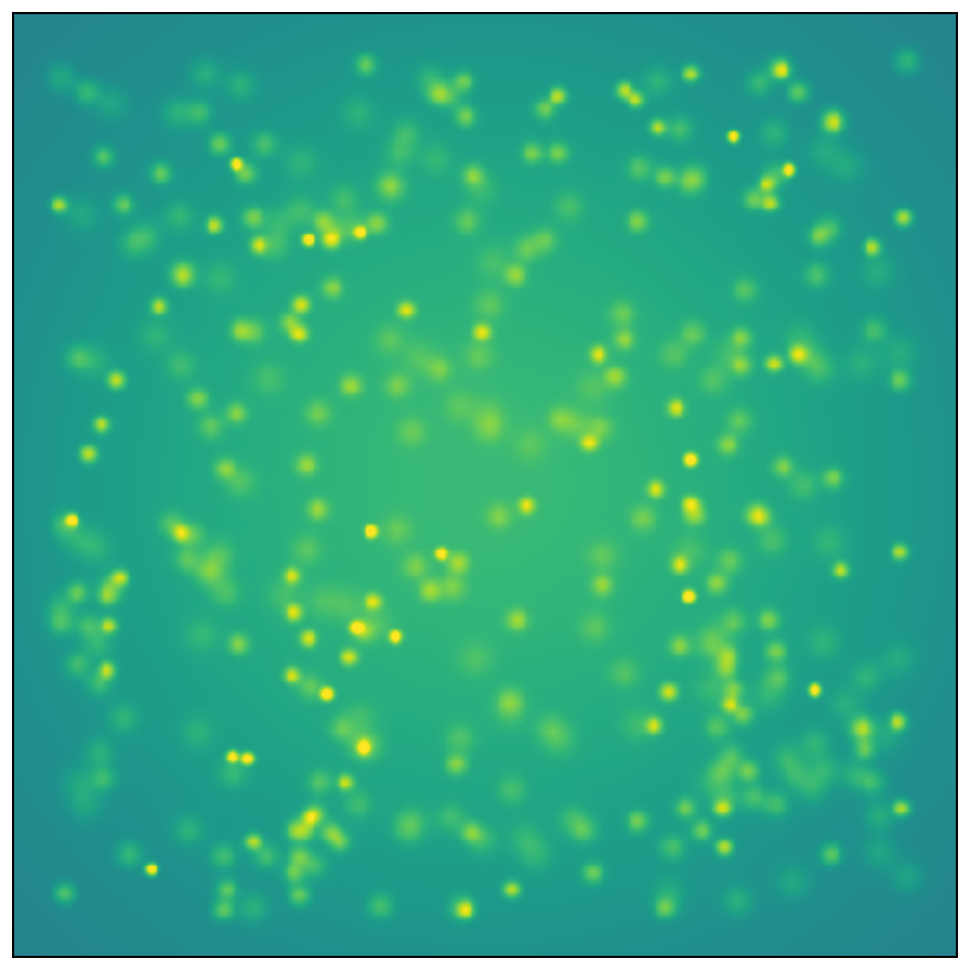
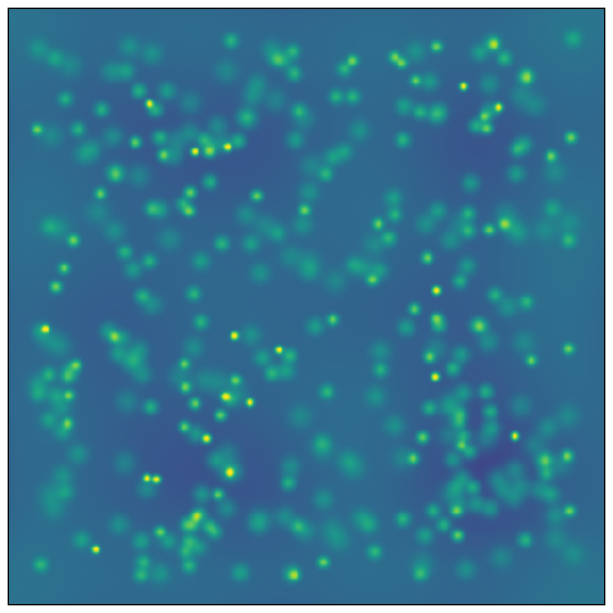
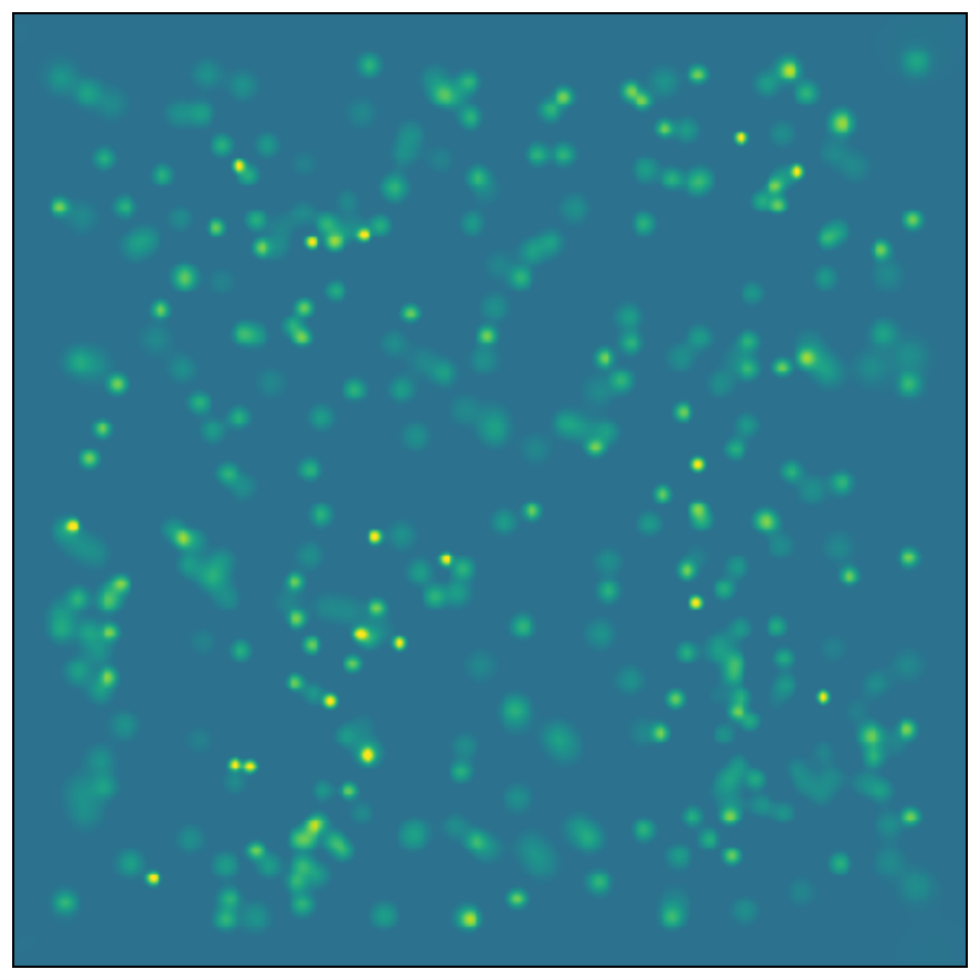
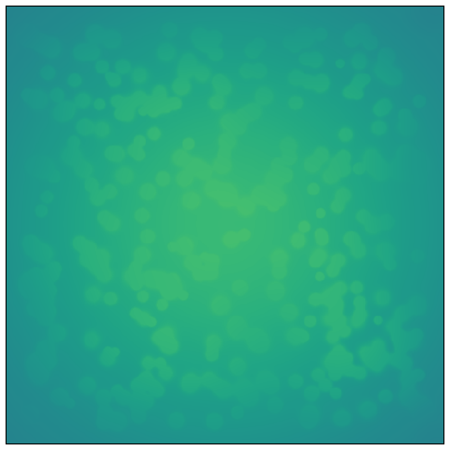
where is a post-processing mask applied to the result of the inverse Fourier transform (see Section 3.2) and is the filtered image with diffuse emission removed or reduced. An illustration of this process can be seen in Figure 1.


3.1 Filters
As a basis for describing frequency-based filters, we define two key quantities. Firstly, we define a distance for each component of the Fourier spectrum, in two-dimensional frequency space, from the zero-frequency ‘DC’ component:
| (5) |
Secondly, we define a critical distance in frequency space:
| (6) |
where is a physical size scale such that Fourier modes with wavelengths above this value are considered to be diffuse. We use the region separation length, , as measured by the Heisenberg code to define this distance. The filtering-to-region separation length scale ratio, , is a multiplicative factor of that softens the cut, reducing the value of and thus reducing the amount of attenuation from the filter. An illustration of its impact on the shape of a filter can be seen in Figure 2. Finally, is the length of one pixel in the same physical units as , where the pixels must be square.
We require a filter that removes diffuse emission while leaving the emission from the populations of interest (e.g. gas clouds and regions of star formation) intact. As these populations are compact, the Fourier transform of their emission will be concentrated in the low wavelength/high spatial-frequency part of Fourier space. Conversely, large scale diffuse emission, such as that from a sheet of gas or a galaxy scale Gaussian, will be primarily located in the high wavelength/low spatial-frequency part of Fourier space. For this reason, we only consider highpass filters, which allow high spatial frequencies to pass through the filter. We consider three different highpass filters:
- 1.
Ideal highpass filter
(7) - 2.
Gaussian highpass filter
(8) - 3.
Butterworth highpass filter
(9) with the Butterworth order .
A visual comparison of the Ideal, Gaussian, and Butterworth filters can be seen in Figure 3. For a given value of , the Ideal filter is the sharpest filter, fully attenuating frequencies lower than (the diffuse component) and allowing frequencies higher than (the compact component) to pass with no attenuation. On the other hand the Gaussian filter has a smoother roll-off and thus attenuates the compact part of frequency-space while not fully removing the diffuse part of frequency space. The Butterworth filter has a tunable sharpness that approaches a fully sharp Ideal filter as . However, the advantage, of smoother roll-off is that application of a smoother filter will create less ‘ringing’ or distortion in the resultant filtered image than a sharp filter does. We assess the suitability of these filters for use in filtering diffuse emission from input images for the Heisenberg code in Section 7.


3.2 Image post-processing
Due to the mathematical definition of the three highpass filters that we consider, the zero-frequency ‘DC’ component, which represents the mean flux of the image, is always set to zero (i.e. ). This necessarily results in a filtered image with zero mean flux and thus roughly zero total flux. As flux remains in the filtered image corresponding to the parts of frequency space that were unattenuated or partially attenuated by the filter, this leads to negative pixels in the filtered image. As we do not expect negative emission from a tracer map, this problem may be solved simply by applying a binary mask that sets all pixels to zero wherever the reverse Fourier transform is negative:
| (10) |
This results in a filtered image with a positive total flux. This is done in order to avoid an image with approximately zero flux after the removal of the ‘DC’ component. In the case where an image contains noise, this has the effect of biasing the image with positive noise flux. We investigate this effect in more detail in Appendix A.2.
3.3 Diffuse fraction measurement
The method that we employ to filter diffuse emission has the added benefit of decomposing an input tracer map into a map of compact emission and a map of diffuse emission. This allows us to quantify the fraction of emission within the map that is diffuse. The fraction of the flux in an image that is compact is simply the ratio of the total flux in the filtered (compact emission) image to the total flux in the original unfiltered image :
| (11) |
The relationship of to is described by equations 1 and 4. The diffuse fraction is then simply , as all flux must be either diffuse or compact. This gives us a physically motivated measure of the relative contribution of the diffuse and compact emission components in the tracer map. We use the cloud-separation length, , as the dividing line between diffuse and compact emission , with emission at spatial wavelengths greater than being diffuse emission and that at spatial wavelengths less than being compact emission. For example, in the case where is a tracer map of the molecular gas phase in a galaxy, the compact emission fraction represents the fraction of emission that comes from compact structures such as molecular clouds, whereas the diffuse fraction represents the fraction of the emission coming from large scale diffuse emission such as a reservoir of diffuse molecular gas or unresolved, low-mass molecular clouds.
4 Implementation within the Heisenberg code
We present a method, using iterative filtering in Fourier space, to remove diffuse emission present in tracer maps to be used with the Heisenberg code (Kruijssen et al. 2018b). As with the Heisenberg code, we have implemented this method in the Interactive Data Language (IDL)11 1 http://www.harrisgeospatial.com/SoftwareTechnology/IDL.aspx, in part using routines from the IDL Astronomy User’s Library22 2 https://idlastro.gsfc.nasa.gov/ and the IDL Coyote Library.33 3 http://www.idlcoyote.com/
A flowchart summarising the steps taken in the method can be seen in Figure 4. A user has two options of how to start the filtering process: they can either supply the original images alone, in which case Heisenberg is called to obtain a value for the initial calculation of ; or, if the user has calculated a value of externally, this value may also be supplied to the code for the initial calculation of , in which case the images are pre-filtered, before the first call to Heisenberg is made. After that, the Heisenberg code is fitted to the filtered maps, and a new value of and thus is calculated. The code then checks for convergence and either repeats the process of fitting Heisenberg in the case of no convergence or terminates and outputs the final values of all output parameters.

4.1 Input parameters
In order to run the presented method, a user has to specify a number of input flags, shown in Table 1, and input parameters, shown in Table 2, in addition to those flags and parameters described in Tables 1 and 2 of Kruijssen et al. 2018b.
Both the flags and input parameters are divided into two groups separated by white space. The first of these comprises flags and parameters added to Heisenberg itself and the second comprises flags and parameters that control the iterative diffuse filtering process. We consider most of these to be well described by reference to Tables 1 and 2. We provide some further explanation for some of the flags and parameters:
- 1.
If the flag peak_find_tui is set, the user is presented with a text-user-interface allowing them to adjust peak selection (see section 3.2.7 of Kruijssen et al. 2018b for details). The user is also presented with a DS9 window44 4 This optional feature requires the user to have the DS9 software package, which can be obtained from: http://ds9.si.edu, showing the input images with their identified peaks overlaid. The user may then adjust the parameters controlling peak selection through the text-user-interface and repeat the peak-finding process until they are satisfied with the identified peaks. This feature is of particular use during the iterative Fourier filtering process, as it allows the user to alter their peak selection parameters to adjust peak-finding after the removal of the diffuse background.
- 2.
Together, the parameters , a fractional tolerance between the measured value of in the current iteration and previous iteration and , the number of iterations over which the criterion should be satisfied, specify the iteration’s stopping condition:
(12) for . i.e. if the relative difference between value of calculated in the current iteration step and all values of calculated in the previous steps is less than , the iteration is considered to have converged and is terminated.
- 3.
In addition, sets the maximum number of iterative steps that will be taken ( + 1) before the code will terminate even if convergence has not been reached.
4.2 Code output
Each iterative step applies the Heisenberg code and the quantities described by Kruijssen et al. 2018b in their table 4 are measured and returned, in addition to the image compact emission fractions, as described in Table 3. The quantities are tracked and figures are made for the user showing how they change with each iterative step. Figure 5 shows examples of these figures for the fundamental physical quantities, , and , which are measured by Heisenberg. This allows the user to quickly visually inspect that convergence in the value of , on which the method’s iteration condition is based, has also resulted in satisfactory convergence of the other quantities. In addition, the filtered map (of compact emission) and the diffuse emission map produced in each step are saved to disk. This makes these maps available for further analysis on the two components and allows the user to visually inspect the filtered map for distortions. An example of these maps can be seen in panels e and f of Figure 1.


| Flag | Values (default) | Description |
|---|---|---|
| diffuse_frac | 0/1 | Calculate diffuse fraction in images (off/on) |
| peak_find_tui | 0/1 | Use interactive peak identification interface to refine initial peak selection (off/on) |
| f_filter_type | 0 | Use an Ideal filter for the determination of diffuse fractions (see equation 7) |
| 1 | Use a Gaussian filter for the determination of diffuse fractions (see equation 8) | |
| 2 | Use a Butterworth filter for the determination of diffuse fractions (see equation 9) | |
| use_sds | 0 | Automatically calculate map sensitivity limits as described in section 3.2.6 of Kruijssen et al. 2018b |
| 1 | Pass in externally calculated values of map sensitivity limits to the code | |
| use_guess | 0 | Calculate for the first filtering step by fitting Heisenberg to the unfiltered maps (option 1 in Figure 4) |
| 1 | Use an initial estimated value of to determine for the first filtering step (option 2 in Figure 4) |
| Parameter | Default | Description |
|---|---|---|
| 2 | The order of the Butterworth filter used to calculate map diffuse fractions (only used if f_filter_type = 0) | |
| 1.0 | Multiplicative factor used in calculating map diffuse fractions for calculating that reduces filter attenuation for a given value of (see equation 6) | |
| - | The measured sensitivity limit of the star formation tracer map in units of the map | |
| - | The measured sensitivity limit of the gas tracer map in units of the map | |
| - | Length in pc of the initial estimate of lambda (only used if use_guess = 1) | |
| 0.05 | Maximum fractional difference between and previous value(s) that triggers the iteration process to terminate | |
| 2 | Number of steps over which the iteration criterion, , must be true for iteration to terminate | |
| 10 | Maximum number of steps in the iterative diffuse filtering process, before the iteration is terminated | |
| 2 | The order of the Butterworth filter used in the iterative diffuse filtering process (only relevant if f_filter_type = 0 ) | |
| 1.0 | Multiplicative factor used in the iterative diffuse filtering process for calculating that reduces filter attenuation for a given value of (see equation 6) |
| Quantity | Equation | Description |
|---|---|---|
| 11 | The fraction of emission in the stellar tracer map that is not diffuse | |
| 11 | The fraction of emission in the gas tracer map that is not diffuse | |
| 30 | The relative flux loss from compact stellar regions due to filtering in Fourier space (see Section 6) | |
| 30 | The relative flux loss from compact gas regions due to filtering in Fourier space (see Section 6) | |
| 32 | The evolutionary phase lifetime adjusted star formation filling factor (see Section 6) | |
| 33 | The evolutionary phase lifetime adjusted gas filling factor (see Section 6) | |
| 34 | The relative flux loss from stellar regions due to overlap between regions in the stellar map (see Section 6) | |
| 34 | The relative flux loss from gas regions due to overlap between regions in the gas map (see Section 6) |
5 Generation of test images
In order to test and validate the presented iterative diffuse filtering method we generate test input datasets. Each test dataset consists of a pair of test images, of size , such that both images in the pair are square and of the same size. We note that these choices are made for simplicity and are not restrictions of the method. Each image is made up of two components: a compact component and a background component :
| (13) |
An example image generated in this manner is shown in Figure 6.


5.1 The signal component
For the Heisenberg code to be applied we require two maps: one representing a progenitor phase and one representing a descendent phase in an evolutionary sequence. In order to create the compact component for these maps, we generate three compact populations: a population that is visible only in the progenitor map, one that is visible only in the descendant map and an ‘overlap’ population that is visible in both maps. Hereafter, we will assume that our progenitor population is made up of gas clouds and that our descendent population is made up of young stellar regions (Hii regions) and thus refer to them as ‘gas’ and ‘stars’. In this scenario, our overlap population represents the phase of star formation where young stars have been formed and are still co-spatial with their natal cloud. This is the phase during which feedback operates to eventually cause the cloud to cease be visible in the gas tracer map (for example through photodissociation or physical transportation of the gas away from the young stars). We note, however, that the Heisenberg code may be applied applied more generally, to any scenario characterised characterised by an evolution from a population visible in one tracer map to a descendent population visible in another tracer map. Likewise, the presented method of removing diffuse emission from a tracer map may be used in other situations, in which one wishes to remove an extended diffuse component from a tracer map containing both this diffuse component and a population of compact regions.
To simulate the gas, stellar and overlap populations, we generate Gaussian functions and position them randomly within our maps. We determine the position of the central pixel of the Gaussian function by drawing random numbers from a uniform distribution:
| (14) |
| (15) |
We set the characteristics of the compact component with the following parameters: , the number of Gaussian functions appearing in the gas map only; , the number of Gaussian functions appearing in the stellar map only; , the number of peaks appearing in both the gas and stellar maps; and and , the full width at half maximum (FWHM) of the Gaussian functions seeded into the stellar and gas maps, respectively. We consider a number of different models for the FWHMs of the regions:
- 1.
Uniform FWHM model:
In this model, all the Gaussian regions in each pair (stellar and gas) of images have the same FWHM:(16) where is a uniform random number chosen for each experiment such that . In this model, the total flux of each region is equal to that of each other region.
- 2.
Asymmetric uniform FWHM model:
In this model, we set a common FWHM value for all Gaussian regions in the stellar map, and another one for all the Gaussian regions in the gas map:(17) (18) where and are individually chosen uniform random numbers chosen for each experiment such that and .As with the previous model, the flux of each region is equal to that of each other region.
- 3.
FWHM spread model:
In this model, each individual Gaussian region in the stellar and gas maps has a randomly selected FWHM, selected within the same range of values for both maps(19) (20) As with the previous models, the flux of each region is equal to that of the other regions, irrespective of the randomly selected FWHM of a region.
- 4.
FWHM flux spread model:
The FWHM of regions in this model is selected in the same way as the ‘FWHM spread model’ (i.e. according to equations 19 and 20). However, in this model the flux of regions are not equal to that of each other region, instead the flux of a region is proportional to its size, i.e. .
For each of these models, regions in the overlap phase are selected from the same size distribution as the gas and stellar regions. For the asymmetric uniform FWHM model, an overlap region has size in the stellar map and size in the gas map.
In order to test the effectiveness of the method, we compare measured values of the three key quantities measured by the Heisenberg code (the gas cloud lifetime, , the overlap phase lifetime, , and the mean separation length between regions, ; recall that the young stellar lifetime is assumed to be known a priori) to values known from the generation of the test datasets. The relative visibility lifetimes of each population are linked to the relative number of regions in each population. Therefore, for and in relation to we have:
| (21) |
and
| (22) |
where is used as the reference time-scale. As we are not directly simulating a particular tracer, the actual value of the reference time-scale is not relevant. We choose , which is close to typical values found for visibility lifetimes of star formation tracers by Haydon et al. 2018.
For each image, we select a value of the filling factor, , the region size-to-mean separation ratio. Given our selected value of and , we calculate a value of the mean separation length between regions, , following the definition of in equations 136 and 137 in Kruijssen et al. 2018b, which we reproduce here:
| (23) |
| (24) |
where from the original definition in Kruijssen et al. 2018b. This filing factor represents the amount of blending between peaks and is a key quantity in determining the applicability of the Heisenberg code. Testing performed by Kruijssen et al. 2018b shows that the quality of measurements obtained declines as increases above . We will therefore assess the quality of the presented diffuse filtering method at different filling factors based on that criterion.
Lastly, we determine the number of pixels, , of the image to be generated, by using the total number of peaks in the image set, the mean separation length, , and the pixel length scale, :
| (25) |
where . As must be an integer number, this calculation introduces a small rounding error. We therefore recalculate the effective value of from the definition of the geometric mean separation length for the total number of regions in the total area of a map (Kruijssen & Longmore 2014, appendix A2 of), which in practice is an inversion of equation (25).
.
| Value range | |||||
| Parameter | points | Gaussians | Main set 1 | Main set 2 | Origin |
| N/Aa | input | ||||
| N/Aa | a | b | b | input | |
| input | |||||
| input | |||||
| input | |||||
| input | |||||
| 10 | 10 | 10 | 10 | Equation 21 | |
| 10 | Equation 21 | ||||
| Equation 22 | |||||
| b,c | b | b | b | Equation 23 | |
a The definitions of and do not apply to single pixel regions
b For all quantities in units of we have applied a pixel length scale of
c For images containing point sources, we calculate lambda with equation 25 by specifying the image size
5.2 The background component
We consider a number of different models of the diffuse background, with increasing levels of complexity:
- 1.
Constant background:
The simplest model that we consider is that of a spatially uniform constant diffuse background:(26) with selected such that the fraction of the diffuse background may vary in significance relative to the compact component.
- 2.
Extended Gaussian and constant background:
This background model consists of both a constant background and a large ‘galaxy-scale’ Gaussian function.(27) with the normalisation factors, and varying such that the two components may vary in significance in relation to each other and that the significance of the background component may vary relative to the compact component. The FWHM of the ‘galaxy-scale’ Gaussian, , is chosen such that so as to represent a large galactic background that decreases smoothly with radius.
- 3.
Envelopes, Extended Gaussian and constant background:
In addition to the constant and galaxy scale Gaussian background, this background model includes Gaussian envelopes with centres co-spatial to the compact Gaussian regions seeded into the maps. The FWHM of the envelopes is set to be a multiple of the region separation length, , where we consider . As with the previous models, the normalisation of each of the components is randomly chosen for each experiment such that the significance of each component varies and the significance of the total background varies in relation to the compact component.
The true value of the compact emission fraction () in an image is calculated as the total flux in the compact component divided by the total flux in the image (including the background component):
| (28) |
Overlap between regions causes flux loss from compact regions after the application of Fourier filtering. In Section 6, we use the method presented here to generate simulated datasets to investigate this effect. In Section 7, we again use the method to generate datasets to evaluate the performance of the method at removing diffuse emission. A summary of the parameter spaces used for each each section is presented in Table 2.
6 The impact of filtering on signal regions
The value of given by equation 11 assumes that filtering removes none of the flux of the compact regions. However, the flux from a Gaussian region is spread out in Fourier space, such that the application of a filter in Fourier space removes some of the flux from compact regions. This flux loss should be quantified, so that it can be corrected for.
6.1 Flux loss for a single Gaussian region
We define the fraction of flux remaining in an image containing a single Gaussian function after filtering as:
| (29) |
Figure 7 shows after the application of Gaussian filters, where is set with variable values of . For the smallest, pixel region, which we do not show, we do not see a smooth function between the flux fraction and critical filter length-scale, as the function is insufficiently resolved.
In the right-hand panel of Figure 7, we see that can be well fitted by a simple analytical function of the relative width of the Gaussian filter over the width of the compact regions, , for all the Gaussian functions with pixels.


By again plotting against for the other considered filters, the Ideal filter and Butterworth filters, we obtain relationships of varying quality, which are shown in Figure 8. We again find the smallest ( pixel) Gaussian functions to be insufficiently resolved and thus we impose the condition that the FWHM of the Gaussian regions in the image pixels for the successful application of the method. While the remaining flux fraction is strictly less than or equal to unity after the application of the Gaussian filter, it is above one (even up to ) in some cases after the application of the Ideal filter, due to the significant distortions introduced into the image. For this reason, we discard the Ideal filter from further consideration. The Butterworth filter is tunable, where at low values of the filter is smooth, akin to the Gaussian filter, but becomes sharper, approaching an Ideal filter as . For the 1st order Butterworth filter, we again obtain a simple analytical function, where . For , however, we see that is greater than 1 in some instances, with the magnitude of the effect greater as increases.
We fit a sigmoidal function for , as a function of :
| (30) |
where we set for all filters, so that as , , as this represents 0% flux loss from the Gaussian region in the image. The value of sets the zero point of the function, such that for . The value of sets the steepness of the transition between and , with higher values of representing a steeper transition. The value of is the value of at which . The best fitting values of these parameters are shown in Table 5 and a comparison of the fitted functions is shown in Figure 9.
We first compare the Gaussian and 1st order Butterworth filters, which both have the property that the flux remaining after their application in the single Gaussian region is strictly less than or equal to 100% of the original flux. Between the two, the Gaussian filter offers a steeper response curve that removes less flux from the compact regions than the 1st order Butterworth filter. Butterworth filters of 2nd order and greater offer a significantly steeper response curve than the Gaussian filter and thus remove less flux from the compact regions than the Gaussian filter. However, due to introduced distortions, application of the filter does not necessarily result in an image that has of the flux of the original image. As the Gaussian filter shows few distortions we chose to focus on this filter for the remainder of our analysis.
We can now correct the measured value of for the lost emission from a single Gaussian region as follows:
| (31) |
| Parameter | Gaussian | 1st order BW | 2nd order BW |
|---|---|---|---|
BW = Butterworth
6.2 Flux loss for a set of overlapping Gaussian regions
Astronomical images do not consist of only single isolated Gaussian functions. Instead, there are a number of overlapping regions distributed within each image. As Figure 10 demonstrates, in the case of an image made up of a field of multiple Gaussian functions, we no longer recover a simple analytical relationship between the remaining flux fraction, , and . We can characterise the effect of overlap between regions in terms of in terms of the the evolutionary phase lifetime adjusted filling factor, , which we define as:
| (32) |
for the stellar map, and
| (33) |
for the gas map, where is the total duration of evolutionary timeline. Thus, is given by the global filling factor, ,55 5 For the definition of this filling factor, see Equations 23 and 24. multiplied by and for the stellar and gas maps, respectively, in order to weight the global filling factor by the number of regions in each of the two tracer maps, as expected from the evolutionary timeline.


We generate a set of simulated datasets with single pixel compact regions and a constant background to serve as a control dataset (‘ points’). As point sources are not extended in space, we expect no flux loss from the compact regions after the application of a filter in Fourier space (i.e. and ). For Gaussian compact regions (‘ Gaussians’), we do expect flux loss due to overlapping regions. For all of these datasets, we set . Detailed testing of the Heisenberg by Kruijssen et al. 2018b shows that the condition should be satisfied for accurate measurements to be obtained from the code and that the Heisenberg code produces better results the lower the value of is. As we will use this dataset to fit for an empirical relationship between and , we ensure good performance by considering a restricted range of , i.e. 10-50 and a range of values of up to the maximum recommended value. (i.e. ). A summary of the parameters used to generate these datasets is given in Table 4. The value of is randomly selected to be between 15% and 100% of the total flux in each image. For a full description of the method used to generate these images see Section 5.
Figure 11 shows the measured value of the image compact emission fraction against the true compact emission fraction, measured according to equation 11 with the application of Gaussian filters with varying values of . This figure illustrates how, for images where the compact regions are single pixels, the true value of the compact emission fraction is recovered with equation 11. However, for those images where the compact regions are extended Gaussians, the true value is not accurately recovered.
We correct these measurements for the flux loss from a single Gaussian, . The resulting measurements of (according to Equation 31) are shown in Figure 12 as a function of . It can be seen that, while the spread in measured values has been greatly reduced, we do not yet recover the true values of and that decreases with increasing .
We then calibrate an empirical relationship between and the ratio of the measured flux fraction to the true flux fraction, after the flux fraction has been corrected for the flux lost from a single Gaussian region. We adopt a critical value of , because, as can be seen in the right hand panel of Figure 7, a small uncertainty in the measurement of leads to a small uncertainty in the measured value of above this threshold. By contrast, a small measurement uncertainty in below this threshold leads to a large uncertainty in , making this correction unreliable. Indeed, the experiments with display a clear relation with in Figure 12, because they represent cases for which a small fraction of the compact emission is filtered out. We fit a linear relationship between the flux loss due to overlap, , and the evolutionary timeline normalised filling factor, , truncated such that may never be greater than unity:
| (34) |
The best-fitting slope and intercept for the Gaussian filter is listed in Table 6 and is plotted in Figure 12.
| Parameter | Gaussian |
|---|---|
| A | |
| B |
Thus applying this empirical correction in addition to the correction for the flux lost from a single Gaussian region, the final measurement of the compact emission fraction, , in an image, is:
| (35) |
The original measurements shown in Figure 11 are shown with these corrections applied in Figure 13. The true value of is then recovered, with some scatter for those cases where . For cases where , the upward scatter on the measured value of increases, biasing the measurement. For this reason we recommend the choice of the filtering-to-region separation length scale ratio, , such that . We can quantify this recommendation for in terms of the map filling factor, , by substituting equations 23 and 24 into equation 30 for and rearranging for :
| (36) |
where is the maximal filling factor for the pair of gas and stellar maps. For the Gaussian filter (values of the fitting parameters, , and are shown in Table 5) at the maximally recommended value of the filling factor (, from testing by Kruijssen et al. 2018b) and given our recommendation that we would therefore recommend . For a lower value of the filling factor () this equation implies a recommendation of , allowing much tighter filtering. In the case that one wishes to filter out wavelengths shorter than allowed given these recommendations, a sharper filter, such as a second order Butterworth filter may be considered.
7 Testing and validation
We now test the performance of the method at separating diffuse and compact emission in the generated images. We test this performance with regards to the recovered values of the three key fitting parameters of the Heisenberg code: the gas cloud lifetime, , the region overlap timescale, , and the mean separation length , and the image compact emission fraction, .
We test the method on two test datasets, ‘Main set 1’, for short to intermediate values of and ‘Main set 2’, for intermediate to long values of . We make this division for computational reasons. In our simulated datasets, increasing the value of leads to an increase in the size of the maps in the datasets (see Equation 25). In order to run datasets with large values of in a reasonable time, we reduce the number of Gaussian regions seeded into our reference stellar map (see Table 2) and thus the required number of Gaussian regions in the gas maps, leading to a reduction in the overall size of the maps. For these datasets, we set the reference timescale to (i.e. ). We consider a range of between 5 and 100 (i.e. ). For , the range of possible values for a dataset is between 0 and the minimum of and (i.e. ). Initial applications of Heisenberg to nearby galaxies that are currently being undertaken (Kruijssen et al. 2018a; Hygate et al. 2018; Chevance et al. 2018; Ward et al. 2018) have measured values of between and . We will thus consider values of over a suitable range (i.e. and ). We note, however, that detailed testing of the Heisenberg by Kruijssen et al. 2018b shows that the condition should be satisfied for good performance of the Heisenberg code. For this reason, we focus our analysis on those experiments with , keeping experiments with = 0.5 as borderline cases.
Together, the selected evolutionary timelines and values of translate to a range of between 55 for datasets with the highest value of the filling factor (), and 420 for datasets with the lowest value of the filling factor (). For all images, the compact emission fraction, , can vary between 10% and 100%. For each combination of compact region model (detailed in Section 5.1) and diffuse model (detailed in Section 5.2) and each considered value of the filling factor, , we generate 100 experiment datasets (50 each for main dataset 1 and main dataset 2).66 6 For , this equates to 200 measurements per combination as we make a measurement of the compact fraction in the stellar map and the gas map of each experiment dataset. For main dataset 1 and main dataset 2, we generate 50 gas and stellar map pairs, for each combination of compact region model and each considered value of the filling factor, . We remove experiments with obviously visibly bad fits from the datasets with between 0.2 and 0.5. This concerns 116 out 6400 experiments ( of the experiments).
This equates to a total of 100 experiments for each combination .77 7 For , this equates to 200 measurements per combination as we make a measurement of the compact fraction in the stellar map and the gas map of each experiment map pair. For each map pair, we select a randomised evolutionary timeline, where may vary between 5 and 100 (i.e. ) and may vary between 0 and the minimum of and (i.e. ). The value of is randomly selected to be between 10% and 100% of the total flux of the image. For full details on the generation of experiment datasets see Section 5 and for the full set of parameters used in this generation see Table 4.
A summary of the measured quantities for these experiments, both before and after filtering, is shown in Figure 14 for , and and in Figure 15, for . Experiments with unsatisfactory values of the filing factor () are shown as grey hexagons and those with satisfactory filling factor () are shown as coloured symbols. A key to the plotting symbols used for each combination of compact and diffuse model is shown in Table 7. A summary of the measured quantities for these experiments, both before and after filtering, is shown in Figure 14 for , and and in Figure 15, for .
| Diffuse Model | ||||
|---|---|---|---|---|
| Compact Model | none | constant | large Gaussian | envelopes |
| Uniform FWHM | ||||
| Asymmetric FWHM | ||||
| Spread FWHM | ||||
| Flux spread FWHM | ||||
Experiments with unsatisfactory filling factor () are displayed as grey hexagons () regardless of the combination of diffuse and compact model
For experiments with no added diffuse reservoir, we recover values of these quantities close to the correct values both before and after Fourier filtering. For this is unity, due to there being no diffuse reservoir in the images. This indicates that the distortions introduced into the images do not significantly affect the total flux of the image or the correct identification of peaks (i.e. only few spurious peaks are introduced into the image by filtering) and thus in turn the measurement of these quantities. However, the addition of diffuse reservoirs does significantly affect the measured values of the quantities in the unfiltered images. After Fourier filtering, and the removal of the diffuse reservoir, we again measure values of these quantities that are close to the true values. The distribution of the recovered quantities is also not significantly different between experiments with added diffuse emission and without, with the exception of the measured compact emission fraction, which is for all the experiments without an added diffuse background.
We do find a number of other elements that can bias the measurements. For instance, as increases, the measurement of worsens, as described in Kruijssen et al. 2018b. For , we note that the line of points in the middle left panel in Figure 14 (at ) is due to the fact that in all cases , because it is physically impossible for regions to coexist with other regions for a time longer than their own lifetime (and for all of our experiments).88 8 In a minority of experiments, is shorter than . In this case, sets the upper limit for
For , we note that our prediction, as given in equation 25, systematically overestimates the values measured in our experiments, by (see the bottom right panel of Figure 14). As there is no significant offset between the values of measured for experiments without added diffuse emission both before and after filtering we conclude that this is not an offset introduced by Fourier filtering. Instead this discrepancy is due to the geometric mean separation between regions that we calculate being an overestimate of the actual local mean separation of the regions. After all, the scatter introduced by the random positioning of the peaks causes them more often than not to be positioned closer to their near neighbours than the geometric mean separation length. This slight overestimation of propagates into a corresponding, minor underestimation of the compact emission fraction in Figure 15.
For those datasets with unsatisfactory values of the filling factor (i.e. ), indicated as grey hexagons in Figures 14 and 15, the accuracy of the measurements decreases for larger values of . As the amount of blending in an individual tracer map ( and , see Equations 32 and 33) scales with the lifetime of that particular tracer in units of the total duration of the timeline, the effect of blending in both maps is roughly equal when . However, as increases, increases too (while decreases due to the increase of the total duration of the timeline), leading to more severe blending in the gas map and more inaccurate results overall.
In summary, we see that the filtering method performs well regardless of the compact region model used, with no significant difference between the scatter of measured values between the different models after filtering. With respect to the diffuse background models, successful filtering of the constant diffuse model and the Gaussian diffuse model is relatively insensitive to the value of the filtering-to-region separation length scale ratio, , chosen, due to the fact that a constant sheet of diffuse gas and a galaxy-scale Gaussian correspond to infinite and very large spatial wavelengths, respectively, whereas is typically much smaller than a galactic radius. Galaxies with radii have a typical region separation length (as measured from initial applications of the method: Kruijssen et al. 2018a; Hygate et al. 2018; Chevance et al. 2018; and Ward et al. 2018), giving a factor of in size between the two. Thus the value of selected is relatively unimportant with regards to the filtering of galactic-scale components of diffuse emission. By contrast, the envelope diffuse model requires filtering with lower values of , because the modelled envelopes are much closer in size to . Figure 16 shows how the performance of the method at removing each of these diffuse models varies with the chosen value of . This summarises the above discussion, i.e. the value of does not affect the filtering of galactic-scale emission, but in order to accurately filter diffuse envelopes of regions, we require . The criterion is easily satisfied, as in practice one would expect and the resulting is a very generous condition.
Overall, we are able to accurately constrain the cloud lifecycle ( and ), the cloud separation length () and the diffuse and compact emission fractions after filtering the diffuse emission in Fourier space, regardless of the significance of the added diffuse emission. We are able to do this for all of the compact region models and diffuse emission region models that we consider.


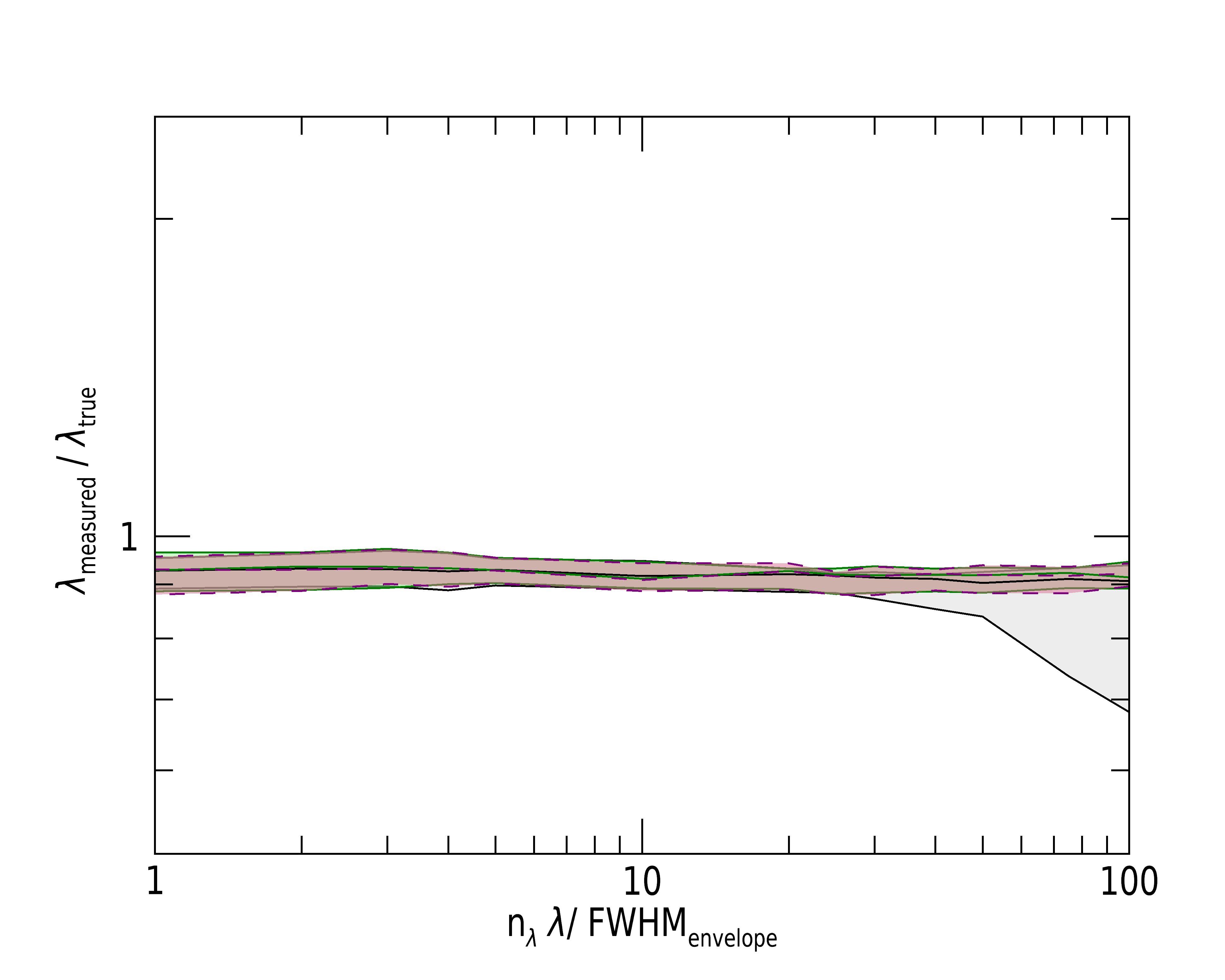
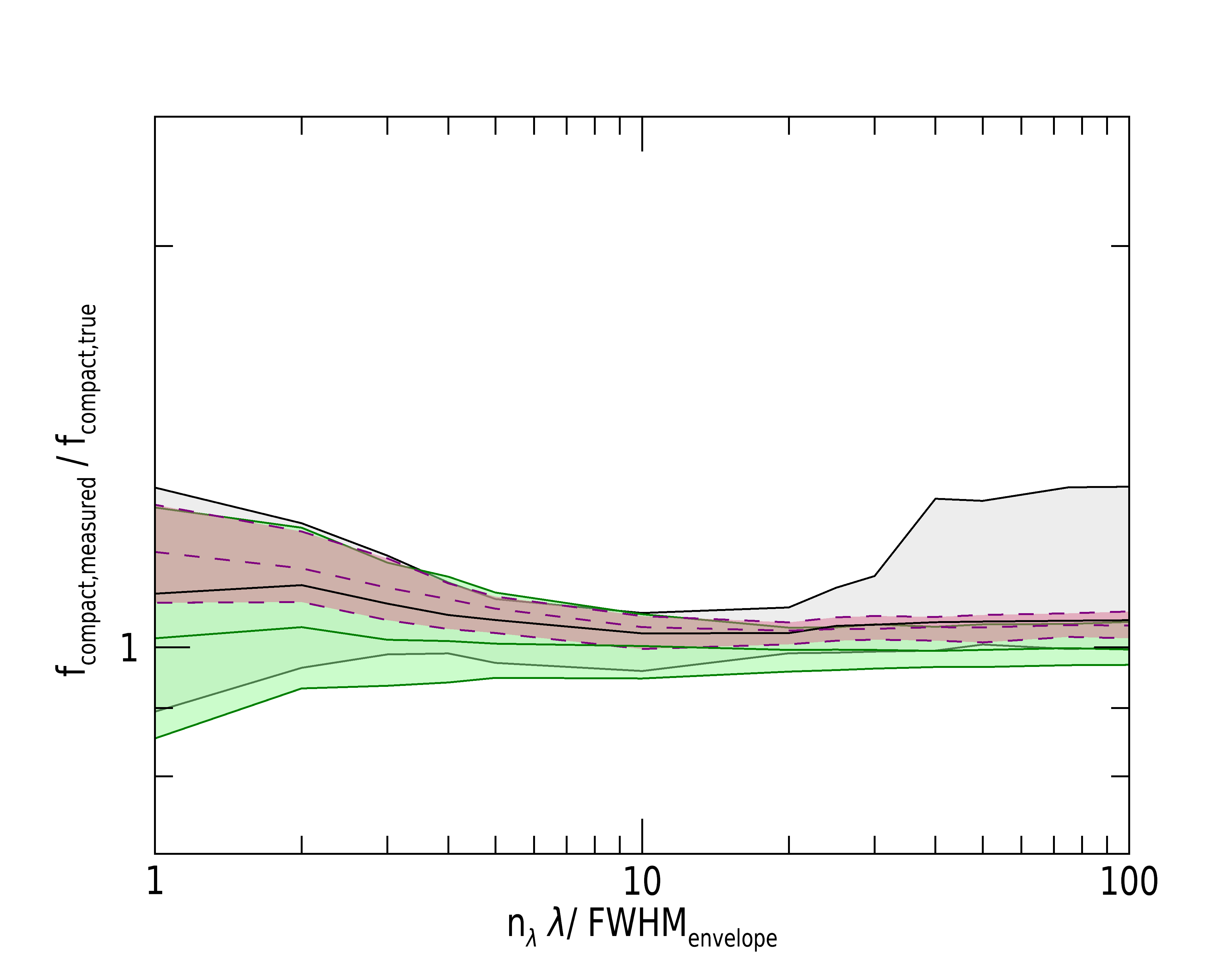
Finally, we note that the results presented in this section are based upon idealised datasets that contain no noise and are perfectly aligned in astrometry. In reality tracer maps will contain observational noise and two different tracer maps may be astrometrically offset from each other. We detail the impact that these two observational limitations have on the method in Appendix A. In Appendix A.1, we show that astronometric uncertainty less than one third compact region FWHM (i.e ) must be achieved for meaningful constraints of and in Appendix A.2 we show that the use of low or intermediate signal to noise data will lead to biased results, unless a method to reduce the noise is used.
8 Conclusions
We have presented a physically motivated method for the filtering and measurement of diffuse emission (such as the diffuse Warm Ionised Medium that is observed in H along with compact Hii regions) in images by filtering in Fourier space. We have validated our method’s performance within the Heisenberg code (Kruijssen et al. 2018b) by testing for the accurate recovery of the three key fitting-parameters measured by the Heisenberg code (, and ). These tests are based on a range of models of compact regions and diffuse backgrounds, as detailed in Section 5. We demonstrate that the presence of diffuse emission can have a significant impact on the measurement of the measured cloud-scale quantities, but also demonstrate that our filtering method accurately alleviates this problem. A summary of these tests can be seen in Figure 14. We have also validated its performance for measuring the fractions of diffuse and compact emission within tracer maps, which is summarised in Figure 15. Finally, we report a number of criteria that need to be satisfied for the reliable application of the method, which we summarise here:
- •
The observed compact regions need to be sufficiently resolved ( pixels) or to be point sources.
- •
The value of the filtering-to-region separation length scale ratio, , should be chosen such that the flux-loss from compact regions due to the application of the Fourier filter is minimised, i.e. .
- •
For meaningful constraints on the value of , the astrometric uncertainty between images should be less than one third the FWHM of the regions of interest (i.e ), see Appendix A.1.
- •
In the case of low or intermediate signal to noise, the presence of noise will lead to biased results unless a noise-reduction method is employed such as lowpass Fourier filtering (See Appendix A.2).
We also note that common reduction techniques for astronomical data may reduce the amount of diffuse emission present in a tracer map. For example, the practice of filtering molecular gas tracer maps to exclude emission that is not associated in velocity space with HI emission (see Gratier et al. 2010) may remove some fraction of the diffuse emission from the final tracer map, depending on the filtering parameters chosen for this reduction process. The presented method will only measure the fraction of diffuse emission remaining in the map presented to it after any prior reduction process is complete.
In conclusion, we have demonstrated how, by filtering in Fourier space using the mean region separation length, , we can remove diffuse emission from tracer images. This allows the Heisenberg code to be applied to observationally constrain cloud scale ISM physics, such as cloud lifecycles, without the biasing impact of diffuse emission. In addition, by separating the diffuse and the compact emission within the images, we are able to measure their relative contribution to the total emission within the images. The method also produces maps of the compact and diffuse emission within each input tracer map that may be used for further analysis such as investigating spatial variations in the diffuse emission fraction within galaxies. This approach will provide critical astrophysical constraints on e.g. the unresolved population of low-mass GMCs, and the ionised photon escape fraction.
Acknowledgements
APSH and DTH are fellows of the International Max Planck Research School for Astronomy and Cosmic Physics at the University of Heidelberg (IMPRS-HD). JMDK and MC gratefully acknowledge funding from the German Research Foundation (DFG) in the form of an Emmy Noether Research Group (grant number KR4801/1-1). JMDK gratefully acknowledges funding from the European Research Council (ERC) under the European Union’s Horizon 2020 research and innovation programme via the ERC Starting Grant MUSTANG (grant agreement number 714907). APSH warmly thanks Fabian Walter for extensive discussions on the content of this work, as well as more broadly on interferometric techniques.
References
- Baldwin et al. (1981) Baldwin J. A., Phillips M. M., Terlevich R., 1981, PASP, 93, 5
- Blanc et al. (2009) Blanc G. A., Heiderman A., Gebhardt K., Evans II N. J., Adams J., 2009, ApJ, 704, 842
- Bregman & Pildis (1994) Bregman J. N., Pildis R. A., 1994, ApJ, 420, 570
- Caldú-Primo et al. (2013) Caldú-Primo A., Schruba A., Walter F., Leroy A., Sandstrom K., de Blok W. J. G., Ianjamasimanana R., Mogotsi K. M., 2013, AJ, 146, 150
- Caldú-Primo et al. (2015) Caldú-Primo A., Schruba A., Walter F., Leroy A., Bolatto A. D., Vogel S., 2015, AJ, 149, 76
- Chevance et al. (2018) Chevance M., et al., 2018, to be submitted
- Crocker et al. (2013) Crocker A. F., et al., 2013, ApJ, 762, 79
- Dettmar (1990) Dettmar R.-J., 1990, A&A, 232, L15
- Fabbiano et al. (1990) Fabbiano G., Heckman T., Keel W. C., 1990, ApJ, 355, 442
- Gratier et al. (2010) Gratier P., Braine J., Rodriguez-Fernandez N. J., Israel F. P., Schuster K. F., Brouillet N., Gardan E., 2010, A&A, 512, A68
- Haydon et al. (2018) Haydon D. T., Kruijssen J. M. D., Longmore S. N., 2018, MNRAS to be submitted
- Hoopes et al. (2001) Hoopes C. G., Walterbos R. A. M., Bothun G. D., 2001, ApJ, 559, 878
- Hygate et al. (2018) Hygate A. P. S., Kruijssen J. M. D., Walter F., Chevance M., Schruba A., Longmore S. N., Haydon D. T., 2018, to be submitted
- Kapala et al. (2015) Kapala M. J., et al., 2015, ApJ, 798, 24
- Kreckel et al. (2016) Kreckel K., Blanc G. A., Schinnerer E., Groves B., Adamo A., Hughes A., Meidt S., 2016, ApJ, 827, 103
- Kruijssen & Longmore (2014) Kruijssen J. M. D., Longmore S. N., 2014, MNRAS, 439, 3239
- Kruijssen et al. (2018a) Kruijssen J. M. D., et al., 2018a, submitted
- Kruijssen et al. (2018b) Kruijssen J. M. D., Schruba A., Hygate A. P. S., Hu C.-Y., Haydon D. T., Longmore S. N., 2018b, MNRAS, 479, 1866
- Lacerda et al. (2018) Lacerda E. A. D., et al., 2018, MNRAS, 474, 3727
- Leroy et al. (2012) Leroy A. K., et al., 2012, AJ, 144, 3
- Liu et al. (2011) Liu G., Koda J., Calzetti D., Fukuhara M., Momose R., 2011, ApJ, 735, 63
- Mathis (1986) Mathis J. S., 1986, ApJ, 301, 423
- Monnet (1971) Monnet G., 1971, A&A, 12, 379
- Oey et al. (2007) Oey M. S., et al., 2007, ApJ, 661, 801
- Pety et al. (2013) Pety J., et al., 2013, ApJ, 779, 43
- Rand et al. (1990) Rand R. J., Kulkarni S. R., Hester J. J., 1990, ApJ, 352, L1
- Reynolds et al. (1973) Reynolds R. J., Scherb F., Roesler F. L., 1973, ApJ, 185, 869
- Sembach et al. (2000) Sembach K. R., Howk J. C., Ryans R. S. I., Keenan F. P., 2000, ApJ, 528, 310
- Seon & Witt (2012) Seon K.-I., Witt A. N., 2012, ApJ, 758, 109
- Strickland et al. (2004) Strickland D. K., Heckman T. M., Colbert E. J. M., Hoopes C. G., Weaver K. A., 2004, ApJS, 151, 193
- Thilker et al. (2000) Thilker D. A., Braun R., Walterbos R. A. M., 2000, AJ, 120, 3070
- Thilker et al. (2002) Thilker D. A., Walterbos R. A. M., Braun R., Hoopes C. G., 2002, AJ, 124, 3118
- Thilker et al. (2005) Thilker D. A., et al., 2005, ApJ, 619, L67
- Ward et al. (2018) Ward J. L., Kruijssen J. M. D., Chevance M., Hygate A. P. S., Schruba A., Longmore S. N., 2018, to be submitted
- Wilson & Walker (1994) Wilson C. D., Walker C. E., 1994, ApJ, 432, 148
- Wood et al. (2010) Wood K., Hill A. S., Joung M. R., Mac Low M.-M., Benjamin R. A., Haffner L. M., Reynolds R. J., Madsen G. J., 2010, ApJ, 721, 1397
- Zhang et al. (2017) Zhang K., et al., 2017, MNRAS, 466, 3217
Appendix A Observational Considerations
For the main body of the paper, we have tested diffuse emission filtering in Fourier space on idealised simulated datasets. In this appendix, we consider the impact of two features of astronomical observations on the validity of the method. We firstly consider the impact of astrometric offsets between two input images and then we consider the impact of noise in images.
A.1 Systematic astrometric offsets
One issue that impacts the accuracy of parameters measured by the Heisenberg code is that of systematic astrometric offsets between the two tracer images used (i.e. the gas image and the stellar image). In order to test the impact of astrometric offsets, we generate test datasets, as described in Section 5, and then apply the presented method to them with a range of introduced offsets. We remove experiments with obviously visibly bad fits in the experiments with zero offset from consideration for all values of astrometric offset. This concerns 7 out of 50 experiments ( the experiments). Figure 17 shows the measured values of the gas cloud lifetime, , the overlap phase lifetime, , the mean separation length between regions, and the compact emission fraction, , relative to their true values against introduced astrometric offset for these simulated datasets. In addition to the standard dataset, we also generate control datasets containing no regions in the overlap phase (i.e. ). For the control datasets, there is no impact with increasing astrometric offset for these parameters up to astrometric offsets of a few times the FWHM of the compact regions. However, for the datasets containing overlap regions, the astrometric disassociation of the overlap regions affects the measured quantities. The most susceptible of the measured quantities to the effects of astrometric offset is the overlap time-scale, . The gas and stellar ‘coexistence time-scale’, , is determined through the statistical spatial correlation between regions from one tracer with regions in the other tracer map. As the size of the astrometric offset increases with respect to the region size, these overlapping regions increasingly decorrelate with their counterparts in the other tracer map and cease to be co-spatial. For this reason, the measured value of drops sharply with increasing offset, reaching 0% of the true value at offsets of the FWHM of the compact regions.
In Kruijssen et al. 2018b, it was left undecided over what length scale feedback ejecta need to be displaced for the gas and stars to become decorrelated. Either the region separation length and region radius can be used in conjunction with the overlap time-scale to calculate quantities related to the feedback outflow (see e.g. their equations 138 and 139). Figure 17 demonstrates that the coexistence of regions becomes undetectable for a displacement of the order the region radius, hence the region radius should be used when calculating the feedback outflow-related quantities.
In order to provide meaningful constraints on the value of , high astrometric precision is required. As a minimum, for a good estimate of (i.e. ) one requires an astrometric offset that is less than 1/3 times the FWHM of the compact regions within the maps (such as molecular gas clouds or Hii regions). Uncertainty in the astrometry of a dataset introduces a systematic upwards uncertainty on of the magnitude indicated by Figure 17.
For , the decorrelation between overlapping regions leads to the measurement of smaller separation lengths, with the minimum value of measured at offsets of corresponding to the point at which . After this point, the value of increases, returning back to the true value at offsets of . This is due to the fact that initially the regions become separated in both tracer maps, appearing to be nearby regions not in the overlap phase, thus decreasing . At larger offsets they become separated enough that they no longer decrease the value of . The impact in the measured value of is greater the more significant a fraction of the total evolutionary timeline is.
The measured compact emission fraction, , increases due to the decreasing value of , with again larger values of leading to a greater impact. As each image is filtered in Fourier space individually, a systematic offset between the astrometry of the two images has no impact on the filtering process directly. Instead it impacts the proper alignment of the compact regions during the application of the Heisenberg code and the proper measurement of , which sets the size of the filter. The reduced values of cause an overestimate of the compact emission fraction in the images, due to an overcorrection for the presence of overlapping emission peaks (, see Section 6).
The measured gas cloud lifetime, , can also increase as a result of the decreased value of . However, this is dependent on a negative covariance between the two quantities in the affected datasets. Those datasets that have greater measured negative covariance coefficients at zero offsets also have, in general, greater measured negative correlation coefficients and a larger increase in the measured value of at offsets of , where the effect on is greatest. Thus observational datasets with uncertain astrometry and a larger covariance between and are most likely to be affected.
Overall, precision astrometry is important for the measurement of the region separation length, , crucial for measurement of the overlap time-scale, , and can have a small impact on measurements of the gas cloud lifetime, , and compact emission fraction, . The recommended maximum astrometric uncertainty required for accurate measurements of and is 1/3 the FWHM of the regions of interest, such as molecular gas clouds or Hii regions. This corresponds to the physical region size if they are resolved, or to the PSF size if they are barely resolved (or not resolved at all).


A.2 Noise
For the main results of the paper, we have so far not considered the impact of noise on our results. However, as noise is typically evenly distributed around zero in a well-prepared astronomical image (i.e. there is equal negative flux from noise as there is positive noise), the masking of all negative flux in an image as is done in the method (see Section 3.2 for details) will remove the negative noise flux and leave behind the positive noise flux. This may bias measurements made with the Heisenberg code, depending on the significance of the noise. As a method for mitigating this effect, we utilise lowpass filtering in Fourier space, predicated on the basis that flux from the noise is concentrated in the very low spatial wavelength (very high frequency)99 9 We note that this assumption does not hold for interferometric images where each baseline, including those baselines that encode flux from large scale, contributes to the noise. part of Fourier space, whereas the flux from the compact regions and the diffuse emission is concentrated in intermediate to large wavelength portions of Fourier space. For this purpose we define a lowpass Gaussian filter to remove noise from the images:
| (37) |
The lowpass critical frequency, , is defined as:
| (38) |
where is the number of pixels taken as the critical length scale over which to filter and is the pixel length scale.
In order to test the resilience of the method to the presence of noise, we generate test images as described in Section 5. However, in addition to the basic model of a compact region component and background component (see equation 13), we add an additional noise component :
| (39) |
We consider two different models for the noise. Firstly uniform random noise:
| (40) |
where the noise at position is a uniform random number such that and is a constant that sets the magnitude of the noise, which is determined in relation to the resultant signal to noise ratio () of the generated image.
The second model we consider is Gaussian noise:
| (41) |
where the noise at position is a Gaussian random number such that selected from a distribution with standard deviation .
For both models, we define the as the ratio of the peak brightness of the mean Gaussian function in the compact component, , to the standard deviation of the noise component, :
| (42) |
An example image generated in this fashion is displayed in Figure 18.


We create simulated datasets where we add noise to the stellar map only, for simplicity of interpretation. We simulate ten different levels of noise spaced equally in logarithmic space in the range –. Before we apply the diffuse filtering method presented in this paper, we apply lowpass filters with a critical length scale from times the FWHM of the Gaussian regions in the image, with a critical length scale of zero resulting in no filtering. The results of these experiments are summarised in Figure 19, for the uniform noise model and Figure 20, for the Gaussian noise model. In the regime of high signal-to-noise (), there is very little impact on the measured parameters without any lowpass filtering. However, as the noise in the datasets increases in significance, the added noise causes two main effects. Firstly, spurious noise peaks may be identified as star formation peaks. Secondly, as negative pixels are masked, as described in Section 3.2, the remaining positive noise in the map results in a similar effect as when a diffuse emission reservoir is present in the map. This excess flux mainly affects galactic scales, over which the mean flux density is lower than in emission peaks.
These effects lead to systematically incorrect measurements of and at intermediate and low signal to noise. The measured value of the compact emission fraction in the stellar maps, , is also increased due to the positive noise flux remaining in the map, even after filtering the diffuse emission, because the noise resides at high frequencies in Fourier space. This makes the compact component appear more significant than in actuality. As we have not introduced noise into the gas maps, the only effect on the measured compact gas fraction is as a result of an incorrectly measured , and we therefore do not display these measurements. The measured value of , is primarily affected by the introduction of spurious noise peaks. This effect is mitigated at intermediate signal to noise by the fact that the Heisenberg code selects only peaks above some threshold of the noise level, allowing for the accurate recovery of . For lower signal to noise, where it is more likely that a noise peak could be of comparable brightness to the compact regions themselves and thus pass through this peak filtering process, the measured value of systematically decreases.
Lowpass filtering reduces the significance of the noise in the images and thus reduces the impact on the measured parameters. We see in Figures 19 and 20 that a lowpass filter with critical length scale twice that of the FWHM of the compact regions1010 10 We note that applying a lowpass filter to the images suppresses the high-frequency information in the compact regions to a certain extent. This has the effect of ‘blurring’ the map, leading the signal regions to appear larger, with a increase in the measured value of in comparison to the true value for a filter with a critical length scale twice that of the FWHM of the signal regions allows accurate measurements of , and in the intermediate-to-high noise regime. We thus recommend that applications of the method to noisy data employ a lowpass filter prior to the application of the diffuse filtering method, in order to mitigate the impact of noise emission. However, we note that application of a lowpass filter will introduce bias into the measurements of , , and . With a critical length scale of twice the FWHM of the signal regions or less this effect is small ( for all quantities) increasing to a systematic uncertainty at four times the FWHM ( for all quantities). Alternatively, another approach may be considered if the noise flux is evenly distributed in negative and positive flux, such as applying a signal-to-noise threshold after highpass filtering.


