Minimal gauge inflation and the refined Swampland conjecturePreprint: LDU2018-2
Abstract
The refined de Sitter (dS) conjecture provides two consistency conditions for an effective theory potential of a quantum gravity theory. Any inflationary model can be checked by these conditions and minimal gauge inflation is not an exception. We develop a generic method to analyze a monotonically growing potential with an inflection point on the way to the plateau near the top such as the potential in minimal gauge inflation model and the Higgs inflation. Taking the latest observational data into account, we find the fully consistent parameter space where the model resides in the Landscape rather than in the Swampland.
pacs
Valid PACS appear hereI Introduction
The refined de Sitter (dS) conjecture, the latest version of the Swampland conjecture, was recently proposed by Ooguri, Palti, Shiu and Vafa Ooguri et al. 2018 after an earlier version proposed by Obied, Ooguri, Spondyneikeo and Vafa Obied et al. 2018. The conjecture states that any scalar potential for scalar fields in a low energy effective theory of a consistent quantum gravity must satisfy at least one of the following conditions:
| (Condition-1) | ||||
| (Condition-2) |
where and are universal, positive constants of order unity and of the second condition is the minimum eigenvalue of the Hessian in an orthonormal frame.11 1 In literatures, and are also widely used instead of and in this paper. Note and are for the first and the second derivatives of the potential, respectively.
One of the most straightforward and intriguing implications of the conjecture is that the cosmological constant scenario, for which and , is ruled out but the quintessence field with an exponentially decaying potential would consistently explain the late time expansion if (see a recent review of quintessence model Tsujikawa 2013). There have been many follow-up papers considering various implications of the conjecture Fukuda et al. 2018; Wang 2018; Das 2018; Antoniadis et al. 2018; Ashoorioon 2018; Motaharfar et al. 2018; Odintsov and Oikonomou 2018; Dimopoulos 2018; Kawasaki and Takhistov 2018; Hamaguchi et al. 2018; Lin et al. 2018; Anguelova et al. 2018; Ellis et al. 2018; Halverson and Ruehle 2018; Brandenberger et al. 2018; Bena et al. 2018; Moritz et al. 2018; Visinelli and Vagnozzi 2018; D’Amico et al. 2018; Han et al. 2018; Brandenberger 2018.
Distinctively from the (Condition-1), the newly added (Condition-2) is rather easily satisfied for a generic potential in low scale, , because
| (1) |
However, inflationary dynamics, which takes place at a high scale, is constrained by the conditions as analyzed recently in Ref. Fukuda et al. 2018. The dS conjecture indeed provides some new insights in viewing each model so that we are motivated to examine a new kind of model, which has not been examined so far: a minimal gauge inflation model introduced in Ref. Gong and Park 2018.
In the next section, Sec. II, we start from the inflaton potential of minimal gauge inflation model and apply the dS conjecture to read out the consistency conditions in generic field space. In Sec. III, now considering the latest cosmological observations from the Planck 2018 and also the polarization measurements from BICEP/Keck, we re-examine the dS conditions for a fully realistic case, which can provide the most interesting understanding of the model in light of the dS conjecture. Finally we conclude in Sec. IV.
II Minimal gauge inflation and the Conditions of refined Swampland conjecture
A minimal gauge inflation model is based on a higher dimensional theory of non-Abelian gauge symmetry on the orbifold, Gong and Park 2018 with only a few free parameters, the compactification radius, , and the gauge coupling constant, in five dimensions. The model is supposed to be the simplest realization of this category Arkani-Hamed et al. 2003; Kaplan and Weiner 2004; Park 2007; Kubo et al. 2002. The inflaton is identified with the extra dimensional component of the gauge field, , and its potential is protected by the higher dimensional gauge symmetry itself but generated at one-loop level by gauge self interactions. As a result, the model is extremely predictive.22 2 In Ref. Cacciapaglia et al. 2006, the electroweak symmetry breaking is realized by a fully radiatively generated potential. It is desired to check if this model is consistent with the refined dS conjecture.
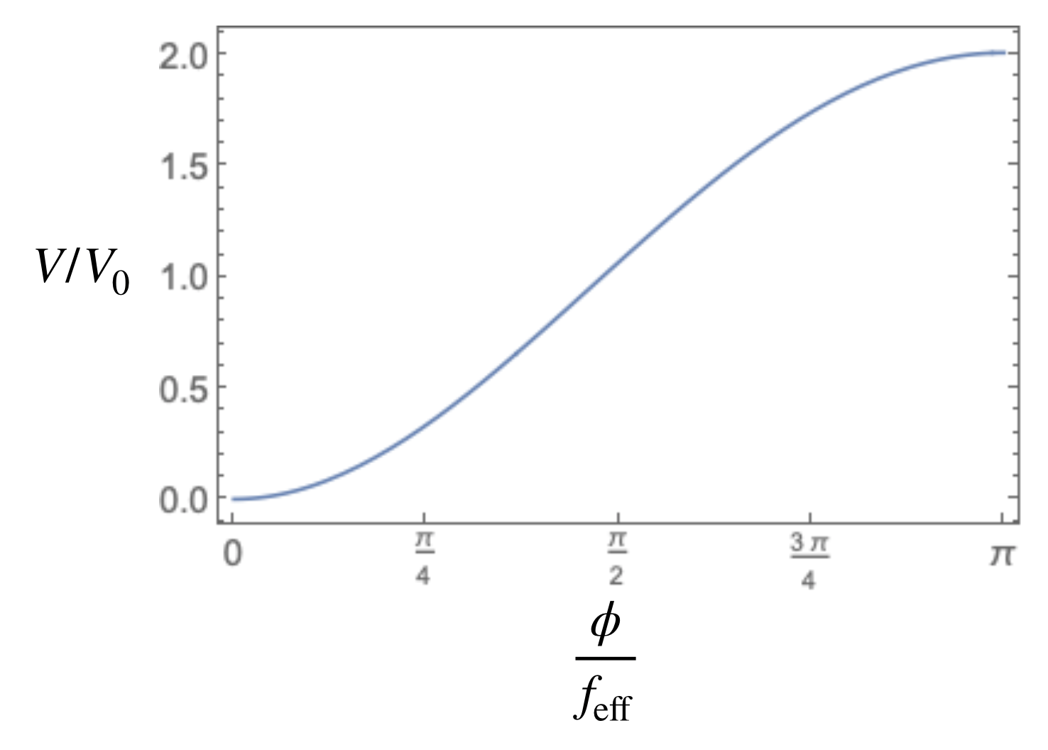
The inflaton potential of minimal gauge inflation model is
| (2) | |||||
where two of the most important model parameters, and , are introduced: is the scale of the potential and is the ‘effective decay constant’. The potential is composed of infinitely many periodic terms. It has a maximum at and we only consider the physical region in . The inflation starts below then roll-down to the true vaccum at . The model may be regarded as a UV completion of the natural inflation models Freese et al. 1990; Adams et al. 1993; Kim et al. 2005. The shape of the potential is depicted in Fig. 1.
II.1 Condition-1
We first request (Condition-1) or . A convenient function is introduced:
| (3) | ||||
| (4) |
The function is plotted in Fig. 2 (upper curve). As the function is monotonically decreasing within the range of our interest, (Condition-1) sets up a upper limit for :
| (5) |
The critical value, , is determined for a given value of . In principle, the parameter is constrained by the inflationary observables. We will be discuss this in Sec. III.

II.2 Condition-2
The potential is convex () for a small field value of then becomes concave () toward the plateau located at the top. The inflection point () locates at . To analyze the second condition, we introduce a convenient function, , which encapsulates the information of the curvature of the potential:
| (6) | ||||
| (7) |
The shape of the is depicted in Fig. 2 (lower curve).
The function is monotonically decreasing and (Condition-2) limits the validity range of and sets the lower bound as
| (8) |
II.3 Condition-1 and Condition-2
In principle, (Condition-1) in Eq. 5 and (Condition-2) in Eq. 8 are independent. However, at least one of the conditions can be satisfied in the whole region of if the lower bound of (Condition-2), , is smaller than the upper bound of (Condition-1), or
| (9) |
This inequality is a generic condition that should be taken as the guiding principle of a model, which has similar features: growing potential having an inflection point in the middle toward the top of the potential. There are many examples of this kind including the Higgs inflation Bezrukov and Shaposhnikov 2008; Bezrukov and Shaposhnikov 2009; Hamada et al. 2014; Hamada et al. 2015; Bezrukov et al. 2015; Bezrukov and Shaposhnikov 2014.
If the above condition is not satisfied, there exists a region of where neither condition is satisfied. Indeed, as one can notice in the figure, in so that one can actually find a set of values for a given value of satisfying the desired condition as one can clearly see in Fig. 2. For instance, with and , thus the dS criterion is satisfied.
In Fig. 3 we depicted the critical lines in the plane of for various values of : . The regions below the lines (colored parts), the critical condition, , is satisfied thus the condition of the refined dS conjecture is fulfilled and belongs to the “Landscape” but in the regions above the lines, the potential may not have a consistent quantum gravitational UV completion or belongs to the “Swampland”.
Until this far, we examine the implications of the refined dS conjecture to generic field space of minimal gauge inflation model. Using the method, we found that the allowed range of depends on . On the other hand, if are known a priori, we can set the theoretically preferred range of the model parameters. Instead, in this paper, we take the observational data as the guideline of a theory and try to set the bound on in the next section.

III Inflationary predictions

The inflationary observables, the power spectrum of the curvature perturbation, , the corresponding spectral index, , the tensor-to-scalar ratio, , of minimal gauge inflation are obtained in Ref. Gong and Park 2018:
| (10) | ||||
| (11) | ||||
| (12) |
where is the number of efolds. From these, we get the model parameters and as
| (13) | |||||
| (14) | |||||
| (15) |
We take the reference values
| (16) |
from the recent data of Cosmic Microwave Background radiation (CMB) from the Planck observatory Akrami et al. 2018; Aghanim et al. 2018; Ade et al. 2016 and also the data taken by the BICEP2/Keck CMB polarization experiments Ade et al. 2018 then we determine the model parameters, and , as well as the allowed window for as
| (17) | ||||
| (18) | ||||
| (19) |
for the requested number of efolds, . Notice that the tensor-to-scalar ratio is within the future probe. The determined values of and would give the compactification radius and the gauge coupling constant:
| (20) |
which look consistent with the quantum gravity and the perturbative gauge theory with .
Finally, having determined the input parameters of the model we now can directly check the dS conjecture. The Fig. 4 is depicted to show the parametric region of which is consistent with the dS conjecture as well as the observational data. The allowed values of and are typically and or smaller. The values are not strictly as requested in the conjecture but still close numerically.
IV Conclusion
The latest swampland conjecture could provide important implications to the low energy effective theory models which may or may not be consistent with the quantum gravity theory. The conjecture suggests two related but independent conditions for any scalar potential of a low energy effective theory of a consistent quantum gravity:
which we call (Condition-1) and (Condition-2), respectively, in this paper. The parameters and are supposed to be universal but unknown positive constants. In this paper, we closely examine a minimal gauge inflation model as a concrete example of potentially realistic inflationary model and apply the dS conjecture to see the consistency with a quantum gravity theory. Interestingly, the potential indeed allows a parametric region in . If we apply the latest cosmological observations from Planck 2018 and also BICEP2+Keck, the allowed region shrinks but still exists as is clearly seen in Fig. 4. Finally, we would emphasize that the method developed in this paper can be applied to any theory with a similarly behaving potential: growing monotonically, having an inflection point on the way to the top.
Acknowledgements.
SC is thankful to Kohei Kamada for valuable comments and Matt Reece for discussion during the CERN-TH institute in summer 2018. This work was supported in part by the National Research Foundation of Korea (NRF) grant funded by the Korean government (MSIP) (No.2016R1A2B2016112) and (NRF-2018R1A4A1025334).References
- Ooguri et al. (2018) H. Ooguri, E. Palti, G. Shiu, and C. Vafa, (2018), arXiv:1810.05506 [hep-th] .
- Obied et al. (2018) G. Obied, H. Ooguri, L. Spodyneiko, and C. Vafa, (2018), arXiv:1806.08362 [hep-th] .
- Tsujikawa (2013) S. Tsujikawa, Class. Quant. Grav. 30, 214003 (2013), arXiv:1304.1961 [gr-qc] .
- Fukuda et al. (2018) H. Fukuda, R. Saito, S. Shirai, and M. Yamazaki, (2018), arXiv:1810.06532 [hep-th] .
- Wang (2018) S.-J. Wang, (2018), arXiv:1810.06445 [hep-th] .
- Das (2018) S. Das, (2018), arXiv:1810.05038 [hep-th] .
- Antoniadis et al. (2018) I. Antoniadis, Y. Chen, and G. K. Leontaris, (2018), arXiv:1810.05060 [hep-th] .
- Ashoorioon (2018) A. Ashoorioon, (2018), arXiv:1810.04001 [hep-th] .
- Motaharfar et al. (2018) M. Motaharfar, V. Kamali, and R. O. Ramos, (2018), arXiv:1810.02816 [astro-ph.CO] .
- Odintsov and Oikonomou (2018) S. D. Odintsov and V. K. Oikonomou, (2018), arXiv:1810.03575 [gr-qc] .
- Dimopoulos (2018) K. Dimopoulos, (2018), arXiv:1810.03438 [gr-qc] .
- Kawasaki and Takhistov (2018) M. Kawasaki and V. Takhistov, (2018), arXiv:1810.02547 [hep-th] .
- Hamaguchi et al. (2018) K. Hamaguchi, M. Ibe, and T. Moroi, (2018), arXiv:1810.02095 [hep-th] .
- Lin et al. (2018) C.-M. Lin, K.-W. Ng, and K. Cheung, (2018), arXiv:1810.01644 [hep-ph] .
- Anguelova et al. (2018) L. Anguelova, E. M. Babalic, and C. I. Lazaroiu, (2018), arXiv:1809.10563 [hep-th] .
- Ellis et al. (2018) J. Ellis, B. Nagaraj, D. V. Nanopoulos, and K. A. Olive, (2018), arXiv:1809.10114 [hep-th] .
- Halverson and Ruehle (2018) J. Halverson and F. Ruehle, (2018), arXiv:1809.08279 [hep-th] .
- Brandenberger et al. (2018) R. Brandenberger, R. R. Cuzinatto, J. Fröhlich, and R. Namba, (2018), arXiv:1809.07409 [gr-qc] .
- Bena et al. (2018) I. Bena, E. Dudas, M. Graña, and S. Lüst, (2018), arXiv:1809.06861 [hep-th] .
- Moritz et al. (2018) J. Moritz, A. Retolaza, and A. Westphal, (2018), arXiv:1809.06618 [hep-th] .
- Visinelli and Vagnozzi (2018) L. Visinelli and S. Vagnozzi, (2018), arXiv:1809.06382 [hep-ph] .
- D’Amico et al. (2018) G. D’Amico, N. Kaloper, and A. Lawrence, (2018), arXiv:1809.05109 [hep-th] .
- Han et al. (2018) C. Han, S. Pi, and M. Sasaki, (2018), arXiv:1809.05507 [hep-ph] .
- Brandenberger (2018) R. H. Brandenberger, (2018), arXiv:1809.04926 [hep-th] .
- Gong and Park (2018) J.-O. Gong and S. C. Park, Chin. Phys. C42, 095102 (2018), arXiv:0801.0333 [hep-ph] .
- Arkani-Hamed et al. (2003) N. Arkani-Hamed, H.-C. Cheng, P. Creminelli, and L. Randall, Phys. Rev. Lett. 90, 221302 (2003), arXiv:hep-th/0301218 [hep-th] .
- Kaplan and Weiner (2004) D. E. Kaplan and N. J. Weiner, JCAP 0402, 005 (2004), arXiv:hep-ph/0302014 [hep-ph] .
- Park (2007) S. C. Park, JCAP 0711, 001 (2007), arXiv:0704.3920 [hep-th] .
- Kubo et al. (2002) M. Kubo, C. S. Lim, and H. Yamashita, Mod. Phys. Lett. A17, 2249 (2002), arXiv:hep-ph/0111327 [hep-ph] .
- Cacciapaglia et al. (2006) G. Cacciapaglia, C. Csaki, and S. C. Park, JHEP 03, 099 (2006), arXiv:hep-ph/0510366 [hep-ph] .
- Freese et al. (1990) K. Freese, J. A. Frieman, and A. V. Olinto, Phys. Rev. Lett. 65, 3233 (1990).
- Adams et al. (1993) F. C. Adams, J. R. Bond, K. Freese, J. A. Frieman, and A. V. Olinto, Phys. Rev. D47, 426 (1993), arXiv:hep-ph/9207245 [hep-ph] .
- Kim et al. (2005) J. E. Kim, H. P. Nilles, and M. Peloso, JCAP 0501, 005 (2005), arXiv:hep-ph/0409138 [hep-ph] .
- Bezrukov and Shaposhnikov (2008) F. L. Bezrukov and M. Shaposhnikov, Phys. Lett. B659, 703 (2008), arXiv:0710.3755 [hep-th] .
- Bezrukov and Shaposhnikov (2009) F. Bezrukov and M. Shaposhnikov, JHEP 07, 089 (2009), arXiv:0904.1537 [hep-ph] .
- Hamada et al. (2014) Y. Hamada, H. Kawai, K.-y. Oda, and S. C. Park, Phys. Rev. Lett. 112, 241301 (2014), arXiv:1403.5043 [hep-ph] .
- Hamada et al. (2015) Y. Hamada, H. Kawai, K.-y. Oda, and S. C. Park, Phys. Rev. D91, 053008 (2015), arXiv:1408.4864 [hep-ph] .
- Bezrukov et al. (2015) F. Bezrukov, J. Rubio, and M. Shaposhnikov, Phys. Rev. D92, 083512 (2015), arXiv:1412.3811 [hep-ph] .
- Bezrukov and Shaposhnikov (2014) F. Bezrukov and M. Shaposhnikov, Phys. Lett. B734, 249 (2014), arXiv:1403.6078 [hep-ph] .
- Akrami et al. (2018) Y. Akrami et al. (Planck), (2018), arXiv:1807.06211 [astro-ph.CO] .
- Aghanim et al. (2018) N. Aghanim et al. (Planck), (2018), arXiv:1807.06209 [astro-ph.CO] .
- Ade et al. (2016) P. A. R. Ade et al. (Planck), Astron. Astrophys. 594, A13 (2016), arXiv:1502.01589 [astro-ph.CO] .
- Ade et al. (2018) P. A. R. Ade et al. (BICEP2, Keck Array), (2018), arXiv:1810.05216 [astro-ph.CO] .