Lightweight Structure Design Under Force Location UncertaintyJournal: TOGVolume: 94393DOI: 0000001.0000001_2CCS: Computing methodologies Shape analysisCCS: Computing methodologies Mesh modelsCCS: Applied computing Computer-aided designJournal: TOGVolume: 3641587DOI: http://dx.doi.org/10.1145/3072959.3073626

Abstract.
We introduce a lightweight structure optimization approach for problems in which there is uncertainty in the force locations. Such uncertainty may arise due to force contact locations that change during use or are simply unknown a priori. Given an input 3D model, regions on its boundary where arbitrary normal forces may make contact, and a total force-magnitude budget, our algorithm generates a minimum weight 3D structure that withstands any force configuration capped by the budget. Our approach works by repeatedly finding the most critical force configuration and altering the internal structure accordingly. A key issue, however, is that the critical force configuration changes as the structure evolves, resulting in a significant computational challenge. To address this, we propose an efficient critical instant analysis approach. Combined with a reduced order formulation, our method provides a practical solution to the structural optimization problem. We demonstrate our method on a variety of models and validate it with mechanical tests.
Keywords:
structural analysis, structural optimization, digital fabrication1. Introduction
With the emergence of additive fabrication technologies, structural optimization and lightweighting methods have become increasingly ubiquitous in shape design [Stava et al. 2012; Wang et al. 2013; Lu et al. 2014; Christiansen et al. 2015]. In many such methods, a common approach is to model the external forces as known and fixed quantities. In many real world applications, however, the external forces’ contact locations and magnitudes may exhibit significant variations during the use of the object. In such cases, existing techniques are either not directly applicable, or require the designer to make overly conservative simplifications to account for the uncertainty in the force configurations [Choi and Park 2002].
We propose a new method for designing minimum weight objects when there exists uncertainty in the external force locations. Such uncertainties may arise in various contexts such as (i) multiple force configuration problems where the object experiences a large set of known force configurations such as those arising in machinery, (ii) unknown force configuration problems where the location of the contact points may change nondeterministically such as consumer products that are handled in a multitude of ways, or (iii) moving contact problems where a contact force travels on the boundary of an object; such as automated fiber placement manufacturing or cam-follower mechanisms.
Our approach takes as input (1) a 3D shape represented by its boundary surface mesh, (2) a user-specified contact region; a subset of the boundary where external forces may make contact, and (3) a force-budget; a maximum cap on the total summed magnitude of the external forces at any given time instance, and produces a minimum weight 3D structure that withstands any force configuration capped by the budget (Figure 1).
For structural optimization with force location uncertainties, a seemingly reasonable approach would be to compute an optimal structure for every possible force configuration and select the best structure at the end. However, this strategy fails to guarantee that the final structure (or any other optimum structure computed along the way) is safe under any force configuration other than the one it was computed for [Banichuk 2013]. Therefore, at a minimum, finding the best structure requires validating each optimum structure against all possible force configurations. Unfortunately, even this strategy does not guarantee that a solution exists within the set of computed optima.
Our approach overcomes these challenges using a critical instant analysis which efficiently determines the most critical force contact location responsible for creating the highest stress within the current shape hypothesis. This capability enables each step of the shape optimization to efficiently determine the maximum possible stress that can be generated under the force budget and accordingly design the material distribution against failure. Our approach preserves the outer shape through an ingrown boundary shell while optimization removes material from the inside. We do not permit structural alterations to the exterior of the object for strengthening. Hence, our approach is clearly not useful in cases where material failure occurs even in the fully solid version of the object.
Our main contributions are:
- •
a novel formulation for structural optimization problems under force location uncertainty,
- •
a method we call critical instant analysis that identifies the critical load instant quickly,
- •
a practical reduced order lightweighting method using the above two ideas.
2. Related Work
Our review focuses on studies that highlight fabrication oriented design, lightweight structure synthesis, and structural analysis, with an emphasis on approaches involving additive fabrication.
Fabrication oriented design
A large body of work has investigated automatic techniques for 3D shape design and additive fabrication subject to a variety of functional requirements. Recent examples include designing for prescribed deformation behaviors [Bickel et al. 2010; Skouras et al. 2013; Schumacher et al. 2015; Panetta et al. 2015], balancing models [Prévost et al. 2013], spinnable objects [Bächer et al. 2014] and broader methods that can handle multiple requirements [Chen et al. 2013; Musialski et al. 2015; Christiansen et al. 2015]. Our problem falls under the general category of weight-optimal structure design subject to external forces [Bendsøe 1989; Wang et al. 2013; Lu et al. 2014; Christiansen et al. 2015]. However, our approach addresses a more general class of problems in which the precise force locations cannot be prescribed apriori, or the structure experiences forces that can contact its surface at a multitude of locations.
Lightweight structure synthesis
Cellular structure [Medeiros E Sá et al. 2015], honeycomb-like structure [Lu et al. 2014], truss element based skin-frame structure [Wang et al. 2013], beam element based tree-like structure [Zhang et al. 2015] generation methods and topology optimization methods [Christiansen et al. 2015; Bendsøe and Sigmund 2003] are among the recent lightweight internal structure synthesis techniques that consider durability as one of the primary constraints. However, these methods assume a prescribed static force configuration for structural design. Although driven by similar motivations, our work addresses a more general problem of structural design under force location uncertainty. On the other hand, our formulation is also complementary in that it may facilitate the extension of these previous methods to problems involving force uncertainties.
Langlois et. al. [Langlois et al. 2016] performs structural optimization by predicting the failure modes of objects in real world use. Their stochastic finite element model uses contact force samples generated by rigid body simulations to predict failure probabilities. They perform weight minimization while limiting the failure probability below a prescribed threshold. While their method is applicable to scenarios where loading is stochastic in nature (such as dropping and collisions), it is not streamlined for deterministic scenarios where the set of possible force configurations are known and no failure is tolerated for any of them. However, their method is extremely well-suited to automatically generating our contact regions, thereby allowing stochastic scenarios they consider to be addressed using structural guarantees our approach enables.
Model reduction has been used for material [Xu et al. 2015] design, with a primary emphasis on controlling deformation behavior. Our approach is similar to traditional topology optimization methods [Bendsøe and Sigmund 2003; Lee et al. 2012] in that we optimize the material distribution using a fixed volumetric mesh as the parameterization. However, structural optimization under force location uncertainties introduces computational challenges that make a full dimensional analysis using the original shape parameterization to be prohibitively expensive. We are thus inspired by the above reduction method for shape synthesis, and use this in our implementation in conjunction with our new critical instant analysis.
Musialski et al. [Musialski et al. 2015] introduce the idea of offset surfaces for hollowing out a solid object. This method serves as another shape parameterization for functional optimization. In our work, we use this method to form a fixed, ingrown boundary shell, and use the remaining internal volume for shape optimization.
Structural analysis
In structural optimization, stress and deformation analysis using Finite Element Analysis (FEA) often introduce expensive computational bottlenecks. Simple elemental structures such as trusses [Smith et al. 2002; Rosen 2007; Wang et al. 2013] and beams [Zhang et al. 2015] have been used to alleviate this issue. For cases where the structure cannot be represented by these simple elements, Umetani and Schmidt [Umetani and Schmidt 2013] simplify the problem into 2D cross-sections and extend the Euler-Bernoulli model into free-from 3D objects to facilitate analysis.
Zhou et al. [Zhou et al. 2013] extend modal analysis used in dynamic systems (such as vibrations) to static problems to identify the potential regions of a structure that may fail under arbitrary force configurations. Our critical instant analysis builds upon this approach; we use modal analysis to determine the weak regions in a similar manner. It allows our method to determine possible failure points based purely on geometry, i.e. independent of the loading. We incorporate the weak region analysis into our structural optimization to focus on only a small region in the object to monitor the stress, thereby helping the convergence.
In bridge (traffic load) and building (wind load) design, an equivalent uniformly distributed static load can be used to perform simple approximate analysis to account for force location uncertainty [Choi and Park 2002]. However, this approach is limited to simple geometries, making it unsuitable for our purposes.
3. Problem Formulation
Our design problem aims to find an optimal material distribution inside the boundary surface mesh parametrized by the discretized volumetric mesh. Similar to topology optimization [Bendsøe and Sigmund 2003], material design [Skouras et al. 2013; Xu et al. 2015] and microstructure design [Schumacher et al. 2015] approaches, each element in the discretized domain is associated with a design variable representing whether element is full () or void (). To overcome the computational barriers introduced by binary variables, we adopt the common approach of allowing and penalize the intermediate values during optimization [Bendsøe 1989]. We assume linear isotropic materials and small deformations. The elemental stiffness matrix can be related to and the stiffness matrix for base material as
| (1) |
Here, is a penalization factor and is the stiffness matrix assigned to the void regions to avoid singularities in FEA. We use and . In (1), is constant for each element and is computed as
| (2) |
where is volume of the element, is the strain-displacement matrix that depends only on the element’s rest shape and is the elasticity tensor constructed using the Young’s modulus and Poisson’s ratio of the base material. Given a volumetric mesh with elements, one can assemble into vector and construct the global stiffness matrix in order to determine the displacements from , where is the nodal force vector. Then, the stress-displacement relationship can be written as
| (3) |
where captures the unique six elements of the elemental stress tensor and is the assembly of matrices. Block-diagonal matrix is constructed with elemental elasticity tensors on the diagonal. For each element, can be computed analogous to in (1). While applicable to different element types, we use linear tetrahedral elements making , , and for a volume mesh having nodes.
The approach formulated in (1)-(3) is useful because it preserves the same discretization through out the optimization. Additionally, it is amenable to model reduction presented in Section 5 for more efficient iterations (at the expense of reduced degrees freedom).
Force Model

External forces are allowed to make contact within a user-specified union of contact regions . To avoid stress singularities (i.e. unbounded stresses under a point force), we distribute the force to a small circular area (with radius ) around the contact point. Then, we construct the force vector by computing the nodal forces as
| (4) |
where is the force vector at node when a force with magnitude is applied to node . The area is the portion of covered by triangles adjacent to node and is the surface normal at node (Figure 2). Our approach approximates by intersecting the boundary mesh with a sphere of radius centered at node . Congruent with our earlier problem description of normal contact forces only, (4) assumes the force is applied compressively along the surface normal direction. This formulation thus neglects friction and excludes forces that pull on the surface. Note, however, that most real-world contact scenarios such as handling a part or the contacts within an assembly can be modeled with compressive normal forces developing between interacting bodies.
To anchor the object in space, we require that the mesh is fixed at three or more non-collinear boundary nodes. Boundary constraints remain unchanged during optimization.

In this work, we use the von Mises failure criterion. For linear elastic structures, the stress is a linear function of dispacement and the displacement at any given point is a linear function of the force vector. Similarly, the force vector is a linear combination of point normal forces in the contact region. Thus, the stress at a point within the structure can be determined by a superposition of each point force’s contribution [Hibbeler and Kiang 2015], thereby making the von Mises stress convex in the applied force. For the force budget , the space of allowable forces is defined by and , i.e. a simplex with vertices of the form for j’th coordinate and zero for the rest and the coordinate origin. By Rockafellar’s Theorem 32.2 [Rockafellar 2015], supremum of a convex function on a convex set is attained at one of the points in the set enclosed by the convex hull . Therefore, von Mises stress at a point will be maximized by spending the entire force budget at a specific point. The same principal holds for the maximum of the von Mises stress over the whole object as a maximum of a set of convex functions is convex. As a result, at the heart of our approach is the search for this most critical contact point given a shape hypothesis (Section 4.2)
Optimization problem
We tackle the following stress-constrained mass minimization problem
| (5) | ||||||
Here, and represent the nodal force and displacement vectors when the external force is applied to surface node . The object fails if the maximum stress ever exceeds the yields strength . Hence, we define the critical stress as
| (6) |
where is the von Mises stress computed for element .
4. Algorithm
For force instant , all elemental von Mises stresses (hence the maximum) within the object can be computed using (3) with a single linear solve. However, finding the maximum across all possible instants require as many FEA solves as the number of instants. This number can be large, especially for structures where consist of many nodes. In such cases, computing the critical stress can be costly, making shape optimization prohibitively expensive. We next describe our approach to addressing this problem.
4.1. Overview
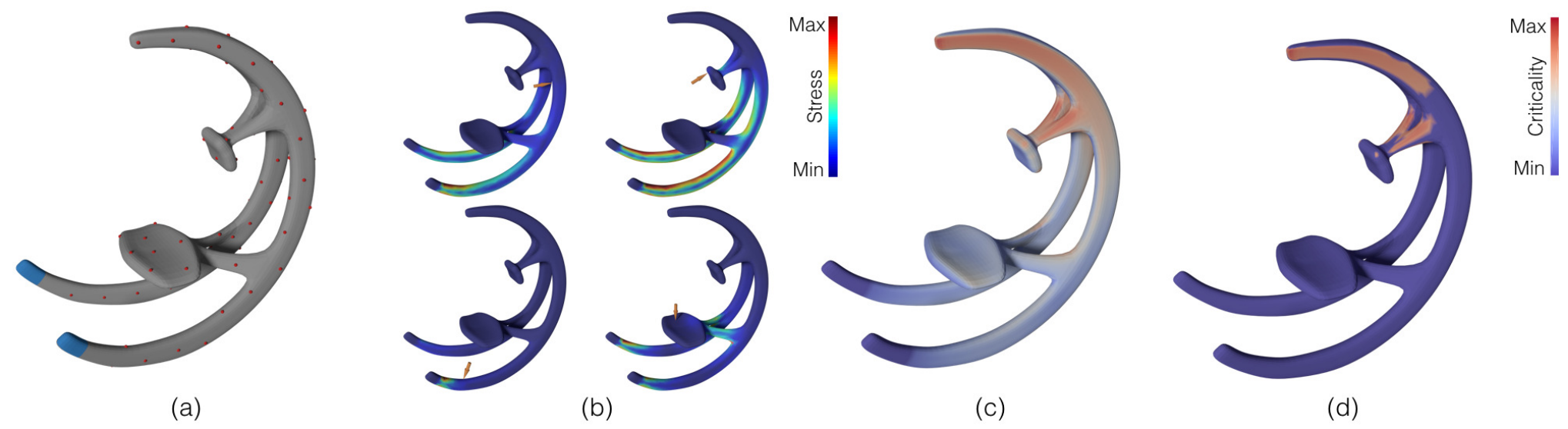
Figure 3 illustrates our approach. From an input 3D shape and prescribed contact regions (Figure 3(a)), we optimize the material distribution. At each step governed by the current material distribution, we compute the critical stress by efficiently finding the most critical force instant. We call this process critical instant analysis. In this analysis, we reduce the search space by computing a set of force regions (FR) over the contact region and weak regions (WR) within the entire structure . FRs are a subspace of the surface that are likely to contain the critical force instant. Likewise, WRs are the regions where the maximum stress is likely to occur. We efficiently find the critical force instant within FRs using a reduced number of FEA evaluations dictated by the number of vertices within FRs. Then, optimization updates the material distribution to minimize mass (Figure 3(b-c)). At the end, a minimum weight structure satisfying the imposed constraints is obtained (Figure 3(d)). Algorithm 1 summarizes our approach. Note that the material distribution is updated only once at each optimization step based on the computed gradients.
4.2. Critical Instant Analysis
Critical instant analysis finds the most critical force instant and the corresponding stress with an order of magnitude fewer FEA evaluations compared to a brute-force approach.

Force Regions
For a structure represented by material distribution , certain force configurations will cause the largest stresses in the body. We compute these critical force locations as our force regions and restrict the search space for in (6) to a smaller space .
Figure 4 illustrates our approach to compute FRs. We start by estimating a criticality map on , which captures the severity of the force instants. The higher stress a force instant creates, the more critical it is deemed. Thus, the criticality of a force instant is simply the maximum stress it creates in the object.
To efficiently acquire the entire criticality map, we perform FEAs only for a small number of force instants and estimate the stress distributions for remaining force instants by learning a mapping between the nodal forces and the resulting stress distributions. We sample the force instants across by performing k-means clustering using the farthest-first traversal initialization and selecting the center points of the resulting clusters as our sample instants. We use approximate geodesic distances [Crane et al. 2013] as the distance metric in clustering.
Suppose we have training samples and the boundary mesh consists of nodes. In its original form, the sample force instant is represented as a sparse vector of size and the corresponding von Mises stress forms a vector of size . With a small number of training samples ( and ), it is not possible to represent the relationship between two high dimensional data using a simple mapping function. Moreover, in its sparse form, is devoid of any spatial information relevant to the corresponding force instant. Hence, in this representation, two spatially proximate force instants that likely create similar stress distributions can be as distinct as two spatially distant force instants. To reduce the dimensionality of the force space and establish proximity, we transform and project the sparse force vectors using the surface Laplacian. We stack the magnitudes of forces on boundary surface nodes (i.e. in (4)) into row vectors of length . We assemble the mean centered into a matrix so that each row is where is the average of . We then compute the Laplacian basis functions as the eigenvectors of the surface graph Laplacian . We assemble the first eigenvectors to form our lower dimensional basis matrix . The lower dimensional representation of the force instants can then be written as
| (7) |
where becomes an matrix.
Similarly, we use principal component analysis (PCA) to project the stress data onto a lower dimensional space. We assemble the mean centered stress vectors into an matrix . A PCA on yields principal vectors of size . Then, each stress vector can be approximated by PCA weights through a linear combinations of the principal vectors
| (8) |
where is matrix storing the PCA weights for each sample in its rows and is the assembly of principal vectors.
Lower dimensionality in and allows us to learn a simple mapping between the two spaces with a reasonable computational cost. We have found that quadratic regression with L2 regularization performs sufficiently well for capturing the relationship between the PCA weights of the stress vectors and the reduced dimensional force vectors such that . Here, is matrix including the quadratic terms for . In matrix form, the coefficient matrix can be computed as
| (9) |
where is a small number controlling the importance of the regularization term. Using this map, we estimate the criticality of a new force instant by computing the stress distribution it creates through the quadratic map, and extracting its maximum. Note that the estimated stress vectors are only an approximation of the actual values, thus cannot be used directly for . However, they provide strong guidance in estimating the location of the most critical force instant. We thus use the synthesized criticality map to determine the force regions (Figure 4(d)). The connected components of high criticality areas in comprise our force regions.
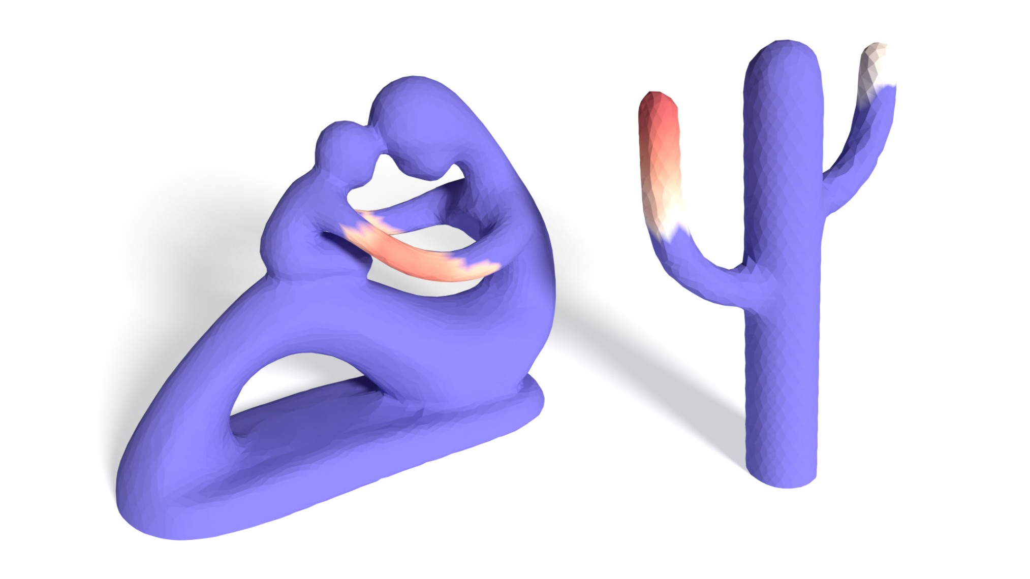
The accuracy of the criticality map depends on the number of training samples . While a large number of samples increases accuracy, the computational cost also increases proportionally. Figure 5 illustrates the criticality maps obtained with different number of training samples. We observed that using of the nodes in for training produces an acceptable approximation of the criticality map such that in all of our examples, after the criticality values are estimated, top of the nodes with the largest criticality values always contain the ground truth critical instant. Figure 6 illustrates the force regions we obtained for two different models.
Weak Regions
For a structure with material distribution , we need to find the maximum stress produced by each force instant to determine in (6) and solve (5). However, failure often occurs at certain regions of the object leaving the remainder safe at all times. WRs help us constrain the regions of the structure where we seek the maximum stress .
In our algorithm, we use an approach similar to [Zhou et al. 2013] to determine the possible failure locations as our weak regions. We determine WRs using modal analysis that involves solving the generalized eigenvalue problem
| (10) |
where is ’th eigenmode, is the corresponding eigenvalue and is the mass matrix for the tetrahedral mesh. Note that WRs are structure dependent, hence need to be updated at each step of the optimization. To reduce computational cost, we use a lumped mass matrix and distribute each element’s mass to its nodes equally, thus creating a sparse diagonal matrix .
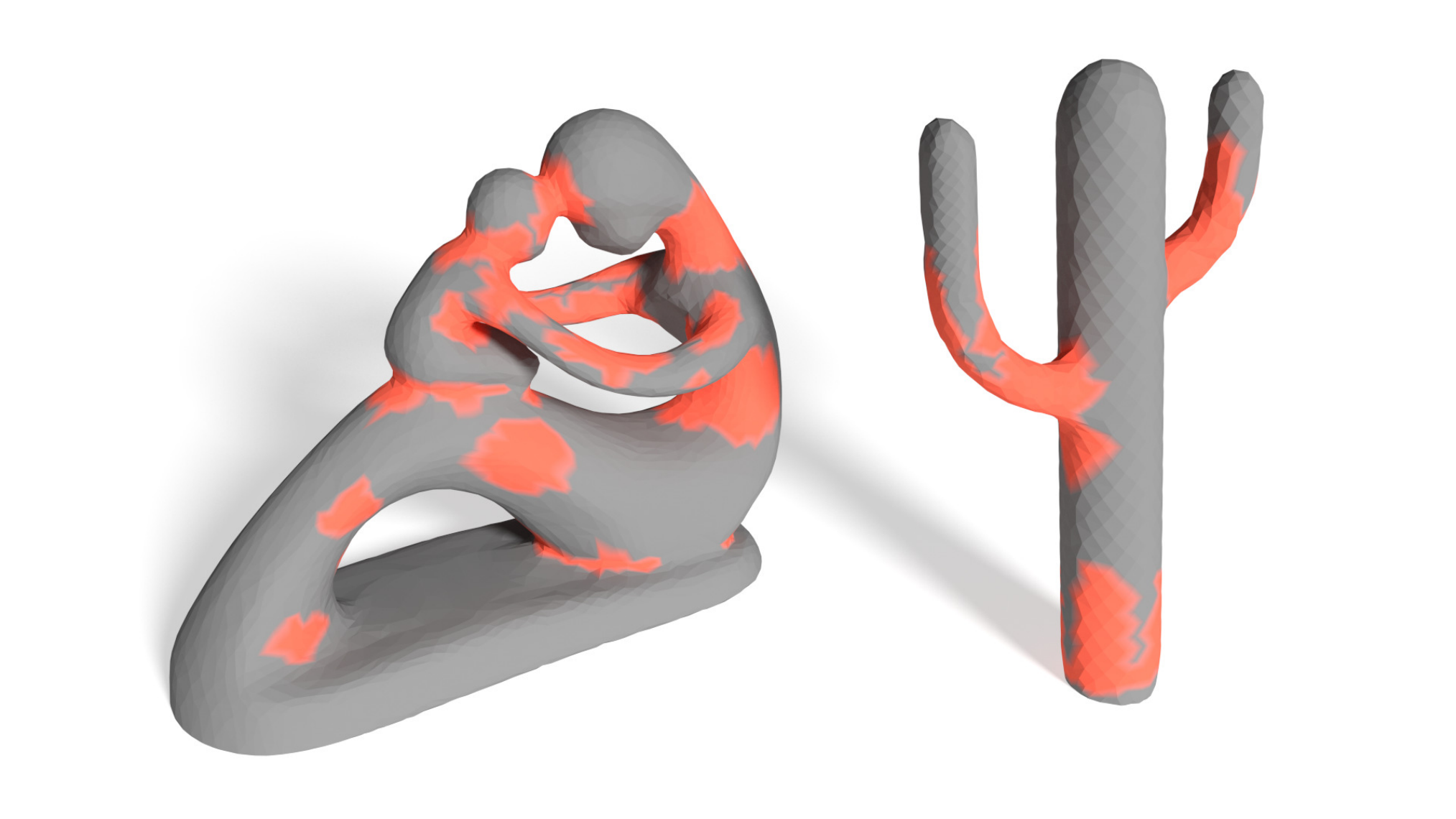
WRs can be extracted by computing the low frequency eigenmodes in (10) and identifying the nodes that experience large stresses under these deformations. In our examples, we use the first vibration modes and of the most stressed nodes to form our WRs. Different from [Zhou et al. 2013], we combine all unique nodes obtained from modal analysis to construct the WRs. Figure 7 shows the WRs we obtained for two fully solid models (). Note that WRs are found around possible stress concentration points such as thin parts and crease edges.
Critical Instant
We solve (6) for in a much smaller domain defined by the FRs and WRs . In particular, only the force instants captures with FRs are used, and maximum stresses are only sought in WRs.
We use a simple greedy hierarchical search to find the force instant creating the largest stress in the structure. For each FR island, we partition it into four segments and perform FEA by applying the force to their central nodes. We then further select and partition the segment that produces the highest stress within WRs, and repeat this process until converging to a single node. After repeating this process for all FR islands, we choose the maximum stress across all FR islands as for that particular optimization step. The stiffness matrix and need to be computed only once during these evaluations as the structure remains unchanged. We thus factorize once for each optimization step, and determine displacements and stresses using efficient forward and backward substitutions.
4.3. Stress Singularity
Stress constrained mass minimization problems are prone to singularity issues [Sved and Ginos 1968; Kirsch 1990; Lee et al. 2012]. For instance, in (5), the global optimum is obtained when , making all elements void. To mitigate this problem, we establish a layer of fully solid boundary shell that is excluded from optimization. This approach overcomes the singularity problem by coercing the optimization to employ material in the remaining inner volume as a way relieve the high stresses generated on the boundary shell. Enforcing a boundary shell also preserves the original outer surface.
All elements that contribute one or more vertices to the outer boundary could serve as the boundary elements. For an arbitrary volumetric mesh, however, forming a solid shell using only these elements may introduce stress concentrations (Figure 8(a)). To create a smooth and uniform thickness shell, we first generate an inner offset surface using the method presented in [Musialski et al. 2015]. Then, we tetrahedralize the entire domain, which results in a smooth shell layer sandwiched by and (Figure 8(b-c)). We use a uniform shell thickness prescribed by the user, which can be adjusted based on a 3D printer’s minimum print thickness. Although we do not optimize the shell thickness, we discuss its effects in Section 6.
5. Model Reduction
The optimization problem (5) is typically very high-dimensional as the number of design variables is equal to the number elements in the volumetric mesh . This, in turn, has a significant impact on the computational performance. To accelerate optimization, we compute a set of material modes [Xu et al. 2015], which helps control the material distribution using only a small number of variables. Material modes can be computed as the eigenvectors of the element-based graph Laplacian defined on by solving the generalized eigenvalue problem
| (11) |
where are non-negative eigenvalues, are corresponding eigenvectors and is a diagonal matrix composed of s. Eigenvectors are orthogonal and smooth scalar functions that spectrally decompose the material distribution [Zhou et al. 2005; Zhang et al. 2010]. The first mode represents the homogeneous material distribution and while the level of detail control increases with higher frequencies (Figure 9). We assemble the first eigenvectors to form the reduced order basis so that the material distribution can be written as
| (12) |
where is the design vector for the reduced order problem. This formulation allows us to trivially enforce fully solid material on the boundary shell elements by by setting the corresponding rows in the reduced basis matrix to be . This way the entries in can take on any value during the optimization without violating the geometrical constraints.

Logistic Function
In our reduced order formulation, we use a logistic function to penalize the intermediate values of by modifying (12) as
| (13a) | ||||
| (13b) | ||||
Here, and determine the steepness and inflection point of the logistic function. Note that should be adjusted to satisfy to ensure that the elements on the boundary shell are solid. While increasing intensifies binarization by pushing the intermediate densities toward and , it also hampers convergence. We use for all of our examples.
In addition to binarizing the intermediate densities, the use of logistic function in (13a) guarantees for . This allows us to remove a large number of constraints from our reduced order optimization problem.

5.1. Reduced Order Problem
Applying (13) to our optimization formulation (5), the reduced order optimization problem can be stated as
| (14) | ||||||
where
| (15) |
for .
A benefit of the reduced order formulation is that the number of new design variables can be markedly small compared to the number of original variables in (5). This number is independent of the input mesh and needs to be prescribed by the user. Because the structural optimization algorithm involves a large number of costly FEA evaluations per iteration, we found to provide a favorable tradeoff between speed and expressiveness. Hence, we use material modes in all of our examples, unless otherwise stated. The optimization starts with a fully solid model (). Our approach is predicated on the assumption that this starting solution is feasible, hence amenable to lightweighting through optimization.
At the end of the optimization, the resulting material distribution may still contain elements with intermediate densities. In such cases, we threshold the gray scale material distribution to obtain a fully binarized solution. In our examples, we use as the threshold; elements with lower densities are set to void. Nonetheless, there exists more sophisticated thresholding methods [Hsu and Hsu 2005]. Another positive byproduct of the reduced order approach is that the resulting material distribution after binarization typically does not suffer from a checkerboard effect, as the reduction leads to smooth material modes in , especially for . This, in turn, helps alleviate exhaustive post-processing.
Note that the material modes are precomputed as they depend only on . Because only the first modes are used in the reduced order formulation, they can be computed efficiently using iterative methods. We use ARPACK for this purpose [Lehoucq et al. 1998]. In order to solve (14), we use sequential quadratic programming [Nocedal and Wright 2006]. Our code solves linear systems using the Eigen library’s SimplicialLDLT sparse solver [Guennebaud et al. 2010].
Our hierarchical search method and density based shape representation allow us to compute gradients analytically. We compute gradients of the critical stress with respect to the design variables using the adjoint method [Paris et al. 2010]. We use p-norm approximations () for the max functions. Details are given in Appendix A.

6. Results and Discussion
6.1. Criticality Analysis
Figure 10 illustrates the results of our critical instant analysis on a collection of fully solid models. In all cases presented in this paper, our approach involving criticality map estimation followed by a hierarchical search is able to determine the true critical force instant (yellow arrows). We verified this match using an expensive brute force search method. As shown in Figure 10, our estimated criticality map captures the true critical instant quite well in that it finds the most critical force to be at the point with the highest estimated criticality (dark red). Nonetheless, our analysis can tolerate inaccuracies in the estimated criticality map. Figure 11(a) shows such a case. Although the criticality map estimates the most critical point to be on the arm closer to the baby (dark red), our algorithm subsequently finds the true critical instant in that vicinity by searching an expanded area forming the force region.


Figure 11 illustrates the critical instants for two different material distributions. Because we construct the criticality map for each step of the optimization, the force regions are updated and the change in the critical instant is captured well. In all of our examples, the critical force instant is always contained in the identified force regions.
Comparison
Figure 12 compares our critical instant analysis with the worst-case structural analysis of Zhou et. al. [Zhou et al. 2013]. The worst-case structural analysis method is designed to predict the critical force configurations that develop during handling an object. Thus, it may have a tendency to overpredict the weakness, resulting in overengineered solutions if used for structural optimization. In our method, because we delineate the contact regions and the displacement constraints to reflect the knowledge of actual use, our approach captures the critical forces that are more likely to be encountered during a product’s nominal use. For instance, the region encircled in Figure 12 for our analysis shows the high stress region worst-case analysis fails to capture. The boundary conditions and the contact regions used in our analysis are shown in Figure 13.
6.2. Structural Optimization
Figure 13 illustrates the results of our method on various 3D models. The displacement-constrained regions are shown in blue. The contact regions are shown in green. Our reduced order optimization detects the parts of the objects where high stresses may develop and distributes material accordingly. For objects with small weak regions such as the fertility and penguin models, our optimization allows us to preserve the same structural strength that their fully solid versions possess, while shedding a large portion of the mass. Similarly, our algorithm performs well for models with thin elements such as the chair by utilizing mass around the stress carrying regions of the object. Notice the arms supporting the seat in the rocking chair and the back support in the chair model.
In these examples, we achieved to mass reduction. Table 1 summarizes the weight reduction together with various other metrics relevant to these models.

Comparison
In Figure 14, we compare our approach with the build-to-last method [Lu et al. 2014]. We impose a force budget of applied anywhere on the surface of the shark. Our optimum result weighs less than the build-to-last structure that takes a prescribed force location as input11 1 In [Lu et al. 2014], we could not identify the force magnitude being used.. Unlike build-to-last, our algorithm hollows the fins and the nose where high stresses cannot be generated in any force configuration. Also, our method generates a three-pronged rib structure at the base, possibly to accommodate the forces that can be applied laterally in all arbitrary directions.

Number of Material Modes
Figure 15 illustrates the effect of the number of material modes. We optimized the bracket using , and modes for the same force budget and boundary conditions. As shown, higher material modes allow for a finer local shape control. Hence, a larger mass reduction is obtained with increasing number of material modes (see Table 1). Although larger number of modes allow our algorithm to remove more material through local control, computational cost also increases. In Table 1, per iteration computation times are given for the bracket model using different number of material modes. As the number of modes increases, computational cost increases significantly, while only a minor improvement in further mass reduction is achieved.
Convergence
Figure 16 shows the convergence profiles for the bracket model. While convergence is achieved after a similar number of iterations, the smaller number of material modes tend to leave more intermediate density elements in the optimized distribution, resulting in a larger mass when binarized.
One might worry that in a symmetrical object, the critical point could jump from side to side, with every incremental improvement to one side causing a symmetric worsening of the other side, and convergence never being reached. We attempted to trigger this potential failure by creating a test case with a carefully-constructed perfectly symmetric boundary and tetrehedral mesh (Figure 17). Our algorithm nonetheless converged in steps. We conjecture that the homogenous (first) material mode tends to absorb enough of the change to avoid oscillation; though it could also be that low-level numerical asymmetries, e.g. ordering effects in linear algebra routines, account for the convergence.


Boundary shell thickness
There is a trade-off between the shell thickness and the flexibility of our algorithm in generating an internal structure. As the boundary shell gets thicker, its contribution to the structure’s strength becomes more prominent, thereby shrinking the design space for our algorithm. On the other hand, too thin boundary shells can lead to large local compressive stresses that renders optimization infeasible. In such cases, our method fails to converge to a varied solid versus void material distribution (Figure 18(a)). The main reason is that high local compressive stresses encourages the optimization to perform local thickening around the force application points. However, low frequency modes can alter the material distribution only in large chunks. Therefore, fine-level local modifications cannot be achieved unless a large number of material modes are used. Figure 18 illustrates the effect of the shell thickness on the resulting material distribution. With a proper choice of the thickness (Figure 18(b)), our method is able to reduce mass by compared to fully solid model, while the reduction was only and for (a) and (c), respectively.
6.3. Validation and Performance
Fabrication
We 3D printed our optimum results on an OBJET Connex printer using inkjet printing technology. We use VeroWhitePlus material with a yield strength of , a Young’s modulus of , and a Poisson’s ratio of [PolyJet 2017].
When soluble support material is used, the boundary shell can be pierced by small holes to empty the internal support material. We observed that our reduced order method has a tendency to create only a small number of inner void regions (especially for a small number of material modes) and thus the support material can be removed with minimal alterations. To avoid trapping support material, resulting models can be printed in several pieces and glued together after cleaning.
Physical Tests
We performed compression tests on our optimized cactus model to physically evaluate the strength of the 3D printed models, as shown in Figure 19. We used an INSTRON universal testing machine and ran compression tests on the optimized cactus model. For comparison, we chose an identically weighing uniform thickness cactus. We performed the same compression test on the long arm and measured the failure load. For our optimized model, we measured the failure force to be . The uniform thickness model snapped at less force of .

For our optimized model, we measured the failure force of for the short arm, and for the trunk. The test results agree well with our critical instant analysis in that the tip of the long arm turns out to be physically the most critical force point in the optimum model and there is no need to add material to either the short arm or the trunk. Figure 20 illustrates the stress distribution when a force is applied to the same three points as the physical tests. It can be observed that the short arm and the trunk are quite safe, while very high stresses are present on the long arm.
| Model | Elements | # of FEA | Analysis Time [s] | Iteration | Time[s] | Volume [cm3] | |||
|---|---|---|---|---|---|---|---|---|---|
| Brute Force | Our Method | Brute Force | Our Method | Initial | Optimized | ||||
| Cactus | 25229 | 1658 | 216 | 17.69 | 4.35 | 49 | 39.61 | 68.990 | 18.800 |
| Slingshot | 54290 | 2192 | 148 | 89.02 | 10.66 | 124 | 72.52 | 17.822 | 9.451 |
| Fertility | 57006 | 3914 | 248 | 131.85 | 20.68 | 122 | 83.33 | 54.023 | 16.350 |
| Test (Small Force) | 58555 | 822 | 69 | 26.53 | 7.52 | 180 | 59.15 | 4.443 | 1.216 |
| Test (Large Force) | 58555 | 822 | 69 | 26.53 | 7.52 | 223 | 59.15 | 4.443 | 1.300 |
| Chair | 58848 | 663 | 52 | 27.96 | 13.28 | 104 | 75.32 | 17.076 | 6.192 |
| Penguin | 68615 | 3035 | 304 | 149.80 | 45.13 | 31 | 132.06 | 91.643 | 10.211 |
| Shark | 70397 | 4282 | 273 | 178.93 | 18.10 | 72 | 115.07 | 66.454 | 14.997 |
| Rocking Chair | 78025 | 1531 | 103 | 85.48 | 11.17 | 160 | 154.32 | 13.015 | 6.709 |
| Bracket (k = 15) | 111498 | 408 | 55 | 70.85 | 48.87 | 39 | 301.01 | 462.520 | 194.434 |
| Bracket (k = 50) | 111498 | 408 | 55 | 70.85 | 48.87 | 38 | 382.49 | 462.520 | 167.552 |
| Bracket (k = 100) | 111498 | 408 | 55 | 70.85 | 48.87 | 37 | 487.44 | 462.520 | 163.581 |
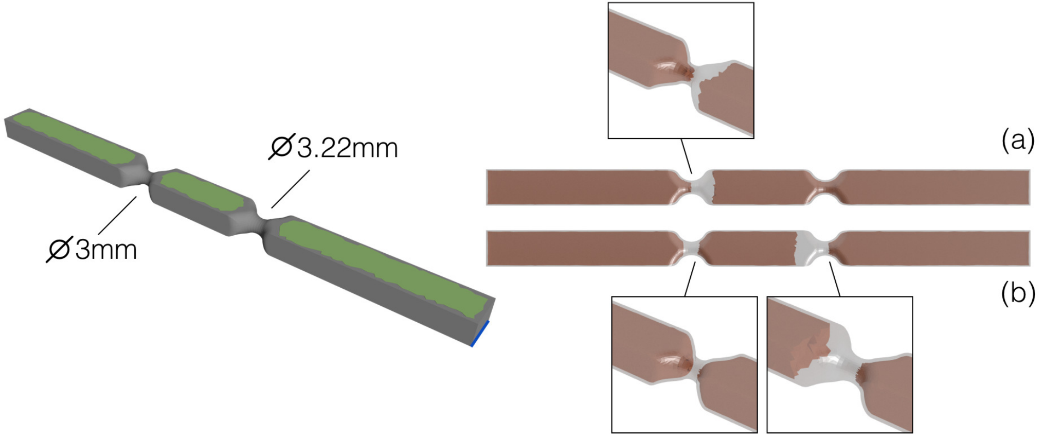
Figure 21 illustrates a test model we designed to observe the effect of the force budget. The model has two thin regions with slightly different dimensions. We set the contact region to be the entire top surface while fixing it only at the bottom right and left edges to simulate a simply supported beam. We then optimized the structure for two different force budgets of and . For the smaller force budget, the optimization focuses material around the thinnest part only. However, for the larger force budget, material is distributed around both of the failure prone regions. Notice that only a portion of the thinnest neck is filled for the small force budget while it is entirely filled for the larger force budget. To validate the optimization results of the test model, we performed a set of three-point bend tests. For benchmarking, we also tested a completely empty shell model (full-void). Figure 22 shows the experimental setup together with the force plots we obtained. The test model optimized for the larger force budget performs best while the empty model breaks at the smallest force magnitude. Our structural optimization method strengthens the model up to while increasing its mass by only . The discrepancies between the input force budget and the measured failure forces can be due to the FEA modeling of the problem as well as the possible anisotropic behavior of the 3D printed material [Ulu et al. 2015].


Performance
Table 1 shows the performance of our algorithm. We tested our method on a 3.2GHz Intel Core i5 computer with 8GB of memory. We selected various 3D models and optimized under different force configurations. Although the major computational cost comes from the critical instant analysis, we achieve acceleration on average over a brute force approach. This acceleration becomes more significant as the contact region (hence the number of force instants) grows in relation to the total boundary surface. Shark (large contact region) vs. Bracket (small contact region) in Table 1 highlights this difference. The main reason is that the stiffness matrix is assembled and factorized only once at each optimization step and is computed by only performing a back-substitution for each force instant. For a large number of force instants, the cost of a single assembly and factorization becomes much smaller compared to the number of linear solves performed.
6.4. Limitations and Future Work
Our critical instant analysis is based on an approximation to the relationship between input forces and resulting stresses. We found this approximation to work well when stresses due to bending and torsion are dominant compared to local compressive stresses. For shapes where local compressive stresses play a dominant role in failure, an efficient approximation of stress and an accurate estimation of the criticality map remains an open problem. For models with many small protruding features, our geodesic force instant sampling may fail to sample such features, thus causing the estimated criticality map to miss potential critical instants.
In our approach, we benefit from the boundary shell in preserving the external shape and solving the singularity problems in the optimization. However, it can also serve as a main structural component as its thickness is increased. In this paper, we do not optimize the boundary shell thickness. A natural extension of our approach would be to efficiently determine the boundary shell thickness as a preprocessing step to our algorithm.

In the future, our analysis could be extended nonlinear and/or anisotropic material models. One of the advantages of using material modes is that the resulting density is smoothly varying, which makes the results easier to fabricate. This work focuses on making objects as safe at all times, but in some cases one may want to incorporate weak points to enable fail-safe designs. Our critical instant analysis might be able to handle this case by using a criticality map construction that takes into account a spatially-varying thresholds.
7. Conclusion
We present a lightweight structure optimization method for 3D objects under force location uncertainty. We propose a novel critical instant analysis method to efficiently determine the force instant creating the highest stress in the structure. With this method, we show that an approximation to the relationship between the force configurations and resulting stress distributions can be captured using only small number of FEA evaluations. Combined with a reduced order formulation, we demonstrate that our method provides a practical solution to this computationally demanding optimization problem. We evaluate the performance of our algorithm on a variety of 3D models. Our results show that significant mass reduction can be achieved by optimizing the material distribution while ensuring that the object is structurally sound against a wide range of force configurations capped by a force budget.
Appendix A Analytic Gradients
Following the final formulation in (14), the gradient of mass with respect to the reduced order design variables can be calculated as
| (16) |
where the first term is simply the elemental volume vector and the second term can be obtained by following (13) as
| (17) |
Here, and its derivative with respect to is simply the reduced order material basis matrix .
The gradient of the critical stress with respect to can be obtained following the formulation in (15) as
| (18) |
We use p-norm approximations () for the max functions. For where is composed of , the derivative of with respect to can be computed as
| (19) |
where the derivative of with respect to can be obtained from the equilibrium equation as
| (20) |
Applying the adjoint variable method, (19) can be re-written as
| (21) |
where is the adjoint variable and defined as
| (22) |
Acknowledgements.
The authors would like to thank Stelian Coros and Paul Steif for insightful discussions; Kadri Bugra Ozutemiz, Robin Song and Nicholas Harrington for their help in physical testing and Recep Onler for his help in video production. We are grateful to the designers whose 3D models we used: Aim@Shape for the fertility, the Stanford Computer Graphics Laboratory for the Stanford bunny, thundermooo at Thingiverse for the chair, Sorkine-Hornung et al. for the cactus, Langlois et al. for the penguin, Lu et al. for the shark and Qingnan Zhou for the rocking chair. This work is partly funded by NCDMM America Makes Project #4058.References
- [1]
- Bächer et al. [2014] Moritz Bächer, Emily Whiting, Bernd Bickel, and Olga Sorkine-Hornung. 2014. Spin-it: Optimizing Moment of Inertia for Spinnable Objects. ACM Trans. Graph. 33, 4, Article 96 (July 2014), 10 pages. DOI:https://doi.org/10.1145/2601097.2601157
- Banichuk [2013] Nikolai Vladimirovich Banichuk. 2013. Introduction to optimization of structures. Springer Science & Business Media.
- Bendsøe [1989] Martin P. Bendsøe. 1989. Optimal shape design as a material distribution problem. Structural optimization 1, 4 (1989), 193–202.
- Bendsøe and Sigmund [2003] Martin P. Bendsøe and Ole Sigmund. 2003. Topology optimization: theory, methods, and applications. Springer-Verlag.
- Bickel et al. [2010] Bernd Bickel, Moritz Bächer, Miguel A. Otaduy, Hyunho Richard Lee, Hanspeter Pfister, Markus Gross, and Wojciech Matusik. 2010. Design and Fabrication of Materials with Desired Deformation Behavior. ACM Trans. Graph. 29, 4, Article 63 (July 2010), 10 pages. DOI:https://doi.org/10.1145/1778765.1778800
- Chen et al. [2013] Desai Chen, David I. W. Levin, Piotr Didyk, Pitchaya Sitthi-Amorn, and Wojciech Matusik. 2013. Spec2Fab: A reducer-tuner model for translating specifications to 3D prints. ACM Transactions on Graphics (Proceedings SIGGRAPH 2013, Anaheim, CA) 32, 4 (2013), 135:1–135:10.
- Choi and Park [2002] Woo-Seok Choi and Gyung-Jin Park. 2002. Structural optimization using equivalent static loads at all time intervals. Computer Methods in Applied Mechanics and Engineering 191, 19–20 (2002), 2105 – 2122. DOI:https://doi.org/10.1016/S0045-7825(01)00373-5
- Christiansen et al. [2015] Asger Nyman Christiansen, J. Andreas Bærentzen, Morten Nobel-Jørgensen, Niels Aage, and Ole Sigmund. 2015. Combined Shape and Topology Optimization of 3D Structures. Comput. Graph. 46, C (Feb. 2015), 25–35. DOI:https://doi.org/10.1016/j.cag.2014.09.021
- Crane et al. [2013] Keenan Crane, Clarisse Weischedel, and Max Wardetzky. 2013. Geodesics in Heat: A New Approach to Computing Distance Based on Heat Flow. ACM Trans. Graph. 32 (2013). Issue 5.
- Guennebaud et al. [2010] Gaël Guennebaud, Benoît Jacob, and others. 2010. Eigen v3. http://eigen.tuxfamily.org. (2010).
- Hibbeler and Kiang [2015] Russell C. Hibbeler and Tan Kiang. 2015. Structural analysis. Prentice Hall.
- Hsu and Hsu [2005] Ming-Hsiu Hsu and Yeh-Liang Hsu. 2005. Interpreting three-dimensional structural topology optimization results. Computers & structures 83, 4 (2005), 327–337.
- Kirsch [1990] Uri Kirsch. 1990. On singular topologies in optimum structural design. Structural and Multidisciplinary Optimization 2, 3 (1990), 133–142.
- Langlois et al. [2016] Timothy Langlois, Ariel Shamir, Daniel Dror, Wojciech Matusik, and David I. W. Levin. 2016. Stochastic Structural Analysis for Context-aware Design and Fabrication. ACM Trans. Graph. 35, 6, Article 226 (Nov. 2016), 13 pages. DOI:https://doi.org/10.1145/2980179.2982436
- Lee et al. [2012] Edmund Lee, Kai A. James, and Joaquim R. R. A. Martins. 2012. Stress-constrained topology optimization with design-dependent loading. Structural and Multidisciplinary Optimization 46, 5 (2012), 647–661. DOI:https://doi.org/10.1007/s00158-012-0780-x
- Lehoucq et al. [1998] Richard B. Lehoucq, Danny C. Sorensen, and Chao Yang. 1998. ARPACK users’ guide: solution of large-scale eigenvalue problems with implicitly restarted Arnoldi methods. Vol. 6. Siam.
- Lu et al. [2014] Lin Lu, Andrei Sharf, Haisen Zhao, Yuan Wei, Qingnan Fan, Xuelin Chen, Yann Savoye, Changhe Tu, Daniel Cohen-Or, and Baoquan Chen. 2014. Build-to-last: Strength to Weight 3D Printed Objects. ACM Trans. Graph. 33, 4, Article 97 (July 2014), 10 pages. DOI:https://doi.org/10.1145/2601097.2601168
- Medeiros E Sá et al. [2015] Asla Medeiros E Sá, Vinícius Moreira Mello, Karina Rodriguez Echavarria, and Derek Covill. 2015. Adaptive Voids. Vis. Comput. 31, 6-8 (June 2015), 799–808. DOI:https://doi.org/10.1007/s00371-015-1109-8
- Musialski et al. [2015] Przemyslaw Musialski, Thomas Auzinger, Michael Birsak, Michael Wimmer, and Leif Kobbelt. 2015. Reduced-order Shape Optimization Using Offset Surfaces. ACM Trans. Graph. 34, 4, Article 102 (July 2015), 9 pages. DOI:https://doi.org/10.1145/2766955
- Nocedal and Wright [2006] Jorge Nocedal and Stephen J. Wright. 2006. Numerical Optimization, Second Edition. Springer.
- Panetta et al. [2015] Julian Panetta, Qingnan Zhou, Luigi Malomo, Nico Pietroni, Paolo Cignoni, and Denis Zorin. 2015. Elastic Textures for Additive Fabrication. ACM Trans. Graph. 34, 4, Article 135 (July 2015), 12 pages. DOI:https://doi.org/10.1145/2766937
- Paris et al. [2010] Jose Paris, Fermin Navarrina, Ignasi Colominas, and Manuel Casteleiro. 2010. Stress constraints sensitivity analysis in structural topology optimization. Computer Methods in Applied Mechanics and Engineering 199, 33–36 (2010), 2110 – 2122. DOI:https://doi.org/10.1016/j.cma.2010.03.010
- PolyJet [2017] PolyJet 2017. PolyJet Materials Data Sheet. (2017). http://www.stratasys.com/materials.
- Prévost et al. [2013] Romain Prévost, Emily Whiting, Sylvain Lefebvre, and Olga Sorkine-Hornung. 2013. Make It Stand: Balancing Shapes for 3D Fabrication. ACM Trans. Graph. 32, 4, Article 81 (July 2013), 10 pages. DOI:https://doi.org/10.1145/2461912.2461957
- Rockafellar [2015] R. Tyrell Rockafellar. 2015. Convex Analysis. Princeton University Press.
- Rosen [2007] David W. Rosen. 2007. Design for additive manufacturing: a method to explore unexplored regions of the design space. In Eighteenth Annual Solid Freeform Fabrication Symposium. 402–415.
- Schumacher et al. [2015] Christian Schumacher, Bernd Bickel, Jan Rys, Steve Marschner, Chiara Daraio, and Markus Gross. 2015. Microstructures to Control Elasticity in 3D Printing. ACM Trans. Graph. 34, 4, Article 136 (July 2015), 13 pages. DOI:https://doi.org/10.1145/2766926
- Skouras et al. [2013] Mélina Skouras, Bernhard Thomaszewski, Stelian Coros, Bernd Bickel, and Markus Gross. 2013. Computational Design of Actuated Deformable Characters. ACM Trans. Graph. 32, 4, Article 82 (July 2013), 10 pages. DOI:https://doi.org/10.1145/2461912.2461979
- Smith et al. [2002] Jeffrey Smith, Jessica Hodgins, Irving Oppenheim, and Andrew Witkin. 2002. Creating Models of Truss Structures with Optimization. ACM Trans. Graph. 21, 3 (July 2002), 295–301. DOI:https://doi.org/10.1145/566654.566580
- Stava et al. [2012] Ondrej Stava, Juraj Vanek, Bedrich Benes, Nathan Carr, and Radomír Měch. 2012. Stress Relief: Improving Structural Strength of 3D Printable Objects. ACM Trans. Graph. 31, 4, Article 48 (July 2012), 11 pages. DOI:https://doi.org/10.1145/2185520.2185544
- Sved and Ginos [1968] G. Sved and Z. Ginos. 1968. Structural optimization under multiple loading. International Journal of Mechanical Sciences 10, 10 (1968), 803 – 805. DOI:https://doi.org/10.1016/0020-7403(68)90021-0
- Ulu et al. [2015] Erva Ulu, Emrullah Korkmaz, Kubilay Yay, O. Burak Ozdoganlar, and Levent Burak Kara. 2015. Enhancing the structural performance of additively manufactured objects through build orientation optimization. Journal of Mechanical Design 137, 11 (2015), 111410.
- Umetani and Schmidt [2013] Nobuyuki Umetani and Ryan Schmidt. 2013. Cross-sectional Structural Analysis for 3D Printing Optimization. In SIGGRAPH Asia 2013 Technical Briefs (SA ’13). ACM, New York, NY, USA, Article 5, 4 pages. DOI:https://doi.org/10.1145/2542355.2542361
- Wang et al. [2013] Weiming Wang, Tuanfeng Y. Wang, Zhouwang Yang, Ligang Liu, Xin Tong, Weihua Tong, Jiansong Deng, Falai Chen, and Xiuping Liu. 2013. Cost-effective Printing of 3D Objects with Skin-frame Structures. ACM Trans. Graph. 32, 6, Article 177 (Nov. 2013), 10 pages. DOI:https://doi.org/10.1145/2508363.2508382
- Xu et al. [2015] Hongyi Xu, Yijing Li, Yong Chen, and Jernej Barbič. 2015. Interactive Material Design using Model Reduction. ACM Trans. on Graphics 34, 2 (2015).
- Zhang et al. [2010] Hao Zhang, Oliver Van Kaick, and Ramsay Dyer. 2010. Spectral Mesh Processing. Computer Graphics Forum 29, 6 (2010), 1865–1894. DOI:https://doi.org/10.1111/j.1467-8659.2010.01655.x
- Zhang et al. [2015] Xiaolong Zhang, Yang Xia, Jiaye Wang, Zhouwang Yang, Changhe Tu, and Wenping Wang. 2015. Medial Axis Tree-an Internal Supporting Structure for 3D Printing. Comput. Aided Geom. Des. 35, C (May 2015), 149–162. DOI:https://doi.org/10.1016/j.cagd.2015.03.012
- Zhou et al. [2005] Kun Zhou, Jin Huang, John Snyder, Xinguo Liu, Hujun Bao, Baining Guo, and Heung-Yeung Shum. 2005. Large Mesh Deformation Using the Volumetric Graph Laplacian. ACM Trans. Graph. 24, 3 (July 2005), 496–503. DOI:https://doi.org/10.1145/1073204.1073219
- Zhou et al. [2013] Qingnan Zhou, Julian Panetta, and Denis Zorin. 2013. Worst-case Structural Analysis. ACM Trans. Graph. 32, 4, Article 137 (July 2013), 12 pages. DOI:https://doi.org/10.1145/2461912.2461967