KA-TP-29-2018, PSI-PR-18-12
The hMSSM approach for Higgs self-couplings revisited
Stefan Lieblera,
Margarete Mühlleitnera,
Michael Spirab,
Maximilian Stadelmaiera,c00
0
Electronic addresses:
stefan.liebler@kit.edu, milada.muehlleitner@kit.edu,
michael.spira@psi.ch, maximilian.stadelmaier@kit.edu.
aInstitute for Theoretical Physics, Karlsruhe Institute of Technology,
D-76131 Karlsruhe, Germany
bPaul Scherrer Institut, CH-5232 Villigen PSI, Switzerland
cInstitute for Nuclear Physics, Karlsruhe Institute of Technology,
D-76344 Karlsruhe, Germany
Abstract
We compare the decay of the heavy Higgs boson into two SM-like Higgs bosons, , calculated in a Feynman-diagrammatic approach at the one-loop level based on the one hand on the full effective potential involving the top quark and stops in the Minimal Supersymmetric Standard Model (MSSM) accompanied by the matched Two-Higgs-Doublet Model (2HDM) as its low-energy limit and on the other hand on the hMSSM approximation. We identify missing contributions due to the top quark in the Higgs self-couplings of the hMSSM, that – when taken into account – lead to a good agreement between the hMSSM and a full MSSM calculation, at least in the limit of the Higgsino mass parameter being small compared to the stop spectrum. We also thoroughly analyze momentum-dependent and kinetic corrections intrinsic to the Feynman-diagrammatic approach and the matching to the effective Lagrangian, respectively, for both our calculation in the MSSM and the hMSSM and for the latter suggest to include additional corrections from the top quark, which are independent of the unknown supersymmetric spectrum.
1 Introduction
The discovery of the Higgs boson with a mass of () GeV
[1] in 2012 by the LHC experiments ATLAS
[2] and CMS [3] has marked a
milestone for particle physics. While this structurally completes the
Standard Model (SM) the SM itself leaves open many questions that
require extensions of the model. The SM is therefore considered as an
effective low-energy description of a more complete model valid at
high-energy scales. Since the discovered Higgs boson behaves very
SM-like any such beyond-the-SM theory has to contain a SM-like
Higgs boson with a mass of about GeV.
The Higgs sector of the Minimal Supersymmetric extension of the SM
(MSSM) [4, 5, 6, 7, 8, 9, 10, 11, 12, 13, 14, 15, 16] consists of
two complex Higgs doublets to ensure supersymmetry and the cancellation
of anomalies. After electroweak symmetry breaking its Higgs
sector contains five physical Higgs bosons, two neutral -even bosons,
, one neutral -odd boson, , and a charged Higgs pair, .
The tree-level Higgs sector can be described by two parameters, usually
chosen to be the mass of the -odd Higgs boson, , and the ratio of the
two vacuum expectation values of the two Higgs doublets,
, in the case of real supersymmetric parameters.
Supersymmetry restricts the tree-level mass of the lightest -even
scalar to values below the boson mass . This constraint is
relaxed by the inclusion of radiative corrections in the Higgs sector
that can shift its value to the measured GeV. The dominant
corrections originate from third generation quark/squark loops.
Depending on the parameter choices, the squark masses must be quite
large in order to match the observed Higgs mass value for small values
of . Moreover, in a significant part of the MSSM parameter
space the limits on the squark masses are pushed into the TeV range by
the unsuccessful LHC searches for supersymmetric (SUSY) particles so
far. The loop-corrected Higgs sector depends on many SUSY parameters so
that the investigation of the MSSM parameter space becomes a
complicated task. This triggered the introduction of benchmark
scenarios that are used by the experimental collaborations for the
interpretation of their results. Among these, the hMSSM presented in
Refs. [17, 18, 19, 20]
exploits the fact that the dominant corrections to the lightest -even
Higgs mass and the mixing parameters that enter the Higgs
couplings have a common origin and that the dominant corrections stem
from the top-quark and its supersymmetric partners, the stops.
In the hMSSM the measured Higgs mass value is taken as an input
parameter in addition to and . This removes the explicit
dependence of the Higgs sector on other SUSY parameters through the
radiative corrections. In its region of applicability, the hMSSM
approach has been shown to describe the MSSM Higgs mass spectrum and
mixing angle of the -even sector very well
[21, 20, 22]. In particular,
it allows to probe the low regime where a very high SUSY
scale is required for the radiative corrections to be large enough to
achieve GeV for the light -even Higgs mass. The Higgs
self-couplings that are related to the Higgs masses through the
Higgs potential are also affected by large radiative corrections. In
order to make reliable predictions, the large logarithms that appear in
the corrections in case of very large SUSY masses have to be resummed
using effective field theory (EFT) methods. In physical processes
containing the trilinear Higgs self-couplings, like Higgs decays into a
pair of lighter Higgs bosons, momentum-dependent corrections to the
vertex and to the kinetic factors can become important. These are not
taken into account in the EFT approach, however, and have to be computed
through a diagrammatic fixed-order calculation.
In this paper, we revisit the hMSSM approach with focus on the
Higgs-to-Higgs decay of the heavier into two SM-like Higgs bosons,
. We compute the decay at next-to-leading order (NLO) taking
into account the dominant radiative corrections from the top-quark and stop
sector. The calculation is performed in an effective low-energy
2HDM with MSSM-like quartic couplings
that are properly matched to the MSSM
and in the MSSM itself. In both cases the calculation is performed in the
Feynman-diagrammatic approach thus including
momentum-dependent corrections. Moreover, radiative corrections to the
Higgs self-couplings from the top-quark contributions in the 2HDM, and the top-quark
and stop contributions in the MSSM, are taken into account through
effective couplings. By choosing appropriate counterterms according to
the low-energy limit, double counting is avoided when including the
diagrammatic NLO corrections. By plugging in the effective trilinear
Higgs self-coupling of the hMSSM and comparing with the full MSSM
result, we are able to disentangle the deviations due to the hMSSM
approximation of the coupling from those originating from
momentum-dependent contributions. In this way, we are able to properly
dissect the Higgs self-coupling of the effective hMSSM approximation and
to propose improvements that allow to better approximate the full
result. It turns out that the bulk of the improvement does not introduce
additional parameters so that it is appropriate to dub it “improved
hMSSM”.
The outline of the paper is as follows. In Section 2 we introduce the MSSM, the 2HDM and the hMSSM approach and define our notation. In particular in Subsection 2.4 we discuss the effective potential as part of the low-energy effective Lagrangian, while Subsection 2.8 presents our proposed improvement of the hMSSM approach. Section 3 contains the explicit computation of the NLO decay width for the decay with effective couplings. Section 4 is dedicated to the presentation of our numerical results. Our conclusions are given in Section 5.
2 The MSSM Higgs sector as an effective 2HDM
In this section we first introduce our notation of the MSSM Higgs sector. If the supersymmetric spectrum is heavy, the MSSM Higgs sector can be understood as an effective (properly matched) low-energy 2HDM, where all heavy (s)particles are integrated out. This approach allows to resum logarithms as they appear e.g. in the derivation of the Higgs masses at loop-level. In this section we use the Effective Potential Approach (EPA) [23, 24] for the matching, define the relevant effective potential, kinetic corrections in the effective Lagrangian and provide results for loop corrections to the Higgs masses and the Higgs self-couplings at order , where with the top-Yukawa coupling ( GeV is the SM vacuum expectation value and the top-quark mass.). We explain the hMSSM approach and identify terms that are missing in the Higgs self-couplings of the hMSSM approach.
2.1 The MSSM Higgs and squark sectors at tree-level
Supersymmetry requires the introduction of at least two complex Higgs doublets, which is realized in the minimal SUSY version, the MSSM. In addition, the Adler-Bell-Jackiw anomaly contributions [25, 26] due to the Higgsino doublet states cancel each other thanks to their opposite hypercharges. The two doublets and with hypercharge and , respectively, can be expressed in terms of the charged and neutral components and (), as
| (1) |
The tree-level potential for the MSSM Higgs fields is derived from the - and -term contributions and the soft-SUSY breaking Lagrangian. The most general supersymmetric potential for two Higgs doublets at tree level reads
| (2) | |||||
where and , and denote the corresponding soft-SUSY breaking mass parameters. The SU and U gauge couplings are given by and , respectively. After electroweak symmetry breaking we expand the neutral fields around the vacuum expectation values (VEVs) according to
| (3) |
The ratio of the VEVs and is defined as while obeying the sum rule . Throughout our work we fix and through the radiatively corrected tadpole equations. Rotating from the gauge eigenstates and to the mass eigenstates by the mixing angle in the -odd sector yields a massless Goldstone boson and the -odd Higgs boson with mass
| (4) |
We define the boson mass , such that the tree-level mass matrix of the -even sector in the gauge eigenstates and takes the form
| (5) |
Where appropriate we use and as abbreviations for and , respectively. The matrix is diagonalized through a rotation by the -even mixing angle , which is given by
| (6) |
This rotation results in two mass eigenstates, the -even Higgs bosons and , with an upper bound of
| (7) |
on the tree-level mass of the lightest -even Higgs boson. The dominant radiative corrections to the Higgs mass originate from the top-quark and stop loops, which we subsequently discuss in the effective potential approach. The Higgs self-couplings in the mass eigenstates are given by the relations
| (8) |
The mass matrix of the stop sector using left- and right-handed stops and is given by
| (9) |
where and are the left- and right-handed soft-SUSY breaking mass terms, respectively. equals the soft-SUSY breaking mass term of the doublet of the third generation squarks. The stop-mixing parameter is defined through involving the trilinear soft-SUSY breaking stop parameter and the -term, which has already been part of the tree-level potential in Eq. (2). In the subsequent derivation of the effective potential we work in the gaugeless limit, which is why we also omit -terms proportional to in the stop mass matrix. Its diagonalization yields the stop masses and , which for are given by and .
2.2 The 2HDM Higgs sector at tree-level
Being the low-energy limit of the MSSM, we work only in the type-II 2HDM, where and couple to down-type and up-type quarks, respectively. The tree-level Higgs potential including only terms that arise in the MSSM at tree-level takes the form
| (10) | |||||
We label the fields and instead of and to follow the standard notation. Both field conventions follow the MSSM field , i.e. (). For the relation between the Higgs fields in the MSSM and the 2HDM we also refer to Ref. [27]. The parameters and can again be fixed through the tadpole equations, such that in a generic 2HDM the potential has six free parameters, which in the above -basis are , and the ratio of the VEVs, . The trilinear Higgs self-couplings within the -basis are given by
| (11) |
In the MSSM at tree level the couplings are given by
| (12) |
and which is thus related to , see Eq. (4).
2.3 The effective 2HDM Higgs sector beyond tree-level
Beyond tree level the masses and couplings of the 2HDM discussed in the previous section
receive quantum corrections from heavier (s)particles11
1
We refer
to the top quark as a heavy particle,
since the leading term in a large top-mass expansion yields reliable
approximations for the whole low-energy 2HDM sector, i.e. external
momentum-dependent corrections are numerically subleading. and thus
form an effective low-energy 2HDM.
This effective model is obtained through a proper matching at the scale,
where the heavier (s)particles are integrated out.
Practically, this matching can be performed by a Feynman-diagrammatic calculation,
in which all squared external momenta are strictly set to zero.
This limit of vanishing momenta defines the EPA [23, 24].
This approach includes all one-particle irreducible diagrams and allows to
define an effective 2HDM as the low-energy limit of the MSSM.
Within the rest of this section we will define the effective 2HDM relevant
for our purposes and later supplement it with
a Feynman-diagrammatic calculation of the decay .
The EPA allows to calculate the corrections to the potential in Eq. (10) and thus defines the effective potential .22 2 We name it 2HDM effective potential, since the 2HDM is the low-energy theory and we want to separate quark from squark contributions. If both quarks and squarks are included it is commonly named MSSM effective potential. A detailed discussion follows in the next section. However, also the kinetic term of the effective Lagrangian receives corrections, such that we can decompose the effective low-energy 2HDM Lagrangian as
| (13) |
which involves an additional kinetic matrix .
The matrix can be obtained, as in Ref. [27],
by an expansion of the (off-)diagonal two-point
functions in their external momenta.
In our Feynman diagrammatic calculation appears as an effective
wave-function renormalization and is named kinetic correction.
We will present its detailed form in Section 3.1.
We note that beyond tree level also couplings to are generated, see e.g. in Ref. [27]. Their generation is connected to a non-vanishing value of [28]. However, since we work with physical quantities as the Higgs self-couplings, masses and mixings derived from the full effective Higgs potential we do not need their explicit form in this work since they are taken into account intrinsically. The MSSM Higgs masses in the EPA were first calculated at order in Refs. [29, 30, 31, 32], followed by calculations including and electroweak corrections in Refs. [33, 34, 35, 36]. In this approach also the large radiative corrections to the Higgs self-interactions are known at one-loop order [37, 38, 39] and two-loop order [40]. In the hMSSM approach, which is anyhow agnostic to the exact form of the higher-order corrections, the corrections to the Higgs masses and the Higgs self-couplings are reexpressed in terms of the light Higgs mass only, see Section 2.7. In both cases, the proper calculation of the 2HDM effective potential and the hMSSM approach, we work with an effective 2HDM.
2.4 The 2HDM effective potential
As we argued beforehand the application of the EPA defines
the Higgs potential of an effective low-energy 2HDM,
which we provide explicitly in this section. We consistently
distinguish quark from squark contributions, in order to later omit the effect of stops.
We are only interested in the corrections to the effective potential of the 2HDM in view of the corrections that are implicitly taken into account in the hMSSM approach. To stay strictly at in perturbation theory, we are working in the gaugeless limit and thus drop supersymmetric -term contributions beyond tree-level. This limit captures the dominant corrections and has the advantage that our discussion of remains independent of the renormalization of electroweak parameters, in particular the vacuum expectation value(s), see Section 3.1. We also omit corrections from the bottom and sbottom sector. We split the corrections to the effective potential in top- and stop contributions as follows:
| (14) |
The effective potential of the 2HDM is then given by
| (15) |
The field-dependent mass parameters are defined as
| (16) |
Therein denotes the top-Yukawa coupling .
If not mentioned otherwise all parameters are running parameters evaluated at the scale .
The coefficient expands
to for small and results
in the ultraviolet divergent term .
The renormalization scale is a priori not fixed but should be of
. It should be noted that the scale represents the
matching scale between the full MSSM and the low-energy 2HDM. Below this
scale the top quark and the stop states are integrated out and thus do
not contribute to the low-energy running of the Higgs self-interactions,
i.e. they are decoupled. On the other hand the low-energy self-couplings
develop a residual scale dependence due to the light
particles still present in the low-energy 2HDM spectrum.
We are interested both in the corrections to the Higgs masses and to the triple Higgs self-couplings in order to compare differences directly. Some of our subsequent discussion is a historical review, but allows to understand the underlying basis of the additional terms that we add to the hMSSM approach.
2.5 Corrections to the Higgs masses
In this section we discuss the corrections to the Higgs masses obtained from the 2HDM effective potential. Within the discussion we keep top-quark and stop contributions separated. In order to obtain the -even Higgs masses, the 2HDM effective potential is expanded in the -even and -odd components of the neutral fields and , see Eq. (3).33 3 Our calculation is based on the field definition of the full MSSM, the difference to the fields of the effective low-energy 2HDM is given by the kinetic mixing described in Section 2.3. The mass corrections are then obtained as second derivatives with respect to these components. A nice explanation of this procedure is given in Ref. [41], which reproduces the corrections presented in the original publications [29, 30, 31, 32]. The symmetric mass corrections in gauge eigenstates are added to the tree-level mass matrix in Eq. (5). We split them according to
| (17) |
in top-quark and stop-induced corrections originating from and , respectively. The top-induced correction contributes only to . The corrections are given by
| (18) |
where we have used the abbreviations
| (19) |
Two remarks are in order: Only through a non-vanishing -term also the corrections and are non-zero. The ultraviolet divergent terms and the renormalization scale dependence cancel in the sum of top-quark and stop-induced corrections:
| (20) |
It is therefore obvious that an effective 2HDM, where both the top quark and stops are taken into account in the effective potential, yields finite corrections at NLO. In contrast in an effective 2HDM, which only involves tops, also ultraviolet divergences appear, which can only be cured through a proper renormalization. We will discuss this when we will later calculate our partial decay width.
2.6 The approximation for the light Higgs mass
Our previous discussion of the loop corrections was carried out in gauge eigenstates. We can rotate to mass eigenstates to obtain the correction to the light Higgs mass, . We now consider the case where left- and right-handed soft-SUSY breaking mass parameters are identical. We expand the mass corrections in inverse powers of and subsequently present the result for and the total mass correction :
| (21) |
Therein, we expressed the SM VEV through the Fermi constant . Moreover for we employed the decoupling limit , which is associated with . The last well-known relation in Eq. (21), see Refs. [29, 30, 31, 32] and later updates in Refs. [42, 43], shows that the light Higgs mass grows with the fourth power of the top-quark mass and logarithmically with the stop masses associated with the SUSY scale . We define the parameter . Setting and thus we see that exactly corresponds to the correction in accordance with the fact that all other elements of in gauge eigenstates vanish. The correction increases the upper mass bound to
| (22) |
The mass of the lightest Higgs boson is explicitly given by
| (23) |
Within this approximation the masses of the heavy neutral and charged Higgs bosons are obtained by sum rules,
| (24) |
and the effective mixing parameter between the -even scalars is given by
| (25) |
We will later come back to the approximation also for the Higgs self-couplings, but before introduce the hMSSM approach.
2.7 The hMSSM approach
As argued before, in the limit of a -term, which is small compared to the stop spectrum, the corrections and in Eq. (21) are identical. Then, the complete correction to the light Higgs mass originating from the top-quark and stop sector only enters the element . The hMSSM approach [19, 18, 17, 20] assumes all supersymmetric particles to be heavy and is agnostic for what concerns the origin of the mass corrections. Instead in the hMSSM one obtains by inverting Eq. (23) using as an input parameter, which yields
| (26) |
The heavy Higgs mass and the mixing angle are then in turn also fixed to the values in Eq. (2.6) and Eq. (25), respectively. The limitations of this procedure are rather obvious: First, the corrections of the top-quark and stop sector are assumed to be dominant, which is true at low values of , while at larger values of also corrections from the bottom and sbottom sector provide a potentially relevant (subleading) contribution. Second, neglecting the corrections and is only compatible with a -term, which is small compared to the stop spectrum and thus implies relatively light Higgsinos. This means not all supersymmetric particles are necessarily heavy. They can influence Higgs physics mainly through decays, either by allowing for additional decay channels for heavy Higgs bosons or through contributions to loop-induced decays of the Higgs bosons.
2.8 The improved hMSSM for Higgs self-couplings
We are interested in the corrections to the triple Higgs self-couplings presented in Eq. (2.1) that emerge from the effective potential in Eq. (2.4). Corrections are obtained by performing the third derivatives with respect to the corresponding Higgs fields. Again, we only focus on corrections from the top-quark and stop sector and thus split the individual contributions as follows
| (27) |
both in gauge eigenstates and in mass eigenstates . We present them subsequently in gauge eigenstates. The top-quark contribution enters , while for a non-vanishing -term the stop contributions yield a correction to all couplings in accordance with the original results in Ref. [37]:
| (28) | |||||
The ultraviolet divergences, which are only part of ,
cancel between the top-quark and stop contributions
and , respectively. So does the
renormalization scale dependence related to the top-quark and stop
contributions.
It is apparent that in contrast to the calculation of the Higgs mass terms the top-quark
induced correction develops an additional constant factor at the one-loop level.
Since we are interested in the decay we combine the results above to obtain by rotating with the -even mixing angle . This yields
| (29) | |||||
Therein we introduced the additional abbreviations
| (30) |
For degenerate soft-SUSY breaking masses and in the limit the expansion in inverse powers of the SUSY scale implies
| (31) | |||||
Here our expansion in inverse powers of adds terms proportional to and all relevant terms that are of order for . If we perform a similar expansion in in Eq. (20), we obtain
| (32) |
In we can identify the corrections that are part of in Eq. (32), and therefore write
| (33) |
The hMSSM approach advocates to just use the first term in Eq. (33) as a correction not only for the Higgs masses, but also for the Higgs self-couplings and thus misses the second bracket. However, the second bracket includes a purely top-induced contribution, which originates from the top-quark correction to and should not be missed in the Higgs self-couplings, neither in the approximation nor in the hMSSM approach. The other terms of the second bracket are instead well suppressed for heavy squark masses and in the spirit of the hMSSM approach can be neglected. This constant correction beyond the terms comprised in the approximation also appears in all other Higgs self-couplings. We therefore define
| (34) |
and obtain effective couplings of the form
| (35) |
where the tree-level couplings are taken from Eq. (2.1).
The usage of the effective couplings
can be considered an improvement of the original hMSSM approach, which is why we dub it “improved hMSSM”.
Additionally, we will later use the couplings ,
which are defined as in Eq. (35), but with instead of .
Thus, they correspond to the original hMSSM approach.
Note that and therefore also can be calculated either from the actual
correction , which equals the
approximation, or according to the hMSSM approach.
We follow the hMSSM approach and thus obtain
from the right-hand side of Eq. (26) and
from Eq. (34).
We summarize that in our subsequent calculation of the partial decay width we work with effective low-energy 2HDM couplings and mixing angles and thus do not only employ the tree-level coupling in the leading-order amplitude. We instead use the effective couplings and of the original and the improved hMSSM approach, respectively, and, moreover, make use of the complete correction in the effective potential given by
| (36) |
that corresponds to the proper matching of the low-energy 2HDM to the MSSM. We add the arguments to , which have to be understood as flags, i.e. we allow to add the top- and stop-induced contribution to separately. In practice at LO in the decay width we will always use , which is ultraviolet finite in contrast to .
3 The partial decay width
For now we have discussed both the MSSM and its approximation, the hMSSM,
in the effective potential approach, which allows us to match
them to an effective 2HDM. In our subsequent discussion the couplings and masses of the 2HDM
include the previously mentioned one-loop corrections.
We explicitly provided formulas for the corrected Higgs self-couplings
and note that the Higgs masses are obtained by diagonalizing the
one-loop corrected mass matrices in the EPA,
see also Ref. [40].
For the scope of this work we neglect the contributions of other particles than the top
quark and squarks that, however, could be taken into account in a full
diagrammatic calculation in a straightforward manner. In the same
context we will also neglect the residual RGE-evolution of the Higgs
self-couplings within the low-energy 2HDM in the
following, i.e. work with the values obtained at the matching scale. In
a full calculation the running due to the light degrees of freedom would
have to be taken into account for consistency. Since the dominant radiative
corrections to the decay are known to emerge from top-quark and stop
loops, these neglected effects are only subleading and do not contribute to the
mismatch between the full MSSM and the 2HDM as the low-energy limit.
In this section we calculate the partial decay width . We perform a Feynman-diagrammatic calculation at the one-loop level including the full momentum-dependent corrections. We denote the momentum of the incoming Higgs boson by and the momenta of the outgoing Higgs bosons by and . Ultimately, we perform an on-shell calculation and thus set and . In the Feynman-diagrammatic approach we obtain the partial decay width according to
| (37) |
where denotes the amplitude.
At pure tree-level the contribution equals the Higgs self-coupling
as given in Eq. (2.1).
The corresponding Feynman diagram is shown in Fig. 1 (a).
However, we want to work in the effective 2HDM, i.e. we employ
the effective couplings and and thus
incorporate higher-order effects already in .
We also apply the previously discussed one-loop corrections in the EPA,
see also Ref. [40], to obtain
the external Higgs masses.
The loop-corrected amplitude can be split into the following pieces
| (38) |
where denotes the momentum-dependent one-particle irreducible Feynman diagrams. They are depicted in Fig. 1 (b)-(f). are external self-energy corrections adjusted to the amputated Green’s functions including a mixing between and , see Fig. 1 (g)-(i). The contribution originates from the kinetic mixing already discussed in Section 2.3 and thus provides the proper normalization of the (effective) Higgs fields in the effective low-energy 2HDM. Finally comprises additional counterterms induced by the effective couplings of the EPA and is generically depicted in Fig. 1 (j). can be easily expressed in terms of Passarino-Veltman integrals [44, 45]. We present the corresponding analytic expression in Appendix A. On the other hand we have to define a renormalization scheme to fix all the remaining counterterms. By adding the arguments , which have to be understood as a flag to include or to disregard top-quark and stop contributions, we emphasize that we can add both contributions separately to all individual ingredients of the one-loop amplitude, see Appendix A for an explanation.
| (a) | (b) | (c) | (d) | (e) |
| (f) | (g) | (h) | (i) | (j) |
| (k) | (l) | (m) | (n) | (o) |
3.1 Self-energy corrections and renormalization
We employ effective couplings and effective masses in an effective 2HDM at tree-level and also use them in our one-loop Feynman-diagrammatic calculation. This implies that beyond the corrections already implemented through the effective potential, we add only momentum-dependent terms. First we discuss the external self-energies, which boil down to the following contributions
| (39) |
where is the self-energy involving the two mass eigenstates and is its derivative with respect to the squared external momentum . The self-energy corrections all enter . Again these corrections can be expressed in terms of Passarino-Veltman integrals and can be split into top-quark and stop-induced corrections, see Appendix A. The self-energy corrections enter the amplitude as follows:
| (40) |
Additionally we have to take into account the kinetic corrections explained in Section 2.3. They imply an additional contribution at the one-loop level
| (41) |
that corresponds to the matching of the kinetic term of the full theory to the kinetic term of the effective low-energy 2HDM after integrating out the top-quark (stops). Since our calculation is based on the field definition of the full MSSM we have to divide through to obtain the field normalization in the effective low-energy 2HDM, which explains the subtraction of the corresponding terms . The effective matrix is given by
| (42) |
Also for the self-energies presented here, we can take into account top-quark
and stop contributions separately.
The mixing angle is renormalized by promoting the tree-level relation for , see Eq. (6), to the one-loop level, which results in
| (43) |
Using the explicit expressions for the mass corrections in the EPA, see Eq. (17),
implies that the mixing angle
is renormalized for vanishing external momenta in accordance with the
consistent definition of effective low-energy parameters.
The tree-level coupling in Eq. (2.1) suggests that we need to renormalize not only the mixing angle , but also the angle as well as the electroweak sector, i.e. and . However, since we are working with effective parameters defined by the radiatively corrected EPA in our one-loop corrections, the renormalization of the parameters and is already part of the renormalization of the effective potential intrinsically, since the full counterterm is defined by the EPA that determines the full mismatch between the MSSM and the low-energy 2HDM. This is different for the mixing angle that enters as the external rotation of the current eigenstates to the mass eigenstates applied to the fully corrected and renormalized effective potential in the current-eigenstate basis. We can therefore write
| (44) |
The renormalization of the mixing angle is formally part of , but adds to the non-diagonal renormalization factor , which is obvious from the relation . Since we employ an effective coupling in the tree-level amplitude , we need to adjust the counterterm accordingly to avoid double-counting. We obtain
| (45) |
We explicitly checked the last relation, which is in accordance with Ref. [46]. Again all these relations hold for top-quark and stop contributions separately. It is obvious that the combination of the self-energy corrections and and the counterterm only leaves momentum-dependent corrections in the amplitude .
3.2 Combining the results
We have now presented all relevant ingredients for the calculation of
the partial decay width at the one-loop level within the
effective 2HDM. In the following we will present our numerical
results for different combinations of the effective or tree-level
couplings and including top-quark and squark contributions separately.
We emphasize that also just taking the top-quark contribution into
account leads to an ultraviolet finite result in
accordance with the Appelquist-Carazzone decoupling theorem
[47]. According to
Eq. (45) the contribution
cancels all divergences of the
vertex corrections of Fig. 1 (b)-(f). The contributions
of the counterterm and the counterterms together cancel the divergences of the external
self-energies of Fig. 1 (g)-(i). All these cancellations
emerge for the top-quark and stop contributions separately. On the other hand
the sum of the top-quark and stop contributions leads to finite vertex
corrections already before renormalization and in the same way to a
finite counterterm .
We summarize the options for our numerical analysis in Tab. 1. Option 1 is the MSSM calculation involving top-quark (and stop) loops without the use of the effective Higgs self-coupling , but employing the tree-level values at LO and NLO. We name the corresponding decay widths and . Through the arguments we indicate whether only top quarks or additionally stops are included in the Feynman-diagrammatic calculation at the one-loop level. Option 2 is the same calculation using the effective Higgs self-couplings and within the original and our improved hMSSM approach, respectively. We make use of these effective couplings both at LO and NLO, which results in and , respectively. For the latter to avoid double-counting of contributions, we subtract the vertex correction using the exact value of in in Eq. (45). This can be understood from the fact that the Feynman-diagrammatic calculation of the partial decay width adds the exact corrections due to the top quark and the stops. Lastly, in option 3 the calculation is performed in a consistently matched 2HDM to the MSSM with effective Higgs self-couplings and subleading terms in the matching beyond the hMSSM approach. This results in and . Both for option 2 and option 3 we use , and , respectively, in all occurrences of Higgs self-couplings in Eq. (40) and Eq. (41). This choice is taking finite higher-order effects into account and does not harm the cancellation of ultraviolet divergences.
| Option | ||||
|---|---|---|---|---|
| 1 | 0 | |||
| 2 | ||||
| 3 |
3.3 Comparison with earlier work
Our method of calculating the decay width for deviates from
Ref. [46], since the latter performed a
renormalization of all parameters involved, i.e. did not include
an explicit decoupling of the heavy top-quark and stop states involving a
proper matching to the full MSSM. In this way the work of Ref. [46]
could not isolate the pure momentum-dependent contributions
beyond the effective parameters rigorously.
The work of Ref. [48] presented the full NLO
results within the complex MSSM with conventional SUSY-electroweak
renormalization, i.e. without the introduction of effective Higgs
self-couplings and mixing angles. This work finds large radiative
corrections that, however, should be explainable as the missing
contributions to the effective parameters at LO to a large extent.
We will demonstrate this effect in our subsequent numerical analysis. Our
approach can be extended to the full calculation within the MSSM. This,
however, is beyond the scope of our work.
The recent work of Ref. [49] renormalized the Higgs self-coupling in the -scheme so that also this work did not perform an explicit matching of the low-energy 2HDM to the full MSSM. On the other hand the authors used the hMSSM approach to approximate the dominant radiative corrections within the MSSM Higgs sector. The residual effects beyond the use of their “effective” parameters, however, range at the same level as the consistent momentum-dependent contributions beyond the effective couplings and mixing angles as obtained in this work.
4 Numerical Results
We perform our comparisons in one benchmark scenario, in which we allow for different values of the Higgsino mass parameter . We will use the results of the work performed in Ref. [40] for the effective Higgs self-couplings and masses at the one-loop level. The most important parameter settings are as follows,
| (46) |
where is the soft-SUSY breaking mass used for all left- and right-handed squarks.
We set , GeV, GeV and
GeV-2. The latter fixes the vacuum expectation value .
The top-quark mass is understood to be on-shell and internally transformed into a
top-quark mass at NLO evaluated at . This transformation as well as the running
and matching of , see Ref. [40] for details,
induces a dependence on the gluino mass and the other squark masses,
which are fixed by the choices GeV, GeV and .
The quark masses of the first two generations are set to zero.
In the calculation of the Higgs masses and the effective Higgs self-couplings
at the one-loop level we also incorporate subleading -terms in the squark masses
to match the results of Ref. [40]. The determination of the -terms
also need the weak mixing angle, fixed through above and GeV.
We checked that the inclusion of -terms in the squark masses has almost no impact on our findings
due to the relatively heavy SUSY scale, i.e. .
The choice of allows to keep the light -even Higgs mass close to GeV at least for values of . A Higgs mass of GeV can also be reached for lower values of , but only in combination with larger values of . Larger values motivate an RGE-running of the effective couplings. Since such a discussion is beyond our scope, we stick to GeV and emphasize that our findings can be considered quite general, despite the fact that we “undershoot” the experimental value of GeV significantly at low values of . For a suitable and conclusive comparison we use the light -even Higgs mass obtained in the EPA at the one-loop level as input to the hMSSM approach, see Eq. (26). This implies that our values of and are based on a value of that differs from GeV for low values of or . In the following we choose three different values of . Our first choice is GeV, since only a Higgsino mass, which is small compared to the stop masses, allows the hMSSM approximation to be valid. We are aware that GeV results in very light Higgsinos, which are not compatible with chargino mass bounds [50]. Thus, the scenario with GeV is considered pedagogical to set up the consistency of our analysis with the hMSSM approach. The second and third choice are GeV and GeV. For the latter choice, due to and being rather close, we will see remaining differences between the hMSSM approximation and the exact one-loop results in the Higgs masses, self-couplings and the partial decay width . They arise, since we intrinsically violate an assumption of the hMSSM, being .
4.1 Light Higgs mass and improved Higgs self-couplings
 |
|
|
| (a) | (b) | (c) |
 |
|
| (a) | (b) |
 |
|
| (c) | (d) |
We display the value of the light Higgs mass in Fig. 2 for three values of
GeV, GeV and GeV. The Higgs mass is calculated at NLO taking
into account the corrections described in Section 2.5.
Since the value of is equal in all scenarios and
thus are the stop masses, the light Higgs mass is almost identical in the three scenarios.
We emphasize that for GeV the exact values of the heavy Higgs mass
and the Higgs mixing angle can be obtained through
Eq. (2.6) and Eq. (25).
For GeV and GeV we depict the differences between
the predictions of the hMSSM approach through Eq. (2.6) and Eq. (25)
and their exact determination at NLO in Fig. 3.
For the heavy Higgs mass such differences are mostly below throughout the
parameter plane. For the Higgs mixing angle instead differences rise
to a couple of percent, in particular for a very large value of GeV,
which is close to the soft-SUSY breaking mass GeV in our example.
Ref. [21] showed
partially smaller discrepancies for the Higgs mixing angle due to the smaller
ratio . We emphasize again that for GeV we find perfect agreement
between the two approaches. Thus, we note that such discrepancies in and
are not the dominant source of differences observed in the partial decay width of
in previous studies. On the other hand, as for the subsequently discussed Higgs self-couplings,
the differences in for larger point towards the limitations of the hMSSM approach, see below.
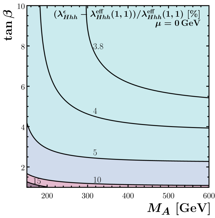
We show the Higgs self-coupling in Fig. 4 again for GeV, GeV and GeV. While the Higgs self-coupling obtained in the standard hMSSM approach shows large deviations from the exact value , the improved version , performs significantly better, compare Fig. 4 (a) and (d). The kinks at in Fig. 4 (d) are induced by our choice of , which is constant for and rescaled for . For non-vanishing the improved coupling shows remaining differences of a few percent, see Fig. 4 (e) and (f). This is not surprising, since a non-vanishing violates an assumption of the hMSSM approach: For GeV all entries in the correction of the -even Higgs mass matrix in Eq. (17) receive corrections. Still, we conclude that the improved couplings compared to show a milder spread when compared to the exact coupling throughout the --plane for all values of .
 |
|
|
| (a) | (b) | (c) |
 |
|
|
| (d) | (e) | (f) |
4.2 Momentum-dependent and kinetic corrections to
 |
 |
 |
| (a) | (b) | (c) |
Before we discuss the quality of the hMSSM approximation for what concerns we focus on the relevance of momentum-dependent and kinetic corrections for the partial decay width in the benchmark scenario with GeV. They arise from our Feynman-diagrammatic calculation with non-zero external momenta and the kinetic mixing discussed in Section 2.3, respectively. The total partial decay width for , , including all top-quark and stop corrections is depicted in Fig. 5 (a). First it is apparent that for low values of the heavy Higgs boson is too light to decay into a pair of two -even light Higgs bosons , such that the on-shell decay is kinematically closed. Only for low values of , where is decreasing rapidly, this decay mode is again of relevance. In all subsequent figures the region, where the on-shell decay is kinematically closed, is shown in white. We show the NLO partial decay width relative to the pure tree-level partial width including the tree-level Higgs self-coupling in Fig. 5 (b). We observe large corrections in accordance with the literature, see e.g. Ref. [48]. However, we point out that using the effective coupling in the tree-level decay width diminishes the one-loop corrections substantially, see Fig. 5 (c). Accordingly, Fig. 5 (c) demonstrates the relevance of the remaining momentum-dependent and kinetic corrections, which we incorporated through a Feynman-diagrammatic calculation and through the inclusion of the external kinetic mixing described in Section 2.3, respectively. Exactly such momentum-dependent and kinetic contributions were missing in the comparison of decay widths performed in Ref. [21]: Therein the partial decay width was compared against a full Feynman-diagrammatic one-loop calculation including an additional resummation of large logarithms. The discrepancies found at the level of the partial decay width in Ref. [21] were between % in a large part of the --plane and thus in the same ballpark as the missing momentum-dependent and kinetic contributions. Keep in mind that the partial decay width and thus the comparison in Ref. [21] missed also the constant factor between and . We leave a detailed comparison employing the newest predictions for a future study. We emphasize that the momentum-dependent and kinetic corrections in our benchmark scenario are mostly induced by the top-quark contribution, whereas the stops only yield a tiny fraction due to the relatively large stop masses. Given that in Fig. 5 we are not yet applying the hMSSM approximation similar results are obtained for larger values of . We therefore refrain from showing the corresponding results for GeV or GeV.
4.3 in the hMSSM
We finally focus on the performance of the hMSSM approximation in the description
of the partial decay width .
In Fig. 6 we compare the partial decay widths
and , both named option 2,
against the full result , named option 3 in Section 3.2.
In a first comparison we keep both top-quark and stop corrections in our calculation. For GeV
it is apparent, see Fig. 6 (a), that deviates from the exact
result by more than % for small values of . Using instead the improved Higgs self-coupling
in results in almost perfect agreement,
see Fig. 6 (d) with tiny deviations of only maximally %.
Choosing a non-vanishing value of , see Fig. 6 (b) and (c)
for GeV and GeV, respectively, leads to deviations
between the hMSSM prediction and
the exact result . Such
deviations increase with the value of
and follow a similar pattern as observed for
when compared against , see Fig. 4.
Keep in mind, that the squared value of enters the LO partial decay width.
Again the usage of , depicted in Fig. 6 (e) and (f),
makes the overall spread of the discrepancies between the hMSSM prediction
and the exact result smaller, but in particular for larger values of
they can still exceed %.
 |
|
|
| (a) | (b) | (c) |
 |
|
|
| (d) | (e) | (f) |
Lastly, we suggest to calculate in the hMSSM approach, since this calculation of the decay width incorporates the most dominant one-loop corrections from top quarks, but on the other hand is not sensitive to the actual supersymmetric spectrum and is thus in the spirit of the hMSSM approach. This decay width is compared against the exact result including top-quark and stop corrections in Fig. 7. From the fact that for small values there is only a small difference to the results including one-loop stop corrections , compare e.g. Fig. 6 (d) against Fig. 7 (a), we again conclude that momentum-dependent stop corrections are subdominant, at least for our benchmark scenario with stop masses above TeV and a heavy Higgs mass well below the TeV scale. The comparison of Fig. 6 (e) and (f) against Fig. 7 (b) and (c), respectively, shows that also for larger the momentum-dependent corrections from the stop sector can well be neglected.
 |
|
|
| (a) | (b) | (c) |
5 Conclusions
We revisited the calculation of the decay of the heavy Higgs boson into two SM-like Higgs bosons in the hMSSM approach. For this purpose we considered the full effective potential, in which the top quark and stops are integrated out, allowing to match the MSSM on a 2HDM as its low-energy limit. By carefully integrating out the top quark and stops separately, we identified missing contributions in the Higgs self-couplings of the hMSSM approach and suggested the definition of improved Higgs self-couplings for the hMSSM approximation. In particular in the limit of a small Higgsino mass parameter , which is an intrinsic assumption of the hMSSM approach, these improved Higgs self-couplings yield an excellent approximation for the actual Higgs self-couplings calculated in our effective potential approach. In this context the hMSSM approach can and has to be understood as an approximation to a full effective low-energy 2HDM matched to the MSSM. Since the effective potential is evaluated for zero external momenta, we included kinetic corrections at the level of the effective Lagrangian of the 2HDM involving dimension- operators. These corrections allow us to perform a one-loop Feynman-diagrammatic calculation of in the 2HDM-setup, where again we can consider the top quark and stops separately. By this procedure we discussed the relevance of momentum-dependent and kinetic corrections to the decay at the one-loop level, that were missing in previous comparisons. As for the Higgs self-couplings themselves using our improved Higgs self-couplings for the decay leads to a much better agreement between the calculation performed in the 2HDM-setup and the hMSSM approximation, in particular for small . We advocate to supplement the calculation of with momentum-dependent and kinetic corrections from the top quark to obtain a reliable prediction at one-loop level without introducing a dependence on the actual supersymmetric particle spectrum. Our study misses an inclusion of RGE effects, such that also heavier supersymmetric spectra can be investigated. We leave such comparisons to future work.
Acknowledgements
This work was inspired by comparisons performed in the context of the LHC Higgs XS working group. We thank Pietro Slavich for discussions. S.L. and M.M. are supported by the DFG project “Precision Calculations in the Higgs Sector - Paving the Way to the New Physics Landscape” (ID: MU 3138/1-1).
Appendix A Analytical results
We subsequently present the relevant analytical results, being the self-energies of the Higgs bosons and the virtual corrections to the vertex. We make use of Passarino-Veltman integrals [44, 45] to simplify our notation. For their presentation we need the Feynman rules for squark to Higgs-boson couplings, which we depict in Fig. 8. Note again that we work in the gaugeless limit, such that -term contributions to these couplings are neglected consistently. The couplings for the three-point interaction in Fig. 8 are given by ()
| (47) | ||||||
| (48) | ||||||
| (49) |
and for the four-point interaction by ()
| (50) |
Therein denotes the squark-mixing angle that diagonalizes the squark mass matrix in Eq. (9). Using from Eq. (19) the mixing angle can also be reexpressed as .
A.1 Vertex corrections
For the Feynman diagram involving the top-quark correction to , depicted in Fig. 1 (b), we obtain
| (51) |
where and we fix external momenta to the on-shell masses, i.e. . For the squark contributions we split the contribution from the Feynman diagram in Fig. 1 (c) from the sum of the contributions from the diagrams in Fig. 1 (d)–(f). For the former we obtain
| (52) |
and the sum of the diagrams in Fig. 1 (d)–(f) yields
| (53) |
where again external momenta are set on-shell. It is clear that is obtained by summing , while only consists of .
A.2 Self-energy corrections
Again we start with the top-quark contribution, which is depicted in Fig. 1 (l) and is given by
| (54) | ||||
| (55) |
where we attach two Higgs bosons externally. Finally for the sum of all stop contributions, shown in Fig. 1 (m, n), we obtain
| (56) | ||||
| (57) |
Again, and defined in Eq. (40) and Eq. (41), respectively, contain for only contributions from and and for in addition from and .
References
- [1] ATLAS, CMS Collaboration, G. Aad et al., Combined Measurement of the Higgs Boson Mass in Collisions at and 8 TeV with the ATLAS and CMS Experiments. Phys. Rev. Lett. 114 (2015) 191803, arXiv:1503.07589 [hep-ex].
- [2] ATLAS Collaboration Collaboration, G. Aad et al., Observation of a new particle in the search for the Standard Model Higgs boson with the ATLAS detector at the LHC. Phys.Lett. B716 (2012) 1–29, arXiv:1207.7214 [hep-ex].
- [3] CMS Collaboration Collaboration, S. Chatrchyan et al., Observation of a new boson at a mass of 125 GeV with the CMS experiment at the LHC. Phys.Lett. B716 (2012) 30–61, arXiv:1207.7235 [hep-ex].
- [4] Yu. A. Golfand and E. P. Likhtman, Extension of the Algebra of Poincare Group Generators and Violation of p Invariance. JETP Lett. 13 (1971) 323–326. [Pisma Zh. Eksp. Teor. Fiz.13,452(1971)].
- [5] D. Volkov and V. Akulov, Is the Neutrino a Goldstone Particle? Phys.Lett. B46 (1973) 109–110.
- [6] J. Wess and B. Zumino, Supergauge Transformations in Four-Dimensions. Nucl.Phys. B70 (1974) 39–50.
- [7] P. Fayet, Supergauge Invariant Extension of the Higgs Mechanism and a Model for the electron and Its Neutrino. Nucl. Phys. B90 (1975) 104–124.
- [8] P. Fayet, Spontaneously Broken Supersymmetric Theories of Weak, Electromagnetic and Strong Interactions. Phys. Lett. 69B (1977) 489.
- [9] P. Fayet and S. Ferrara, Supersymmetry. Phys. Rept. 32 (1977) 249–334.
- [10] H. P. Nilles, Supersymmetry, Supergravity and Particle Physics. Phys.Rept. 110 (1984) 1–162.
- [11] H. E. Haber and G. L. Kane, The Search for Supersymmetry: Probing Physics Beyond the Standard Model. Phys.Rept. 117 (1985) 75–263.
- [12] M. Sohnius, Introducing Supersymmetry. Phys.Rept. 128 (1985) 39–204.
- [13] J. Gunion and H. E. Haber, Higgs Bosons in Supersymmetric Models. 1. Nucl.Phys. B272 (1986) 1.
- [14] J. Gunion and H. E. Haber, Higgs Bosons in Supersymmetric Models. 2. Implications for Phenomenology. Nucl.Phys. B278 (1986) 449.
- [15] J. F. Gunion, H. E. Haber, G. L. Kane, and S. Dawson, The Higgs Hunter’s Guide. Front.Phys. 80 (2000) 1–448.
- [16] A. Djouadi, The Anatomy of electro-weak symmetry breaking. II. The Higgs bosons in the minimal supersymmetric model. Phys.Rept. 459 (2008) 1–241, arXiv:hep-ph/0503173 [hep-ph].
- [17] A. Djouadi, L. Maiani, G. Moreau, A. Polosa, J. Quevillon, and V. Riquer, The post-Higgs MSSM scenario: Habemus MSSM? Eur. Phys. J. C73 (2013) 2650, arXiv:1307.5205 [hep-ph].
- [18] A. Djouadi and J. Quevillon, The MSSM Higgs sector at a high : reopening the low tan regime and heavy Higgs searches. JHEP 10 (2013) 028, arXiv:1304.1787 [hep-ph].
- [19] L. Maiani, A. D. Polosa, and V. Riquer, Bounds to the Higgs Sector Masses in Minimal Supersymmetry from LHC Data. Phys. Lett. B724 (2013) 274–277, arXiv:1305.2172 [hep-ph].
- [20] A. Djouadi, L. Maiani, A. Polosa, J. Quevillon, and V. Riquer, Fully covering the MSSM Higgs sector at the LHC. JHEP 06 (2015) 168, arXiv:1502.05653 [hep-ph].
- [21] E. Bagnaschi et al., Benchmark scenarios for low in the MSSM. LHCHXSWG-2015-002 (2015) .
- [22] G. Lee and C. E. M. Wagner, Higgs bosons in heavy supersymmetry with an intermediate mA. Phys. Rev. D92 (2015) no. 7, 075032, arXiv:1508.00576 [hep-ph].
- [23] S. R. Coleman and E. J. Weinberg, Radiative Corrections as the Origin of Spontaneous Symmetry Breaking. Phys. Rev. D7 (1973) 1888–1910.
- [24] R. Jackiw, Functional evaluation of the effective potential. Phys. Rev. D9 (1974) 1686.
- [25] S. L. Adler, Axial vector vertex in spinor electrodynamics. Phys. Rev. 177 (1969) 2426–2438. [,241(1969)].
- [26] J. S. Bell and R. Jackiw, A PCAC puzzle: in the model. Nuovo Cim. A60 (1969) 47–61.
- [27] M. Beneke, P. Ruiz-Femenia, and M. Spinrath, Higgs couplings in the MSSM at large tan(beta). JHEP 01 (2009) 031, arXiv:0810.3768 [hep-ph].
- [28] L. J. Hall, R. Rattazzi, and U. Sarid, The Top quark mass in supersymmetric SO(10) unification. Phys. Rev. D50 (1994) 7048–7065, arXiv:hep-ph/9306309 [hep-ph].
- [29] Y. Okada, M. Yamaguchi, and T. Yanagida, Upper bound of the lightest Higgs boson mass in the minimal supersymmetric standard model. Prog. Theor. Phys. 85 (1991) 1–6.
- [30] H. E. Haber and R. Hempfling, Can the mass of the lightest Higgs boson of the minimal supersymmetric model be larger than m(Z)? Phys. Rev. Lett. 66 (1991) 1815–1818.
- [31] J. R. Ellis, G. Ridolfi, and F. Zwirner, Radiative corrections to the masses of supersymmetric Higgs bosons. Phys. Lett. B257 (1991) 83–91.
- [32] J. R. Ellis, G. Ridolfi, and F. Zwirner, On radiative corrections to supersymmetric Higgs boson masses and their implications for LEP searches. Phys. Lett. B262 (1991) 477–484.
- [33] A. Brignole, Radiative corrections to the supersymmetric neutral Higgs boson masses. Phys. Lett. B281 (1992) 284–294.
- [34] P. H. Chankowski, S. Pokorski, and J. Rosiek, Complete on-shell renormalization scheme for the minimal supersymmetric Higgs sector. Nucl. Phys. B423 (1994) 437–496, arXiv:hep-ph/9303309 [hep-ph].
- [35] A. Dabelstein, The One loop renormalization of the MSSM Higgs sector and its application to the neutral scalar Higgs masses. Z. Phys. C67 (1995) 495–512, arXiv:hep-ph/9409375 [hep-ph].
- [36] D. M. Pierce, J. A. Bagger, K. T. Matchev, and R.-J. Zhang, Precision corrections in the minimal supersymmetric standard model. Nucl. Phys. B491 (1997) 3–67, arXiv:hep-ph/9606211 [hep-ph].
- [37] V. D. Barger, M. S. Berger, A. L. Stange, and R. J. N. Phillips, Supersymmetric Higgs boson hadroproduction and decays including radiative corrections. Phys. Rev. D45 (1992) 4128–4147.
- [38] W. Hollik and S. Penaranda, Yukawa coupling quantum corrections to the selfcouplings of the lightest MSSM Higgs boson. Eur. Phys. J. C23 (2002) 163–172, arXiv:hep-ph/0108245 [hep-ph].
- [39] A. Dobado, M. J. Herrero, W. Hollik, and S. Penaranda, Selfinteractions of the lightest MSSM Higgs boson in the large pseudoscalar mass limit. Phys. Rev. D66 (2002) 095016, arXiv:hep-ph/0208014 [hep-ph].
- [40] M. Brucherseifer, R. Gavin, and M. Spira, Minimal supersymmetric Higgs boson self-couplings: Two-loop corrections. Phys. Rev. D90 (2014) no. 11, 117701, arXiv:1309.3140 [hep-ph].
- [41] M. Brucherseifer, Supersymmetric Higgs self-couplings: two-loop corrections. Dissertation, Zurich, ETH, 2012. http://e-collection.library.ethz.ch/view/eth:6693.
- [42] M. Carena, J. R. Espinosa, M. Quiros, and C. E. M. Wagner, Analytical expressions for radiatively corrected Higgs masses and couplings in the MSSM. Phys. Lett. B355 (1995) 209–221, arXiv:hep-ph/9504316 [hep-ph].
- [43] H. E. Haber, R. Hempfling, and A. H. Hoang, Approximating the radiatively corrected Higgs mass in the minimal supersymmetric model. Z. Phys. C75 (1997) 539–554, arXiv:hep-ph/9609331 [hep-ph].
- [44] G. ’t Hooft and M. J. G. Veltman, Scalar One Loop Integrals. Nucl. Phys. B153 (1979) 365–401.
- [45] G. Passarino and M. J. G. Veltman, One Loop Corrections for Annihilation Into in the Weinberg Model. Nucl. Phys. B160 (1979) 151–207.
- [46] A. Brignole and F. Zwirner, Radiative corrections to the decay in the minimal supersymmetric standard model. Phys. Lett. B299 (1993) 72–82, arXiv:hep-ph/9210266 [hep-ph].
- [47] T. Appelquist and J. Carazzone, Infrared Singularities and Massive Fields. Phys. Rev. D11 (1975) 2856.
- [48] K. E. Williams and G. Weiglein, Precise predictions for decays in the complex MSSM. Phys. Lett. B660 (2008) 217–227, arXiv:0710.5320 [hep-ph].
- [49] G. Chalons, A. Djouadi, and J. Quevillon, The neutral Higgs self-couplings in the (h)MSSM. Phys. Lett. B780 (2018) 74–80, arXiv:1709.02332 [hep-ph].
- [50] Particle Data Group Collaboration, Review of Particle Physics. Phys. Rev. D 98 (2018) 030001.