Fantom: A scalable framework for asynchronous distributed systems

In summary, this paper makes the following contributions:

• •

  We introduce the n-row flag table for faster root selection of the Lachesis Protocol.

• •

  We define continuous consistent cuts of a local view to achieve consensus.

• •

  We present proof of how domination relationships can be used for share information.

• •

  We formalize our proofs that can be applied to any generic asynchronous DAG solution.

The rest of this paper is organised as follows. Section 2 describes our Fantom framework. Section 3 presents the protocol implementation. Section 4 concludes. Proof of Byzantine fault tolerance is described in Section 5.2.

  (Lachesis) The set of protocols

  (Node) Each machine that participates in the Lachesis protocol is called a node. Let $n$ denote the total number of nodes.

  ($k$) A constant defined in the system.

  (Peer node) A node $n_{i}$ has $k$ peer nodes.

  (Process) A process $p_{i}$ represents a machine or a node. The process identifier of $p_{i}$ is $i$. A set $P$ = {1,…,$n$} denotes the set of process identifiers.

  (Channel) A process $i$ can send messages to process $j$ if there is a channel ($i$,$j$). Let $C$ $\subseteq$ {($i$,$j$) s.t. $i,j\in P$} denote the set of channels.

  (Event block) Each node can create event blocks, send (receive) messages to (from) other nodes.The structure of an event block includes the signature, generation time, transaction history, and hash information to references.

All nodes can create event blocks. The information of the referenced event blocks can be copied by each node. The first event block of each node is called a leaf event.

Suppose a node $n_{i}$ creates an event $v_{c}$ after an event $v_{s}$ in $n_{i}$. Each event block has exactly $k$ references. One of the references is self-reference, and the other $k$-1 references point to the top events of $n_{i}$’s $k$-1 peer nodes.

  (Top event) An event $v$ is a top event of a node $n_{i}$ if there is no other event in $n_{i}$ referencing $v$.

  (Height Vector) The height vector is the number of event blocks created by the $i$-th node.

  (In-degree Vector) The in-degree vector refers to the number of edges from other event blocks created by other nodes to the top event block of this node. The top event block indicates the most recently created event block by this node.

  (Ref) An event $v_{r}$ is called “ref” of event $v_{c}$ if the reference hash of $v_{c}$ points to the event $v_{r}$. Denoted by $v_{c}\hookrightarrow^{r}v_{r}$. For simplicity, we can use $\hookrightarrow$ to denote a reference relationship (either $\hookrightarrow^{r}$ or $\hookrightarrow^{s}$).

  (Self-ref) An event $v_{s}$ is called “self-ref” of event $v_{c}$, if the self-ref hash of $v_{c}$ points to the event $v_{s}$. Denoted by $v_{c}\hookrightarrow^{s}v_{s}$.

  ($k$ references) Each event block has at least $k$ references. One of the references is self-reference, and the other $k$-1 references point to the top events of $n_{i}$’s $k$-1 peer nodes.

  (Self-ancestor) An event block $v_{a}$ is self-ancestor of an event block $v_{c}$ if there is a sequence of events such that $v_{c}\hookrightarrow^{s}v_{1}\hookrightarrow^{s}\dots\hookrightarrow^{s}v_{m}\hookrightarrow^{s}v_{a}$. Denoted by $v_{c}\hookrightarrow^{sa}v_{a}$.

  (Ancestor) An event block $v_{a}$ is an ancestor of an event block $v_{c}$ if there is a sequence of events such that $v_{c}\hookrightarrow v_{1}\hookrightarrow\dots\hookrightarrow v_{m}\hookrightarrow v_{a}$. Denoted by $v_{c}\hookrightarrow^{a}v_{a}$.

For simplicity, we simply use $v_{c}\hookrightarrow^{a}v_{s}$ to refer both ancestor and self-ancestor relationship, unless we need to distinguish the two cases.

  (Flag Table) The flag table is a $n\times k$ matrix, where $n$ is the number of nodes and k is the number of roots that an event block can reach. If an event block $e$ created by $i$-th node can reach $j$-th root, then the flag table stores the hash value of the $j$-th root.

Our Lachesis protocols relies on Lamport timestamps to define a topological ordering of event blocks in OPERA chain. By using Lamport timestamps, we do not rely on physical clocks to determine a partial ordering of events.

The “happened before” relation, denoted by $\rightarrow$, gives a partial ordering of events from a distributed system of nodes. Each node $n_{i}$ (also called a process) is identified by its process identifier $i$. For a pair of event blocks $v$ and $v^{\prime}$, the relation ”$\rightarrow$” satisfies: (1) If $v$ and $v^{\prime}$ are events of process $P_{i}$, and $v$ comes before $v^{\prime}$, then $b\rightarrow v^{\prime}$. (2) If $v$ is the send($m$) by one process and $v^{\prime}$ is the receive($m$) by another process, then $v\rightarrow v^{\prime}$. (3) If $v\rightarrow v^{\prime}$ and $v^{\prime}\rightarrow v^{\prime\prime}$ then $v\rightarrow v^{\prime\prime}$. Two distinct events $v$ and $v^{\prime}$ are said to be concurrent if $v\nrightarrow v^{\prime}$ and $v^{\prime}\nrightarrow v$.

For an arbitrary total ordering $\prec$ of the processes, a relation $\Rightarrow$ is defined as follows: if $v$ is an event in process $P_{i}$ and $v^{\prime}$ is an event in process $P_{j}$, then $v\Rightarrow v^{\prime}$ if and only if either (i) $C_{i}(v)<C_{j}(v^{\prime})$ or (ii) $C(v)=C_{j}(v^{\prime})$ and $P_{i}\prec P_{j}$. This defines a total ordering, and that the Clock Condition implies that if $v\rightarrow v^{\prime}$ then $v\Rightarrow v^{\prime}$.

We use this total ordering in our Lachesis protocol. This ordering is used to determine consensus time, as described in Section 3.

  (Happened-Immediate-Before) An event block $v_{x}$ is said Happened-Immediate-Before an event block $v_{y}$ if $v_{x}$ is a (self-) ref of $v_{y}$. Denoted by $v_{x}\mapsto v_{y}$.

  (Happened-before) An event block $v_{x}$ is said Happened-Before an event block $v_{y}$ if $v_{x}$ is a (self-) ancestor of $v_{y}$. Denoted by $v_{x}\rightarrow v_{y}$.

Happened-before is the relationship between nodes which have event blocks. If there is a path from an event block $v_{x}$ to $v_{y}$, then $v_{x}$ Happened-before $v_{y}$. “$v_{x}$ Happened-before $v_{y}$” means that the node creating $v_{y}$ knows event block $v_{x}$. This relation is the transitive closure of happens-immediately-before. Thus, an event $v_{x}$ happened before an event $v_{y}$ if one of the followings happens: (a) $v_{y}\hookrightarrow^{s}v_{x}$, (b) $v_{y}\hookrightarrow^{r}v_{x}$, or (c) $v_{y}\hookrightarrow^{a}v_{x}$. The happened-before relation of events form an acyclic directed graph $G^{\prime}=(V,E^{\prime})$ such that an edge $(v_{i},v_{j})\in E^{\prime}$ has a reverse direction of the same edge in $E$.

  (Concurrent) Two event blocks $v_{x}$ and $v_{y}$ are said concurrent if neither of them happened before the other. Denoted by $v_{x}\parallel v_{y}$.

Given two vertices $v_{x}$ and $v_{y}$ both contained in two OPERA chains (DAGs) $G_{1}$ and $G_{2}$ on two nodes. We have the following:

1. (1)

   $v_{x}\rightarrow v_{y}$ in $G_{1}$ if $v_{x}\rightarrow v_{y}$ in $G_{2}$.

2. (2)

   $v_{x}\parallel v_{y}$ in $G_{1}$ if $v_{x}\parallel v_{y}$ in $G_{2}$.

Each node has a local state, a collection of histories, messages, event blocks, and peer information, we describe the components of each.

  (State) A state of a process $i$ is denoted by $s_{j}^{i}$.

  (Local State) A local state consists of a sequence of event blocks $s_{j}^{i}=v_{0}^{i},v_{1}^{i},\dots,v_{j}^{i}$.

In a DAG-based protocol, each $v_{j}^{i}$ event block is valid only if the reference blocks exist before it. From a local state $s_{j}^{i}$, one can reconstruct a unique DAG. That is, the mapping from a local state $s_{j}^{i}$ into a DAG is injective or one-to-one. Thus, for Fantom, we can simply denote the $j$-th local state of a process $i$ by the DAG $g_{j}^{i}$ (often we simply use $G_{i}$ to denote the current local state of a process $i$).

  (Action) An action is a function from one local state to another local state.

Generally speaking, an action can be one of: a $send(m)$ action where $m$ is a message, a $receive(m)$ action, and an internal action. A message $m$ is a triple $\langle i,j,B\rangle$ where $i\in P$ is the sender of the message, $j\in P$ is the message recipient, and $B$ is the body of the message. Let $M$ denote the set of messages. In the Lachesis protocol, $B$ consists of the content of an event block $v$.

Semantics-wise, in Lachesis, there are two actions that can change a process’s local state: creating a new event and receiving an event from another process.

  (Event) An event is a tuple $\langle s,\alpha,s^{\prime}\rangle$ consisting of a state, an action, and a state. Sometimes, the event can be represented by the end state $s^{\prime}$.

The $j$-th event in history $h_{i}$ of process $i$ is $\langle s_{j-1}^{i},\alpha,s_{j}^{i}\rangle$, denoted by $v_{j}^{i}$.

  (Local history) A local history $h_{i}$ of process $i$ is a (possibly infinite) sequence of alternating local states — beginning with a distinguished initial state. A set $H_{i}$ of possible local histories for each process $i$ in $P$.

The state of a process can be obtained from its initial state and the sequence of actions or events that have occurred up to the current state. In the Lachesis protocol, we use append-only semantics. The local history may be equivalently described as either of the following:

In Lachesis, a local history is equivalently expressed as:

where $g_{j}^{i}$ is the $j$-th local DAG (local state) of the process $i$.

  (Run) Each asynchronous run is a vector of local histories. Denoted by $\sigma=\langle h_{1},h_{2},h_{3},...h_{N}\rangle$.

Let $\Sigma$ denote the set of asynchronous runs. We can now use Lamport’s theory to talk about global states of an asynchronous system. A global state of run $\sigma$ is an $n$-vector of prefixes of local histories of $\sigma$, one prefix per process. The happens-before relation can be used to define a consistent global state, often termed a consistent cut, as follows.

Consistent cuts represent the concept of scalar time in distributed computation, it is possible to distinguish between a “before” and an “after”.

In the Lachesis protocol, an OPERA chain $G=(V,E)$ is a directed acyclic graph (DAG). $V$ is a set of vertices and $E$ is a set of edges. DAG is a directed graph with no cycle. There is no path that has source and destination at the same vertex. A path is a sequence of vertices ($v_{1}$, $v_{2}$, …, $v_{k-1}$, $v_{k}$) that uses no edge more than once.

An asynchronous system consists of the following sets: a set $P$ of process identifiers; a set $C$ of channels; a set $H_{i}$ is the set of possible local histories for each process $i$; a set $A$ of asynchronous runs; a set $M$ of all messages.

Each process / node in Lachesis selects $k$ other nodes as peers. For certain gossip protocol, nodes may be constrained to gossip with its $k$ peers. In such a case, the set of channels $C$ can be modelled as follows. If node $i$ selects node $j$ as a peer, then $(i,j)\in C$. In general, one can express the history of each node in DAG-based protocol in general or in Lachesis protocol in particular, in the same manner as in the CCK paper [9].

  (Consistent cut) A consistent cut of a run $\sigma$ is any global state such that if $v_{x}^{i}\rightarrow v_{y}^{j}$ and $v_{y}^{j}$ is in the global state, then $v_{x}^{i}$ is also in the global state. Denoted by $\mathbf{c}(\sigma)$.

The concept of consistent cut formalizes such a global state of a run. A consistent cut consists of all consistent DAG chains. A received event block exists in the global state implies the existence of the original event block. Note that a consistent cut is simply a vector of local states; we will use the notation $\mathbf{c}(\sigma)[i]$ to indicate the local state of $i$ in cut $\mathbf{c}$ of run $\sigma$.

A message chain of an asynchronous run is a sequence of messages $m_{1}$, $m_{2}$, $m_{3}$, $\dots$, such that, for all $i$, $receive(m_{i})$ $\rightarrow$ $send(m_{i+1})$. Consequently, $send(m_{1})$ $\rightarrow$ $receive(m_{1})$ $\rightarrow$ $send(m_{2})$ $\rightarrow$ $receive(m_{2})$ $\rightarrow$ $send(m_{3})$ $\dots$.

The formal semantics of an asynchronous system is given via the satisfaction relation $\vdash$. Intuitively $\mathbf{c}(\sigma)\vdash\phi$, “$\mathbf{c}(\sigma)$ satisfies $\phi$,” if fact $\phi$ is true in cut $\mathbf{c}$ of run $\sigma$.

We assume that we are given a function $\pi$ that assigns a truth value to each primitive proposition $p$. The truth of a primitive proposition $p$ in $\mathbf{c}(\sigma)$ is determined by $\pi$ and $\mathbf{c}$. This defines $\mathbf{c}(\sigma)\vdash p$.

  (Equivalent cuts) Two cuts $\mathbf{c}(\sigma)$ and $\mathbf{c^{\prime}}(\sigma^{\prime})$ are equivalent with respect to $i$ if:

  ($i$ knows $\phi$) $K_{i}(\phi)$ represents the statement “$\phi$ is true in all possible consistent global states that include $i$’s local state”.

  ($i$ partially knows $\phi$) $P_{i}(\phi)$ represents the statement “there is some consistent global state in this run that includes $i$’s local state, in which $\phi$ is true.”

  (Majority concurrently knows) The next modal operator is written $M^{C}$ and stands for “majority concurrently knows.” The definition of $M^{C}(\phi)$ is as follows.

where $S\subseteq P$ and $|S|>2n/3$.

This is adapted from the “everyone concurrently knows” in CCK paper [9]. In the presence of one-third of faulty nodes, the original operator “everyone concurrently knows” is sometimes not feasible. Our modal operator $M^{C}(\phi)$ fits precisely the semantics for BFT systems, in which unreliable processes may exist.

  (Concurrent common knowledge) The last modal operator is concurrent common knowledge (CCK), denoted by $C^{C}$. $C^{C}(\phi)$ is defined as a fixed point of $M^{C}(\phi\wedge X)$.

CCK defines a state of process knowledge that implies that all processes are in that same state of knowledge, with respect to $\phi$, along some cut of the run. In other words, we want a state of knowledge $X$ satisfying: $X=M^{C}(\phi\wedge X)$. $C^{C}$ will be defined semantically as the weakest such fixed point, namely as the greatest fixed-point of $M^{C}(\phi\wedge X)$.It therefore satisfies:

Thus, $P_{i}(\phi)$ states that there is some cut in the same asynchronous run $\sigma$ including $i$’s local state, such that $\phi$ is true in that cut.

Note that $\phi$ implies $P_{i}(\phi)$. But it is not the case, in general, that $P_{i}(\phi)$ implies $\phi$ or even that $M^{C}(\phi)$ implies $\phi$. The truth of $M^{C}(\phi)$ is determined with respect to some cut $\mathbf{c}(\sigma)$. A process cannot distinguish which cut, of the perhaps many cuts that are in the run and consistent with its local state, satisfies $\phi$; it can only know the existence of such a cut.

  (Global fact) Fact $\phi$ is valid in system $\Sigma$, denoted by $\Sigma\vdash\phi$, if $\phi$ is true in all cuts of all runs of $\Sigma$.

Fact $\phi$ is valid, denoted $\vdash\phi$, if $\phi$ is valid in all systems, i.e. $(\forall\Sigma)(\Sigma\vdash\phi)$.

  (Local fact) A fact $\phi$ is local to process $i$ in system $\Sigma$ if $\Sigma\vdash(\phi\Rightarrow K_{i}\phi)$.

In a graph $G=(V,E,r)$ a dominator is the relation between two vertices. A vertex $v$ is dominated by another vertex $w$, if every path in the graph from the root $r$ to $v$ have to go through $w$. Furthermore, the immediate dominator for a vertex $v$ is the last of $v$’s dominators, which every path in the graph have to go through to reach $v$.

  (Pseudo top) A pseudo vertex, called top, is the parent of all top event blocks. Denoted by $\top$.

  (Pseudo bottom) A pseudo vertex, called bottom, is the child of all leaf event blocks. Denoted by $\bot$.

With the pseudo vertices, we have $\bot$ happened-before all event blocks. Also all event blocks happened-before $\top$. That is, for all event $v_{i}$, $\bot\rightarrow v_{i}$ and $v_{i}\rightarrow\top$.

  (Dom) An event $v_{d}$ dominates an event $v_{x}$ if every path from $\top$ to $v_{x}$ must go through $v_{d}$. Denoted by $v_{d}\gg v_{x}$.

  (Strict dom) An event $v_{d}$ strictly dominates an event $v_{x}$ if $v_{d}\gg v_{x}$ and $v_{d}$ does not equal $v_{x}$. Denoted by $v_{d}\gg^{s}v_{x}$.

  (Domfront) A vertex $v_{d}$ is said “domfront” a vertex $v_{x}$ if $v_{d}$ dominates an immediate predecessor of $v_{x}$, but $v_{d}$ does not strictly dominate $v_{x}$. Denoted by $v_{d}\gg^{f}v_{x}$.

  (Dominance frontier) The dominance frontier of a vertex $v_{d}$ is the set of all nodes $v_{x}$ such that $v_{d}\gg^{f}v_{x}$. Denoted by $DF(v_{d})$.

From the above definitions of domfront and dominance frontier, the following holds. If $v_{d}\gg^{f}v_{x}$, then $v_{x}\in DF(v_{d})$.

The core idea of the Lachesis protocol is to use a DAG-based structure, called the OPERA chain for our consensus algorithm. In the Lachesis protocol, a (participant) node is a server (machine) of the distributed system. Each node can create messages, send messages to, and receive messages from, other nodes. The communication between nodes is asynchronous.

Let $n$ be the number of participant nodes. For consensus, the algorithm examines whether an event block is dominated by $2n/3$ nodes, where $n$ is the number of all nodes. The Happen-before relation of event blocks with $2n/3$ nodes means that more than two-thirds of all nodes in the OPERA chain know the event block.

The OPERA chain (DAG) is the local view of the DAG held by each node, this local view is used to identify topological ordering, select Clotho, and create time consensus through Atropos selection. OPERA chain is a DAG graph $G=(V,E)$ consisting of $V$ vertices and $E$ edges. Each vertex $v_{i}\in V$ is an event block. An edge $(v_{i},v_{j})\in E$ refers to a hashing reference from $v_{i}$ to $v_{j}$; that is, $v_{i}\hookrightarrow v_{j}$.

  (Leaf) The first created event block of a node is called a leaf event block.

  (Root) The leaf event block of a node is a root. When an event block $v$ can reach more than $2n/3$ of the roots in the previous frames, $v$ becomes a root.

  (Root set) The set of all first event blocks (leaf events) of all nodes form the first root set $R_{1}$ ($|R_{1}|$ = $n$). The root set $R_{k}$ consists of all roots $r_{i}$ such that $r_{i}$ $\not\in$ $R_{i}$, $\forall$ $i$ = 1..($k$-1) and $r_{i}$ can reach more than 2n/3 other roots in the current frame, $i$ = 1..($k$-1).

  (Frame) Frame $f_{i}$ is a natural number that separates Root sets. The root set at frame $f_{i}$ is denoted by $R_{i}$.

  (Consistent chains) OPERA chains $G_{1}$ and $G_{2}$ are consistent if for any event $v$ contained in both chains, $G_{1}[v]=G_{2}[v]$. Denoted by $G_{1}\sim G_{2}$.

When two consistent chains contain the same event $v$, both chains contain the same set of ancestors for $v$, with the same reference and self-ref edges between those ancestors.

If two nodes have OPERA chains containing event $v$, then they have the same $k$ hashes contained within $v$. A node will not accept an event during a sync unless that node already has $k$ references for that event, so both OPERA chains must contain $k$ references for $v$. The cryptographic hashes are assumed to be secure, therefore the references must be the same. By induction, all ancestors of $v$ must be the same. Therefore, the two OPERA chains are consistent.

  (Creator) If a node $n_{x}$ creates an event block $v$, then the creator of $v$, denoted by $cr(v)$, is $n_{x}$.

  (Consistent chain) A global consistent chain $G^{C}$ is a chain if $G^{C}\sim G_{i}$ for all $G_{i}$.

We denote $G\sqsubseteq G^{\prime}$ to stand for $G$ is a subgraph of $G^{\prime}$. Some properties of $G^{C}$ are given as follows:

1. (1)

   $\forall G_{i}$ ($G^{C}\sqsubseteq G_{i}$).

2. (2)

   $\forall v\in G^{C}$ $\forall G_{i}$ ($G^{C}[v]\sqsubseteq G_{i}[v]$).

3. (3)

   ($\forall v_{c}\in G^{C}$) ($\forall v_{p}\in G_{i}$) (($v_{p}\rightarrow v_{c})\Rightarrow v_{p}\in G^{C}$).

  (Consistent root) Two chains $G_{1}$ and $G_{2}$ are root consistent, if for every $v$ contained in both chains, $v$ is a root of $j$-th frame in $G_{1}$, then $v$ is a root of $j$-th frame in $G_{2}$.

By consistent chains, if $G_{1}\sim G_{2}$ and $v$ belongs to both chains, then $G_{1}[v]$ = $G_{2}[v]$. We can prove the proposition by induction. For $j$ = 0, the first root set is the same in both $G_{1}$ and $G_{2}$. Hence, it holds for $j$ = 0. Suppose that the proposition holds for every $j$ from 0 to $k$. We prove that it also holds for $j$= $k$ + 1. Suppose that $v$ is a root of frame $f_{k+1}$ in $G_{1}$. Then there exists a set $S$ reaching 2/3 of members in $G_{1}$ of frame $f_{k}$ such that $\forall u\in S$ ($u\rightarrow v$). As $G_{1}\sim G_{2}$, and $v$ in $G_{2}$, then $\forall u\in S$ ($u\in G_{2}$). Since the proposition holds for $j$=$k$, As $u$ is a root of frame $f_{k}$ in $G_{1}$, $u$ is a root of frame $f_{k}$ in $G_{2}$. Hence, the set $S$ of 2/3 members $u$ happens before $v$ in $G_{2}$. So $v$ belongs to $f_{k+1}$ in $G_{2}$.

Thus, all nodes have the same consistent root sets, which are the root sets in $G^{C}$. Frame numbers are consistent for all nodes.

  (Flag table) A flag table stores reachability from an event block to another root. The sum of all reachabilities, namely all values in flag table, indicates the number of reachabilities from an event block to other roots.

  (Consistent flag table) For any top event $v$ in both OPERA chains $G_{1}$ and $G_{2}$, and $G_{1}\sim G_{2}$, then the flag tables of $v$ are consistent if they are the same in both chains.

From the above, the root sets of $G_{1}$ and $G_{2}$ are consistent. If $v$ contained in $G_{1}$, and $v$ is a root of $j$-th frame in $G_{1}$, then $v$ is a root of $j$-th frame in $G_{i}$. Since $G_{1}\sim G_{2}$, $G_{1}[v]=G_{2}[v]$. The reference event blocks of $v$ are the same in both chains. Thus the flag tables of $v$ of both chains are the same.

  (Clotho) A root $r_{k}$ in the frame $f_{a+3}$ can nominate a root $r_{a}$ as Clotho if more than 2n/3 roots in the frame $f_{a+1}$ dominate $r_{a}$ and $r_{k}$ dominates the roots in the frame $f_{a+1}$.

Each node nominates a root into Clotho via the flag table. If all nodes have an OPERA chain with same shape, the values in flag table will be equal to each other in OPERA chain. Thus, all nodes nominate the same root into Clotho since the OPERA chain of all nodes has same shape.

  (Atropos) An Atropos is assigned consensus time through the Lachesis consensus algorithm and is utilized for determining the order between event blocks. Atropos blocks form a Main-chain, which allows time consensus ordering and responses to attacks.

For any root set $R$ in the frame $f_{i}$, the time consensus algorithm checks whether more than 2n/3 roots in the frame $f_{i-1}$ selects the same value. However, each node selects one of the values collected from the root set in the previous frame by the time consensus algorithm and Reselection process. Based on the Reselection process, the time consensus algorithm can reach agreement. However, there is a possibility that consensus time candidate does not reach agreement [10]. To solve this problem, time consensus algorithm includes minimal selection frame per next $h$ frame. In minimal value selection algorithm, each root selects minimum value among values collected from previous root set. Thus, the consensus time reaches consensus by time consensus algorithm.

  (Main-chain (Blockchain)) For faster consensus, Main-chain is a special sub-graph of the OPERA chain (DAG).

The Main chain — a core subgraph of OPERA chain, plays the important role of ordering the event blocks. The Main chain stores shortcuts to connect between the Atropos. After the topological ordering is computed over all event blocks through the Lachesis protocol, Atropos blocks are determined and form the Main chain. To improve path searching, we use a flag table — a local hash table structure as a cache that is used to quickly determine the closest root to a event block.

In the OPERA chain, an event block is called a root if the event block is linked to more than two-thirds of previous roots. A leaf vertex is also a root itself. With root event blocks, we can keep track of “vital” blocks that $2n/3$ of the network agree on.

Figure 2 shows an example of the Main chain composed of Atropos event blocks. In particular, the Main chain consists of Atropos blocks that are derived from root blocks and so are agreed by $2n/3$ of the network nodes. Thus, this guarantees that at least $2n/3$ of nodes have come to consensus on this Main chain.

Each participant node has a copy of the Main chain and can search consensus position of its own event blocks. Each event block can compute its own consensus position by checking the nearest Atropos event block. Assigning and searching consensus position are introduced in the consensus time selection section.

The Main chain provides quick access to the previous transaction history to efficiently process new incoming event blocks. From the Main chain, information about unknown participants or attackers can be easily viewed. The Main chain can be used efficiently in transaction information management by providing quick access to new event blocks that have been agreed on by the majority of nodes. In short, the Main-chain gives the following advantages:

- All event blocks or nodes do not need to store all information. It is efficient for data management.

- Access to previous information is efficient and fast.

Based on these advantages, OPERA chain can respond strongly to efficient transaction treatment and attacks through its Main-chain.

In order to create an event block, a node needs to select $k$ other nodes. Lachesis protocols does not depend on how peer nodes are selected. One simple approach can use a random selection from the pool of $n$ nodes. The other approach is to define some criteria or cost function to select other peers of a node.

Within distributed system, a node can select other nodes with low communication costs, low network latency, high bandwidth, high successful transaction throughputs.

Our Lachesis protocol allows an arbitrary number of participants to dynamically join the system. The OPERA chain (DAG) can still operate with new participants. Computation on flag tables is set based and independent of which and how many participants have joined the system. Algorithms for selection of Roots, Clothos and Atroposes are flexible enough and not dependence on a fixed number of participants.

We describe an algorithm that synchronizes events between the nodes.

The algorithm assumes that a node always needs the events in topological ordering (specifically in reference to the lamport timestamps), an alternative would be to use an inverse bloom lookup table (IBLT) for completely potential randomized events.

Alternatively, one can simply use a fixed incrementing index to keep track of the top event for each node.

This section gives an overview of the node structure in Lachesis.

Each node has a height vector, in-degree vector, flag table, frames, clotho check list, max-min value, main-chain (blockchain), and their own local view of the OPERA chain (DAG). The height vector is the number of event blocks created by the $i$-th node. The in-degree vector refers to the number of edges from other event blocks created by other nodes to the top event block of this node. The top event block indicates the most recently created event block by this node. The flag table is a $nxk$ matrix, where n is the number of nodes and k is the number of roots that an event block can reach. If an event block $e$ created by $i$-th node can reach $j$-th root, then the flag table stores the hash value of the $j$-th root. Each node maintains the flag table of each top event block.

Frames store the root set in each frame. Clotho check list has two types of check points; Clotho candidate ($CC$) and Clotho ($C$). If a root in a frame is a $CC$, a node check the $CC$ part and if a root becomes Clotho, a node check $C$ part. Max-min value is timestamp that addresses for Atropos selection. The Main-chain is a data structure storing hash values of the Atropos blocks.

Figure 3 shows an example of the node structure component of a node $A$. In the figure, each value excluding self height in the height vector is 1 since the initial state is shared to all nodes. In the in-degree vector, node $A$ stores the number of edges from other event blocks created by other nodes to the top event block. The in-degrees of node $A$, $B$, and $C$ are 1. In flag table, node $A$ knows other two root hashes since the top event block can reach those two roots. Node $A$ also knows that other nodes know their own roots. In the example situation there is no clotho candidate and Clotho, and thus clotho check list is empty. The main-chain and max-min value are empty for the same reason as clotho check list.

We define three versions of the Cost Function ($C_{F}$). Version one is focused around updated information share and is discussed below. The other two versions are focused on root creation and consensus facilitation, these will be discussed in a following paper.

We define a Cost Function ($C_{F}$) for preventing the creation of lazy nodes. A lazy node is a node that has a lower work portion in the OPERA chain (has created fewer event blocks). When a node creates an event block, the node selects other nodes with low value outputs from the cost function and refers to the top event blocks of the reference nodes. An equation (1) of $C_{F}$ is as follows,

where $I$ and $H$ denote values of in-degree vector and height vector respectively. If the number of nodes with the lowest $C_{F}$ is more than $k$, one of the nodes is selected at random. The reason for selecting high $H$ is that we can expect a high possibility to create a root because the high $H$ indicates that the communication frequency of the node had more opportunities than others with low $H$. Otherwise, the nodes that have high $C_{F}$ (the case of $I$ $>$ $H$) have generated fewer event blocks than the nodes that have low $C_{F}$..

Figure 4 shows an example of the node selection based on the cost function after the creation of leaf events by all nodes. In this example, there are five nodes and each node created leaf events. All nodes know other leaf events. Node $A$ creates an event block $v_{1}$ and $A$ calculates the cost functions. Step 2 in Figure 4 shows the results of cost functions based on the height and in-degree vectors of node $A$. In the initial step, each value in the vectors are same because all nodes have only leaf events. Node $A$ randomly selects $k$ nodes and connects $v_{1}$ to the leaf events of selected nodes. In this example, we set $k$=3 and assume that node $A$ selects node $B$ and $C$.

Figure 5 shows an example of the node selection after a few steps of the simulation in Figure 4. In Figure 5, the recent event block is $v_{5}$ created by node $A$. Node $A$ calculates the cost function and selects the other two nodes that have the lowest results of the cost function. In this example, node $B$ has 0.5 as the result and other nodes have the same values. Because of this, node $A$ first selects node $B$ and randomly selects other nodes among nodes $C$, $D$, and $E$.

The height of node $D$ in the example is 2 (leaf event and event block $v_{4}$). On the other hand, the height of node $D$ in node structure of $A$ is 1. Node $A$ is still not aware of the presence of the event block $v_{4}$. It means that there is no path from the event blocks created by node $A$ to the event block $v_{4}$. Thus, node $A$ has 1 as the height of node $D$.

Algorithm 3 shows the selecting algorithm for selecting reference nodes. The algorithm operates for each node to select a communication partner from other nodes. Line 4 and 5 set min_cost and $S_{ref}$ to initial state. Line 7 calculates the cost function $c_{f}$ for each node. In line 8, 9, and 10, we find the minimum value of the cost function and set min_cost and $S_{ref}$ to $c_{f}$ and the ID of each node respectively. Line 11 and 12 append the ID of each node to $S_{ref}$ if min_cost equals $c_{f}$. Finally, line 13 selects randomly $k$ node IDs from $S_{ref}$ as communication partners. The time complexity of Algorithm 2 is $O(n)$, where $n$ is the number of nodes.

After the reference node is selected, each node communicates and shares information of all event blocks known by them. A node creates an event block by referring to the top event block of the reference node. The Lachesis protocol works and communicates asynchronously. This allows a node to create an event block asynchronously even when another node creates an event block. The communication between nodes does not allow simultaneous communication with the same node.

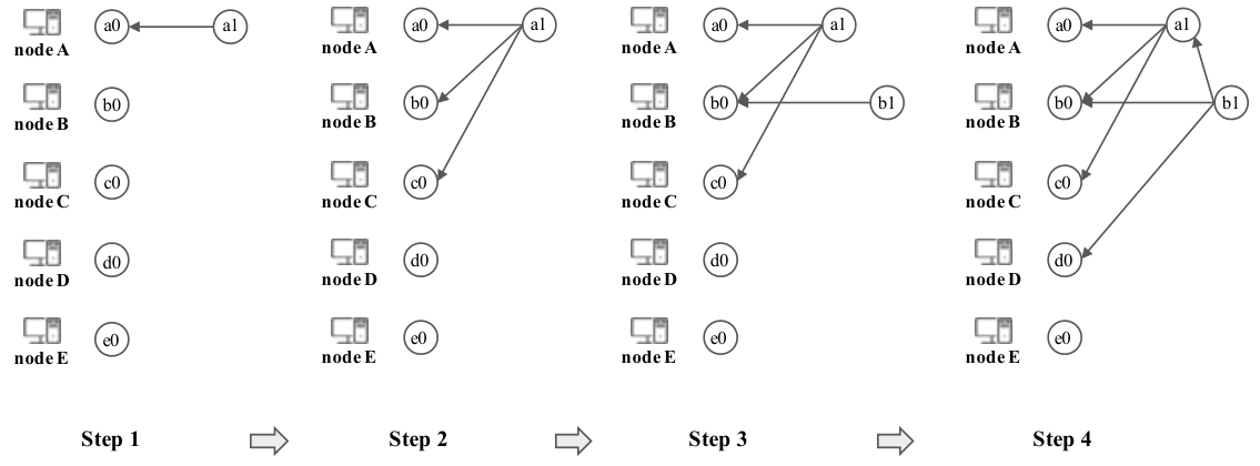
Figure 6 shows an example of the node selection in Lachesis protocol. In this example, there are five nodes ($A,B,C,D,$ and $E$) and each node generates the first event blocks, called leaf events. All nodes share other leaf events with each other. In the first step, node $A$ generates new event block $a_{1}$. Then node $A$ calculates the cost function to connect other nodes. In this initial situation, all nodes have one event block called leaf event, thus the height vector and the in-degree vector in node $A$ has same values. In other words, the heights of each node are 1 and in-degrees are 0. Node $A$ randomly select the other two nodes and connects $a_{1}$ to the top two event blocks from the other two nodes. Step 2 shows the situation after connections. In this example, node $A$ select node $B$ and $C$ to connect $a_{1}$ and the event block $a_{1}$ is connected to the top event blocks of node $B$ and $C$. Node $A$ only knows the situation of the step 2.

After that, in the example, node $B$ generates a new event block $b_{1}$ and also calculates the cost function. $B$ randomly select the other two nodes; $A$, and $D$, since $B$ only has information of the leaf events. Node $B$ requests to $A$ and $D$ to connect $b_{1}$, then nodes $A$ and $D$ send information for their top event blocks to node $B$ as response. The top event block of node $A$ is $a_{1}$ and node $D$ is the leaf event. The event block $b_{1}$ is connected to $a_{1}$ and leaf event from node $D$. Step 4 shows these connections.

In the Lachesis protocol, every node can create an event block. Each event block refers to other $k$ event blocks using their hash values. In the Lachesis protocol, a new event block refers to $k$-neighbor event blocks under the following conditions:

1. 1.

   Each of the $k$ reference event blocks is the top event blocks of its own node.

2. 2.

   One reference should be made to a self-ref that references to an event block of the same node.

3. 3.

   The other $k$-1 reference refers to the other $k$-1 top event nodes on other nodes.

Figure 7 shows the example of an event block creation with a flag table. In this example the recent created event block is $b_{1}$ by node $B$. The figure shows the node structure of node $B$. We omit the other information such as height and in-degree vectors since we only focus on the change of the flag table with the event block creation in this example. The flag table of $b_{1}$ in Figure 7 is updated with the information of the previous connected event blocks $a_{1}$, $b_{0}$, and $c_{1}$. Thus, the set of the flag table is the results of OR operation among the three root sets for $a1$ ($a_{0}$, $b_{0}$, and $c_{0}$), $b_{0}$ ($b_{0}$), and $c_{1}$ ($b_{0}$, $c_{0}$, and $d_{0}$).

Figure 8, shows the communication process is divided into five steps for two nodes to create an event block. Simply, a node $A$ requests to $B$. then, $B$ responds to $A$ directly.

Every node has a physical clock and it needs physical time to create an event block. However, for consensus, Lachesis protocols relies on a logical clock for each node. For the purpose, we use ”Lamport timestamps” [11] to determine the time ordering between event blocks in a asynchronous distributed system.

The Lamport timestamps algorithm is as follows:

1. 1.

   Each node increments its count value before creating an event block.

2. 2.

   When sending a message include its count value, receiver should consider which sender’s message is received and increments its count value.

3. 3.

   If current counter is less than or equal to the received count value from another node, then the count value of the recipient is updated.

4. 4.

   If current counter is greater than the received count value from another node, then the current count value is updated.

We use the Lamport’s algorithm to enforce a topological ordering of event blocks and use it in the Atropos selection algorithm.

Since an event block is created based on logical time, the sequence between each event blocks is immediately determined. Because the Lamport timestamps algorithm gives a partial order of all events, the whole time ordering process can be used for Byzantine fault tolerance.

Here, we introduce a new idea that extends the concept of domination.

For a vertex $v$ in a DAG $G$, let $G[v]=(V_{v},E_{v})$ denote an induced-subgraph of $G$ such that $V_{v}$ consists of all ancestors of $v$ including $v$, and $E_{v}$ is the induced edges of $V_{v}$ in $G$.

For a set $S$ of vertices, an event $v_{d}$ $\frac{2}{3}$-dominates $S$ if there are more than 2/3 of vertices $v_{x}$ in $S$ such that $v_{d}$ dominates $v_{x}$. Recall that $R_{1}$ is the set of all leaf vertices in $G$. The $\frac{2}{3}$-dom set $D_{0}$ is the same as the set $R_{1}$.The $\frac{2}{3}$-dom set $D_{i}$ is defined as follows:

A vertex $v_{d}$ belongs to a $\frac{2}{3}$-dom set within the graph $G[v_{d}]$, if $v_{d}$ $\frac{2}{3}$-dominates $R_{1}$. The $\frac{2}{3}$-dom set $D_{k}$ consists of all roots $d_{i}$ such that $d_{i}$ $\not\in$ $D_{i}$, $\forall$ $i$ = 1..($k$-1), and $d_{i}$ $\frac{2}{3}$-dominates $D_{i-1}$.

The $\frac{2}{3}$-dom set $D_{i}$ is the same with the root set $R_{i}$, for all nodes.

This section gives several examples of DAGs and the domination relation between their event blocks.

Figure 10 shows an examples of a DAG and dominator trees.

Figure 11 depicts an example of a DAG and 2/3 dom sets.

Figure 12 shows an example an dependency graphs. On each row, the left most figure shows the latest OPERA chain. The left figures on each row depict the dependency graphs of each node, which are in their compact form. When no fork presents, each of the compact dependency graphs is a tree.

Figure 13 shows an example of a pair of fork events. Each row shows an OPERA chain (left most) and the compact dependency graphs on each node (right). The fork events are shown in red and green vertices

All nodes can create event blocks and an event block can be a root when satisfying specific conditions. Not all event blocks can be roots. First, the first created event blocks are themselves roots. These leaf event blocks form the first root set $R_{S_{1}}$ of the first frame $f_{1}$. If there are total $n$ nodes and these nodes create the event blocks, then the cardinality of the first root set $|R_{S_{1}}|$ is $n$. Second, if an event block $e$ can reach at least 2n/3 roots, then $e$ is called a root. This event $e$ does not belong to $R_{S1}$, but the next root set $R_{S_{2}}$ of the next frame $f_{2}$. Thus, excluding the first root set, the range of cardinality of root set $R_{S_{k}}$ is $2n/3<|R_{S_{k}}|\leq n$. The event blocks including $R_{S_{k}}$ before $R_{S_{k+1}}$ is in the frame $f_{k}$. The roots in $R_{S_{k+1}}$ does not belong to the frame $f_{k}$. Those are included in the frame $f_{k+1}$ when a root belonging to $R_{S_{k+2}}$ occurs.

We introduce the use of a flag table to quickly determine whether a new event block becomes a root. Each node maintains a flag table of the top event block. Every event block that is newly created is assigned $k$ hashes for its $k$ referenced event blocks. We apply an $OR$ operation on each set in the flag table of the referenced event blocks.

Figure 14 shows an example of how to use flag tables to determine a root. In this example, $b_{1}$ is the most recently created event block. We apply an $OR$ operation on each set of the flag tables for $b_{1}$’s $k$ referenced event blocks. The result is the flag table of $b_{1}$. If the cardinality of the root set in $b_{1}$’s flag table is more than $2n/3$, $b_{1}$ is a root. In this example, the cardinality of the root set in $b_{1}$ is 4, which is greater than $2n/3$ ($n$=5). Thus, $b_{1}$ becomes root. In this example, $b_{1}$ is added to frame $f_{2}$ since $b_{1}$ becomes new root.

The root selection algorithm is as follows:

1. 1.

   The first event blocks are considered as roots.

2. 2.

   When a new event block is added in the OPERA chain (DAG), we check whether the event block is a root by applying an $OR$ operation on each set of the flag tables connected to the new event block. If the cardinality of the root set in the flag table for the new event block is more than 2n/3, the new event block becomes a root.

3. 3.

   When a new root appears on the OPERA chain, nodes update their frames. If one of the new event blocks becomes a root, all nodes that share the new event block add the hash value of the event block to their frames.

4. 4.

   The new root set is created if the cardinality of the previous root set $R_{S_{p}}$ is more than 2n/3 and the new event block can reach $2n/3$ roots in $R_{S_{p}}$.

5. 5.

   When the new root set $R_{S_{k+1}}$ is created, the event blocks from the previous root set $R_{S_{k}}$ to before $R_{S_{k+1}}$ belong to the frame $f_{k}$.

A Clotho is a root that satisfies the Clotho creation conditions. Clotho creation conditions are that more than 2n/3 nodes know the root and a root knows this information.

In order for a root $r$ in frame $f_{i}$ to become a Clotho, $r$ must be reached by more than n/3 roots in the frame $f_{i+1}$. Based on the definition of the root, each root reaches more than 2n/3 roots in previous frames. If more than n/3 roots in the frame $f_{i+1}$ can reach $r$, then $r$ is spread to all roots in the frame $f_{i+2}$. It means that all nodes know the existence of $r$. If we have any root in the frame $f_{i+3}$, a root knows that $r$ is spread to more than 2n/3 nodes. It satisfies Clotho creation conditions.

In the example in Figure 15, n is 5 and each circle indicates a root in a frame. Each arrow means one root can reach (happened-before) to the previous root. Each root has 4 or 5 arrows (out-degree) since n is 5 (more than 2n/3 $\geq$ 4). $b_{1}$ and $c_{2}$ in frame $f_{2}$ are roots that can reach $c_{0}$ in frame $f_{1}$. $d_{1}$ and $e_{1}$ also can reach $c_{0}$, but we only marked $b_{1}$ and $c_{2}$ (when n is 5, more than n/3 $\geq$ 2) since we show at least more than n/3 conditions in this example. And it was marked with a blue bold arrow (Namely, the roots that can reach root $c_{0}$ have the blue bold arrow). In this situation, an event block must be able to reach $b_{1}$ or $c_{2}$ in order to become a root in frame $f_{3}$ (In our example, n=5, more than n/3 $\geq$ 2, and more than 2n/3 $\geq$ 4. Thus, to be a root, either must be reached). All roots in frame $f_{3}$ reach $c_{0}$ in frame $f_{1}$.

To be a root in frame $f_{4}$, an event block must reach more than 2n/3 roots in frame $f_{3}$ that can reach $c_{0}$. Therefore, if any of the root in frame $f_{4}$ exists, the root must have happened-before more than 2n/3 roots in frame $f_{3}$. Thus, the root of $f_{4}$ knows that $c_{0}$ is spread over more than 2n/3 of the entire nodes. Thus, we can select $c_{0}$ as Clotho.

Figure 16 shows an example of a Clotho. In this example, all roots in the frame $f_{1}$ have happened-before more than n/3 roots in the frame $f_{2}$. We can select all roots in the frame $f_{1}$ as Clotho since the recent frame is $f_{4}$.

Algorithm 4 shows the pseudo code for Clotho selection. The algorithm takes a root $r$ as input. Line 4 and 5 set $c.is\_clotho$ and $c.yes$ to $nil$ and 0 respectively. Line 6-8 checks whether any root $c^{\prime}$ in $frame(i-3,r)$ has happened-before with the 2n/3 condition $c$ where $i$ is the current frame. In line 9-10, if the number of roots in $frame(i-2,r)$ which happened-before $c$ is more than $2n/3$, the root $c$ is set as a Clotho. The time complexity of Algorithm 3 is $O(n^{2})$, where $n$ is the number of nodes.

Figure 17 shows the state of node A when a Clotho is selected. In this example, node A knows all roots in the frame $f_{1}$ become Clotho’s. Node A prunes unnecessary information on its own structure. In this case, node A prunes the root set in the frame $f_{1}$ since all roots in the frame $f_{1}$ become Clotho and the Clotho Check list stores the Clotho information.

Atropos selection algorithm is the process in which the candidate time generated from Clotho selection is shared with other nodes, and each root re-selects candidate time repeatedly until all nodes have same candidate time for a Clotho.

After a Clotho is nominated, each node then computes a candidate time of the Clotho. If there are more than two-thirds of the nodes that compute the same value for candidate time, that time value is recorded. Otherwise, each node reselects candidate time. By the reselection process, each node reaches time consensus for candidate time of Clotho as the OPERA chain (DAG) grows. The candidate time reaching the consensus is called Atropos consensus time. After Atropos consensus time is computed, the Clotho is nominated to Atropos and each node stores the hash value of Atropos and Atropos consensus time in Main-Chain (blockchain). The Main-chain is used for time order between event blocks. The proof of Atropos consensus time selection is shown in the section 5.2.

Figure 18 shows the example of Atropos selection. In Figure 16, all roots in the frame $f_{1}$ are selected as Clotho through the existence of roots in the frame $f_{4}$. Each root in the frame $f_{5}$ computes candidate time using timestamps of reachable roots in the frame $f_{4}$. Each root in the frame $f_{5}$ stores the candidate time to min-max value space. The root $r_{6}$ in the frame $f_{6}$ can reach more than 2n/3 roots in $f_{5}$ and $r_{6}$ can know the candidate time of the reachable roots that $f_{5}$ takes. If $r_{6}$ knows the same candidate time than more than 2n/3, we select the candidate time as Atropos consensus time. Then all Clotho in the frame $f_{1}$ become Atropos.

Figure 19 shows the state of node B when Atropos is selected. In this example, node B knows all roots in the frame $f_{1}$ become Atropos. Then node B prunes information of the frame $f_{1}$ in clotho check list since all roots in the frame $f_{1}$ become Atropos and main chain stores Atropos information.