Experimental Quantum Switching for Exponentially Superior Quantum Communication Complexity
Abstract
Finding exponential separation between quantum and classical information tasks is like striking gold in quantum information research. Such an advantage is believed to hold for quantum computing but is proven for quantum communication complexity. Recently, a novel quantum resource called the quantum switch—which creates a coherent superposition of the causal order of events, known as quantum causality—has been harnessed theoretically in a new protocol providing provable exponential separation. We experimentally demonstrate such an advantage by realizing a superposition of communication directions for a two-party distributed computation. Our photonic demonstration employs -dimensional quantum systems, qudits, up to dimensions and demonstrates a communication complexity advantage, requiring less than times the communication of any causally ordered protocol. These results elucidate the crucial role of the coherence of communication direction in achieving the exponential separation for the one-way processing task, and open a new path for experimentally exploring the fundamentals and applications of advanced features of indefinite causal structures.
Computation by separated parties with minimal communication is the focus of communication complexity, which has applications to distributed computing, very-large-scale integration, streaming algorithms, and more Buhrman et al. 2010. For quantum information, communication complexity is especially exciting as exponential quantum-classical gaps can be proven Yao 1979; Brassard 2003; Raz 1999; Buhrman et al. 2001; Bar-Yossef et al. 2004; Gavinsky et al. 2007; Regev and Klartag 2011; Arrazola and Lütkenhaus 2014. By contrast, exponential quantum-classical gaps for computation tasks such as factorization Shor 1999 depend on the best-known classical algorithm, and thus are strongly believed but not rigorously proven. Experimentally, quantum communication complexity has been studied in proof of principle for the quantum fingerprinting protocol Horn et al. 2005; Xu et al. 2015; Guan et al. 2016 and beyond Buhrman et al. 2010; Du et al. 2006; Trojek et al. 2005.
The quantum switch provides a new communication complexity tool that leads to another instance of exponential quantum advantage Guérin et al. 2016. The quantum switch is a device where a control qubit determines the order in which two transformations are performed on a target system Oreshkov et al. 2012; Chiribella et al. 2013. When the control is in a superposition of logical states, the order of the operations is causally indefinite; i.e., there is a superposition of the ordering of target operations. The quantum switch has broad relevance in the context of quantum causality Brukner 2014 including applications to studies of quantum gravity Hardy 2007; Zych et al.; Brukner 2014; Rubino et al., communication complexity Feix et al. 2015; Guérin et al. 2016, witnessing causality Oreshkov et al. 2012; Araújo et al. 2015; Branciard et al. 2015; Rubino et al. 2017; Goswami et al. 2018; Castro-Ruiz et al. 2018 and deciding whether a given indefinite causal order is physical Araújo et al. 2017; Oreshkov. In quantum computing, the quantum switch can reduce the query complexity for some tasks compared to causally ordered protocols Chiribella et al. 2013; Araújo et al. 2014 — this advantage has been demonstrated for single-qubit control and single-qubit target circuits Procopio et al. 2015. In quantum communication, the quantum switch enhances the communication rate beyond the limits of conventional quantum Shannon theory Ebler et al. 2018; Goswami et al..
In this letter, we demonstrate a quantum-switch-based exponentially enhanced quantum-communication protocol, modified from a recent theory proposal Guérin et al. 2016. We implement a single-qubit-controlled switch acting on a target Hilbert space of dimensions realized as a qudit Bartlett et al. 2002; Patera and Zassenhaus 1988, which simplifies the experiment compared to using multiple qubits while maintaining the Hilbert-space dimension. Unlike past experimental qubit implementations Procopio et al. 2015; Rubino et al. 2017; Goswami et al. 2018; Rubino et al.; Goswami et al., our experiment provides the first demonstration of the quantum switch involving a qudit target system.
The communication task that we consider is known as the exchange evaluation (EE) game, illustrated in Fig. 1. For bit strings and Boolean functions , Alice and Bob receive inputs and , respectively, such that , with being the all-zero string. Another party, Charlie, must compute the exchange evaluation function subject to the one-way communication condition that Alice and Bob can each send a system to the outside environment only once. They are thus forbidden to communicate back and forth by sending quantum or classical systems to each other at different time steps.

Guérin proposed a protocol that uses the superposition of the communication direction between Alice and Bob to solve the EE game with unit success probability, using an amount of communication that scales exponentially better with the input bit string size compared to any causally ordered protocol Guérin et al. 2016. They cast the task in terms of the problem of deciding whether two unitary operations, which depend on the inputs of Alice and Bob, commute or anticommute. This constitutes precisely the question that can be solved efficiently with the quantum switch. Importantly, the communication complexity advantage is not limited to the ideal case of deterministic answers, which are unachievable in any real experiment; it also survives for the more practical bounded-error case. Despite the elegance of the protocol in theory, it is challenging in experiment because the protocol typically requires the manipulation of more than 10 entangled qubits to enter the regime where the causally indefinite advantage starts.
We implement a variant of the protocol that renders it experimentally feasible with current technology (see Appendix A and B). In our protocol, we use a quantum switch where one qubit acts as the control, and the target system is a -dimensional qudit Bartlett et al. 2002 with , thus making it equivalent to entangled qubits. We implement both systems with a single photon by encoding the control system in the path degree of freedom and the target system in the arrival time of the photon, which is divided into a set of time bins forming the basis . Consistent with the notation for , we write and as the unary representations of the bit strings and , respectively, noting that the maximum value they can take is . To account for the different dimensionality of the target system and these bit strings (See Appendix A), we trivially augment the functions and as for .
Our protocol tests whether two unitary operators and commute or anticommute when applied to a particular target state. The relationship between this task and the communication complexity one (evaluating ) can be seen by representing and in the unitary-operator basis given by the generalized Pauli operators Bartlett et al. 2002; Patera and Zassenhaus 1988 and satisfying . In this basis, we write and define and . Thus,
| (1) |
where t denotes the target system.
The quantum switch can be used to solve this problem as follows (see Fig. 1). The control qubit is prepared in the state , and the target system is initialized in . After applying the unitary operators and to the target system in the order determined by the control qubit, a Hadamard gate is applied to the control qubit, with the resulting state of the overall system being . Then, a measurement of the control qubit by Charlie in the computational basis reveals whether or , which completes the communication-complexity task.
To implement the protocol, the state preparation and the Hadamard gate for the control qubit encoded in the path degree of freedom are realized using a beam splitter (BS). The target qubit initialization in is equivalent to the photon starting in the first time bin. The transformations and are implemented as delays by time bins in Alice’s laboratory and time bins in Bob’s laboratory, respectively. Furthermore, is implemented in Alice’s laboratory using a phase modulator that applies the appropriate phase (0 if or if ) to each time bin, with a corresponding implementation for in Bob’s laboratory.
The experiment utilities a fiber-based Sagnac interferometer, shown in Fig. 2. A heralded single photon, generated by type-II spontaneous parametric down-conversion, passes a circulator and then enters the Sagnac loop, via a BS, in a superposition of two directions. Alice and Bob each possess a variable delay line and a time-dependent phase modulator to realize the unitary transformations and , respectively. They each implement the transformation once on the component of the photon that passes through them after entering the loop, and once more on the component that passes through them before exiting the loop. Depending on the binary answer to the EE game, the photon interferes such that it exits at one or the other of the two interferometer outputs. The outputs are monitored by two high-quality superconducting nanowire single-photon detectors (SNSPDs). The detection events are registered using a time-to-digital converter.

In the experimental implementation of the communication complexity protocol, the amount of communication and the error probability are to be minimized. These goals lead to three main technological challenges (see Appendix C). (i) Precise timing is required to ensure that the correct phase is imparted at the second station. We use a sequence of home-made fiber segments to create the choices of delays for each of Alice and Bob with a high accuracy, and a 25-GHz arbitrary waveform generator, triggered by the heralding signal, in such a way that the modulation timing accurately coincides with the time bins (of length 2 ns) of the heralded photons. (ii) To minimize noise, we use two SNSPDs with ultralow dark-count rates below Hz, and perform careful temperature control and polarization control to maximize the interference visibility. (iii) It requires the optimization of the efficiency throughout the setup, to minimize the amount of required communication. For example, we need a loss dB to beat the classical definite protocol with . To this end, we choose suitable pump and detection beam waists for the down-conversion process, use custom-made low-loss components in the Sagnac loop, and detect the photons with high-efficiency SNSPDs.
In our experiment, we determine the error probability and the transmitted information for each . We record two-photon coincidence counts (between SNSPD1 and either SNSPD2 or SNSPD3) ( Fig. 2). We estimate the error probability (i.e. the probability of an incorrect result) focusing on two important cases: the worst case, where both Alice and Bob have the largest input (corresponding to the largest delays and system loss); and the one-bit-different case where Alice changes the choice of the -th segment, , while Bob holds the largest input. The goal of testing the second case is to verify that the delay of each segment is well made, so that Alice has the ability to implement any of the possible delays. Figure 3 shows the detailed experimental error probability for , where we obtained a value of for the worst case (red bar). As expected, for other values of , the error probability is below that of the worst case. For other values of , see the Appendix D.
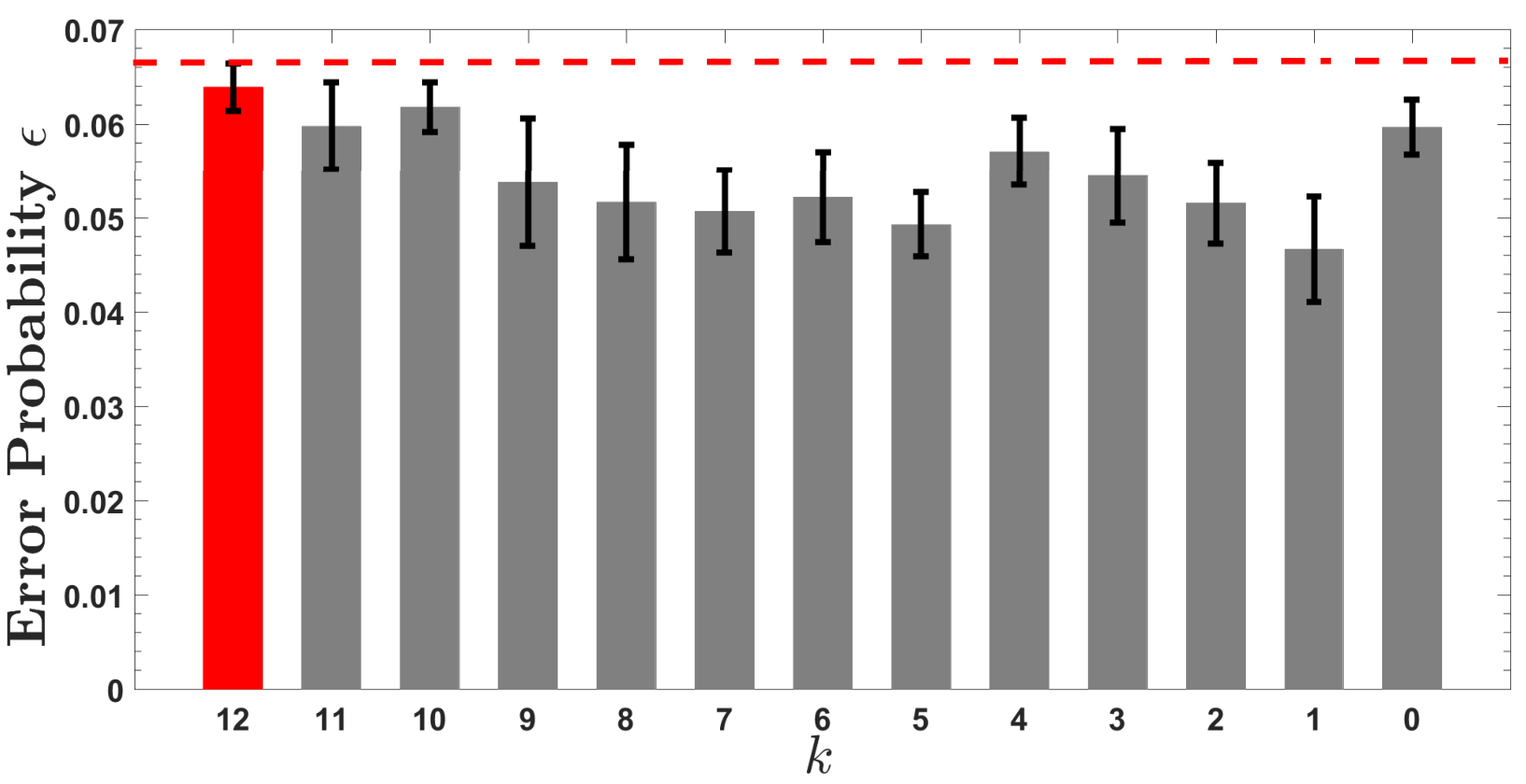

Figure 4 shows the experimental transmitted information required to complete the task for different system sizes. We compare our protocol with a bound for classical protocols (black solid curve) and a bound for quantum causally definite protocols (blue solid curve). A lower bound on the transmitted information in any classical protocol, allowing for a bounded error probability of , is , where is the binary entropy. Any quantum causally definite protocol needs to transmit at least , half as much as classical protocols Guérin et al. 2016. We use the worst-case () to calculate the minimum transmitted information of classical and quantum causally definite protocols, because it gives the most stringent bound to beat. For each , the transmitted information of our protocol is estimated to be , where () denotes the worst-case overall system efficiency for the given system size. Figure 4 indicates that, with increasing system size , the causally indefinite protocol provides an exponential advantage in the scaling of transmitted information. In particular, for , the experimental results clearly beat all classical protocols as well as all quantum causally definite protocols.
To further quantify our results, we define as the ratio between the transmitted information of our causally indefinite protocol, and the minimum transmitted information of a given type of causally ordered protocol (either classical or quantum causally definite): . In Fig. 4, we plot the experimental results for as a function of different protocols and different input sizes. Figure 4 shows that our protocol requires the transmission of only of the information of any classical protocol and of the information of any causally definite quantum protocol.
Our experimental results show that we have demonstrated the EE game, even taking into account small experimental imperfections. First, we measured the second-order correlation function at zero delay of our heralded single-photon source, and obtained , where the error bars represent 1 standard deviation. The value is close to 0, which ensures the condition of one-way communication in EE game, as discussed in Guérin et al. 2016; Procopio et al. 2015(see Appendix C.5). Second, the random choice of the delay and the phase modulation were carefully characterized (see Tab. S1 in C), which guaranteed the implementation of arbitrary bit inputs (,) and functions (, ), as required by the EE game. Third, although the error probability is rising with increasing system size, by careful optimizing the setup, the results of Fig. 3 show that the error probability is below a tolerable range. Such a small error is sufficient to realize the EE game with causally indefinite quantum protocol. Fourth, though the optical loss is exponential growth with the increasing system size, the results of Fig. 4 prove that with system sizes of 13 bits, we can access the regime where our causally indefinite quantum protocol outperforms any causally definite protocol.
Overall, we have experimentally demonstrated that the superposition of communication direction can provide an exponential reduction of communication complexity. We achieve this through the use of a high-dimensional degree of freedom, the photon arrival time. Although our temporal qudit encoding is not efficiently scalable to very large , our experiment elucidates the crucial role of coherence in achieving the exponential separation between quantum and classical communication in a distributed processing task. Decoherence would destroy the superposition of communication directions—reverting to a situation where it is necessary to transmit the function itself through the one-way channel to achieve deterministic two-party function evaluation. Our results establish that the quantum switch can serve as a powerful resource in quantum communication, which may provide a new paradigm of Shannon theory, where the order of the communication channels can be in a quantum superposition, and therefore strongly motivates further experimental development with qudit or other encodings.
Acknowledgements.
This work was supported by the National Key R&D Program of China (Grant No. SQ2018YFB0504303, SQ2018YFB050101), the National Natural Science Foundation of China (Grants No. 61771443 and No. 61705048), the Chinese Academy of Sciences, the Thousand Young Talent Program of China, Shanghai Science and Technology Development Funds (Grant No. 18JC1414700), and the Australian Research Council (Grant No. DP160101911). The authors would like to thank Norbert Lütkenhaus, Farzad Ghafari, Jian-Yu Guan, and Cheng Wu for helpful discussions.Appendix A Comparison of our protocol with that of Ref. Guérin et al. 2016
Our protocol differs slightly from the original scheme proposed in Ref. Guérin et al. 2016. The unitary transformation was originally proposed in terms of modulo-two addition, as . Our definition of retains the key property of , while being experimentally much more readily realizable. Note that the fact that our target system is equivalent to qubits as opposed to the qubits of Ref. Guérin et al. 2016 is not a fundamental consequence of the time-bin implementation. One could also have the target system corresponding to qubits, and use the transformation . Such a permutation would require using fast switches in addition to the delays, as shown in Fig. 5.
Appendix B Practical considerations
Our encoding of the whole multi-qubit system in a single photon entails both benefits and drawbacks. It is beneficial given the presence of probabilistic photon loss, an unavoidable experimental imperfection. Efficiency is a crucial factor in demonstrating the advantage provided by the quantum switch, and presents one of the main technical challenges of the experiment. Loss is detrimental because it effectively requires the repetition of the protocol, thereby increasing the communication, while the performance is benchmarked against optimal lossless causally ordered protocols. As a result of our implementation, our quantum system is only subjected to the probabilistic loss associated with one photon. However, the encoding of the target qubits in the photon arrival time also leads to an exponential growth of the number of required time bins as a function of the number of target qubits. This practically limits the ability to scale the protocol to an arbitrarily high value of . Nevertheless, our experiment proves that it is possible to access the regime where our causally indefinite quantum protocol outperforms any causally definite protocol.
In contrast to previous communication complexity experiments on quantum fingerprinting that were based on coherent states Xu et al. 2015; Guan et al. 2016, we use single photons in this experiment. The use of coherent states would arguably violate a rule of the exchange evaluation game, namely that Alice and Bob are each only allowed to receive a system from the outside environment once. As a test of one-way communication, Ref.Guérin et al. 2016 proposed having a (hypothetical) counter in each laboratory that is incremented by one whenever a system enters the laboratory. Our single photon constitutes an indivisible quantum system, so the meaning of “a system entering” is unambiguous, and the counters would read one at the end of the protocol, in agreement with the rules of the game. However, for the case of a coherent state divided on a beam splitter, each component could be considered a quantum system on its own. In that case, the counters would read two, in violation of the rules of the game. It has recently also been experimentally shown that the use of single photons can enable secure communication with a hidden communication direction Del Santo and Dakić 2018; Massa et al..
The coherence length of our source is approximately several centimeters, which does not cover the whole switch. For our setup, having a coherence length that covers the whole interferometer is not an option. First, we have an extremely long path in the interferometer and it is extremely challenging to have a narrow-bandwidth single photon source. Second, we use time-bin encoding so our photon must be contained in a time bin for modulation – the coherence length must be shorter than the separation between bins.
It is also worth noting that an indefinite causal order has been formally witnessed elsewhere without the use of an especially narrowband single photon Rubino et al. 2017.

Appendix C Experimental details
C.1 Heralded single-photon source
The photon pairs are produced via type-II spontaneous parametric down-conversion. The pump light is emitted by a 780-nm continuous-wave laser diode (LD). After passing through a 945-nm short-pass filter (945SP) used to remove the residual long wavelengths from outside fluorescence, the pump light is focused into a 10 mm, periodically poled potassium titanyl phosphate (PPKTP) crystal to convert pump photons into pairs of orthogonally polarized photons at a wavelength of 1560 nm. The down-converted photons are separated by a polarizing beam splitter (PBS), and the residual pump light is removed by two filters. The down-converted photons are then coupled into single-mode fibers with a 76.9% coupling efficiency. One of them passes a circulator before entering the Sagnac loop. To herald the presence of the correlated photon, the other one is directly detected by a high-quality superconducting nanowire single-photon detector (SNSPD1) with 80.6% detection efficiency. Overall, the heralding efficiency is approximately , including all losses in the photon-pair source setup (but excluding the elements used to implement the communication complexity protocol).
C.2 Sagnac loop
The Sagnac loop is depicted in Fig. 2 of the main text. A 50:50 beam splitter (BS) is used to create the superposition of communication direction. Alice and Bob each possess a variable delay and a phase modulator to implement their unitary operators based on their inputs when the photon arrives at their stations. The unitaries consist of phase modulations followed by delays. However, because and the photon is initialized in the first time bin, no phase modulation needs to be implemented at the first station, only the delays. The photon then continues along the Sagnac loop, through a 7 km fiber spool in which the pulse trains are stored, and to the second station. There, Alice and Bob each implement their phase modulation, followed by their delay. Finally, the two paths interfere at the BS and the photon is detected by two high-quality SNSPDs (SNSPD2 with a detection efficiency of 76.5% and dark count rate of 9.3 Hz, SNSPD3 with a detection efficiency of 72.0% and a dark count rate of 8.3 Hz). The two-photon coincidences are registered by a time-to-digital converter (TDC). All components in the loop have ultra-low insertion loss to minimize the communication complexity.
C.3 Dark counts
The coincidence time window in the causally indefinite protocol is very large. In contrast to typical two-photon coincidence experiments where the coincidence window tends to be a few ns, in the causally indefinite protocol, the heralding photon arrives in a given time bin while the heralded photon can be in one of time bins. This means that the coincidence time window is ns for the given 2 ns time bin, orders of magnitude larger than that in normal two-photon coincidence detection. If there is a dark count during this time (or a subset of this interval when applying gating), it will be erroneously registered as an event. To suppress dark counts due to thermal background radiation, we use two high-quality SNSPDs that use a low-loss bandpass filter. The SNSPDs can detect photons with an ultra-low dark-count rate of Hz and a high detection efficiency of .
C.4 Losses
To minimize the experimental communication in the causally indefinite protocol, the experimental setup should have as small a loss as possible. Here, three strategies are applied to minimize the total loss of the setup. First, for the heralded single-photon source, by setting the pump beam waist to , the detection beam waist at the center of the PPKTP crystal to , and by heralding the daughter photons using a high-quality SNSPD (detection efficiency of 80.6%, dark count rate of 11.0 Hz), we achieve a high heralding efficiency of , corresponding to 2.07 dB loss in the source. Second, in the Sagnac loop, all components are custom-made to achieve ultra-low loss. As discussed in Section E of this Supplemental Material, instead of using highly lossy optical switches, we implement the delay by joining the different fiber segments via mating sleeves. There, we use different connector types, SC/PC to FC/PC mating sleeves (Thorlabs), which provide a lower loss ( dB), compared with a typical loss of FC/PC to FC/PC mating sleeves ( dB). As a result, for each system size , we implement the delays with extremely low loss. Lastly, for the detection we use two high-quality SNSPDs that have a high detection efficiency of 72.0% and 76.5% together with an ultra-low dark count rate of 8.3 Hz and 9.3 Hz, respectively. The overall system loss, excluding the loss of the variable delays in Alice and Bob’s stations, is 11.62 dB.
C.5 Measurement of the second-order correlation function
We need to demonstrate that a pure single photon are used, as this is underlying assumptionGuérin et al. 2016. This can be shown by measuring the second-order correlation function at zero delay of our heralded single-photon source, . For an ideal heralded single-photon source, the value of is 0, which implies that only a single photon is sent to the Sagnac loop each time. To measure , in the same way as for the scheme in Ref. U’Ren et al. 2005; Jin et al. 2015, we simply steer one of the outputs of the beam splitter (in Fig. 2 of the main text) to SNSPD2, and the other one to SNSPD3. Since the pump light is emitted by a continuous-wave LD, we register all detection events by the TDC and post-select the coincidence events. is evaluated with the following equation:
| (2) |
where is the single count of SNSPD1; and are two-fold concidence rate between SNSPD1 and SNSPD2, and between SNSPD1 and SNSPD3, respectively; denotes the three-fold coincidence rate of SNSPD1, SNSPD2 and SNSPD3.
At our pump power of 3 mW,we average the count rates over 5 minutes, obtaining , where the error bars represent 1 standard deviation, following Poisson statistics. The value is very close to 0, which means that an almost perfect single-photon source is used in our experiment. Hence, similarly to Ref. Procopio et al. 2015; Guérin et al. 2016, using the hypothetical photon-counter scheme where we place a counters at the output ports of Alice’s and Bob’s station to read the number of uses of channel, we would see that the counters of Alice and Bob are 1, which means that the channel is used only once.
C.6 Implementation of the unitary transformations
For our protocol, Alice (Bob) needs to realize one of the possible delays, depending on her (his) input bit string, and guarantee that her (his) PM correctly modulates the photon after the delay from Bob (Alice). Therefore, after the delay, the photon pulse must be fully contained in the appropriate time bin. Instead of using highly lossy switches, we implement the variable delays with segments of fiber, where for the -th segment, there is a choice of two fibers that have a length difference equivalent to a delay of time bins, , as illustrated in Fig. 6. We use a 25 GHz arbitrary waveform generator (Tektronix70002), which is triggered by the heralding signal, to generate a modulation pulse sequence with a pulse width of 2 ns. The rising edge and the falling edge of the pulse are ps. The delay between the heralding signal and the modulation pulse is accurately controlled such that the heralded photon is positioned in the middle of the first time bin.

The time delay of commercial off-the-shelf fiber spools is measured using a conventional optical time domain reflectometer (OTDR). By itself, it has a low accuracy and does not meet the sensitivity demands of our experiment. For example, the distance uncertainty of a conventional state-of-the-art OTDR (Exfo FTB7600E) is meter, corresponding to a time-delay uncertainty of ns, where is the length of the fiber spool and is group velocity in fiber. In our experiment, we home made all the fiber segments with a time-delay uncertainty of ps using the following method:
- 1.
To make one of the segments whose time delay is ns, we cut off a ns time-delay fiber with an FC/PC connector at one end and an SC bare fiber terminator (Thorlabs) at the other end, using a commercial OTDR to approximate the length. For the segments whose time delay is in the event dead zone of the OTDR, we directly make it by using a ruler with a resolution of 0.5 mm (= 2.5 ps).
- 2.
We measure the time delay of the segment using our home-built photon-counting OTDR variant shown in Fig. 7, which achieves a resolution of 1 ps. Then, we cleave the redundant fiber whose length is measured by a ruler with a resolution of 0.5 mm (= 2.5 ps).
- 3.
We pull the fiber out the bare fiber terminator. Then the fiber is connectorised and is slightly polished with an SC/FC connector achieving a low insertion loss.
The resultant length of each of the fiber segments for Alice and Bob is shown in Table 1. For different combinations of fiber segments, the largest deviation of the delay, compared to the target value, is 101 ps for Alice and 46 ps for Bob—both of which are far below 900 ps (the maximum deviation of the delay if we want to apply the correct phase to the photon pulse in the desired time bin).
| 1 | 2 | 3 | 4 | 5 | 6 | |
| Long length (ns) | ||||||
| Loss (dB) | ||||||
| Short length (ns) | ||||||
| Loss (dB) | ||||||
| 7 | 8 | 9 | 10 | 11 | 12 | |
| Long length (ns) | ||||||
| Loss (dB) | ||||||
| Short length (ns) | ||||||
| Loss (dB) |
| 1 | 2 | 3 | 4 | 5 | 6 | |
| Long length (ns) | ||||||
| Loss (dB) | ||||||
| Short length (ns) | ||||||
| Loss (dB) | ||||||
| 7 | 8 | 9 | 10 | 11 | 12 | |
| Long length (ns) | ||||||
| Loss (dB) | ||||||
| Short length (ns) | ||||||
| length (ns) |
Appendix D Detailed Experimental results
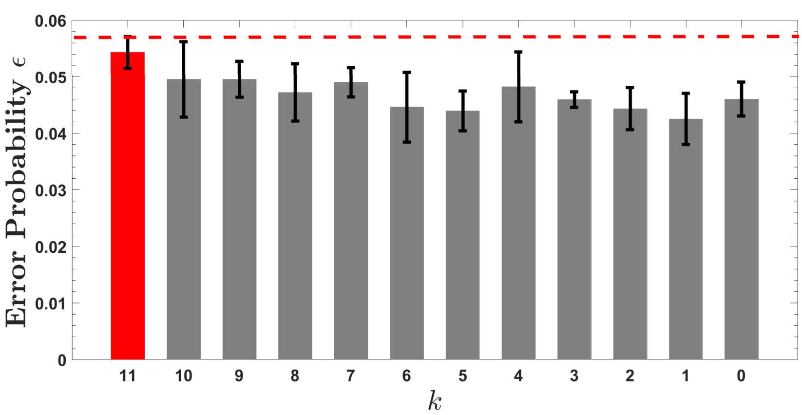
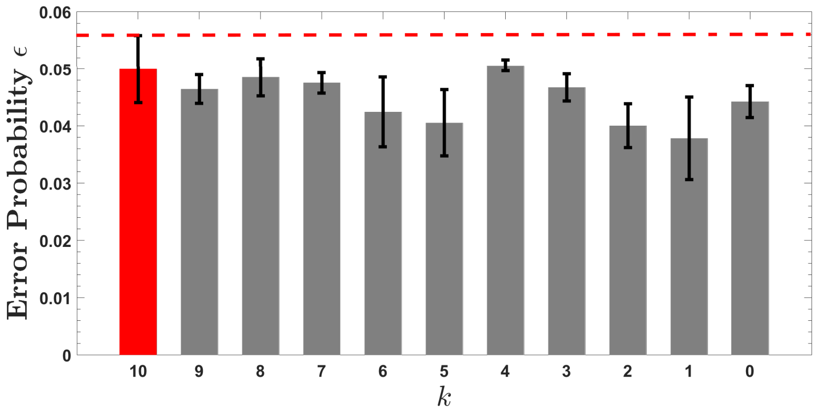
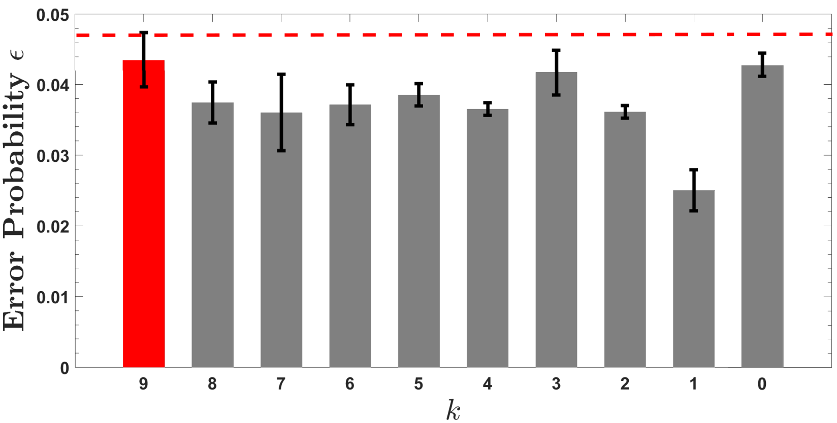
Table 2 shows the complete experimental results. Figure 8 shows the experimental error probabilities of different system sizes ranging from to 9. For each system size, the largest error probability is obtained in the worst case (red bar). The error bars represent 1 standard deviation. A possible reason why the error rises with growing system size is because the thermal expansion introduced by setting the different length of each section cannot be compensated, and results in a length mismatch as grows.
| System size () | 9 | 10 | 11 | 12 |
|---|---|---|---|---|
| Loss of Alice’s section (dB) | 1.340.04 | 1.390.04 | 1.780.04 | 2.060.04 |
| Loss of Bob’s section (dB) | 0.91.06 | 1.260.04 | 1.260.04 | 1.460.04 |
| System loss (dB) | ||||
| Error probability () | ||||
| Q | ||||
| (classical) | ||||
| (quantum definite) |
References
- Buhrman et al. (2010) H. Buhrman, R. Cleve, S. Massar, and R. de Wolf, Rev. Mod. Phys. 82, 665 (2010).
- Yao (1979) A. C.-C. Yao, in Proceedings of the 11th Annual ACM Symposium on Theory of Computing (ACM, New York, 1979), pp. 209–213.
- Brassard (2003) G. Brassard, Found. Phys. 33, 1593 (2003).
- Raz (1999) R. Raz, in Proceedings of the Thirty-First Annual ACM Symposium on Theory of Computing, STOC ’99 (ACM, New York, 1999) pp. 358–367.
- Buhrman et al. (2001) H. Buhrman, R. Cleve, J. Watrous, and R. de Wolf, Phys. Rev. Lett. 87, 167902 (2001).
- Bar-Yossef et al. (2004) Z. Bar-Yossef, T. S. Jayram, and I. Kerenidis, in Proceedings of the Thirty-sixth Annual ACM Symposium on Theory of Computing (ACM, New York, 2004), pp. 128–137.
- Gavinsky et al. (2007) D. Gavinsky, J. Kempe, I. Kerenidis, R. Raz, and R. de Wolf, in Proceedings of the Thirty-ninth Annual ACM Symposium on Theory of Computing, STOC ’07 (ACM, New York, 2007) pp. 516–525.
- Regev and Klartag (2011) O. Regev and B. Klartag, in Proceedings of the Forty-Third Annual ACM Symposium on Theory of Computing, STOC ’11 (ACM, New York, 2011), pp. 31–40.
- Arrazola and Lütkenhaus (2014) J. M. Arrazola and N. Lütkenhaus, Phys. Rev. A 89, 062305 (2014).
- Shor (1999) P. W. Shor, SIAM Rev. 41, 303 (1999).
- Horn et al. (2005) R. T. Horn, S. A. Babichev, K.-P. Marzlin, A. I. Lvovsky, and B. C. Sanders, Phys. Rev. Lett. 95, 150502 (2005).
- Xu et al. (2015) F. Xu, J. M. Arrazola, K. Wei, W. Wang, P. Palacios-Avila, C. Feng, S. Sajeed, N. Lütkenhaus, and H.-K. Lo, Nat. Commun. 6, 8735 (2015).
- Guan et al. (2016) J. Y. Guan, F. Xu, H. L. Yin, Y. Li, W. J. Zhang, S. J. Chen, X. Y. Yang, L. Li, L. X. You, T. Y. Chen, Z. Wang, Q. Zhang, and J. W. Pan, Phys. Rev. Lett. 116, 240502 (2016).
- Du et al. (2006) J. Du, P. Zou, X. Peng, D. K. L. Oi, L. C. Kwek, C. H. Oh, and A. Ekert, Phys. Rev. A 74, 042319 (2006).
- Trojek et al. (2005) P. Trojek, C. Schmid, M. Bourennane, Č. Brukner, M. Żukowski, and H. Weinfurter, Phys. Rev. A 72, 050305 (2005).
- Guérin et al. (2016) P. A. Guérin, A. Feix, M. Araújo, and Č. Brukner, Phys. Rev. Lett. 117, 100502 (2016).
- Oreshkov et al. (2012) O. Oreshkov, F. Costa, and Č. Brukner, Nat. Commun. 3, 1092 (2012).
- Chiribella et al. (2013) G. Chiribella, G. M. D’Ariano, P. Perinotti, and B. Valiron, Phys. Rev. A 88, 022318 (2013).
- Brukner (2014) Č. Brukner, Nat. Phys. 10, 259 (2014).
- Hardy (2007) L. Hardy, J. Phys. A 40, 3081 (2007).
- (21) M. Zych, F. Costa, I. Pikovski, and Č. Brukner, arXiv:1708.00248 .
- (22) G. Rubino, L. A. Rozema, F. Massa, M. Araújo, M. Zych, Č. Brukner, and P. Walther, arXiv:1712.06884 .
- Feix et al. (2015) A. Feix, M. Araújo, and Č. Brukner, Phys. Rev. A 92, 052326 (2015).
- Araújo et al. (2015) M. Araújo, C. Branciard, F. Costa, A. Feix, C. Giarmatzi, and Č. Brukner, New J. Phys. 17, 102001 (2015).
- Branciard et al. (2015) C. Branciard, M. Araújo, A. Feix, F. Costa, and Č. Brukner, New J. Phys. 18, 013008 (2015).
- Rubino et al. (2017) G. Rubino, L. A. Rozema, A. Feix, M. Araújo, J. M. Zeuner, L. M. Procopio, Č. Brukner, and P. Walther, Sci. Adv. 3, e1602589 (2017).
- Goswami et al. (2018) K. Goswami, C. Giarmatzi, M. Kewming, F. Costa, C. Branciard, J. Romero, and A. G. White, Phys. Rev. Lett. 121, 090503 (2018).
- Castro-Ruiz et al. (2018) E. Castro-Ruiz, F. Giacomini, and Č. Brukner, Phys. Rev. X 8, 011047 (2018).
- Araújo et al. (2017) M. Araújo, A. Feix, M. Navascués, and Č. Brukner, Quantum 1, 10 (2017).
- (30) O. Oreshkov, arXiv:1801.07594 .
- Araújo et al. (2014) M. Araújo, F. Costa, and Č. Brukner, Phys. Rev. Lett. 113, 250402 (2014).
- Procopio et al. (2015) L. M. Procopio, A. Moqanaki, M. Araujo, F. Costa, I. Alonso Calafell, E. G. Dowd, D. R. Hamel, L. A. Rozema, Č. Brukner, and P. Walther, Nat. Commun. 6, 7913 (2015).
- Ebler et al. (2018) D. Ebler, S. Salek, and G. Chiribella, Phys. Rev. Lett. 120, 120502 (2018).
- (34) K. Goswami, J. Romero, and A. G. White, arXiv:1807.07383 .
- Bartlett et al. (2002) S. D. Bartlett, H. de Guise, and B. C. Sanders, Phys. Rev. A 65, 052316 (2002).
- Patera and Zassenhaus (1988) J. Patera and H. Zassenhaus, J. Math. Phys. (N. Y.) 29, 665 (1988).
- Del Santo and Dakić (2018) F. Del Santo and B. Dakić, Phys. Rev. Lett. 120, 060503 (2018).
- (38) F. Massa, A. Moqanaki, F. Del Santo, B. Dakic, and P. Walther, arXiv:1802.05102 .
- U’Ren et al. (2005) A. B. U’Ren, C. Silberhorn, J. L. Ball, K. Banaszek, and I. A. Walmsley, Phys. Rev. A 72, 021802 (2005).
- Jin et al. (2015) R.-B. Jin, M. Fujiwara, T. Yamashita, S. Miki, H. Terai, Z. Wang, K. Wakui, R. Shimizu, and M. Sasaki, Opt. Commu. 336, 47 (2015).