跳到论文正文
W Papers独立论文阅读器 arXiv:1810.10086 论文正文 计算阅读时间 · 0%
引用这篇论文根据当前论文元数据生成,正式投稿前建议核对。


License: arXiv.org perpetual non-exclusive license
arXiv:1810.10086v1 [eess.SY] 16 Oct 2018

Finite-time Guarantees for Byzantine-Resilient Distributed State Estimation with Noisy Measurements

Lili Su    Shahin Shahrampour Thanks:  Thanks: Lili Su is with the Computer Science and Artificial Intelligence Laboratory, Massachusetts Institute of Technology, Cambridge, MA 02139 (lilisu@mit.edu). Thanks: Shahin Shahrampour is with the Department of Industrial and Systems Engineering, Texas A&M University, College Station, TX 77843 (shahin@tamu.edu).
Abstract

This work considers resilient, cooperative state estimation in unreliable multi-agent networks. A network of agents aims to collaboratively estimate the value of an unknown vector parameter, while an unknown subset of agents suffer Byzantine faults. Faulty agents malfunction arbitrarily and may send out highly unstructured messages to other agents in the network. As opposed to fault-free networks, reaching agreement in the presence of Byzantine faults is far from trivial. In this paper, we propose a computationally-efficient algorithm that is provably robust to Byzantine faults. At each iteration of the algorithm, a good agent (1) performs a gradient descent update based on noisy local measurements, (2) exchanges its update with other agents in its neighborhood, and (3) robustly aggregates the received messages using coordinate-wise trimmed means. Under mild technical assumptions, we establish that good agents learn the true parameter asymptotically in almost sure sense. We further complement our analysis by proving (high probability) finite-time convergence rate, encapsulating network characteristics.

I Introduction

Collaborative state/parameter estimation has attracted a considerable attention due to a wide range of applications in internet of things (IoT), wireless networks, power grids, sensor networks, and robotic networks [1, 2, 3, 4, 5, 6, 7]. In these applications, a network of (connected) agents collect information in a distributed fashion and share an overarching goal to learn the common unknown truth θ∗∈ℝd\theta^{*}\in{\mathbb{R}}^{d}. Local measurements obtained by each individual agent contain noisy and highly incomplete information about θ∗\theta^{*}. Nevertheless, the network of agents might be able to collaboratively learn θ∗\theta^{*} by effectively fusing the information contained in their local measurements.

In the absence of system adversary, the state estimation problem is well-studied [8, 5]. However, some practical scenarios such as IoT, micro-grids, and Federated Learning are vulnerable to faults [9]. Motivated by that, we are interested in addressing collaborative estimation in the presence of malicious agents. The existence of malicious agents might arise when some of the networked agents are compromised by a system adversary. Despite the wealth of literature on collaborative estimation with random link failures, packet-dropping failures, and crash failures (e.g. [10]), perhaps less well-known is estimation in the presence of highly unstructured failures or even adversarial agents, especially in finite-time domain.

In this work, to formally capture the unstructured system threat, we adopt Byzantine fault model [11] – a canonical fault model in distributed computing. In this model, there exists a system adversary that can choose up to a constant fraction of agents to compromise and control. An agent suffering Byzantine fault behaves arbitrarily badly by sending out unstructured malicious messages to the good agents. In addition, Byzantine agents may give conflicting messages to different agents in the system. Tolerating Byzantine faults is highly non-trivial (see e.g. [12, 13]). For example, it is well-known that in complete graphs, no algorithm can tolerate more than 1/31/3 of the agents to be Byzantine [13]. This difficulty arises partially from the system asymmetry caused by the conflicting messages sent by the Byzantine agents. In fact, Byzantine consensus with vector multi-dimensional inputs in the complete graphs had not been solved until only recently [14, 15].

Despite intensive efforts on securing distributed learning (see Section I-B for details), to the best of the authors’ knowledge, efficient algorithms that are provably resilient to Byzantine faults with less stringent assumptions on noisy local measurements are still lacking. In particular, the literature has mostly focused on the asymptotic analysis, leaving the finite-time guarantees for such algorithms a complementary direction to pursue, which is the main focal point of this work.

I-A Our Contributions

We propose a computationally-efficient algorithm that is provably robust to Byzantine faults. At each iteration of our algorithm, a good agent (1) performs a gradient descent update based on local measurements only, (2) exchanges its update with other agents in its neighborhood, and (3) robustly aggregates the received messages using coordinate-wise trimmed means.

For ease of exposition, we first present our results for fully connected networks (complete graphs), and then generalize the obtained results to general networks (incomplete graphs) assuming that the networks satisfy the necessary conditions such that Byzantine-resilient consensus with scalar inputs can be achievable. For both cases, we establish that every good agent learns the true parameter asymptotically in the almost sure sense. Most importantly, we characterize the finite-time convergence rate (in high-probability sense), encapsulating network characteristics. We finally provide numerical simulations for our method to verify our theoretical results.

I-B Related Literature

Resilient estimation, detection, and learning has attracted a great deal of attention in the past few years, and many researchers in the fields of control, signal processing, and network science have addressed the problem by adopting different notions of resilience or robustness.

In [16, 17, 18], resilience has been discussed in the context of smart power grid systems using cardinality minimization and its ℓ1\ell_{1} relaxations. On the other hand, the focus of [19, 20] is on estimation in Linear Time-Invariant (LTI) systems. In [19], an interesting approach is proposed for fault detection using monitors, and fundamental monitoring limitations have been characterized using tools from system theory and game theory. Furthermore, the approach of [20] is inspired from the areas of error-correction over the reals and compressed sensing. In [21], robust Kalman filtering is discussed, where the estimate updates are derived using a convex ℓ1\ell_{1} optimization problem. Authors of [22] consider a model where the observation noise is sparse, in the sense that the faulty sensors have noisy measurements, while other sensors measurements are noiseless. An event triggered projected gradient descent is then proposed to reconstruct the state. In our setting, though the state is fixed, we deal with multi-agent networks, i.e., the problem must be solved in a distributed manner since each agent has local (noisy) measurements from the state, and message passing schemes (e.g. consensus) are required to learn the state.

In parallel to advancements on resilient centralized estimation, recent years have witnessed intensive interest in securing distributed estimation. The authors of [23] discuss reaching consensus in the presence of malicious agents, assuming a broadcast model of communication. Chen et al. [24] propose a novel adversary detection strategy under which good agents either asymptotically learn the true state or detect the existence of a system fault. If a fault is flagged, the system goes through some external procedure to “repair” itself. As a result, the method does not perform estimation under system adversary (which is the focus of this paper). Furthermore, other resilient algorithms have been proposed [25, 26, 27, 28, 29] with different assumptions and performance guarantees. Chen et al. [25] propose an algorithm under which all of the agents’ estimates converge to the true state as long as less than one half of the agents are faulty. However, this algorithm works under the assumption that an agent can fully observe the true state in the non-faulty condition [25, Section II.A], as opposed to our model which deals with both observability and noisy measurement issues. Mitra and Sundaram [26] consider the more general LTI systems and characterize the fundamental limits on adversary-resilient algorithms. However, unlike our work, [26] deals with noiseless observations and the focus is on asymptotic analysis. Xu et al. [27] study the general dynamic optimization problem. They propose a total variation (TV) norm regularization technique to mitigate the effect of malfunctioning agents, but unfortunately, in the static case, the good agents cannot learn the true minimizer (see Corollary 1 in [27]). In fact, [27, Assumption 4] might not hold in the sense that under some strategies of the adversary agents, some good agents may appear to be bad to others, and the outgoing links from those agents might be cut off by the good agents. The lack of convergence in this case is consistent with the lower bound result in [30].

Another relevant work is the distributed hypothesis testing of [28] where the algorithm Byz-Iter is proposed. Though this algorithm may work for the state estimation problem, it scales poorly in dimension. Our algorithm is similar to [29] in that we both combine local gradient descent with coordinate-wise message trimming. Although [29] considers a more general optimization framework, it is implicitly assumed that the optimization problem can be separated into independent optimization problems (of the size of unknown parameter); otherwise, [29, Lemma 1] does not hold and the proof in [30] cannot be applied.

II Problem Formulation

II-A Network Model

We consider a multi-agent network which is a collection of nn agents/nodes communicating with each other through a communication network G⁡(𝒱,ℰ)G({\mathcal{V}},{\mathcal{E}}), where 𝒱={1,⋯,n}{\mathcal{V}}=\{1,\cdots,n\} and ℰ{\mathcal{E}} denote the set of nodes and edges, respectively. We denote by 𝒩i{\mathcal{N}}_{i} the set of incoming neighbors of agent ii. An unknown subset of agents of size at most bb, denoted by 𝒜{\mathcal{A}}, might be bad or adversarial. The set 𝒜{\mathcal{A}} is chosen by the system adversary. For ease of exposition, let

|𝒱/𝒜|=ϕ.|{\mathcal{V}}/{\mathcal{A}}|=\phi.

Clearly, ϕ≥n−b\phi\geq n-b.

Good agents (agents in 𝒱/𝒜{\mathcal{V}}/{\mathcal{A}}) aim to estimate the unknown parameter collaboratively, but bad agents (agents in 𝒜{\mathcal{A}}) can adversarially affect the estimation procedure by sending completely arbitrary, malicious, and possibly conflicting messages to the good agents.

II-B Observation Model

In this work, we focus on a linear observation model, where yi​(t)y_{i}(t) represents the local measurement of agent ii at time tt as follows

yi​(t)=Hi​θ∗+wi​(t),\displaystyle y_{i}(t)=H_{i}\theta^{*}+w_{i}(t), (1)

and Hi∈ℝni×dH_{i}\in{\mathbb{R}}^{n_{i}\times d} is the local observation matrix. The noise sequence wi​(t)w_{i}(t) is i.i.d.i.i.d. with 𝔼​[wi​(t)]=𝟎\mathbb{E}\left[w_{i}(t)\right]={\bf 0} and 𝔼⁡[wi​(t)​wi​(t)⊤]=Σi\mathbb{E}\left[w_{i}(t)w_{i}(t)^{\top}\right]=\Sigma_{i}. The sequences are bounded for all agents, i.e., there exists constant C>0C>0 such that ℙ{‖wi(t)‖2≤C}=1\mathbb{P}\left\{\left\|{w_{i}(t)}\right\|_{2}\leq C\right\}=1 for i∈𝒱i\in{\mathcal{V}}. Moreover, the noise sequences across good agents are independent. That is, (wi​(t),t≥1)\left(w_{i}(t),t\geq 1\right) and (wj​(t),t≥1)\left(w_{j}(t),t\geq 1\right) for i≠ji\not=j are independent. As in practice the observation matrix HiH_{i} is often fat, i.e., ni≪dn_{i}\ll d, each agent ii must obtain information from others to correctly estimate θ∗\theta^{*}.

II-C Fault Model

To formally capture the system threat, we adopt the Byzantine fault model [11] – a canonical fault model in distributed computing. In this model, there exists a system adversary that can choose up to bb of the nn agents (where b<nb<n) to compromise and control. Recall that this set of agents is denoted by 𝒜{\mathcal{A}}. An agent suffering Byzantine fault is referred to as Byzantine agent. While the set 𝒜{\mathcal{A}} is unknown to good agents, a standard assumption in the literature is that the value of bb is common knowledge [11].

The system adversary is extremely powerful in the sense that it has complete knowledge of the network, including the local program that each good agent is supposed to run, the true value of the parameter θ∗\theta^{*}, the current status and running history of the multi-agent network system, the running history, etc. Hence, the Byzantine agents can collude with each other and deviate from their pre-specified local programs to arbitrarily misrepresent information to the good agents. In particular, Byzantine agents can mislead each of the good agents in a unique fashion, i.e., letting mi​j​(t)∈ℝdm_{ij}(t)\in{\mathbb{R}}^{d} be the message sent from agent i∈𝒜i\in{\mathcal{A}} to agent j∈𝒱∖𝒜j\in{\mathcal{V}}\setminus{\mathcal{A}} at time tt, it is possible that mi​j​(t)≠mi​j′​(t)m_{ij}(t)\not=m_{i{j^{\prime}}}(t) for j≠j′∈𝒱∖𝒜j\not=j^{\prime}\in{\mathcal{V}}\setminus{\mathcal{A}}.

Remark 1.

Note that due to the extreme freedom given to Byzantine agents and the system asymmetry caused by them, a resilient distributed solution to the estimation problem is highly non-trivial even in complete graphs. In particular, it is well-known that in complete graphs, no algorithm can tolerate more than 1/31/3 of the agents to be Byzantine [13].

II-D Finite-time vs. Asymptotic Local Functions

The Byzantine-resilient state estimation problem can be viewed with an optimization lens, where each good agent would only asymptotically know its local function. For each agent i∈𝒱i\in{\mathcal{V}}, define the asymptotic local function fi:ℝd→ℝf_{i}:{\mathbb{R}}^{d}\to{\mathbb{R}} as

fi​(x)\displaystyle f_{i}(x) ≜𝔼⁡[12​‖Hi​x−yi‖22],\displaystyle\triangleq\mathbb{E}\left[\frac{1}{2}\left\|{H_{i}x-y_{i}}\right\|_{2}^{2}\right], (2)

where the expectation is taken over the randomness of wiw_{i}. Note that fif_{i} is well-defined for each i∈𝒱i\in{\mathcal{V}} regardless of whether it is suffering Byzantine faults or not. Since the distribution of wiw_{i} is unknown to agent ii, at any finite tt, function fif_{i} is not accessible to agent ii. However, the agent has access to the finite-time or empirical local function

fi,t​(x)≜1t​∑s=1t12​‖Hi​x−yi​(s)‖22,\displaystyle f_{i,t}(x)\triangleq\frac{1}{t}\sum_{s=1}^{t}\frac{1}{2}\left\|{H_{i}x-y_{i}(s)}\right\|_{2}^{2}, (3)

whose gradient at xx is

∇fi,t​(x)\displaystyle\nabla f_{i,t}(x) =Hi⊤​Hi​(x−θ∗)−Hi⊤​1t​∑r=1twi​(t).\displaystyle=H_{i}^{\top}H_{i}\left(x-\theta^{*}\right)-H_{i}^{\top}\frac{1}{t}\sum_{r=1}^{t}w_{i}(t). (4)

III Byzantine-Resilient State Estimation

To robustify distributed state estimation against Byzantine faults, one approach may be to combine the local gradient descent with multi-dimensional Byzantine-resilient consensus [28, 15, 14] (which typically relies on using Tverberg points). However, the performance of any such algorithm is proved to scale poorly in the dimension of the parameter dd [28, 15, 14]. This is partially due to the fact that different dimensions of the inputs strongly interfere with each other, and the Byzantine agents can inject wrong information with both extreme magnitudes and directions.

To improve the scalability with respect to dd and to improve the computation complexity, instead of multi-dimensional Byzantine-resilient consensus, we robustly aggregate the received messages using coordinate-wise trimmed means.

III-A Algorithm

We propose an algorithm, named Byzantine-resilient state estimation, where each good agent iteratively aggregates the received messages. To robustify, the agent discards the largest bb and the smallest bb values for each component. In particular, in each iteration, an agent performs the following three steps:

  • •

    Local gradient descent: Agent ii first computes the noisy local gradient ∇fi,t​(xi​(t−1))\nabla f_{i,t}(x_{i}(t-1)), and performs local gradient descent to obtain zi​(t)z_{i}(t), i.e.,

    zi​(t)=xi​(t−1)−∇fi,t​(xi​(t−1)).\displaystyle z_{i}(t)=x_{i}(t-1)-\nabla f_{i,t}(x_{i}(t-1)).

    Note that the step-size used in this update is 1.

  • •

    Information exchange: It exchanges zi​(t)z_{i}(t) with other agents in its local neighborhood. Recall that mi​j​(t)∈ℝdm_{ij}(t)\in{\mathbb{R}}^{d} is the message sent from agent ii to agent jj at time tt. It relates to zi​(t)z_{i}(t) as follows:

    mi​j​(t)={zi​(t)if​i∈(𝒱/𝒜);⋆if​i∈𝒜,\displaystyle m_{ij}(t)=\begin{cases}z_{i}(t)&~~~\text{if}~i\in({\mathcal{V}}/{\mathcal{A}});\\ \star&~~~\text{if}~i\in{\mathcal{A}},\end{cases}

    where ⋆\star denotes an arbitrary value. Byzantine agents can mislead good agents differently, i.e., if i∈𝒜i\in{\mathcal{A}}, it might hold that mi​j​(t)≠mi​j′​(t)m_{ij}(t)\not=m_{i{j^{\prime}}}(t) for j≠j′∈𝒱∖𝒜j\not=j^{\prime}\in{\mathcal{V}}\setminus{\mathcal{A}}.

  • •

    Robust aggregation: For each component k=1,…,dk=1,\ldots,d, the agent computes the trimmed mean and uses them to obtain xi​(t)x_{i}(t).

The formal description of the algorithm for agent i∈𝒱∖𝒜i\in{\mathcal{V}}\setminus{\mathcal{A}} is given in Algorithm 1.

Input: bb and TT
Initialization: Set xi​(0)x_{i}(0) to an arbitrary value for each agent i∈𝒱i\in{\mathcal{V}}
for t=1,…,Tt=1,\ldots,T do
   - Obtain a new measurement yi​(t)y_{i}(t);
   
   - Compute the local noisy gradient ∇fi,t​(xi​(t−1))\nabla f_{i,t}(x_{i}(t-1)) according to (4);
   
   - Compute zi​(t)=xi​(t−1)−∇fi,t​(xi​(t−1))z_{i}(t)=x_{i}(t-1)-\nabla f_{i,t}(x_{i}(t-1));
   
   - Send zi​(t)z_{i}(t) to its outgoing neighbors;
   
   for k=1,…,dk=1,\ldots,d do
   
      - Sort the kk–th component of the received messages mj​i​(t)m_{ji}(t) for j∈𝒩i∪{i}j\in{\mathcal{N}}_{i}\cup\{i\} in a non-decreasing (increasing) order;
       - Remove the largest bb values and the smallest bb values;
      
      - Denote the remained “agent” indices set as ℛik​(t){\mathcal{R}}_{i}^{k}(t) and set
xik​(t)=1|ℛik​(t)|​∑j∈ℛik​(t)⟨mj​i​(t),ek⟩.x_{i}^{k}(t)=\frac{1}{\left|{\mathcal{R}}_{i}^{k}(t)\right|}\sum_{j\in{\mathcal{R}}_{i}^{k}(t)}\left\langle m_{ji}(t),e_{k}\right\rangle.
end for
   - Set (xi​(t))⊤=(xi1​(t),…,xid​(t))(x_{i}(t))^{\top}=\left(x_{i}^{1}(t),\ldots,x_{i}^{d}(t)\right). end for
Output: xi​(T)x_{i}(T).
Algorithm 1 Byzantine-resilient state estimation

IV Finite-time Guarantee for Complete Networks

In this section, we provide results for the case that G⁡(𝒱,ℰ)G({\mathcal{V}},{\mathcal{E}}) is a complete graph. Beside the fact that the technical analysis of complete graphs would be different from that of incomplete graphs (in terms of assumptions), the former is particularity interesting in computer networks. In fact, in many computer networks efficient communication protocols (such as TCP/IP) can be implemented such that any two computer are logically connected.

It can be shown that the update of xix_{i} uses the information provided by the good agents only. In addition, each of the good agent has limited impact on xix_{i}, formally stated next.

Lemma 1.

For each iteration tt, each good agent i∈𝒱/𝒜i\in{\mathcal{V}}/{\mathcal{A}}, and each kk, there exist coefficients (βi​jk​(t),j∈𝒱/𝒜)\left(\beta_{ij}^{k}(t),~j\in{\mathcal{V}}/{\mathcal{A}}\right) such that

  • •

    xik​(t)=∑j∈𝒱/𝒜βi​jk​(t)​⟨zj​(t),ek⟩x_{i}^{k}(t)=\sum_{j\in{\mathcal{V}}/{\mathcal{A}}}\beta_{ij}^{k}(t)\left\langle z_{j}(t),e_{k}\right\rangle;

  • •

    0≤βi​jk​(t)≤1ϕ−b0\leq\beta_{ij}^{k}(t)\leq\frac{1}{\phi-b} for all j∈𝒱/𝒜j\in{\mathcal{V}}/{\mathcal{A}} and ∑j∈𝒱/𝒜βi​jk​(t)=1\sum_{j\in{\mathcal{V}}/{\mathcal{A}}}\beta_{ij}^{k}(t)=1.

Notice that the sets of convex coefficients for different values of kk might be different, i.e., (βi​jk​(t),j∈𝒱/𝒜)≠(βi​jk′​(t),j∈𝒱/𝒜)\left(\beta_{ij}^{k}(t),~j\in{\mathcal{V}}/{\mathcal{A}}\right)\not=\left(\beta_{ij}^{k^{\prime}}(t),~j\in{\mathcal{V}}/{\mathcal{A}}\right) for k≠k′k\not=k^{\prime}. Moreover, even for the same kk, the convex coefficients might be different for different good agents, i.e., (βi​jk​(t),j∈𝒱/𝒜)≠(βi′​jk​(t),j∈𝒱/𝒜)\left(\beta_{ij}^{k}(t),~j\in{\mathcal{V}}/{\mathcal{A}}\right)\not=\left(\beta_{i^{\prime}j}^{k}(t),~j\in{\mathcal{V}}/{\mathcal{A}}\right) for i≠i′i\not=i^{\prime}. This stems from the freedom of Byzantine agents in sending different messages across agents, i.e., ma​j≠ma​j′m_{aj}\not=m_{aj^{\prime}} if a∈𝒜a\in{\mathcal{A}} and j≠j′j\not=j^{\prime}.

To prove the convergence of Algorithm 1, we use the following assumption.

Assumption 1.

For all k=1,⋯,dk=1,\cdots,d, we have that

1ϕ−b​∑j∈𝒱/𝒜‖(𝐈−Hj⊤​Hj)​ek‖1<1.\displaystyle\frac{1}{\phi-b}\sum_{j\in{\mathcal{V}}/{\mathcal{A}}}\left\|{\left({\bf I}-H_{j}^{\top}H_{j}\right)e_{k}}\right\|_{1}<1.

Note that ‖(𝐈−Hj⊤​Hj)​ek‖1\left\|{\left({\bf I}-H_{j}^{\top}H_{j}\right)e_{k}}\right\|_{1} is the ℓ1\ell_{1} norm of the kk–th column of matrix 𝐈−Hj⊤​Hj{\bf I}-H_{j}^{\top}H_{j}. It can well be the case that ‖(𝐈−Hj⊤​Hj)​ek‖1≥1\left\|{\left({\bf I}-H_{j}^{\top}H_{j}\right)e_{k}}\right\|_{1}\geq 1 for some good agents. However, Assumption 1 implies that for each k=1,⋯,dk=1,\cdots,d, there exists at least b+1b+1 good agents such that

‖(𝐈−Hj⊤​Hj)​ek‖1<1.\displaystyle\left\|{\left({\bf I}-H_{j}^{\top}H_{j}\right)e_{k}}\right\|_{1}<1.

The above assumption is imposed for the dd components individually. None of the agents are required to satisfy ‖(𝐈−Hj⊤​Hj)​ek‖1<1\left\|{\left({\bf I}-H_{j}^{\top}H_{j}\right)e_{k}}\right\|_{1}<1 simultaneously for all k=1,⋯,dk=1,\cdots,d. Now, let

ρ≜maxk:1≤k≤d∑j∈𝒱/𝒜‖(𝐈−Hj⊤​Hj)​ek‖1ϕ−b.\displaystyle\rho~\triangleq~\max_{k:1\leq k\leq d}\frac{\sum_{j\in{\mathcal{V}}/{\mathcal{A}}}\left\|{\left({\bf I}-H_{j}^{\top}H_{j}\right)e_{k}}\right\|_{1}}{\phi-b}. (5)

Clearly, ρ<1\rho<1 under Assumption 1. For ease of exposition, for each j∈𝒱/𝒜j\in{\mathcal{V}}/{\mathcal{A}} and for any λ∈(0,1)\lambda\in(0,1), let

Rj​(λ,t)≜∑m=0t−1λm​‖∑r=1t−mwj​(r)t−m‖2.\displaystyle R_{j}(\lambda,t)~\triangleq~\sum_{m=0}^{t-1}\lambda^{m}\left\|{\frac{\sum_{r=1}^{t-m}w_{j}(r)}{t-m}}\right\|_{2}. (6)

The following two concentration results are two key auxiliary lemmas for our main theorem.

Lemma 2.

Suppose Assumption 1 holds. Then, for each j∈𝒱/𝒜j\in{\mathcal{V}}/{\mathcal{A}} and for any λ∈(0,1)\lambda\in(0,1)

limt→∞Rj​(λ,t)=0​almost surely.\displaystyle\lim_{t\to\infty}R_{j}(\lambda,t)~=~0~~\text{almost surely}.

In addition, we characterize the finite-time convergence rate of Rj​(λ,⋅)R_{j}(\lambda,\cdot) for any fixed λ\lambda.

Lemma 3.

Suppose Assumption 1 holds. Then for each j∈𝒱/𝒜j\in{\mathcal{V}}/{\mathcal{A}} and for any λ∈(0,1)\lambda\in(0,1)

ℙ{Rj(λ,t)≥𝗍𝗋𝖺𝖼𝖾⁡(Σj)∑m=1t−1λm1t−m+ϵ}\displaystyle\mathbb{P}\left\{R_{j}(\lambda,t)\geq\sqrt{\mathsf{trace}(\Sigma_{j})}\sum_{m=1}^{t-1}\lambda^{m}\frac{1}{\sqrt{t-m}}+\epsilon\right\}
≤exp⁡(−ϵ2​(1−λ)2​t8​C2),\displaystyle\leq\exp\left(\frac{-\epsilon^{2}(1-\lambda)^{2}t}{8C^{2}}\right),

Lemma 3 implies that ∀j∈𝒱/𝒜\forall j\in{\mathcal{V}}/{\mathcal{A}}, with probability at least 1−δ1-\delta, Rj​(t)=O​((log⁡1δ)/t)R_{j}(t)=O\left(\sqrt{\left(\log\frac{1}{\delta}\right)/t}\right).

Theorem 1.

Suppose Assumption 1 holds and the graph G⁡(𝒱,ℰ)G({\mathcal{V}},{\mathcal{E}}) is complete. Then

maxi∈𝒱/𝒜⁡‖xi​(t)−θ∗‖∞→a.s.0.\max_{i\in{\mathcal{V}}/{\mathcal{A}}}\left\|{x_{i}(t)-\theta^{*}}\right\|_{\infty}\xrightarrow{{\rm a.s.}}0.

Moreover, with probability at least
1−ϕ​exp⁡(−ϵ2​(1−ρ)2​t8​C2)1-\phi\exp\left(\frac{-\epsilon^{2}(1-\rho)^{2}t}{8C^{2}}\right), it holds that

maxi∈𝒱/𝒜⁡‖xi​(t)−θ∗‖∞≤ρt​maxi∈𝒱/𝒜​‖xi​(0)−θ∗‖∞\displaystyle\max_{i\in{\mathcal{V}}/{\mathcal{A}}}\left\|{x_{i}(t)-\theta^{*}}\right\|_{\infty}\leq\rho^{t}\max_{i\in{\mathcal{V}}/{\mathcal{A}}}\left\|{x_{i}(0)-\theta^{*}}\right\|_{\infty}
+C0(∑i∈𝒱/𝒜𝗍𝗋𝖺𝖼𝖾⁡(Σj))∑m=1t−1ρmt−m+ϕϵ,\displaystyle\quad+C_{0}\left(\sum_{i\in{\mathcal{V}}/{\mathcal{A}}}\sqrt{\mathsf{trace}(\Sigma_{j})}\right)\sum_{m=1}^{t-1}\frac{\rho^{m}}{\sqrt{t-m}}+\phi\epsilon,

where C0≜maxi∈𝒱/𝒜⁡‖Hi‖2C_{0}~\triangleq~\max_{i\in{\mathcal{V}}/{\mathcal{A}}}\left\|H_{i}\right\|_{2}.

The theorem indicates that all good agents (in a complete graph) are eventually able to learn the true parameter θ∗\theta^{*} almost surely. Also, with high probability the rate can be characterized as above, providing a finite-time guarantee for resilient estimation. The finite-time bound captures the performance, in terms of Σj\Sigma_{j}, the noise covariance for agent j∈𝒱/𝒜j\in{\mathcal{V}}/{\mathcal{A}}, as well as ρ\rho, which can crudely serve as a measure of observability in view of (5).

V Finite-time Guarantees for Incomplete Networks

V-A Incomplete Graphs: Multihop Communication

So far, our analysis of Algorithm 1 has focused on complete graphs.

For computer networks, this is a reasonable assumption as computers are connected to each other through some communication (routing) protocols. Our results are also applicable to wireless networks under some implementation assumptions.

Concretely, let G⁡(𝒱,ℰ)G({\mathcal{V}},{\mathcal{E}}) be the physical network that is not fully connected. Suppose the networked agents are allowed to relay the messages sent by others such that multi-hop communication can be implemented. We can adopt coding to force the Byzantine agents to either refuse to relay information or faithfully relay the messages without alternation [12]. Thus, as long as the node-connectively of G⁡(𝒱,ℰ)G({\mathcal{V}},{\mathcal{E}}) is at least b+1b+1, each good agent can reliably receive messages from other good agents in the network. We can use our algorithm to robust aggregate the received messages and perform one-step update. Similar analysis applies.

V-B Incomplete Graphs: Local Communication

Message forwarding might be costly or even infeasible for some wireless networks. Algorithms that rely solely on local communication are still highly desirable. Fortunately, with reasonable assumptions, Algorithm 1 works. Our algorithm is a consensus-based algorithm, so to make the paper self-contained, we briefly review relevant existing results on Byzantine consensus.

V-B1 Byzantine Consensus with Scalar Inputs

Note that, in contrast to fault-free consensus, Byzantine-resilient consensus with scalar inputs and with multidimensional inputs are fundamentally different [14, 15, 31]. Our algorithm relies on Byzantine-resilient consensus with scalar inputs.

Tight topological conditions are characterized in [31], where the conditions are stated in terms of a family of subgraphs of G⁡(𝒱,ℰ)G({\mathcal{V}},{\mathcal{E}}). Those subgraphs capture the “real” information flow under the message trimming strategy. Informally speaking, trimming certain messages can be viewed as ignoring (or removing) incoming links that carry the outliers. The non-uniqueness of the subgraph arises partially from the fact that the Byzantine agents can behave adaptively and arbitrarily. Such subgraphs are referred to as reduced graphs, defined as follows.

Definition 1.

[31] A reduced graph HH of G⁡(𝒱,ℰ)G({\mathcal{V}},{\mathcal{E}}) is obtained by (i) removing all faulty nodes 𝒜{\mathcal{A}}, and all the links incident on the faulty nodes 𝒜{\mathcal{A}}; and (ii) for each non-faulty node (nodes in 𝒱/𝒜{\mathcal{V}}/{\mathcal{A}}), removing up to bb additional incoming links.

It is important to note that the non-faulty agents do not know the identities of the faulty agents. Let ℋ{\mathcal{H}} be the collection of all reduced graphs of G⁡(𝒱,ℰ)G({\mathcal{V}},{\mathcal{E}}), and let

ξ:=|ℋ|.\xi:=\left|{\mathcal{H}}\right|.
Definition 2.

A source component in a given reduced graph is a strongly connected component, which does not have any incoming links from outside of that component.

It turns out that the effective communication network is potentially time-varying (partly) due to time-varying behaviors of Byzantine agents. The tight network topology condition for scaler valued consensus to be achievable is characterized in [31].

Theorem 2.

[31] For scalar inputs, iterative approximate Byzantine consensus is achievable among non-faulty agents if and only if every reduced graph of G⁡(𝒱,ℰ)G({\mathcal{V}},{\mathcal{E}}) contains only one source component.

Under the condition in Theorem 2, it follows that in any reduced graph, a node in the source component can reach every other nodes.

V-B2 Correctness of Algorithm 1 for Incomplete Graphs

We will show the correctness of our Algorithm 1 assuming that Byzantine consensus with scalar inputs is achievable over G⁡(𝒱,ℰ)G({\mathcal{V}},{\mathcal{E}}), and the following assumption holds.

Assumption 2.

For each non-faulty node j∈𝒱/𝒜j\in{\mathcal{V}}/{\mathcal{A}} and each k=1,⋯,dk=1,\cdots,d,

‖(𝐈−Hj⊤​Hj)​ek‖1≤1.\displaystyle\left\|{\left({\bf I}-H_{j}^{\top}H_{j}\right)e_{k}}\right\|_{1}~\leq~1.

In addition, any reduced graph HH contains a node in its unique source component such that for all k=1,⋯,dk=1,\cdots,d,

|(𝒩i∪{i}/𝒜)∩{j:‖(𝐈−Hj⊤​Hj)​ek‖1<1}|≥b+1.\displaystyle\left|({\mathcal{N}}_{i}\cup\{i\}/{\mathcal{A}})\cap\left\{j:\left\|{\left({\bf I}-H_{j}^{\top}H_{j}\right)e_{k}}\right\|_{1}<1\right\}\right|\geq b+1.

Note that in Assumption 2, 𝒩i{\mathcal{N}}_{i} is the incoming neighbors of node ii in the original graph G⁡(𝒱,ℰ)G({\mathcal{V}},{\mathcal{E}}).

Define ρ0\rho_{0} as

ρ0:=max1≤k≤dmaxj:‖(𝐈−Hj⊤​Hj)​ek‖1<1‖(𝐈−Hj⊤Hj)ek‖1.\displaystyle\rho_{0}:=\max_{1\leq k\leq d}\max_{j:\left\|{\left({\bf I}-H_{j}^{\top}H_{j}\right)e_{k}}\right\|_{1}<1}\left\|{\left({\bf I}-H_{j}^{\top}H_{j}\right)e_{k}}\right\|_{1}. (7)

In (7), the maximization

maxj:‖(𝐈−Hj⊤​Hj)​ek‖1<1‖(𝐈−Hj⊤Hj)ek‖1\max_{j:\left\|{\left({\bf I}-H_{j}^{\top}H_{j}\right)e_{k}}\right\|_{1}<1}\left\|{\left({\bf I}-H_{j}^{\top}H_{j}\right)e_{k}}\right\|_{1}

is taken over the non-faulty nodes only.

Similar to the analysis for the complete graphs, it can be shown that the update of xix_{i} uses the information provided by its good neighbors only.

Lemma 4.

[32, Claim 2] For each iteration tt, each good agent i∈𝒱/𝒜i\in{\mathcal{V}}/{\mathcal{A}}, and each kk, there exist coefficients (βi​jk​(t),j∈𝒩i∪{i})\left(\beta_{ij}^{k}(t),~j\in{\mathcal{N}}_{i}\cup\{i\}\right) such that

  • •

    xik​(t)=∑j∈𝒩i∪{i}/𝒜βi​jk​(t)​⟨zj​(t),ek⟩x_{i}^{k}(t)=\sum_{j\in{\mathcal{N}}_{i}\cup\{i\}/{\mathcal{A}}}\beta_{ij}^{k}(t)\left\langle z_{j}(t),e_{k}\right\rangle;

  • •

    There exists a subset of ℬi​(t)⊆𝒩i∪{i}/𝒜{\mathcal{B}}_{i}(t)\subseteq{\mathcal{N}}_{i}\cup\{i\}/{\mathcal{A}} such that |ℬ⁡(t)|≥|𝒩i∪{i}/𝒜|−b|{\mathcal{B}}(t)|\geq|{\mathcal{N}}_{i}\cup\{i\}/{\mathcal{A}}|-b and βi​jk​(t)≥12​(|𝒩i∪{i}/𝒜|−b)\beta_{ij}^{k}(t)\geq\frac{1}{2(|{\mathcal{N}}_{i}\cup\{i\}/{\mathcal{A}}|-b)} for each j∈ℬi​(t)j\in{\mathcal{B}}_{i}(t).

In the next theorem, we establish that (under the assumption above) the estimates of all agents are consistent almost surely, and furthermore, we characterize the (high probability) finite-time convergence rate of these estimates.

Theorem 3.

Suppose that every reduced graph of G⁡(𝒱,ℰ)G({\mathcal{V}},{\mathcal{E}}) contains a single source component, and Assumption 2 holds. Then

maxi∈𝒱/𝒜⁡‖xi​(t)−θ∗‖∞→a.s.0.\max_{i\in{\mathcal{V}}/{\mathcal{A}}}\left\|{x_{i}(t)-\theta^{*}}\right\|_{\infty}\xrightarrow{{\rm a.s.}}0.

Let γ:=1−1−ρ0(2​(ϕ−b))ξ​ϕ\gamma:=1-\frac{1-\rho_{0}}{\left(2(\phi-b)\right)^{\xi\phi}}. With probability at least
1−ϕ​exp⁡(−ϵ2​(1−γ1ξ​ϕ)2​t8​C2)1-\phi\exp\left(\frac{-\epsilon^{2}(1-\gamma^{\frac{1}{\xi\phi}})^{2}t}{8C^{2}}\right), it holds that

maxi∈𝒱/𝒜⁡‖xi​(t)−θ∗‖∞≤γtξ​ϕ​maxi∈𝒱/𝒜​‖xi​(0)−θ∗‖∞\displaystyle\max_{i\in{\mathcal{V}}/{\mathcal{A}}}\left\|{x_{i}(t)-\theta^{*}}\right\|_{\infty}\leq\gamma^{\frac{t}{\xi\phi}}\max_{i\in{\mathcal{V}}/{\mathcal{A}}}\left\|{x_{i}(0)-\theta^{*}}\right\|_{\infty}
+C0(∑i∈𝒱/𝒜𝗍𝗋𝖺𝖼𝖾⁡(Σj))∑m=1t−1γmξ​ϕt−m+ϕϵ.\displaystyle\quad+C_{0}\left(\sum_{i\in{\mathcal{V}}/{\mathcal{A}}}\sqrt{\mathsf{trace}(\Sigma_{j})}\right)\sum_{m=1}^{t-1}\frac{\gamma^{\frac{m}{\xi\phi}}}{\sqrt{t-m}}+\phi\epsilon.

VI Numerical Experiments

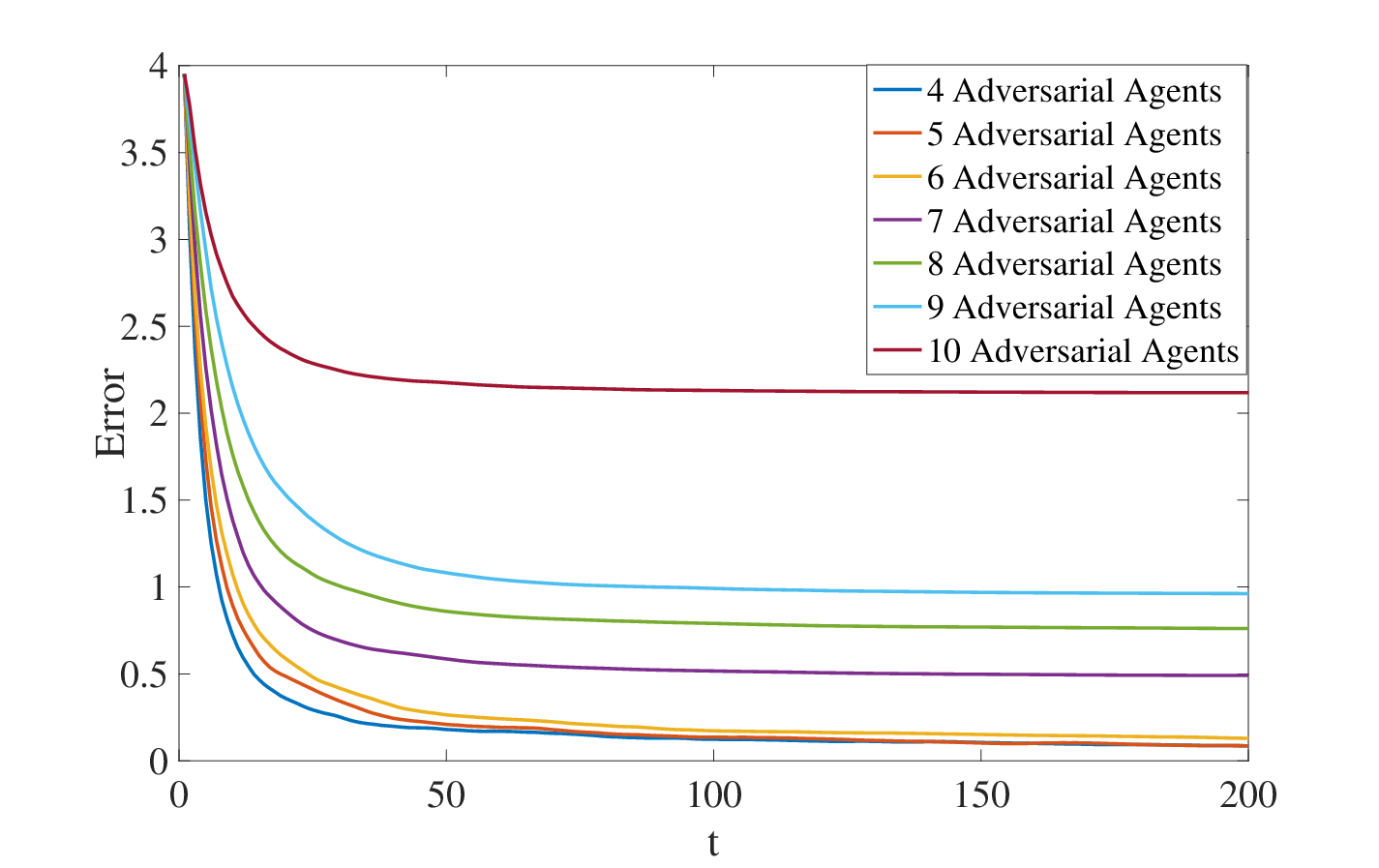
We now provide empirical evidence in support of our algorithm. We consider a complete graph of |𝒱∖𝒜|=30|{\mathcal{V}}\setminus{\mathcal{A}}|=30 agents. Each component of the unknown parameter θ∗∈ℝ50\theta^{*}\in{\mathbb{R}}^{50} is generated randomly within the interval [−1,1][-1,1] and is fixed thereafter during the estimation process. Moreover, the observation matrices Hi∈ℝ20×50H_{i}\in{\mathbb{R}}^{20\times 50} for each ii are chosen such that Assumption 1 holds.

Evidently, in this example, ni=20n_{i}=20 for all ii. Throughout, the adversarial agents can send out completely arbitrary messages in lieu of true gradients. We generate these arbitrary messages using a random 5050-dimensional vector, each component of which is sampled from 𝒩⁡(0,9){\mathcal{N}}(0,9).

Let us now define the network performance metric as

Error​(t)≜1ϕ​∑i∈𝒱∖𝒜‖θ∗−xi​(t)‖\text{Error}(t)\triangleq\frac{1}{\phi}\sum_{i\in{\mathcal{V}}\setminus{\mathcal{A}}}\|\theta^{*}-x_{i}(t)\|

and plot in Fig. 1 the error for various values of adversarial agents |𝒜|∈{4,5,…,10}|{\mathcal{A}}|\in\{4,5,\ldots,10\}. We observe a dichotomy, where for |𝒜|<7|{\mathcal{A}}|<7 the error converges to zero, whereas for |𝒜|≥7|{\mathcal{A}}|\geq 7 the convergence does not occur. Moreover, increase in the number of adversarial agents degrades the performance.

Refer to caption
Fig. 1: The plot of error decay versus time for different number of adversarial agents.

VII Conclusion

We studied resilient distributed estimation, where a network of agents want to learn the value of an unknown parameter in the presence of Byzantine agents. The main challenges in the problem are as follows: (i) Byzantine agents send out arbitrary messages to other agents, (ii) good agents need to deal with noisy measurements, and (iii) the parameter is not locally observable. We proposed an algorithm that allows agents to collectively learn the true parameter asymptotically in almost sure sense, and we further complemented our results with finite-time analysis. Future directions include resilient estimation and learning in a more general setting, where agents observations can be a nonlinear function of the unknown parameter. Another interesting direction is to investigate the minimal condition needed on the local observation matrices of the good agents for the problem to be solvable.

Proof of Lemma 1

We prove this lemma by construction. Note that this construction is only used in the algorithm analysis rather than an algorithm input. That is, to run the algorithm, each agent (either good or faulty) does not need to know β\beta.

For ease of exposition, let [ℛik​(t)]+[{\mathcal{R}}_{i}^{k}(t)]^{+} and [ℛik​(t)]−[{\mathcal{R}}_{i}^{k}(t)]^{-} be the non-overlapping subsets of 𝒱{\mathcal{V}} whose gradient’s kk–th entry are trimmed away by agent ii. Precisely,
(a) |[ℛik​(t)]−|=b=|[ℛik​(t)]+|\left|[{\mathcal{R}}_{i}^{k}(t)]^{-}\right|=b=\left|[{\mathcal{R}}_{i}^{k}(t)]^{+}\right|;
(b) [ℛik​(t)]−[{\mathcal{R}}_{i}^{k}(t)]^{-}, [ℛik​(t)]+[{\mathcal{R}}_{i}^{k}(t)]^{+} and ℛik​(t){\mathcal{R}}_{i}^{k}(t) partition set 𝒱{\mathcal{V}};
(c) ∀\forall j′∈[ℛik​(t)]−,j∈ℛik​(t),and ​j′′∈[ℛik​(t)]+j^{\prime}\in[{\mathcal{R}}_{i}^{k}(t)]^{-},j\in{\mathcal{R}}_{i}^{k}(t),~\text{and }j^{\prime\prime}\in[{\mathcal{R}}_{i}^{k}(t)]^{+} it holds that

⟨mj′​i​(t),ek⟩≤⟨mj​i​(t),ek⟩≤⟨mj′′​i​(t),ek⟩.\displaystyle\left\langle m_{j^{\prime}i}(t),e_{k}\right\rangle\leq\left\langle m_{ji}(t),e_{k}\right\rangle\leq\left\langle m_{j^{\prime\prime}i}(t),e_{k}\right\rangle. (8)

We consider two cases: (1) ℛik​(t)∩𝒜=∅{\mathcal{R}}_{i}^{k}(t)\cap{\mathcal{A}}=\emptyset; and (2) ℛik​(t)∩𝒜≠∅{\mathcal{R}}_{i}^{k}(t)\cap{\mathcal{A}}\not=\emptyset.

Case 1: Suppose that ℛik​(t)∩𝒜=∅{\mathcal{R}}_{i}^{k}(t)\cap{\mathcal{A}}=\emptyset. We construct the convex coefficients as follows:

Case 1-1: When |𝒜|=b\left|{\mathcal{A}}\right|=b, we have ϕ−b=n−2​b.\phi-b=n-2b. We choose the convex coefficients as

βi​jk​(t)={1n−2​b,∀j∈ℛik​(t),and0,∀j∉ℛik​(t).\displaystyle\beta_{ij}^{k}(t)=\begin{cases}&\frac{1}{n-2b},~~\forall j\in{\mathcal{R}}_{i}^{k}(t),\text{and}\\ &0,~~\forall j\notin{\mathcal{R}}_{i}^{k}(t).\end{cases}

Clearly, in this construction, βi​jk​(t)≤1ϕ−b\beta_{ij}^{k}(t)\leq\frac{1}{\phi-b}.

Case 1-2: When |𝒜|<b\left|{\mathcal{A}}\right|<b, it holds that

|[ℛik​(t)]−/𝒜|≥b−|𝒜|,\displaystyle\left|[{\mathcal{R}}_{i}^{k}(t)]^{-}/{\mathcal{A}}\right|\geq b-|{\mathcal{A}}|, (9)

and

|[ℛik​(t)]+/𝒜|≥b−|𝒜|.\displaystyle\left|[{\mathcal{R}}_{i}^{k}(t)]^{+}/{\mathcal{A}}\right|\geq b-|{\mathcal{A}}|. (10)

By (8), we have

1|[ℛik​(t)]−/𝒜|​∑j∈[ℛik​(t)]−/𝒜⟨zj​(t),ek⟩\displaystyle\frac{1}{\left|[{\mathcal{R}}_{i}^{k}(t)]^{-}/{\mathcal{A}}\right|}\sum_{j\in[{\mathcal{R}}_{i}^{k}(t)]^{-}/{\mathcal{A}}}\left\langle z_{j}(t),e_{k}\right\rangle
≤1n−2​b​∑j∈ℛik​(t)⟨zj​(t),ek⟩\displaystyle\leq\frac{1}{n-2b}\sum_{j\in{\mathcal{R}}_{i}^{k}(t)}\left\langle z_{j}(t),e_{k}\right\rangle
≤1|[ℛik​(t)]+/𝒜|​∑j∈[ℛik​(t)]+/𝒜⟨zj​(t),ek⟩.\displaystyle\leq\frac{1}{\left|[{\mathcal{R}}_{i}^{k}(t)]^{+}/{\mathcal{A}}\right|}\sum_{j\in[{\mathcal{R}}_{i}^{k}(t)]^{+}/{\mathcal{A}}}\left\langle z_{j}(t),e_{k}\right\rangle.

Thus, there exists α∈[0,1]\alpha\in[0,1] such that

1n−2​b​∑j∈ℛik​(t)⟨zj​(t),ek⟩\displaystyle\frac{1}{n-2b}\sum_{j\in{\mathcal{R}}_{i}^{k}(t)}\left\langle z_{j}(t),e_{k}\right\rangle
=α|[ℛik​(t)]−/𝒜|​∑j∈[ℛik​(t)]−/𝒜⟨zj​(t),ek⟩\displaystyle=\frac{\alpha}{\left|[{\mathcal{R}}_{i}^{k}(t)]^{-}/{\mathcal{A}}\right|}\sum_{j\in[{\mathcal{R}}_{i}^{k}(t)]^{-}/{\mathcal{A}}}\left\langle z_{j}(t),e_{k}\right\rangle
+1−α|[ℛik​(t)]+/𝒜|∑j∈[ℛik​(t)]+/𝒜⟨zj(t),ek⟩.\displaystyle+\frac{1-\alpha}{\left|[{\mathcal{R}}_{i}^{k}(t)]^{+}/{\mathcal{A}}\right|}\sum_{j\in[{\mathcal{R}}_{i}^{k}(t)]^{+}/{\mathcal{A}}}\left\langle z_{j}(t),e_{k}\right\rangle. (11)

Note that

1n−2​b​∑j∈ℛik​(t)⟨zj​(t),ek⟩\displaystyle\frac{1}{n-2b}\sum_{j\in{\mathcal{R}}_{i}^{k}(t)}\left\langle z_{j}(t),e_{k}\right\rangle
=1ϕ−b​(1+f−|𝒜|n−2​b)​∑j∈ℛik​(t)⟨zj​(t),ek⟩\displaystyle=\frac{1}{\phi-b}\left(1+\frac{f-|{\mathcal{A}}|}{n-2b}\right)\sum_{j\in{\mathcal{R}}_{i}^{k}(t)}\left\langle z_{j}(t),e_{k}\right\rangle
=1ϕ−b​∑j∈ℛik​(t)⟨zj​(t),ek⟩\displaystyle=\frac{1}{\phi-b}\sum_{j\in{\mathcal{R}}_{i}^{k}(t)}\left\langle z_{j}(t),e_{k}\right\rangle
+1ϕ−bb−|𝒜|n−2​b∑j∈ℛik​(t)⟨zj(t),ek⟩\displaystyle+\frac{1}{\phi-b}\frac{b-|{\mathcal{A}}|}{n-2b}\sum_{j\in{\mathcal{R}}_{i}^{k}(t)}\left\langle z_{j}(t),e_{k}\right\rangle
=(a)​1ϕ−b​∑j∈ℛik​(t)⟨zj​(t),ek⟩\displaystyle\overset{(a)}{=}\frac{1}{\phi-b}\sum_{j\in{\mathcal{R}}_{i}^{k}(t)}\left\langle z_{j}(t),e_{k}\right\rangle
+α⁡(b−|𝒜|)(ϕ−b)​|[ℛik​(t)]−/𝒜|∑j∈[ℛik​(t)]−/𝒜⟨zj(t),ek⟩\displaystyle+\frac{\alpha(b-|{\mathcal{A}}|)}{(\phi-b)\left|[{\mathcal{R}}_{i}^{k}(t)]^{-}/{\mathcal{A}}\right|}\sum_{j\in[{\mathcal{R}}_{i}^{k}(t)]^{-}/{\mathcal{A}}}\left\langle z_{j}(t),e_{k}\right\rangle
+(1−α)​(b−|𝒜|)(ϕ−b)​|[ℛik​(t)]+/𝒜|∑j∈[ℛik​(t)]+/𝒜⟨zj(t),ek⟩.\displaystyle+\frac{(1-\alpha)(b-|{\mathcal{A}}|)}{(\phi-b)\left|[{\mathcal{R}}_{i}^{k}(t)]^{+}/{\mathcal{A}}\right|}\sum_{j\in[{\mathcal{R}}_{i}^{k}(t)]^{+}/{\mathcal{A}}}\left\langle z_{j}(t),e_{k}\right\rangle.

where equality (a) follows from (Proof of Lemma ). Choose the convex coefficients for the good agents as follows:

βi​jk​(t)={1ϕ−b,∀j∈ℛik​(t),α⁡(b−|𝒜|)(ϕ−b)​|[ℛik​(t)]−/𝒜|​∀j∈[ℛik​(t)]−/𝒜,(1−α)​(b−|𝒜|)(ϕ−b)​|[ℛik​(t)]+/𝒜|​∀j∈[ℛik​(t)]+/𝒜.\displaystyle\beta_{ij}^{k}(t)=\begin{cases}&\frac{1}{\phi-b},~~\forall j\in{\mathcal{R}}_{i}^{k}(t),\\ &\frac{\alpha(b-|{\mathcal{A}}|)}{(\phi-b)\left|[{\mathcal{R}}_{i}^{k}(t)]^{-}/{\mathcal{A}}\right|}~~\forall j\in[{\mathcal{R}}_{i}^{k}(t)]^{-}/{\mathcal{A}},\\ &\frac{(1-\alpha)(b-|{\mathcal{A}}|)}{(\phi-b)\left|[{\mathcal{R}}_{i}^{k}(t)]^{+}/{\mathcal{A}}\right|}~~\forall j\in[{\mathcal{R}}_{i}^{k}(t)]^{+}/{\mathcal{A}}.\end{cases}

The fact that α\alpha is unknown does not affect our correctness proof – as our algorithm not use these coefficients as input. We use the existence of α\alpha for analysis. It is easy to see that the above coefficients are valid convex coefficients. It remains to check that βi​jk​(t)≤1ϕ−b\beta_{ij}^{k}(t)\leq\frac{1}{\phi-b} for all j∈𝒱/𝒜j\in{\mathcal{V}}/{\mathcal{A}}. For all good in ℛik​(t){\mathcal{R}}_{i}^{k}(t), clearly βi​jk​(t)≤1ϕ−b\beta_{ij}^{k}(t)\leq\frac{1}{\phi-b}. For j∈[ℛik​(t)]−/𝒜j\in[{\mathcal{R}}_{i}^{k}(t)]^{-}/{\mathcal{A}}, by (10) and the fact that α≤1\alpha\leq 1, we have

βi​jk​(t)≤α⁡(b−|𝒜|)(ϕ−b)​(b−|𝒜|)≤1ϕ−b,\displaystyle\beta_{ij}^{k}(t)\leq\frac{\alpha(b-|{\mathcal{A}}|)}{(\phi-b)(b-|{\mathcal{A}}|)}\leq\frac{1}{\phi-b},

Similarly, we can show βi​jk​(t)≤1ϕ−b\beta_{ij}^{k}(t)\leq\frac{1}{\phi-b} for j∈[ℛik​(t)]+/𝒜j\in[{\mathcal{R}}_{i}^{k}(t)]^{+}/{\mathcal{A}}.

Case 2 can be proved similarly.

Proof of Lemma 2

Let ω\omega be any sample path such that limt→∞1t​∑r=1twj​(r,ω)=0\lim_{t\to\infty}\frac{1}{t}\sum_{r=1}^{t}w_{j}(r,\omega)=0. Note that fixing ω\omega, wj​(t,ω)w_{j}(t,\omega) for t=1,⋯t=1,\cdots is a standard sequence of vectors. We will show that

limt→∞∑m=0t−1λm​‖∑r=1t−mwj​(r,ω)t−m‖2=0.\displaystyle\lim_{t\to\infty}\sum_{m=0}^{t-1}\lambda^{m}\left\|{\frac{\sum_{r=1}^{t-m}w_{j}(r,\omega)}{t-m}}\right\|_{2}~=~0. (12)

By Strong Law of Large Number we know that

ℙ⁡{ω∈Ω:limt→∞1t​∑r=1twj​(r,ω)=0}=1.\displaystyle\mathbb{P}\left\{\omega\in\Omega:\lim_{t\to\infty}\frac{1}{t}\sum_{r=1}^{t}w_{j}(r,\omega)=0\right\}=1.

Thus, if (12) holds, then

ℙ⁡{ω∈Ω:limt→∞∑m=0t−1λm​‖∑r=1t−mwj​(r,ω)t−m‖2=0}=1,\displaystyle\mathbb{P}\left\{\omega\in\Omega:\lim_{t\to\infty}\sum_{m=0}^{t-1}\lambda^{m}\left\|{\frac{\sum_{r=1}^{t-m}w_{j}(r,\omega)}{t-m}}\right\|_{2}=0\right\}=1,

proving the lemma.

Next we show (12). It is enough to show that for any ϵ>0\epsilon>0, there exists t≥t⁡(ϵ,ω)t\geq t(\epsilon,\omega) such that

∑m=0t−1λm​‖1t−m​∑r=1t−mwj​(r)‖2≤ϵ.\displaystyle\sum_{m=0}^{t-1}\lambda^{m}\left\|{\frac{1}{t-m}\sum_{r=1}^{t-m}w_{j}(r)}\right\|_{2}\leq\epsilon. (13)

Since limt→∞1t​∑r=1twj​(r,ω)=0\lim_{t\to\infty}\frac{1}{t}\sum_{r=1}^{t}w_{j}(r,\omega)=0, for any (1−λ)​ϵ2\frac{(1-\lambda)\epsilon}{2}, there exists t0​(ϵ,ω)t_{0}(\epsilon,\omega) such that for any t≥t0​(ϵ,ω)t\geq t_{0}(\epsilon,\omega),

‖1t​∑r=1twj​(r)‖2≤(1−λ)​ϵ2.\displaystyle\left\|{\frac{1}{t}\sum_{r=1}^{t}w_{j}(r)}\right\|_{2}\leq\frac{(1-\lambda)\epsilon}{2}.

In addition, for any t≥t0​(ϵ,ω)t\geq t_{0}(\epsilon,\omega), it holds that

∑m=0t−1λm​‖∑r=1t−mwj​(r)t−m‖2\displaystyle\sum_{m=0}^{t-1}\lambda^{m}\left\|{\frac{\sum_{r=1}^{t-m}w_{j}(r)}{t-m}}\right\|_{2}
≤∑m=0t−t0​(ϵ,ω)λm​(1−λ)​ϵ2+C​∑m=t−t0​(ϵ,ω)+1t−1λm\displaystyle\leq\sum_{m=0}^{t-t_{0}(\epsilon,\omega)}\lambda^{m}\frac{(1-\lambda)\epsilon}{2}+C\sum_{m=t-t_{0}(\epsilon,\omega)+1}^{t-1}\lambda^{m}
≤ϵ2+C​λt−t0​(ϵ,ω)+11−λ.\displaystyle\leq\frac{\epsilon}{2}+C\frac{\lambda^{t-t_{0}(\epsilon,\omega)+1}}{1-\lambda}.

There exists a sufficiently large t⁡(ϵ,ω)t(\epsilon,\omega) such that C​λt−t0​(ϵ,ω)+11−λ≤ϵ2C\frac{\lambda^{t-t_{0}(\epsilon,\omega)+1}}{1-\lambda}\leq\frac{\epsilon}{2}. Thus, it holds that for this fixed sample path ω\omega, for any ϵ>0\epsilon>0, there exists t⁡(ϵ,ω)t(\epsilon,\omega) such that for all t≥t⁡(ϵ,ω)t\geq t(\epsilon,\omega)

∑m=0t−1λm​‖1t−m​∑r=1t−mwj​(r)‖1≤ϵ,\displaystyle\sum_{m=0}^{t-1}\lambda^{m}\left\|{\frac{1}{t-m}\sum_{r=1}^{t-m}w_{j}(r)}\right\|_{1}\leq\epsilon,

proving (13).

Proof of Lemma 3

Our proof uses the McDiarmid’s inequality.

We first bound the expectation of Rj​(λ,t)R_{j}(\lambda,t).

𝔼​[Rj​(λ,t)]\displaystyle\mathbb{E}\left[R_{j}(\lambda,t)\right] =∑m=0t−1λm​𝔼​[‖1t−m​∑r=1t−mwj​(r)‖2]\displaystyle=\sum_{m=0}^{t-1}\lambda^{m}\mathbb{E}\left[\left\|{\frac{1}{t-m}\sum_{r=1}^{t-m}w_{j}(r)}\right\|_{2}\right]
≤(a)​∑m=0t−1λm​𝔼⁡[‖1t−m​∑r=1t−mwj​(r)‖22]\displaystyle\overset{(a)}{\leq}\sum_{m=0}^{t-1}\lambda^{m}\sqrt{\mathbb{E}\left[\left\|{\frac{1}{t-m}\sum_{r=1}^{t-m}w_{j}(r)}\right\|_{2}^{2}\right]}

where equality (a) follows from Jensen’s inequality. Recall that wj​(r)w_{j}(r) for r=1,⋯,t−mr=1,\cdots,t-m are independent and 𝔼​[wj​(r)]=𝟎\mathbb{E}\left[w_{j}(r)\right]=\bm{0} for each r=1,⋯,t−mr=1,\cdots,t-m. Thus, for any j∈𝒱/𝒜j\in{\mathcal{V}}/{\mathcal{A}}, we have

𝔼⁡[‖1t−m​∑r=1t−mwj​(r)‖22]\displaystyle\mathbb{E}\left[\left\|{\frac{1}{t-m}\sum_{r=1}^{t-m}w_{j}(r)}\right\|_{2}^{2}\right] =1t−m​𝗍𝗋𝖺𝖼𝖾​(Σj).\displaystyle=\frac{1}{t-m}\mathsf{trace}\left(\Sigma_{j}\right).

So we get

𝔼⁡[Rj​(λ,t)]≤𝗍𝗋𝖺𝖼𝖾⁡(Σj)​∑m=1t−1λm​1t−m.\displaystyle\mathbb{E}\left[R_{j}(\lambda,t)\right]\leq\sqrt{\mathsf{trace}\left(\Sigma_{j}\right)}\sum_{m=1}^{t-1}\lambda^{m}\frac{1}{\sqrt{t-m}}.

We choose hh as

h⁡({wj​(r)}r=1t)≜∑m=0t−1λm​‖∑r=1t−mwj​(r)t−m‖2.\displaystyle h(\left\{w_{j}(r)\right\}_{r=1}^{t})~\triangleq~\sum_{m=0}^{t-1}\lambda^{m}\left\|{\frac{\sum_{r=1}^{t-m}w_{j}(r)}{t-m}}\right\|_{2}.

It can be shown that we can choose crc_{r} to be

cr=C∑m=0t−rλm1t−m,∀r=1,⋯,t.\displaystyle c_{r}~=~C\sum_{m=0}^{t-r}\lambda^{m}\frac{1}{t-m},~~\forall r=1,\cdots,t.

Let m0=log⁡λ​t2log⁡1λm_{0}=\frac{\log\frac{\lambda t}{2}}{\log\frac{1}{\lambda}}. It is easy to see that m0≤t2m_{0}\leq\frac{t}{2} unless tt is extremely small. For simplicity, assume that log⁡λ​t2log⁡1λ\frac{\log\frac{\lambda t}{2}}{\log\frac{1}{\lambda}} is an integer. So we have

c1\displaystyle c_{1} =C⁡(∑m=0m0λm​1t−m+∑m0+1t−1λm​1t−m)≤4​C(1−λ)​t.\displaystyle=C\left(\sum_{m=0}^{m_{0}}\lambda^{m}\frac{1}{t-m}+\sum_{m_{0}+1}^{t-1}\lambda^{m}\frac{1}{t-m}\right)\leq\frac{4C}{(1-\lambda)t}.

It is easy to see that cr≤c1c_{r}\leq c_{1} for all r=1,⋯,tr=1,\cdots,t. So we have

∑r=1tcr2≤t​c12≤(4​C1−λ)2​1t.\displaystyle\sum_{r=1}^{t}c_{r}^{2}\leq tc_{1}^{2}\leq\left(\frac{4C}{1-\lambda}\right)^{2}\frac{1}{t}.

By McDiarmid’s Inequality we have

ℙ{Rj(λ,t)≥𝗍𝗋𝖺𝖼𝖾⁡(Σj)∑m=1t−1λm1t−m+ϵ}\displaystyle\mathbb{P}\left\{R_{j}(\lambda,t)\geq\sqrt{\mathsf{trace}(\Sigma_{j})}\sum_{m=1}^{t-1}\lambda^{m}\frac{1}{\sqrt{t-m}}+\epsilon\right\}
≤exp⁡(−2​ϵ2∑r=1tcr2)≤exp⁡(−ϵ2​(1−λ)2​t8​C2).\displaystyle\leq\exp\left(\frac{-2\epsilon^{2}}{\sum_{r=1}^{t}c_{r}^{2}}\right)\leq\exp\left(\frac{-\epsilon^{2}(1-\lambda)^{2}t}{8C^{2}}\right).

Proof of Theorem 1

For each tt, xi​(t)x_{i}(t) can be uniquely rewritten as

xi​(t)=θ∗+∑k=1dαik​(t)​ek,\displaystyle x_{i}(t)=\theta^{*}+\sum_{k=1}^{d}\alpha_{i}^{k}(t)e_{k},

where αik​(t),k=1,⋯,d\alpha_{i}^{k}(t),k=1,\cdots,d is a linear coefficients. At time tt, for each k=1,⋯,dk=1,\cdots,d, it holds that

αik​(t)\displaystyle\alpha_{i}^{k}(t) =1|ℛik​(t)|​∑j∈ℛik​(t)⟨mj​i​(t),ek⟩−⟨θ∗,ek⟩.\displaystyle=\frac{1}{\left|{\mathcal{R}}_{i}^{k}(t)\right|}\sum_{j\in{\mathcal{R}}_{i}^{k}(t)}\left\langle m_{ji}(t),e_{k}\right\rangle-\left\langle\theta^{*},e_{k}\right\rangle.

It follows from Lemma 1 that

αik​(t)=∑j∈𝒱/𝒜βi​jk​(t)​⟨zj​(t),ek⟩−⟨θ∗,ek⟩.\displaystyle\alpha_{i}^{k}(t)=\sum_{j\in{\mathcal{V}}/{\mathcal{A}}}\beta_{ij}^{k}(t)\left\langle z_{j}(t),e_{k}\right\rangle-\left\langle\theta^{*},e_{k}\right\rangle. (14)

Recall from (3) and (4), for each k=1,⋯,dk=1,\cdots,d, we have

⟨zi​(t),ek⟩\displaystyle\left\langle z_{i}(t),e_{k}\right\rangle =⟨θ∗,ek⟩+⟨Hi⊤​1t​∑r=1twi​(r),ek⟩\displaystyle=\left\langle\theta^{*},e_{k}\right\rangle+\left\langle H_{i}^{\top}\frac{1}{t}\sum_{r=1}^{t}w_{i}(r),~e_{k}\right\rangle
+⟨∑k′=1dαik′​(t−1)​(𝐈−Hi⊤​Hi)​ek′,ek⟩.\displaystyle+\left\langle\sum_{{k^{\prime}}=1}^{d}\alpha_{i}^{k^{\prime}}(t-1)\left({\bf I}-H_{i}^{\top}H_{i}\right)e_{k^{\prime}},~e_{k}\right\rangle.

Thus, (14) becomes

αik​(t)=∑j∈𝒱/𝒜βi​jk​(t)​⟨Hj⊤​1t​∑r=1twj​(r),ek⟩\displaystyle\alpha_{i}^{k}(t)=\sum_{j\in{\mathcal{V}}/{\mathcal{A}}}\beta_{ij}^{k}(t)\left\langle H_{j}^{\top}\frac{1}{t}\sum_{r=1}^{t}w_{j}(r),~e_{k}\right\rangle
+∑j∈𝒱/𝒜βi​jk(t)⟨∑k′=1dαjk′(t−1)(𝐈−Hj⊤Hj)ek′,ek⟩.\displaystyle+\sum_{j\in{\mathcal{V}}/{\mathcal{A}}}\beta_{ij}^{k}(t)\left\langle\sum_{k^{\prime}=1}^{d}\alpha_{j}^{k^{\prime}}(t-1)\left({\bf I}-H_{j}^{\top}H_{j}\right)e_{k^{\prime}},e_{k}\right\rangle.

By Lemma 1, we have

|αik​(t)|≤∑j∈𝒱/𝒜|⟨Hj⊤​1t​∑r=1twj​(r),ek⟩|ϕ−b\displaystyle\left|\alpha_{i}^{k}(t)\right|\leq\frac{\sum_{j\in{\mathcal{V}}/{\mathcal{A}}}\left|\left\langle H_{j}^{\top}\frac{1}{t}\sum_{r=1}^{t}w_{j}(r),~e_{k}\right\rangle\right|}{\phi-b}
+∑j∈𝒱/𝒜|⟨∑k′=1dαjk′​(t−1)​(𝐈−Hj⊤​Hj)​ek′,ek⟩|ϕ−b.\displaystyle+\frac{\sum_{j\in{\mathcal{V}}/{\mathcal{A}}}\left|\left\langle\sum_{k^{\prime}=1}^{d}\alpha_{j}^{k^{\prime}}(t-1)\left({\bf I}-H_{j}^{\top}H_{j}\right)e_{k^{\prime}},e_{k}\right\rangle\right|}{\phi-b}.

For the second term, we have

|⟨∑k′=1dαjk′​(t−1)​(𝐈−Hj⊤​Hj)​ek′,ek⟩|\displaystyle\left|\left\langle\sum_{k^{\prime}=1}^{d}\alpha_{j}^{k^{\prime}}(t-1)\left({\bf I}-H_{j}^{\top}H_{j}\right)e_{k^{\prime}},e_{k}\right\rangle\right|
≤(maxj∈𝒱/𝒜⁡max1≤k′≤d​|αjk′​(t−1)|)​‖ek⊤​(𝐈−Hj⊤​Hj)‖1\displaystyle\leq\left(\max_{j\in{\mathcal{V}}/{\mathcal{A}}}\max_{1\leq k^{\prime}\leq d}\left|\alpha_{j}^{k^{\prime}}(t-1)\right|\right)\left\|{e_{k}^{\top}\left({\bf I}-H_{j}^{\top}H_{j}\right)}\right\|_{1}
=(maxj∈𝒱/𝒜⁡‖xj​(t−1)−θ∗‖∞)​‖(𝐈−Hj⊤​Hj)​ek‖1,\displaystyle=\left(\max_{j\in{\mathcal{V}}/{\mathcal{A}}}\left\|{x_{j}(t-1)-\theta^{*}}\right\|_{\infty}\right)\left\|{\left({\bf I}-H_{j}^{\top}H_{j}\right)e_{k}}\right\|_{1},

where the last equality follows from the fact that (𝐈−Hj⊤​Hj)\left({\bf I}-H_{j}^{\top}H_{j}\right) is symmetric. For the first term, we have

max1≤k≤d⁡|⟨Hj⊤​1t​∑r=1twj​(r),ek⟩|\displaystyle\max_{1\leq k\leq d}\left|\left\langle H_{j}^{\top}\frac{1}{t}\sum_{r=1}^{t}w_{j}(r),e_{k}\right\rangle\right| ≤‖Hj⊤​1t​∑r=1twj​(r)‖2\displaystyle\leq\left\|{H_{j}^{\top}\frac{1}{t}\sum_{r=1}^{t}w_{j}(r)}\right\|_{2}
≤C0​‖1t​∑r=1twj​(r)‖2.\displaystyle\leq C_{0}\left\|{\frac{1}{t}\sum_{r=1}^{t}w_{j}(r)}\right\|_{2}.

By Assumption 1, we have

maxi∈𝒱/𝒜⁡‖xi​(t)−θ∗‖∞\displaystyle\max_{i\in{\mathcal{V}}/{\mathcal{A}}}\left\|{x_{i}(t)-\theta^{*}}\right\|_{\infty}
≤ρ​maxi∈𝒱/𝒜​‖xi​(t−1)−θ∗‖∞+maxi∈𝒱/𝒜⁡C0​‖1t​∑r=1twi​(r)‖2\displaystyle\leq\rho\max_{i\in{\mathcal{V}}/{\mathcal{A}}}\left\|{x_{i}(t-1)-\theta^{*}}\right\|_{\infty}+\max_{i\in{\mathcal{V}}/{\mathcal{A}}}C_{0}\left\|{\frac{1}{t}\sum_{r=1}^{t}w_{i}(r)}\right\|_{2}
≤ρ​maxi∈𝒱/𝒜​‖xi​(t−1)−θ∗‖∞+∑i∈𝒱/𝒜C0​‖1t​∑r=1twi​(r)‖2\displaystyle\leq\rho\max_{i\in{\mathcal{V}}/{\mathcal{A}}}\left\|{x_{i}(t-1)-\theta^{*}}\right\|_{\infty}+\sum_{i\in{\mathcal{V}}/{\mathcal{A}}}C_{0}\left\|{\frac{1}{t}\sum_{r=1}^{t}w_{i}(r)}\right\|_{2}
≤ρt​maxi∈𝒱/𝒜​‖xi​(0)−θ∗‖∞+C0​∑j∈𝒱/𝒜Rj​(ρ,t).\displaystyle\leq\rho^{t}\max_{i\in{\mathcal{V}}/{\mathcal{A}}}\left\|{x_{i}(0)-\theta^{*}}\right\|_{\infty}+C_{0}\sum_{j\in{\mathcal{V}}/{\mathcal{A}}}R_{j}(\rho,t).

By Lemmas 2 and 3 with λ=ρ\lambda=\rho, we complete the proof.

Proof of Theorem 3

We first show that the evolution of ‖xi​(t)−θ∗‖∞\|x_{i}(t)-\theta^{*}\|_{\infty} – the ℓ∞\ell_{\infty} norm of the estimation errors – for all i∈𝒱/𝒜i\in{\mathcal{V}}/{\mathcal{A}} collectively have a matrix representation. Then we bound the convergence rate of the obtained matrix product.

Similar to the proof of Theorem 1, for any i∈𝒱/𝒜i\in{\mathcal{V}}/{\mathcal{A}} and any kk, we have

|αik​(t)|≤|∑j∈𝒩i/𝒜βi​jk​(t)​⟨Hj⊤​1t​∑r=1twj​(r),ek⟩|\displaystyle|\alpha_{i}^{k}(t)|\leq\left|\sum_{j\in{\mathcal{N}}_{i}/{\mathcal{A}}}\beta_{ij}^{k}(t)\left\langle H_{j}^{\top}\frac{1}{t}\sum_{r=1}^{t}w_{j}(r),~e_{k}\right\rangle\right|
+∑j∈𝒩i/𝒜βi​jk(t)|⟨(𝐈−Hj⊤Hj)I(∑k′=1dαjk′(t−1)ek′),ek⟩|.\displaystyle+\sum_{j\in{\mathcal{N}}_{i}/{\mathcal{A}}}\beta_{ij}^{k}(t)\left|\left\langle\left({\bf I}-H_{j}^{\top}H_{j}\right)I\left(\sum_{k^{\prime}=1}^{d}\alpha_{j}^{k^{\prime}}(t-1)e_{k^{\prime}}\right),e_{k}\right\rangle\right|.

For the second term, we have

∑j∈𝒩i/𝒜βi​jk​(t)​|⟨(𝐈−Hj⊤​Hj)​(∑k′=1dαjk′​(t−1)​ek′),ek⟩|\displaystyle\sum_{j\in{\mathcal{N}}_{i}/{\mathcal{A}}}\beta_{ij}^{k}(t)\left|\left\langle\left({\bf I}-H_{j}^{\top}H_{j}\right)\left(\sum_{k^{\prime}=1}^{d}\alpha_{j}^{k^{\prime}}(t-1)e_{k^{\prime}}\right),e_{k}\right\rangle\right|
≤∑j∈𝒩i/𝒜βi​jk​(t)​‖(𝐈−Hj⊤​Hj)​ek‖1​‖xj​(t−1)−θ∗‖∞.\displaystyle\leq\sum_{j\in{\mathcal{N}}_{i}/{\mathcal{A}}}\beta_{ij}^{k}(t)\left\|{\left({\bf I}-H_{j}^{\top}H_{j}\right)e_{k}}\right\|_{1}\left\|{x_{j}(t-1)-\theta^{*}}\right\|_{\infty}.

For the first term, we have

|∑j∈𝒩i/𝒜βi​jk​(t)​⟨Hj⊤​1t​∑r=1twj​(r),ek⟩|\displaystyle\left|\sum_{j\in{\mathcal{N}}_{i}/{\mathcal{A}}}\beta_{ij}^{k}(t)\left\langle H_{j}^{\top}\frac{1}{t}\sum_{r=1}^{t}w_{j}(r),~e_{k}\right\rangle\right|
≤C0​maxj∈𝒱/𝒜​‖1t​∑r=1twj​(r)‖2.\displaystyle\leq C_{0}\max_{j\in{\mathcal{V}}/{\mathcal{A}}}\left\|{\frac{1}{t}\sum_{r=1}^{t}w_{j}(r)}\right\|_{2}.

Thus, we get

‖xi​(t)−θ∗‖∞=max1≤k≤d⁡|αik​(t)|\displaystyle\left\|{x_{i}(t)-\theta^{*}}\right\|_{\infty}=\max_{1\leq k\leq d}|\alpha_{i}^{k}(t)|
≤max⁡∑j∈𝒩i/𝒜1≤k≤d⁡βi​jk​(t)​‖(𝐈−Hj⊤​Hj)​ek‖1​‖xj​(t−1)−θ∗‖∞\displaystyle\leq\max_{1\leq k\leq d}\sum_{j\in{\mathcal{N}}_{i}/{\mathcal{A}}}\beta_{ij}^{k}(t)\left\|{\left({\bf I}-H_{j}^{\top}H_{j}\right)e_{k}}\right\|_{1}\left\|{x_{j}(t-1)-\theta^{*}}\right\|_{\infty}
+C0​maxj∈𝒱/𝒜​‖1t​∑r=1twj​(r)‖2.\displaystyle+\quad C_{0}\max_{j\in{\mathcal{V}}/{\mathcal{A}}}\left\|{\frac{1}{t}\sum_{r=1}^{t}w_{j}(r)}\right\|_{2}.

Let 𝑬⁡(t)∈ℝϕ\bm{E}(t)\in{\mathbb{R}}^{\phi} be the vector that stacks the ℓ∞\ell_{\infty} norm of the errors xi​(t)−θ∗x_{i}(t)-\theta^{*} for all i∈𝒱/𝒜i\in{\mathcal{V}}/{\mathcal{A}}. For each i∈𝒱/𝒜i\in{\mathcal{V}}/{\mathcal{A}}, define matrix M⁡(t)M(t) as follows:

Mi,j​(t)=βi,jki∗​(t)​‖(𝐈−Hj⊤​Hj)​eki∗​(t)‖1,\displaystyle M_{i,j}(t)=\beta_{i,j}^{k_{i}^{*}(t)}\left\|{\left({\bf I}-H_{j}^{\top}H_{j}\right)e_{k_{i}^{*}(t)}}\right\|_{1},

where ki∗​(t)k_{i}^{*}(t) is an arbitrary maximizer of

∑j∈𝒩i/𝒜βi​jk​(t)​‖(𝐈−Hj⊤​Hj)​ek‖1​‖xj​(t−1)−θ∗‖∞\sum_{j\in{\mathcal{N}}_{i}/{\mathcal{A}}}\beta_{ij}^{k}(t)\left\|{\left({\bf I}-H_{j}^{\top}H_{j}\right)e_{k}}\right\|_{1}\left\|{x_{j}(t-1)-\theta^{*}}\right\|_{\infty}

over k=1,⋯,dk=1,\cdots,d. With this rewriting, we have

𝑬⁡(t)≤M⁡(t)​𝑬​(t−1)+C0​maxj∈𝒱/𝒜​‖1t​∑r=1twj​(r)‖2​𝟏\displaystyle\bm{E}(t)\leq M(t)\bm{E}(t-1)+C_{0}\max_{j\in{\mathcal{V}}/{\mathcal{A}}}\left\|{\frac{1}{t}\sum_{r=1}^{t}w_{j}(r)}\right\|_{2}\mathbf{1}
≤(∏r=1tM⁡(r))​𝑬​(0)+C0​maxj∈𝒱/𝒜​‖1t​∑r=1twj​(r)‖2​𝟏\displaystyle\leq\left(\prod_{r=1}^{t}M(r)\right)\bm{E}(0)+C_{0}\max_{j\in{\mathcal{V}}/{\mathcal{A}}}\left\|{\frac{1}{t}\sum_{r=1}^{t}w_{j}(r)}\right\|_{2}\mathbf{1}
+C0∑m=1t−1maxj∈𝒱/𝒜‖∑r=1t−mwj​(r)t−m‖2(∏r=t−m+1tM(r))𝟏.\displaystyle+C_{0}\sum_{m=1}^{t-1}\max_{j\in{\mathcal{V}}/{\mathcal{A}}}\left\|{\frac{\sum_{r=1}^{t-m}w_{j}(r)}{t-m}}\right\|_{2}\left(\prod_{r=t-m+1}^{t}M(r)\right)\bm{1}.

Note that M⁡(t)M(t) is random, and its realization is determined by both the noises in the good agents’ local observations and the Byzantine agents’ adversarial behaviors. Nevertheless, this does not complicate our analysis because our analysis works for every realization of M⁡(t)M(t). Henceforth, with a little abuse of notation, we use M⁡(t)M(t) to denote both the random matrix and its realization.

By Lemma 4 and Assumption 2, we know that for every tt, the matrix M⁡(t)M(t) is a strict sub-stochastic matrix. In particular, under the assumptions in Theorem 3, the following claim is true.

Claim 1.

For any t0t_{0} and for any sequence of realization of the matrices M⁡(t)M(t) for t=t0+1,⋯,t0+ξ​ϕt=t_{0}+1,\cdots,t_{0}+\xi\phi, the following holds

(∏t=t0+1t0+ξ​ϕM⁡(t))​𝟏≤γ​𝟏,where​γ:=1−1−ρ0(2​(ϕ−b))ξ​ϕ.\left(\prod_{t=t_{0}+1}^{t_{0}+\xi\phi}M(t)\right)\bm{1}\leq\gamma\bm{1},~\text{where}~\gamma:=1-\frac{1-\rho_{0}}{\left(2(\phi-b)\right)^{\xi\phi}}.

For ease of exposition, the proof of Claim 1 is deferred to the end of this paper.

With Claim 1, for any fixed t0t_{0} and for sufficiently large t−t0t-t_{0}, we have

(∏r=t0+1tM⁡(r))​𝟏\displaystyle\left(\prod_{r=t_{0}+1}^{t}M(r)\right)\bm{1}
=(∏r=t0+ξ​ϕ+1tM⁡(r))​(∏r=t0+1t0+ξ​ϕM⁡(r))​𝟏\displaystyle=\left(\prod^{t}_{r=t_{0}+\xi\phi+1}M(r)\right)\left(\prod_{r=t_{0}+1}^{t_{0}+\xi\phi}M(r)\right)\bm{1}
≤γ⁡(∏r=t0+ξ​ϕ+1tM⁡(r))​𝟏\displaystyle\leq\gamma\left(\prod^{t}_{r=t_{0}+\xi\phi+1}M(r)\right)\bm{1}
≤γ⌊t−t0ξ​ϕ⌋​(∏r=⌊t−t0ξ​ϕ⌋​ξ​ϕ+1tM⁡(r))​𝟏\displaystyle\leq\gamma^{\lfloor\frac{t-t_{0}}{\xi\phi}\rfloor}\left(\prod^{t}_{r=\lfloor\frac{t-t_{0}}{\xi\phi}\rfloor\xi\phi+1}M(r)\right)\bm{1}
≤γ⌊t−t0ξ​ϕ⌋​𝟏.\displaystyle\leq\gamma^{\lfloor\frac{t-t_{0}}{\xi\phi}\rfloor}\bm{1}.

Thus,

(∏r=1tM⁡(r))​𝑬​(0)\displaystyle\left(\prod_{r=1}^{t}M(r)\right)\bm{E}(0) ≤(∏r=1tM⁡(r))​maxi∈𝒱/𝒜​‖xi​(0)−θ∗‖∞​𝟏\displaystyle\leq\left(\prod_{r=1}^{t}M(r)\right)\max_{i\in{\mathcal{V}}/{\mathcal{A}}}\left\|{x_{i}(0)-\theta^{*}}\right\|_{\infty}\bm{1}
≤maxi∈𝒱/𝒜⁡‖xi​(0)−θ∗‖∞​γ⌊tξ​ϕ⌋​𝟏.\displaystyle\leq\max_{i\in{\mathcal{V}}/{\mathcal{A}}}\left\|{x_{i}(0)-\theta^{*}}\right\|_{\infty}\gamma^{\lfloor\frac{t}{\xi\phi}\rfloor}\bm{1}.

In addition,

∑m=0t−1maxj∈𝒱/𝒜⁡‖1t−m​∑r=1t−mwj​(r)‖2​(∏r=t−m+1tM⁡(r))​𝟏\displaystyle\sum_{m=0}^{t-1}\max_{j\in{\mathcal{V}}/{\mathcal{A}}}\left\|{\frac{1}{t-m}\sum_{r=1}^{t-m}w_{j}(r)}\right\|_{2}\left(\prod_{r=t-m+1}^{t}M(r)\right)\bm{1}
≤∑m=0t−1maxj∈𝒱/𝒜⁡‖1t−m​∑r=1t−mwj​(r)‖2​γ⌊mξ​ϕ⌋​𝟏\displaystyle\leq\sum_{m=0}^{t-1}\max_{j\in{\mathcal{V}}/{\mathcal{A}}}\left\|{\frac{1}{t-m}\sum_{r=1}^{t-m}w_{j}(r)}\right\|_{2}\gamma^{\lfloor\frac{m}{\xi\phi}\rfloor}\bm{1}
≤∑m=0t−1∑j∈𝒱/𝒜‖1t−m​∑r=1t−mwj​(r)‖2​γ⌊mξ​ϕ⌋​𝟏.\displaystyle\leq\sum_{m=0}^{t-1}\sum_{j\in{\mathcal{V}}/{\mathcal{A}}}\left\|{\frac{1}{t-m}\sum_{r=1}^{t-m}w_{j}(r)}\right\|_{2}\gamma^{\lfloor\frac{m}{\xi\phi}\rfloor}\bm{1}.

For ease of exposition, we assume that ⌊mξ​ϕ⌋\lfloor\frac{m}{\xi\phi}\rfloor is an integer for any mm. Note that this simplification does not affect the order of convergence.

𝑬⁡(t)\displaystyle\bm{E}(t) ≤(maxi∈𝒱/𝒜⁡‖xi​(0)−θ∗‖∞)​γtξ​ϕ​𝟏\displaystyle\leq\left(\max_{i\in{\mathcal{V}}/{\mathcal{A}}}\left\|{x_{i}(0)-\theta^{*}}\right\|_{\infty}\right)\gamma^{\frac{t}{\xi\phi}}\bm{1}
+C0∑j∈𝒱/𝒜∑m=0t−1‖1t−m∑r=1t−mwj(r)‖2γmξ​ϕ𝟏\displaystyle+C_{0}\sum_{j\in{\mathcal{V}}/{\mathcal{A}}}\sum_{m=0}^{t-1}\left\|{\frac{1}{t-m}\sum_{r=1}^{t-m}w_{j}(r)}\right\|_{2}\gamma^{\frac{m}{\xi\phi}}\bm{1}
≤(maxi∈𝒱/𝒜⁡‖xi​(0)−θ∗‖∞)​γtξ​ϕ​𝟏\displaystyle\leq\left(\max_{i\in{\mathcal{V}}/{\mathcal{A}}}\left\|{x_{i}(0)-\theta^{*}}\right\|_{\infty}\right)\gamma^{\frac{t}{\xi\phi}}\bm{1}
+C0∑j∈𝒱/𝒜Rj(γ1ξ​ϕ,t).\displaystyle+C_{0}\sum_{j\in{\mathcal{V}}/{\mathcal{A}}}R_{j}(\gamma^{\frac{1}{\xi\phi}},t).

Applying Lemma 2 with λ=γ1ξ​ϕ\lambda=\gamma^{\frac{1}{\xi\phi}}, we have

0≤limt→∞𝑬⁡(t)≤0+0+0=0,almost surely.\displaystyle 0\leq\lim_{t\to\infty}\bm{E}(t)\leq 0+0+0=0,~~\text{almost surely}.

In addition, by applying Lemma 3 with λ=γ1ξ​ϕ\lambda=\gamma^{\frac{1}{\xi\phi}}, we complete the proof.

Proof of Claim 1

Recall that M⁡(t)M(t) (for each t≥1t\geq 1) is defined as

Mi,j​(t)=βi,jki∗​(t)​‖(𝐈−Hj⊤​Hj)​eki∗​(t)‖1,\displaystyle M_{i,j}(t)=\beta_{i,j}^{k_{i}^{*}(t)}\left\|{\left({\bf I}-H_{j}^{\top}H_{j}\right)e_{k_{i}^{*}(t)}}\right\|_{1},

where ki∗​(t)k_{i}^{*}(t) is an arbitrary maximizer of

∑j∈𝒩i/𝒜βi​jk​(t)​‖(𝐈−Hj⊤​Hj)​ek‖1​‖xj​(t−1)−θ∗‖∞\sum_{j\in{\mathcal{N}}_{i}/{\mathcal{A}}}\beta_{ij}^{k}(t)\left\|{\left({\bf I}-H_{j}^{\top}H_{j}\right)e_{k}}\right\|_{1}\left\|{x_{j}(t-1)-\theta^{*}}\right\|_{\infty}

over k=1,⋯,dk=1,\cdots,d.

For any sequence of realization of the matrices M⁡(t)M(t) for t=t0+1,⋯,t0+ξ​ϕt=t_{0}+1,\cdots,t_{0}+\xi\phi, we construct a sequence of auxiliary stochastic matrices, denoted by M~​(t)\widetilde{M}(t), as follows:

M~i​j​(t):=βi​jki∗​(t),∀i,j∈𝒱/𝒜.\displaystyle\widetilde{M}_{ij}(t):=\beta_{ij}^{k^{*}_{i}(t)},~~\forall i,j\in{\mathcal{V}}/{\mathcal{A}}.

By Lemma 4, M~​(t)\widetilde{M}(t) is row-stochastic for t=t0+1,⋯,t0+ξ​ϕt=t_{0}+1,\cdots,t_{0}+\xi\phi. By Definition 1 and Lemma 4, for each tt there exists a reduced graph in ℋ{\mathcal{H}} such that

M~​(t)≥12​(ϕ−b)​H​(t),\displaystyle\widetilde{M}(t)\geq\frac{1}{2\left(\phi-b\right)}H(t),

where H⁡(t)H(t) is the adjacency matrix of the corresponding reduced graph. For ease of exposition, with a little abuse of notation, we use H⁡(t)H(t) to denote both the adjacency matrix and the reduced graph. 11 1 Its meaning should be clear from the context. We refer to H⁡(t)H(t) as the shadow graph at time tt.

Since the matrix product ∏t=t0+1t0+ξ​ϕM⁡(t)\prod_{t=t_{0}+1}^{t_{0}+\xi\phi}M(t) consists of ξ​ϕ\xi\phi shadow graphs and |ℋ|=ξ|{\mathcal{H}}|=\xi, there exists at least one reduced graph in ℋ{\mathcal{H}} that appears at least ϕ\phi times in the sequence of shadow graphs. Let H~\widetilde{H} be one such reduced graph. Without loss of generality, let i0i_{0} be the node in the unique source component of H~\widetilde{H} such that

|(𝒩i0∪{i0}/𝒜)∩{j:‖(𝐈−Hj⊤​Hj)​ek‖1<1}|\displaystyle\left|({\mathcal{N}}_{i_{0}}\cup\{i_{0}\}/{\mathcal{A}})\cap\left\{j:\left\|{\left({\bf I}-H_{j}^{\top}H_{j}\right)e_{k}}\right\|_{1}<1\right\}\right|
≥b+1.\displaystyle\geq b+1.

Since i0i_{0} in the unique source component of H~\widetilde{H}, it follows that node i0i_{0} can reach every other good agents within ϕ−1\phi-1 hops using the edges in H~\widetilde{H} only.

For any given realization of M⁡(t0+1),⋯,M⁡(t0+ξ​ϕ)M(t_{0}+1),\cdots,M(t_{0}+\xi\phi), let τ1,⋯,τϕ\tau_{1},\cdots,\tau_{\phi} be the first ϕ\phi time indices at which H~\widetilde{H} is the shadow graph. In addition, let

Δj:=τj−τj−1,∀j=2,⋯,ϕ.\Delta_{j}:=\tau_{j}-\tau_{j-1},~~~~\forall~j=2,\cdots,\phi.

For ease of exposition, in the reminder of this proof, we assume t0=0t_{0}=0. The proof can be easily generalized to arbitrary t0t_{0}. Let

η⁡(t):=(∏r=1tM⁡(r))​𝟏,∀t.\eta(t):=\left(\prod_{r=1}^{t}M(r)\right)\bm{1},~~~\forall t.

Note that η⁡(t)≤𝟏\eta(t)\leq\bm{1} as M⁡(r)M(r) is sub-stochastic for all rr.

To show Claim 1, it is enough to show the following three claims.

  • (A)

    For any j=1,⋯,ϕj=1,\cdots,\phi,

    ηi0​(τj)≤1−1−ρ02​(ϕ−b);\eta_{i_{0}}(\tau_{j})\leq 1-\frac{1-\rho_{0}}{2(\phi-b)};
  • (B)

    If ii is an outgoing neighbor of i0i_{0} in the shadow graph H~\widetilde{H}, i.e., H~i​i0=1\widetilde{H}_{ii_{0}}=1, then for any j=2,⋯,ϕj=2,\cdots,\phi,

    ηi​(τj)≤1−1−ρ0(2​(ϕ−b))2.\eta_{i}(\tau_{j})\leq 1-\frac{1-\rho_{0}}{\left(2(\phi-b)\right)^{2}}.
  • (C)

    For any j=3,⋯,ϕj=3,\cdots,\phi, if i0i_{0} can reach node ii in the shadow graph H~\widetilde{H} with hh hops, where 2≤h≤j−12\leq h\leq j-1, then

    ηi​(τj)≤1−1−ρ0(2​(ϕ−b))2+∑j′=j+2−hjΔj′.\eta_{i}(\tau_{j})\leq 1-\frac{1-\rho_{0}}{\left(2(\phi-b)\right)^{2+\sum_{j^{\prime}=j+2-h}^{j}\Delta_{j^{\prime}}}}.

Suppose Claims (A), (B), and (C) hold. Recall that i0i_{0} is in the unique source component of H~\widetilde{H}. At time τϕ\tau_{\phi}, at all i∈𝒱/𝒜i\in{\mathcal{V}}/{\mathcal{A}}, it holds that

ηi​(τϕ)\displaystyle\eta_{i}(\tau_{\phi}) ≤1−1−ρ0(2​(ϕ−b))2+∑j′=3ϕΔj′\displaystyle\leq 1-\frac{1-\rho_{0}}{\left(2(\phi-b)\right)^{2+\sum_{j^{\prime}=3}^{\phi}\Delta_{j^{\prime}}}}
≤1−1−ρ0(2​(ϕ−b))ξ​ϕ.\displaystyle\leq 1-\frac{1-\rho_{0}}{\left(2(\phi-b)\right)^{\xi\phi}}.

Therefore, we conclude that

η⁡(ξ​ϕ)\displaystyle\eta(\xi\phi) =(∏r=τϕ+1ξ​ϕM⁡(r))​η​(τϕ)\displaystyle=\left(\prod_{r=\tau_{\phi}+1}^{\xi\phi}M(r)\right)\eta(\tau_{\phi})
≤(1−1−ρ0(2​(ϕ−b))ξ​ϕ)​(∏r=τϕ+1ξ​ϕM⁡(r))​𝟏\displaystyle\leq\left(1-\frac{1-\rho_{0}}{\left(2(\phi-b)\right)^{\xi\phi}}\right)\left(\prod_{r=\tau_{\phi}+1}^{\xi\phi}M(r)\right)\bm{1}
≤(1−1−ρ0(2​(ϕ−b))ξ​ϕ)​𝟏,\displaystyle\leq\left(1-\frac{1-\rho_{0}}{\left(2(\phi-b)\right)^{\xi\phi}}\right)\bm{1},

proving Claim 1.

In the remainder of the proof, we prove Claims (A), (B), and (C), individually.

We first show (A)

For any j=1,⋯,ϕj=1,\cdots,\phi, we have

η⁡(τj)\displaystyle\eta(\tau_{j}) ≤M⁡(τj)​𝟏.\displaystyle\leq M(\tau_{j})\bm{1}.

Thus

ηi0​(τj)≤∑i∈𝒱/𝒜Mi0​i​(τj)\displaystyle\eta_{i_{0}}(\tau_{j})\leq\sum_{i\in{\mathcal{V}}/{\mathcal{A}}}M_{i_{0}i}(\tau_{j})
=∑i∈𝒱/𝒜βi0​iki0∗​(τj)​‖(𝐈−Hi⊤​Hi)​eki0∗​(τj)‖1\displaystyle=\sum_{i\in{\mathcal{V}}/{\mathcal{A}}}\beta_{i_{0}i}^{k_{i_{0}}^{*}(\tau_{j})}\left\|{\left({\bf I}-H_{i}^{\top}H_{i}\right)e_{k_{i_{0}}^{*}(\tau_{j})}}\right\|_{1}
≤∑i∈𝒱/𝒜&‖(𝐈−Hi⊤​Hi)​eki0∗​(τj)‖1<1βi0​iki0∗​(τj)​ρ0\displaystyle\leq\sum_{i\in{\mathcal{V}}/{\mathcal{A}}~\&~\left\|{\left({\bf I}-H_{i}^{\top}H_{i}\right)e_{k_{i_{0}}^{*}(\tau_{j})}}\right\|_{1}<1}\beta_{i_{0}i}^{k_{i_{0}}^{*}(\tau_{j})}\rho_{0}
+∑i∈𝒱/𝒜&‖(𝐈−Hi⊤​Hi)​eki0∗​(τj)‖1=1βi0​iki0∗​(τj).\displaystyle\quad+\sum_{i\in{\mathcal{V}}/{\mathcal{A}}~\&~\left\|{\left({\bf I}-H_{i}^{\top}H_{i}\right)e_{k_{i_{0}}^{*}(\tau_{j})}}\right\|_{1}=1}\beta_{{i_{0}}i}^{k_{i_{0}}^{*}(\tau_{j})}.

By Lemma 4, Assumption 2, and the choice of i0i_{0}, we know that

∑i∈𝒱/𝒜&‖(𝐈−Hi⊤​Hi)​eki0∗​(τj)‖1<1βi0​iki0∗​(τj)\displaystyle\sum_{i\in{\mathcal{V}}/{\mathcal{A}}~\&~\left\|{\left({\bf I}-H_{i}^{\top}H_{i}\right)e_{k_{i_{0}}^{*}(\tau_{j})}}\right\|_{1}<1}\beta_{i_{0}i}^{k_{i_{0}}^{*}(\tau_{j})}
≥12​(|𝒩i0∪{i0}/𝒜|−b)\displaystyle\geq\frac{1}{2(|{\mathcal{N}}_{i_{0}}\cup\{{i_{0}}\}/{\mathcal{A}}|-b)}
≥12​(ϕ−b).\displaystyle\geq\frac{1}{2(\phi-b)}.

Thus, we have

ηi0​(τj)\displaystyle\eta_{i_{0}}(\tau_{j}) ≤1−1−ρ02​(ϕ−b).\displaystyle\leq 1-\frac{1-\rho_{0}}{2(\phi-b)}.
Next we show (B)

For any j=2,⋯,νj=2,\cdots,\nu,

η⁡(τj)=M⁡(τj)​η​(τj−1)=∑i′∈𝒱/𝒜Mi​i′​(τj)​ηi′​(τj−1).\displaystyle\eta(\tau_{j})=M(\tau_{j})\eta(\tau_{j}-1)=\sum_{i^{\prime}\in{\mathcal{V}}/{\mathcal{A}}}M_{ii^{\prime}}(\tau_{j})\eta_{i^{\prime}}(\tau_{j}-1).

Recall that

Mi​i0​(τj)=βi​i0ki∗​(τj)​‖(𝑰−Hi0⊤​Hi0)​ki∗​(τj)‖1.M_{ii_{0}}(\tau_{j})=\beta_{ii_{0}}^{k_{i}^{*}(\tau_{j})}\left\|{\left(\bm{I}-H_{i_{0}}^{\top}H_{i_{0}}\right)k_{i}^{*}(\tau_{j})}\right\|_{1}.

We consider two cases:

  • (1)

    ‖(𝑰−Hi0⊤​Hi0)​ki∗​(τj)‖1<1\left\|{\left(\bm{I}-H_{i_{0}}^{\top}H_{i_{0}}\right)k_{i}^{*}(\tau_{j})}\right\|_{1}<1;

  • (2)

    ‖(𝑰−Hi0⊤​Hi0)​ki∗​(τj)‖1=1\left\|{\left(\bm{I}-H_{i_{0}}^{\top}H_{i_{0}}\right)k_{i}^{*}(\tau_{j})}\right\|_{1}=1.

Suppose that ‖(𝑰−Hi0⊤​Hi0)​ki∗​(τj)‖1<1\left\|{\left(\bm{I}-H_{i_{0}}^{\top}H_{i_{0}}\right)k_{i}^{*}(\tau_{j})}\right\|_{1}<1. Since H~i​i0=1\widetilde{H}_{ii_{0}}=1, it follows that

M~i​i0​(τj)=βi​i0ki∗​(τj)≥12​(ϕ−b).\widetilde{M}_{ii_{0}}(\tau_{j})=\beta_{ii_{0}}^{k_{i}^{*}(\tau_{j})}\geq\frac{1}{2(\phi-b)}.

Thus, we have

ηi​(τj)\displaystyle\eta_{i}(\tau_{j}) ≤Mi​i0​(τj)+∑i′∈𝒱/𝒜&i′=i0Mi​i′​(τj)\displaystyle\leq M_{ii_{0}}(\tau_{j})+\sum_{i^{\prime}\in{\mathcal{V}}/{\mathcal{A}}\&i^{\prime}=i_{0}}M_{ii^{\prime}}(\tau_{j})
≤βi​i0ki∗​(τj)​ρ0+∑i′∈𝒱/𝒜&i′=i0βi​i′ki∗​(τj)\displaystyle\leq\beta_{ii_{0}}^{k_{i}^{*}(\tau_{j})}\rho_{0}+\sum_{i^{\prime}\in{\mathcal{V}}/{\mathcal{A}}\&i^{\prime}=i_{0}}\beta_{ii^{\prime}}^{k_{i}^{*}(\tau_{j})}
=1−βi​iki∗​(τj)​(1−ρ0)\displaystyle=1-\beta_{ii}^{k_{i}^{*}(\tau_{j})}(1-\rho_{0})
≤1−1−ρ02​(ϕ−b).\displaystyle\leq 1-\frac{1-\rho_{0}}{2(\phi-b)}.

Suppose that ‖(𝑰−Hi0⊤​Hi0)​ki∗​(τj)‖1=1\left\|{\left(\bm{I}-H_{i_{0}}^{\top}H_{i_{0}}\right)k_{i}^{*}(\tau_{j})}\right\|_{1}=1. In this case

Mi​i0​(τj)=M~i​i0​(τj)≥12​(ϕ−b).M_{ii_{0}}(\tau_{j})=\widetilde{M}_{ii_{0}}(\tau_{j})\geq\frac{1}{2(\phi-b)}.

Thus, we have

ηi​(τj)\displaystyle\eta_{i}(\tau_{j}) =Mi​i0​(τj)​ηi0​(τj−1)\displaystyle=M_{ii_{0}}(\tau_{j})\eta_{i_{0}}(\tau_{j}-1)
+∑i′∈𝒱/𝒜,&i′=i0Mi​i′(τj)ηi′(τj−1)\displaystyle\quad+\sum_{i^{\prime}\in{\mathcal{V}}/{\mathcal{A}},\&i^{\prime}=i_{0}}M_{ii^{\prime}}(\tau_{j})\eta_{i^{\prime}}(\tau_{j}-1)
≤Mi​i0​(τj)​(1−1−ρ02​(ϕ−b))\displaystyle\leq M_{ii_{0}}(\tau_{j})\left(1-\frac{1-\rho_{0}}{2(\phi-b)}\right)
+∑i′∈𝒱/𝒜&i′=i0Mi​i′(τj)\displaystyle\quad+\sum_{i^{\prime}\in{\mathcal{V}}/{\mathcal{A}}\&i^{\prime}=i_{0}}M_{ii^{\prime}}(\tau_{j})
≤∑i′∈𝒱/𝒜Mi,i′​(τj)−1−ρ02​(ϕ−b)​Mi​i0​(τj)\displaystyle\leq\sum_{i^{\prime}\in{\mathcal{V}}/{\mathcal{A}}}M_{i,i^{\prime}}(\tau_{j})-\frac{1-\rho_{0}}{2(\phi-b)}M_{ii_{0}}(\tau_{j})
≤1−1−ρ0(2​(ϕ−b))2.\displaystyle\leq 1-\frac{1-\rho_{0}}{(2(\phi-b))^{2}}.
Finally we show (C)

We prove this by induction.

Base case: j=3j=3

Let ii be a 22–th order neighbor of node i0i_{0} in the shadow graph H~\widetilde{H}; there exists a directed path of length 22 such that i0→i1→ii_{0}\to i_{1}\to i in H~\widetilde{H}.

If ‖(𝑰−Hi1⊤​Hi1)​ki∗​(τ3)‖1<1\left\|{\left(\bm{I}-H_{i_{1}}^{\top}H_{i_{1}}\right)k_{i}^{*}(\tau_{3})}\right\|_{1}<1, similar to the proof of Claim (B), we have that

ηi​(τ3)\displaystyle\eta_{i}(\tau_{3}) ≤1−1−ρ02​(ϕ−b).\displaystyle\leq 1-\frac{1-\rho_{0}}{2(\phi-b)}.

Now suppose ‖(𝑰−Hi1⊤​Hi1)​ki∗​(τ3)‖1=1\left\|{\left(\bm{I}-H_{i_{1}}^{\top}H_{i_{1}}\right)k_{i}^{*}(\tau_{3})}\right\|_{1}=1.

If there exists rr where τ2+1≤r≤τ3−1\tau_{2}+1\leq r\leq\tau_{3}-1 such that

‖(𝑰−Hi1⊤​Hi1)​ki1∗​(r)‖1<1,\left\|{\left(\bm{I}-H_{i_{1}}^{\top}H_{i_{1}}\right)k_{i_{1}}^{*}(r)}\right\|_{1}<1,

i.e., Mi1​i1​(r)<M~i1​i1​(r)M_{i_{1}i_{1}}(r)<\widetilde{M}_{i_{1}i_{1}}(r). Let r∗r^{*} be the latest time index. Note that βi​ik​(t)≥12​(ϕ−b)\beta_{ii}^{k}(t)\geq\frac{1}{2(\phi-b)} for any i∈𝒱/𝒜i\in{\mathcal{V}}/{\mathcal{A}}, tt and kk. We have

ηi1​(r∗)\displaystyle\eta_{i_{1}}(r^{*}) ≤∑i′∈𝒱/𝒜Mi1​i′​(r∗)≤1−1−ρ02​(ϕ−b).\displaystyle\leq\sum_{i^{\prime}\in{\mathcal{V}}/{\mathcal{A}}}M_{i_{1}i^{\prime}}(r^{*})\leq 1-\frac{1-\rho_{0}}{2(\phi-b)}.

In addition, by the choice of r∗r^{*}, we have

[∏r=r∗+1τ3−1M⁡(r)]i1​i1≥1(2​(ϕ−b))τ3−r∗−1.\left[\prod_{r=r^{*}+1}^{\tau_{3}-1}M(r)\right]_{i_{1}i_{1}}\geq\frac{1}{\left(2(\phi-b)\right)^{\tau_{3}-r^{*}-1}}.

So we get

ηi1​(τ3−1)\displaystyle\eta_{i_{1}}(\tau_{3}-1) =[∏r=r∗+1τ3−1M⁡(r)]i1​i1​ηi1​(r∗)\displaystyle=\left[\prod_{r=r^{*}+1}^{\tau_{3}-1}M(r)\right]_{i_{1}i_{1}}\eta_{i_{1}}(r^{*})
+∑i′∈𝒱/𝒜[∏r=r∗+1τ3−1M(r)]i1​i′ηi′(r∗)\displaystyle\quad+\sum_{i^{\prime}\in{\mathcal{V}}/{\mathcal{A}}}\left[\prod_{r=r^{*}+1}^{\tau_{3}-1}M(r)\right]_{i_{1}i^{\prime}}\eta_{i^{\prime}}(r^{*})
≤1−1−ρ0(2​(ϕ−b))τ3−r∗.\displaystyle\leq 1-\frac{1-\rho_{0}}{\left(2(\phi-b)\right)^{\tau_{3}-r^{*}}}.

As ‖(𝑰−Hi1⊤​Hi1)​ki∗​(τ3)‖1=1\left\|{\left(\bm{I}-H_{i_{1}}^{\top}H_{i_{1}}\right)k_{i}^{*}(\tau_{3})}\right\|_{1}=1 and βi​i0i∗​(τ3)≥12​(ϕ−b)\beta_{ii_{0}}^{i^{*}(\tau_{3})}\geq\frac{1}{2(\phi-b)}, we get that

ηi​(τ3)≤1−1−ρ0(2​(ϕ−b))τ3−r∗+1≤1−1−ρ0(2​(ϕ−b))Δ3.\eta_{i}(\tau_{3})\leq 1-\frac{1-\rho_{0}}{\left(2(\phi-b)\right)^{\tau_{3}-r^{*}+1}}\leq 1-\frac{1-\rho_{0}}{\left(2(\phi-b)\right)^{\Delta_{3}}}.

To finish the proof of the base case, it remains to consider the case that

‖(𝑰−Hi1⊤​Hi1)​ki1∗​(r)‖1=1,\left\|{\left(\bm{I}-H_{i_{1}}^{\top}H_{i_{1}}\right)k_{i_{1}}^{*}(r)}\right\|_{1}=1,

i.e., Mi1​i1​(r)=M~i1​i1​(r)M_{i_{1}i_{1}}(r)=\widetilde{M}_{i_{1}i_{1}}(r) for all rr such that τ2+1≤r≤τ3−1\tau_{2}+1\leq r\leq\tau_{3}-1. Thus, we get

[∏r=τ2+1τ3−1M⁡(r)]i1​i1≥1(2​(ϕ−b))Δ3−1.\left[\prod_{r=\tau_{2}+1}^{\tau_{3}-1}M(r)\right]_{i_{1}i_{1}}\geq\frac{1}{\left(2(\phi-b)\right)^{\Delta_{3}-1}}.

So

ηi1​(τ3−1)\displaystyle\eta_{i_{1}}(\tau_{3}-1) =∑i′∈𝒱/𝒜[∏r=τ2+1τ3−1M⁡(r)]i1,i′​ηi′​(τ2)\displaystyle=\sum_{i^{\prime}\in{\mathcal{V}}/{\mathcal{A}}}\left[\prod_{r=\tau_{2}+1}^{\tau_{3}-1}M(r)\right]_{i_{1},i^{\prime}}\eta_{i^{\prime}}(\tau_{2})
≤1−[∏r=τ2+1τ3−1M⁡(r)]i1,i1​1(2​(ϕ−b))2\displaystyle\leq 1-\left[\prod_{r=\tau_{2}+1}^{\tau_{3}-1}M(r)\right]_{i_{1},i_{1}}\frac{1}{\left(2(\phi-b)\right)^{2}}
≤1−1(2​(ϕ−b))Δ3+1,\displaystyle\leq 1-\frac{1}{\left(2(\phi-b)\right)^{\Delta_{3}+1}},

and

ηi​(τ3)≤1−1(2​(ϕ−b))Δ3+2.\displaystyle\eta_{i}(\tau_{3})\leq 1-\frac{1}{\left(2(\phi-b)\right)^{\Delta_{3}+2}}.

Induction step: Suppose the following holds for any j=3,⋯,ϕ−1j=3,\cdots,\phi-1:

ηi​(τj)≤1−ρ0(2​(ϕ−b))2+∑j′=j+2−hjΔj′\eta_{i}(\tau_{j})\leq 1-\frac{\rho_{0}}{\left(2(\phi-b)\right)^{2+\sum_{j^{\prime}=j+2-h}^{j}\Delta_{j^{\prime}}}}

for all the hh–th order neighbor of node i0i_{0} in the shadow graph H~\widetilde{H}, where h=2,⋯,j−1h=2,\cdots,j-1.

Inductive step:

The proof of the inductive step is similar to the proof of the base case, thus is omitted.

References

  • [1] A. Speranzon, C. Fischione, and K. H. Johansson, “Distributed and collaborative estimation over wireless sensor networks,” in IEEE Conference on Decision and Control (CDC), 2006, pp. 1025–1030.
  • [2] L. Xie, D.-H. Choi, S. Kar, and H. V. Poor, “Fully distributed state estimation for wide-area monitoring systems,” IEEE Transactions on Smart Grid, vol. 3, no. 3, pp. 1154–1169, 2012.
  • [3] B. Sinopoli, C. Sharp, L. Schenato, S. Schaffert, and S. S. Sastry, “Distributed control applications within sensor networks,” Proceedings of the IEEE, vol. 91, no. 8, pp. 1235–1246, 2003.
  • [4] R. Olfati-Saber, “Distributed kalman filtering for sensor networks,” in IEEE Conference on Decision and Control (CDC), 2007, pp. 5492–5498.
  • [5] S. Kar, J. M. Moura, and K. Ramanan, “Distributed parameter estimation in sensor networks: Nonlinear observation models and imperfect communication,” IEEE Transactions on Information Theory, vol. 58, no. 6, pp. 3575–3605, 2012.
  • [6] F. Bullo, J. Cortes, and S. Martinez, Distributed control of robotic networks: a mathematical approach to motion coordination algorithms. Princeton University Press, 2009, vol. 27.
  • [7] Y. Chen, S. Kar, and J. M. Moura, “The internet of things: Secure distributed inference,” IEEE Signal Processing Magazine, vol. 35, no. 5, pp. 64–75, 2018.
  • [8] S. S. Stankovic, M. S. Stankovic, and D. M. Stipanovic, “Decentralized parameter estimation by consensus based stochastic approximation,” IEEE Transactions on Automatic Control, vol. 56, no. 3, pp. 531–543, 2011.
  • [9] Y. Chen, L. Su, and J. Xu, “Distributed statistical machine learning in adversarial settings: Byzantine gradient descent,” Proceedings of the ACM on Measurement and Analysis of Computing Systems, vol. 1, no. 2, p. 44, 2017.
  • [10] S. Kar and J. M. Moura, “Distributed consensus algorithms in sensor networks with imperfect communication: Link failures and channel noise,” IEEE Transactions on Signal Processing, vol. 57, no. 1, pp. 355–369, 2009.
  • [11] N. A. Lynch, Distributed Algorithms. San Francisco, CA, USA: Morgan Kaufmann Publishers Inc., 1996.
  • [12] M. Pease, R. Shostak, and L. Lamport, “Reaching agreement in the presence of faults,” Journal of the ACM (JACM), vol. 27, no. 2, pp. 228–234, 1980.
  • [13] L. Lamport, R. Shostak, and M. Pease, “The byzantine generals problem,” ACM Transactions on Programming Languages and Systems (TOPLAS), vol. 4, no. 3, pp. 382–401, 1982.
  • [14] H. Mendes and M. Herlihy, “Multidimensional approximate agreement in byzantine asynchronous systems,” in Proceedings of the forty-fifth annual ACM symposium on Theory of computing. ACM, 2013, pp. 391–400.
  • [15] N. H. Vaidya and V. K. Garg, “Byzantine vector consensus in complete graphs,” in Proceedings of the 2013 ACM symposium on Principles of distributed computing. ACM, 2013, pp. 65–73.
  • [16] O. Kosut, L. Jia, R. J. Thomas, and L. Tong, “Malicious data attacks on the smart grid,” IEEE Transactions on Smart Grid, vol. 2, no. 4, pp. 645–658, 2011.
  • [17] T. T. Kim and H. V. Poor, “Strategic protection against data injection attacks on power grids,” IEEE Transactions on Smart Grid, vol. 2, no. 2, pp. 326–333, 2011.
  • [18] K. C. Sou, H. Sandberg, and K. H. Johansson, “On the exact solution to a smart grid cyber-security analysis problem,” IEEE Transactions on Smart Grid, vol. 4, no. 2, pp. 856–865, 2013.
  • [19] F. Pasqualetti, F. Dörfler, and F. Bullo, “Attack detection and identification in cyber-physical systems,” IEEE Transactions on Automatic Control, vol. 58, no. 11, pp. 2715–2729, 2013.
  • [20] H. Fawzi, P. Tabuada, and S. Diggavi, “Secure estimation and control for cyber-physical systems under adversarial attacks,” IEEE Transactions on Automatic Control, vol. 59, no. 6, pp. 1454–1467, 2014.
  • [21] J. Mattingley and S. Boyd, “Real-time convex optimization in signal processing,” IEEE Signal processing magazine, vol. 27, no. 3, pp. 50–61, 2010.
  • [22] Y. Shoukry and P. Tabuada, “Event-triggered state observers for sparse sensor noise/attacks,” IEEE Transactions on Automatic Control, vol. 61, no. 8, pp. 2079–2091, 2016.
  • [23] S. Sundaram and C. N. Hadjicostis, “Distributed function calculation via linear iterative strategies in the presence of malicious agents,” IEEE Transactions on Automatic Control, vol. 56, no. 7, pp. 1495–1508, 2011.
  • [24] Y. Chen, S. Kar, and J. M. Moura, “Resilient distributed estimation through adversary detection,” IEEE Transactions on Signal Processing, 2018.
  • [25] ——, “Attack resilient distributed estimation: A consensus+ innovations approach,” in 2018 Annual American Control Conference (ACC), 2018, pp. 1015–1020.
  • [26] A. Mitra and S. Sundaram, “Resilient distributed state estimation for LTI systems,” arXiv preprint arXiv:1802.09651, 2018.
  • [27] W. Xu, Z. Li, and Q. Ling, “Robust decentralized dynamic optimization at presence of malfunctioning agents,” Signal Processing, vol. 153, pp. 24–33, 2018.
  • [28] L. Su and N. H. Vaidya, “Non-bayesian learning in the presence of byzantine agents,” in International Symposium on Distributed Computing. Springer, 2016, pp. 414–427.
  • [29] Z. Yang and W. U. Bajwa, “Byrdie: Byzantine-resilient distributed coordinate descent for decentralized learning,” arXiv preprint arXiv:1708.08155, 2017.
  • [30] L. Su and N. H. Vaidya, “Fault-tolerant multi-agent optimization: optimal iterative distributed algorithms,” in Proceedings of the 2016 ACM Symposium on Principles of Distributed Computing. ACM, 2016, pp. 425–434.
  • [31] N. H. Vaidya, L. Tseng, and G. Liang, “Iterative approximate byzantine consensus in arbitrary directed graphs,” in Proceedings of the 2012 ACM symposium on Principles of distributed computing. ACM, 2012, pp. 365–374.
  • [32] N. Vaidya, “Matrix representation of iterative approximate byzantine consensus in directed graphs,” arXiv preprint arXiv:1203.1888, 2012.