Multi-linear Monogamy Relations for Multi-Qubit States

Xian Shi Email: shixian01@gmail.com Affiliation: School of Mathematics and Systems Science, Beihang University, Beijing 100191, China Lin Chen Email: linchen@buaa.edu.cn (corresponding author) Affiliation: School of Mathematics and Systems Science, Beihang University, Beijing 100191, China Affiliation: International Research Institute for Multidisciplinary Science, Beihang University, Beijing 100191, China Mengyao Hu Email: mengyaohu@buaa.edu.cn Affiliation: School of Mathematics and Systems Science, Beihang University, Beijing 100191, China

August 11, 2026

Abstract

The monogamy of entanglement means that entanglement cannot be freely shared. In 2014, Oliveira $et$ $al.$ [ Oliveira $et$ $al.$ , Phys. Rev. A. 89, 034303 (2014)] proposed a monogamy relation in the linear version and considered it in terms of entanglement of formation. Here we generalize the above version and consider a multi-linear monogamy relation for a multi-qubit system in terms of entanglement of formation and concurrence. Based on the above results, we present an entanglement criterion for genuine entangled states, also we consider the absolutely maximally entangled states and present what an absolutely maximally entangled state is for a three-qubit system. At last, we apply our results to a three-qubit pure state in terms of quantum discord.

pacs

03.65.Ud, 03.67.Mn

I Introduction

Quantum entanglement is an essential feature of quantum mechanics. It plays an important role in quantum information and quantum computation theory horodecki2009quantum, such as superdense coding bennett1992communication, teleportation bennett1993teleporting and the speedup of quantum algorithms shimoni2005entangled.
As a property of multipartite entanglement, monogamy of entanglement presents that entanglement cannot be shared arbitrarily among many parties, which is different from classical correlations terhal2004entanglement. This property has been applied on many areas in quantum information. It can be applied to prove the security of quantum cryptography Pawlowski2010Security; Yang2016Measurement; tomamichel2013monogamy and the bound of the regularization of its Holevo information for arbitrary channels gao2018heralded. It can also be applied to distinguish inequivalent classes of pure states in a tripartite system coffman2000distributed; yu2009monogamy. Recently, the authors showed there exists restrictions of indistinguishability for entangled systems due to monogamy relations karczewski2018monogamy.
Mathematically, for a tripartite system with parties $A,B$ and $C,$ the general monogamy in terms of an entanglement measure $\mathcal{E}$ implies that the entanglement between $A$ and $BC$ satisfies

\displaystyle\mathcal{E}_{A|BC}\geq\mathcal{E}_{AB}+\mathcal{E}_{AC},

(1)

here $\mathcal{E}_{AB}$ and $\mathcal{E}_{AC}$ means the entanglement between the parties $A,B$ and $A,C.$ This relation was first proved for qubit systems in terms of the 2-tangle coffman2000distributed; osborne2006general. Bai $et$ $al.$ showed that the inequality Eq. $(1)$ is valid in terms of the squared entanglement of formation (EoF) for $n$ -qubit systems bai2014general. Zhu $et$ $al.$ investigated the monogamy relations related to the concurrence and the entanglement of formation zhu2014entanglement. Recently, the authors in zhu2015; san2016generalized presented generalized monogamy relations, Jin $et$ $al.$ proposed tighter monogamy relations for $n$ -qubit systems jin2018tighter. Yu $et$ $al.$ utilized the conversion relation between the coherence and the entanglement to establish the monogamy inequalities for high-dimensional coherence-induced entanglement in terms of the relative entropy of entanglement and the negativity yu2019monogamy. Zhang $et$ $al.$ studied the monogamy relations for multi-qubit quantum systems in product norm zhang2020note.
However, it is well known that the EoF ( $E$ ) does not satisfy the inequality Eq. (1). In 2014, Oliveira $et$ $al.$ proposed a linear monogamy relation in terms of EoF and numerically obtained the bound for a three-qubit system. This result indicates that entanglement cannot be freely shared in terms of EoF de2014monogamy. In 2015, Liu $et$ $al.$ proved this bound analytically. There they also computed the bound of linear monogamy relation in terms of concurrence for a three-qubit system liu2015linear. Moreover, Cornelio proposed another interesting monogamy relation in terms of the squared concurrence for three-qubit systems cornelio2013multipartite. They called the relations multipartite monogamy relations.
One of the motivations of this paper is to better understand the monogamy relations within the theory of multipartite entanglement. Although the authors in dur2000three mentioned a similar function of a three-qubit pure state in terms of some entanglement measure, there they aimed to investigate the robustness of a three-qubit pure state against loss of a qubit. Here we characterize the distribution of the entanglement for an $n$ -qubit system in terms of EoF and concurrence. In dur2000three, the authors only showed the function numerically in terms of EoF and the bound of the function in terms of the squared concurrence among three-qubit pure states. Crucially, we present multi-linear monogamy relation in terms of entanglement of formation for a three-qubit pure state analytically. We generalize this bound to a three-qubit mixed state in terms of EoF and concurrence. Also we present only the LU-equivalent class of W state can reach the upper bound among three-qubit mixed states. That is, this can be seen to detect whether a three-qubit pure state is W state. Due to the importance of the W state in quantum computation and communication joo2003quantum; ng2014quantum; yu2014obtaining; vijayan2020robust, this result is meaningful.
In this work, we consider a multi-linear monogamy relation in terms of EoF and concurrence for a multi-qubit system. We present that the W state is the unique state that can reach the upper bound of multi-linear monogamy relations in terms of concurrene and EoF up to the local unitary transformations (LU). We also present the condition when the states reach the minimum of the multi-linear monogamy relation in terms of concurrence. At last, we present some applications of our results to build an entanglement criterion and consider the absolutely maximally entangled states for a three-qubit system mainly. We also get a similar bound for the discord of three-qubit pure states.
This article is organized as follows. First we review the preliminary knowledge needed. Then we prove our main results. We present multi-linear monogamy relations in terms of EoF and concurrence. We also present some applications of our results on the entanglement witness. At last, based on the relation between the EoF and the discord, we present a similar result for the sum of all bipartite quantum discord for a three-qubit pure state.

II Preliminaries

An $n$ -partite pure state $|\psi\rangle_{A_{1}A_{2}\cdots A_{n}}$ is full product if it can be written as

\displaystyle|\psi\rangle_{A_{1}A_{2}\cdots A_{n}}=|\phi_{1}\rangle_{A_{1}}|\phi_{2}\rangle_{A_{2}}\cdots|\phi_{n}\rangle_{A_{n}},

(2)

otherwise, it is entangled. A multipartite pure state is called genuinely entangled if

\displaystyle|\psi\rangle_{A_{1}A_{2}\cdots A_{n}}\neq|\phi\rangle_{S}|\varphi\rangle_{\overline{S}},

(3)

for any bipartition $S|\overline{S},$ here $S$ is a subset of $\boldsymbol{A}=\{A_{1},A_{2},\cdots,A_{n}\}$ , $\overline{S}=\boldsymbol{A}-S.$
Assume $|\psi\rangle_{AB}$ is a bipartite pure state. Due to the Schmidt decomposition, $|\psi\rangle_{AB}$ can always be written as

|\psi\rangle_{AB}=\sum_{i}\sqrt{\lambda_{i}}|i\rangle_{A}|i\rangle_{B},

here $\lambda_{i}\geq 0,\sum_{i}\lambda_{i}=1,$ $\{|i\rangle_{A(B)}\}$ is an orthonormal basis of the Hilbert space $A(B).$ First we recall the EoF. The EoF of $|\psi\rangle_{AB}$ is given by

\displaystyle E(|\psi\rangle_{AB})=S(\rho_{A})=-\sum\lambda_{i}\log\lambda_{i},

(4)

here $\lambda_{i}$ are the eigenvalues of $\rho_{A}=\mathop{\rm Tr}_{B}|\psi\rangle_{AB}\langle\psi|.$ For a mixed state $\rho_{AB},$ the EoF is defined by the convex roof extension method,

\displaystyle E(\rho_{AB})=\mathop{\rm min}_{\{p_{i},|\phi_{i}\rangle_{AB}\}}\sum_{i}p_{i}E(|\phi_{i}\rangle_{AB}),

(5)

where the minimum is taken over all the decompositions of $\rho_{AB}=\sum_{i}p_{i}|\phi_{i}\rangle_{AB}\langle\phi_{i}|$ with $p_{i}\geq 0$ and $\sum p_{i}=1.$
The other important entanglement measure is the concurrence ( $C$ ). The concurrence of a pure state $|\psi\rangle_{AB}$ is defined as

\displaystyle C(|\psi\rangle_{AB})=\sqrt{2(1-\mathop{\rm Tr}\rho_{A}^{2})}=\sqrt{2(1-\sum_{i}\lambda_{i}^{2})}.

(6)

For a mixed state $\rho_{AB},$ it is defined as

\displaystyle C(\rho_{AB})=\mathop{\rm min}_{\{p_{i},|\phi_{i}\rangle_{AB}\}}\sum_{i}p_{i}C(|\phi_{i}\rangle_{AB}),

(7)

where the minimum takes over all the decompositions of $\rho_{AB}=\sum_{i}p_{i}|\phi_{i}\rangle_{AB}\langle\phi_{i}|$ with $p_{i}\geq 0$ and $\sum p_{i}=1.$
For a two-qubit mixed state $\rho_{AB},$ Wootters derived an analytical formula wootters1998entanglement:

$\displaystyle E(\rho_{AB})=$	$\displaystyle h(\frac{1+\sqrt{1-C_{AB}^{2}}}{2}),$	(8)
$\displaystyle h(x)=$	$\displaystyle-x\log_{2}x-(1-x)\log_{2}(1-x),$	(9)
$\displaystyle C_{AB}=$	$\displaystyle\mathop{\rm max}\{\sqrt{\mu_{1}}-\sqrt{\mu_{2}}-\sqrt{\mu_{3}}-\sqrt{\mu_{4}},0\},$	(10)

here the $\mu_{1},\mu_{2},\mu_{3},\mu_{4},$ are the eigenvalues of the matrix $\rho_{AB}(\sigma_{y}\otimes\sigma_{y})\rho_{AB}^{*}(\sigma_{y}\otimes\sigma_{y})$ with nonincreasing order.

III Main Results

For a three-qubit pure state $|\psi\rangle_{ABC}$ , the pairwise correlations are described by the reduced density operators $\rho_{AB},\rho_{BC}$ and $\rho_{CA}.$ In 2014, Oliveira $et$ $al.$ de2014monogamy numerically presented the following inequality is valid for a $3$ -qubit pure state in terms of EoF and concurrence,

\displaystyle E_{A|B}+E_{A|C}\leq\lambda,

(11)

here $\lambda$ is a constant, when $E$ is EoF, they conjectured $\lambda=1.2018$ . In 2015, the authors in liu2015linear proved the above inequality for a $3$ -qubit pure state in terms of EoF analytically, there they denoted the above inequality as the linear monogamy relation.
From the (11), we find that although the EoF doesnot satisfy (1) for 3-qubit generic states, the entanglement cannot be freely shared in terms of EoF. Here we mainly consider a new linear monogamy relation which we call it multi-linear monogamy relation. The main difference between ours and the linear monogamy relations is that the left hand side takes over all bipartitions within the multipartite entanglement. For the $3$ -qubit states, it means in terms of some entanglement measure $\mathcal{E}$ , the following inequality is valid,

\displaystyle M\mathcal{E}=\mathcal{E}_{A|B}+\mathcal{E}_{A|C}+\mathcal{E}_{B|C}\leq\nu.

(12)

Here $\nu$ is a constant. We can also generalize the relations to $n$ -qubit states $\rho_{A_{1}A_{2}\cdots A_{n}},$ we denote the following inequality in terms of some entanglement measure $\mathcal{E}$ as the multi-linear monogamy relation

\displaystyle\sum_{i<j}\mathcal{E}_{i|j}\leq\eta.

(13)

Here $\eta$ is a constant.

III.1 Multipartite linear monogamy relations in terms of EoF

In this subsection, we first present a theorem on the multi-linear monogamy relation in terms of EoF for a three-qubit pure state.

Theorem 1

For a three-qubit pure state, the W state reaches the upper bound $c_{max}=3h(\frac{1}{2}+\frac{\sqrt{5}}{6})$ of multi-linear monogamy relation in terms of EoF.

The proof of Theorem 1 is in the APPENDIX VI.1.
We can extend this result to the mixed state $\rho_{ABC}$ . Assume that $\{s_{h},|\phi_{h}\rangle_{ABC}\}$ is a decomposition of $\rho_{ABC},$ then we have

	$\displaystyle E(\rho_{AB})+E(\rho_{AC})+E(\rho_{BC})$
$\displaystyle=$	$\displaystyle\sum_{i}p_{i}E(\|\phi_{i}\rangle_{AB})+\sum_{j}q_{j}E(\|\theta_{j}\rangle_{AC})+\sum_{k}r_{k}E(\|\zeta_{k}\rangle_{BC})$
$\displaystyle\leq$	$\displaystyle\sum_{h}s_{h}(E(\rho_{AB}^{h})+E(\rho_{AC}^{h})+E(\rho_{BC}^{h}))$
$\displaystyle\leq$	$\displaystyle\sum_{h}s_{h}\times c_{max}=c_{max}.$	(14)

Here we assume that in the first equality, $\{p_{i},|\phi_{i}\rangle\},$ $\{q_{j},|\theta_{j}\rangle\}$ and $\{r_{k},|\zeta_{k}\rangle\}$ are the optimal decompositions of $\rho_{AB},$ $\rho_{AC}$ and $\rho_{BC}$ in terms of the EoF correspondingly. The first equality is due to the definition of the EoF for the mixed states, the second inequality is due to the equality (48). In the first inequality, we denote $\mathop{\rm Tr}_{C}|\phi^{h}\rangle\langle\phi^{h}|=\rho_{AB}^{h},\mathop{\rm Tr}_{B}|\phi^{h}\rangle\langle\phi^{h}|=\rho_{AC}^{h},\mathop{\rm Tr}_{A}|\phi^{h}\rangle\langle\phi^{h}|=\rho_{BC}^{h},$

For a three-qubit pure state, D $\ddot{u}$ r $et$ $al.$ dur2000three showed that there are two inequivalent kinds of genuinely entangled states, $i.e.$ the W-class states and the Greenberger-Horne-Zeilinger (GHZ)-class states. The W-class states $|\psi\rangle$ are all LU equivalent to the following states:

\displaystyle|\phi\rangle=r_{0}|000\rangle+r_{1}|001\rangle+r_{2}|010\rangle+r_{3}|100\rangle,

(15)

where $r_{1},r_{2},r_{3}>0,$ and $\sum_{i=0}^{3}|r_{i}|^{2}=1.$ From simple computation, we have $C^{2}(\rho_{AB})=4|r_{2}r_{3}|^{2},C^{2}(\rho_{AC})=4|r_{1}r_{3}|^{2},C^{2}(\rho_{BC})=4|r_{1}r_{2}|^{2}.$ We see that the function $E(\rho_{AB})+E(\rho_{AC})+E(\rho_{BC})$ ranges over $(0,c_{max}]$ for the W class states. When $|\psi\rangle=\frac{|000\rangle+|111\rangle}{\sqrt{2}},$ $E(\rho_{AB})+E(\rho_{AC})+E(\rho_{BC})=0,$ and as the GHZ class states is dense acin2001classification, the function $E(\rho_{AB})+E(\rho_{AC})+E(\rho_{BC})$ ranges over $[0,c_{max})$ .

III.2 Multipartite linear monogamy relations in terms of concurrence

In this subsection, we present a theorem on the multi-linear monogamy relation in terms of the concurrence for a three-qubit pure state $|\psi\rangle_{ABC}$ .

Lemma 1

Up to the local unitary transformations, the W state is the unique state that can reach the upper bound in terms of the function $MC(\psi)=C_{AB}+C_{BC}+C_{AC}$ for a three-qubit pure state.

We place the proof of the lemma 1 in the APPENDIX VI.2

By the similar method we present under the Theorem 1, we can also extend the above results on the mixed states.
Next we present an example on the multi-linear monogamy relation in terms of concurrence for a three-qubit mixed state.

Example 1

\rho=p_{1}|W\rangle\langle W|+p_{2}|\overline{W}\rangle\langle\overline{W}|.

Here we denote that $|\overline{W}\rangle=\frac{1}{3}(|110\rangle+|101\rangle+|011\rangle).$

Through simple computation,

	$\displaystyle\rho_{AB}=$	$\displaystyle\rho_{AC}=\rho_{BC}$
	$\displaystyle\rho_{AB}=$	$\displaystyle\frac{p_{1}}{3}\|00\langle 00\|\rangle+\frac{1}{3}(\|01\rangle+\|10\rangle)(\langle 10\|+\langle 01\|)+\frac{p_{2}}{3}\|11\rangle\langle 11\|,$

we have

C(\rho_{AB})=C(\rho_{AC})=C(\rho_{BC})=\frac{2-2\sqrt{p_{1}p_{2}}}{3},

if $p_{i}>0,i=1,2,$ we have $MC(\rho_{ABC})<2.$

The Lemma 1 can be generalized to the three-qubit mixed states.

Theorem 2

Up to the local unitary transformations, the W state is the unique state that can reach the upper bound in terms of the function $MC(\cdot)$ for a three-qubit mixed state.

The proof of Theorem 2 is placed in the APPENDIX VI.3.
Next we present a necessary and sufficient condition when the function $MC(\cdot)$ attains the minimum 0.

Theorem 3

Assume $|\psi\rangle$ is a three-qubit pure state, then $MC(|\psi\rangle)=0$ if and only if $|\psi\rangle$ can be represented as $|\psi\rangle=r_{0}|000\rangle+r_{1}|111\rangle$ up to local unitary operations when $0\leq r_{0},r_{1}\leq 1.$

The proof of Theorem 3 is placed in the APPENDIX VI.4.

Theorem 4

Up to the local unitary transformations, the W state is the unique state that can reach the upper bound in terms of the function $E(\rho_{AB})+E(\rho_{AC})+E(\rho_{BC})$ for a three-qubit mixed state.

Theorem 4 can be proved in a similar process with the proof of theorem 2.
Next we consider the multi-linear monogamy relations for the $n$ -qubit W-class states. These states were first proposed by Kim2008Entanglement in order to study the monogamy relations in terms of convex roof extended negativity for higher dimensional systems.

Example 2

|\phi\rangle_{A_{1}A_{2}\cdots A_{n}}=\sqrt{p}|GW\rangle_{n}+\sqrt{1-p}|0\rangle_{n}.

Here we assume $|GW\rangle=a_{1}|10\cdots 0\rangle+a_{2}|010\cdots\rangle+\cdots+a_{n}|00\cdots 1\rangle,$ $\sum_{i}|a_{i}|^{2}=1.$

Through simple computation, we have $C(\rho_{A_{1}A_{i}})=2p|a_{1}a_{i}|$ .

$\displaystyle MC(\|\phi\rangle)=$	$\displaystyle 2p\sum_{i<j}\|a_{i}a_{j}\|$
$\displaystyle=$	$\displaystyle p[(\sum_{i}\|a_{i}\|)^{2}-\sum_{i}\|a_{i}\|^{2}]$
$\displaystyle=$	$\displaystyle p[(\sum_{i}\|a_{i}\|)^{2}-1].$	(16)

By the method of Lagrange multiplier, we see when $a_{i}=\frac{1}{\sqrt{n}},p=1$ , that is, when $|\phi\rangle=|W\rangle,$ the value in (III.2) attains the maximum.
In koashi2000entangled, the authors presented that for an $n$ -qubit symmetric pure state $|\phi\rangle$ , the maximal value between any pair of qubits in terms of concurrence is $\frac{2}{n},$ and when $|\phi\rangle=|W\rangle$ , it attains the maximum. Then we may propose a conjecture.

Conjecture 1

For an $n$ -qubit genuinely entangled pure state $|\phi\rangle$ , the maximum $MC(\phi)$ is attained when $|\phi\rangle=|W\rangle.$

Remark 1

Under the Conjecture 1, we can generalize the above results to $n$ -qubit mixed states.
First, we prove that when $|\phi\rangle_{A_{1}A_{2}\cdots A_{n}}$ is an $n$ -qubit pure state , the maximum of $MC(\phi)$ is attained when $|\phi\rangle=|W\rangle,$ that is, $\mathop{\rm max}_{\phi}MC(|\phi\rangle)=n-1.$

If $|\phi\rangle$ is not genuinely entangled, we can always assume that $|\phi\rangle_{A_{1}A_{2}\cdots A_{n}}$ is biseparable, $i.e.$ $|\phi\rangle_{A_{1}A_{2}\cdots A_{n}}=|\theta_{1}\rangle_{A_{1}A_{2}\cdots A_{m}}|\theta_{2}\rangle_{A_{m+1}A_{m+2}\cdots A_{n}},$ here $|\theta_{i}\rangle,$ $i=1,2$ are genuinely entangled. As $|\phi\rangle$ is biseparable,

	$\displaystyle MC(\|\phi\rangle)$
$\displaystyle=$	$\displaystyle MC(\|\theta_{1}\rangle)+MC(\|\theta_{2}\rangle)$
$\displaystyle\leq$	$\displaystyle m-1+n-m-1$
$\displaystyle=$	$\displaystyle n-2$
$\displaystyle<$	$\displaystyle n-1.$	(17)

Then by a similar proof of Theorem 2 and the statement above, we can get the results on mixed states: when $\rho_{A_{1}A_{2}\cdots A_{n}}$ is an $n$ -qubit mixed state, up to the local unitary transformations, the W state is the unique state that can reach the upper bound in terms of the function $\sum_{i<j}C_{ij}$ .

Then we pick $10^{5}$ four qubit and five qubit pure states randomly and compute their $MC(\cdot)$ , these results may verify the Conjecture 1 numerically.

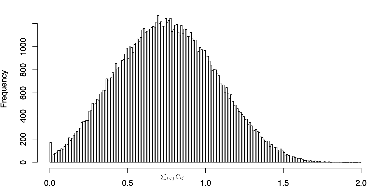
Refer to caption — Figure 1: In this figure, we present the frequency of the function $\sum_{i\leq j}C_{ij}$ for random pure states of four qubit states.

In Fig. 1, we present a histogram of the value of $\sum_{i\leq j}C_{ij}$ for random pure states of four qubits sampled uniformly. Here we find the function $MC(\cdot)$ mainly distributes in the section $[0,1.8],$ and in the section [1.8,2], there are few states. Fig. 1 supports Conjecture 1 for $n=4$ .

In Fig. 2, we present a histogram of the value of $\sum_{i\leq j}C_{ij}$ for random pure states of five qubits sampled uniformly. From the figure, we have that the sum of $MC(\cdot)$ mainly distributes in the section $[0,0.6]$ . In bai2007multipartite, the authors considered the multipartite correlations in four-qubit pure states. Here through the Fig 2, we have that the quantity of the bipartite correlations of most five-qubit pure states is few, then it seems that comparing with the separable states, the set of the entangled states for five-qubit pure states are bigger.

At the last of this section, we consider the $MC(\cdot)$ for a class of pure states in a system with more qubits studied in [34]. They are useful kinds of entanglement states for quantum teleportation and error correction,

\displaystyle|\psi\rangle=a|GHZ\rangle_{m}|W\rangle_{n}+b|W\rangle_{m}|GHZ\rangle_{n}.

Here $|a|^{2}+|b|^{2}=1,$ and $m,n\geq 2$ . Due to the shape of $|\psi\rangle$ , we have the set of the bipartite reduced density matrices for the pure state $|\psi\rangle$ consist of three kinds:

$\displaystyle\rho^{1}=$	$\displaystyle\frac{\|a\|^{2}}{2}(\|00\rangle\langle 00\|+\|11\rangle\langle 11\|)+\frac{\|b\|^{2}}{m}[(m-2)\|00\rangle\langle 00\|+(\|01\rangle+\|10\rangle)(\langle 01\|+\langle 10\|)],$
$\displaystyle\rho^{2}=$	$\displaystyle\frac{\|b\|^{2}}{2}(\|00\rangle\langle 00\|+\|11\rangle\langle 11\|)+\frac{\|a\|^{2}}{n}[(n-2)\|00\rangle\langle 00\|+(\|01\rangle+\|10\rangle)(\langle 01\|+\langle 10\|)],$
$\displaystyle\rho^{3}=$	$\displaystyle(\frac{a}{\sqrt{2n}}\|01\rangle+\frac{b}{\sqrt{2m}}\|10\rangle)(\frac{\overline{a}}{\sqrt{2n}}\langle 01\|+\frac{\overline{b}}{\sqrt{2m}}\langle 10\|)+[\frac{(n-1)\|a\|^{2}}{2n}+\frac{(m-1)\|b\|^{2}}{2m}]\|00\rangle\langle 00\|+\frac{(n-1)\|a\|^{2}}{2n}\|10\rangle\langle 10\|$
$\displaystyle+$	$\displaystyle\frac{\|a\|^{2}}{2n}\|11\rangle\langle 11\|+\frac{(m-1)\|b\|^{2}}{2m}\|01\rangle\langle 01\|+\frac{\|b\|^{2}}{2m}\|11\rangle\langle 11\|,$	(18)

then we have

	$\displaystyle C(\rho^{1})$
$\displaystyle=$	$\displaystyle\mathop{\rm max}\{0,\frac{2\|b\|^{2}}{m}-2\sqrt{\frac{\|a\|^{2}}{2}(\frac{\|a\|^{2}}{2}+\frac{m-2}{m}\|b\|^{2})}\}$
$\displaystyle=$	$\displaystyle\begin{cases}0&\|a\|^{2}\in(g(m),1],\\ \frac{2\|b\|^{2}}{m}-2\sqrt{\frac{\|a\|^{2}}{2}(\frac{\|a\|^{2}}{2}+\frac{m-2}{m}\|b\|^{2})}&\|a\|^{2}\in[0,g(m)]\end{cases}$	(19)
	$\displaystyle C(\rho^{2})$
$\displaystyle=$	$\displaystyle\mathop{\rm max}\{0,\frac{2\|a\|^{2}}{n}-2\sqrt{\frac{\|b\|^{2}}{2}(\frac{\|b\|^{2}}{2}+\frac{n-2}{n}\|a\|^{2})}\}$
$\displaystyle=$	$\displaystyle\begin{cases}0&\|a\|^{2}\in[0,h(n)]\\ \frac{2\|a\|^{2}}{n}-2\sqrt{\frac{\|b\|^{2}}{2}(\frac{\|b\|^{2}}{2}+\frac{n-2}{n}\|a\|^{2})}&\|a\|^{2}\in[h(n),1]\end{cases}$	(20)
	$\displaystyle C(\rho^{3})=0.$	(21)

Here $g(m)=\frac{m^{2}-2m+4-m\sqrt{m^{2}-4m+8}}{(m-2)^{2}},h(n)=\frac{n\sqrt{n^{2}-4n+8}-2n}{(n-2)^{2}}$ .

Let $x=|a|^{2}$ , $f(x)=MC(|\psi\rangle)$ . First we will compute the maximum when $(m,n)\in\{(2,2),(2,3),(3,2),(3,3),(2,4),(4,2)\}$ .

When $m=n=2,$ we have

\displaystyle f(x)=\begin{cases}1-2x&x\in[0,1/2]\\ 2x-1&x\in[1/2,1]\\ \end{cases},

(22)

then the maximum is 1, when $x=0$ or $1.$

When $m=2,n=3$ , we have

\displaystyle f(x)=\begin{cases}1-2x&x\in(0,1/2)\\ 0&x\in[1/2,3\sqrt{5}-6]\\ {2x}-\sqrt{3x^{2}-12x+9}&x\in(3\sqrt{5}-6,1],\end{cases}

(23)

then we have when $x=1$ , $f(x)$ gets the maximum $2$ .

When $m=3,n=2$ , we have

\displaystyle f(x)=\begin{cases}2(1-x)-\sqrt{3x(x+2)}&x\in[0,7-3\sqrt{5}]\\ 0&x\in[7-3\sqrt{5},\frac{1}{2}]\\ 2x-1&x\in[1/2,1],\end{cases}

(24)

when $x=0$ , $f(x)$ gets the maximum 2.

When $m=n=3,$ we have

\displaystyle f(x)=\begin{cases}3(1-x)-\sqrt{3{x(x+2)}}&x\in[0,7-3\sqrt{5}]\\ 0&x\in(7-3\sqrt{5},3\sqrt{5}-6)\\ 2x-\sqrt{3x^{2}-12x+9}&x\in(3\sqrt{5}-6,1],\end{cases}

(25)

when $x=0$ or $x=1,$ $f(x)$ gets the maximum, $2.$
When $m=4,n=2$ , we have

\displaystyle f(x)=\begin{cases}3-3x-6\sqrt{x}&x\in[0,3-2\sqrt{2}]\\ 0&x\in[3-2\sqrt{2},1/2]\\ 2x-1&x\in[1/2,1],\end{cases}

(26)

when $x=0$ , $f(x)$ gets the maximum, $3.$
When $m=2,$ $n=4$ , we have

\displaystyle f(x)=\begin{cases}1-2x&x\in[0,1.2]\\ 0&x\in(1/2,2\sqrt{2}-2)\\ 3x-12\sqrt{\frac{1}{4}-\frac{x}{4}}&x\in[2\sqrt{2}-2,1]\end{cases},

(27)

then $\mathop{\rm max}_{x\in[0,1]}f(x)=3.$
Next from simple computation, we have $\forall m,n\geq 3,$ $h(n)\geq g(m),$ then

		$\displaystyle f(x)$
	$\displaystyle=$	$\displaystyle\begin{cases}(m-1)(1-x)-2\sqrt{\frac{4-m}{4m}x^{2}+\frac{m-2}{2m}x}&x\in[0,g(m)]\\ 0&x\in[g(m),h(n)]\\ (n-1)x-n(n-1)\sqrt{\frac{1}{4}-\frac{x}{n}+\frac{4-n}{4n}x^{2}}&x\in(g(n),1)\end{cases}$		(28)

when $x\in[0,g(m)],m\geq 4,$ $f(x)$ is monotone decreasing, then when $x=0,$ $f(x)=m-1,$ when $x\in(g(n),1)$ $f(x)$ is monotone increasing, then $\mathop{\rm max}_{x\in(g(n,1))}f(x)=n-1,$ that is, when $m\geq 4,$ $f(x)=\mathop{\rm max}(m-1,n-1)$ .

In the next section, we present some applications of our results.

IV application

The structure of a multipartite entanglement system is complex. In this section, we apply our results above on the genuine entanglement detection. We also make some comments on the abosolutely maximally entangled states (AMES), and we apply Theorem 3 to present when a pure state is AMES in a three-qubit system.

IV.1 An entanglement criterion for genuine entangled states

On the other hand, an important problem in entanglement theory is to determine whether a multipartite state is genuinely entangled, biseparable or fully separable. An widely accepted method for attacking the problem is to construct entanglement witnesses (EWs) horodecki2009quantum. The EW $W$ is an Hermitian operator when $\mathop{\rm Tr}(W\sigma)\geq 0$ for every biseparable state $\sigma$ , and $\mathop{\rm Tr}(W\rho)<0$ for some entangled state $\rho$ . The EW is a theoretical and experimental method compared with mathematical criteria, such as positive partial transpose (PPT) peres1996separability and computable cross norm rudolph2005further. For a review we refer readers to the papers horodecki2009quantum; guhne2009entanglement. EWs have been constructed to detect the entanglement of many physically realizable states, such as the GHZ diagonal states chen2018precise; chen2019hierarchy, GHZ-like state zhao2019efficient, noisy Dicke states chen2020noise. In the following we connect EWs to the $MC(\phi)$ .

In practice, we need analyze the change of $MC(\phi)$ of $n$ -qubit pure states $|\varphi\rangle$ under the white noise. Let $\rho(p)=p|\varphi\rangle\!\langle\varphi|+(1-p){1\over 2^{n}}I_{2^{n}}$ with $p\in(0,1)$ . By definition and simple computation, one can show that the $MC(\rho)$ monotonically increases with $p$ . As an example, we assume that $|\varphi\rangle$ is the $n$ -qubit W state. Hence

\displaystyle\rho(p)=p|W_{n}\rangle\!\langle W_{n}|+(1-p)\frac{I}{2^{n}},

(29)

here we can find that the state $(\ref{rp})$ is symmetric. From computation, we have

\displaystyle C(\rho_{i\neq j})=\mathop{\rm max}(0,\frac{2p}{n}-2\sqrt{\frac{(1-p)(n+3np-8p)}{16n}}),

(30)

that is, when

\displaystyle 16p^{2}-n^{2}(1-p)^{2}+4np(n-2)(p-1)>0,

(31)

MC(\rho)=(n-1)p-(n-1)\sqrt{n(1-p)(n+3np-8p)}.

When $n=3$ , from the analysis above, we have when $p\geq\frac{\sqrt{155}-5}{8},$ the state $\rho(p)$ is a genuinely entangled state. In chen2020noise, the authors showed when $p\leq\frac{\sqrt{3}}{8+\sqrt{3}},$ the state $\rho(p)$ is fully separable, there the authors present an optimal entanglement witness $\widehat{W}$ for the $\rho(p)$ when $n=3,$ the witness $\widehat{W}$ is written as

	$\displaystyle\widehat{W}=$	$\displaystyle\frac{1}{d}\|000\rangle\langle 000\|-[\|001\rangle(\langle 001\|$
	$\displaystyle+$	$\displaystyle\langle 100\|)+\|010\rangle(\langle 001\|+\langle 100\|)$
	$\displaystyle+$	$\displaystyle\|100\rangle(\langle 001\|+\langle 010\|)]$
	$\displaystyle+$	$\displaystyle d(\|011\rangle+\|101\rangle+\|110\rangle)(\langle 011\|$
	$\displaystyle+$	$\displaystyle\langle 101\|+\langle 110\|).$

Ref. chen2012estimating has shown that the state $\rho(p)$ is fully separable when $p\leq\frac{\sqrt{3}}{8+\sqrt{3}},$ they also showed when $p\in(\frac{\sqrt{3}}{8+\sqrt{3}},0.2095],$ the state $\rho(p)$ is biseparable but not fully separable. Here if Conjecture 1 was true, then $MC(\rho)>n-2,$ implies that $\rho(p)$ is a genuinely entangled state. In particular, this is true when $n=3$ by Theorem 4. Thus proving Conjecture 1 is meaningful to the investigation of entanglement dectection.

IV.2 absolutely maximally entangled state

Next we investigate an absolutely maximally entangled states (AMES) in $n$ -qubit systems. A pure multipartite entangled state is called AMES if all reduced density operators obtained by tracing out at least half of the particles are maximally mixed goyeneche2015absolutely. So the function $MC(\cdot)$ of every AMES is zero, though the converse fails because the $n$ -qubit non-AMES state may have separable reduced density operators. An example is the GHZ state. Hence, we have constructed a necessary condition by which a multipartite state is an AMES. Next we consider the AMES in a $3$ -qubit system.

Corollary 1

The sole class of AMES $|\psi\rangle$ in an $3$ -qubit system are the states that are LU equivalent to $|GHZ\rangle=\frac{1}{\sqrt{2}}(|000\rangle+|111\rangle).$

We place the proof of the corollary in the APPENDIX VI.5.

IV.3 An upper bound of the sum of all bipartite quantum discord

Here we present an upper bound of the sum of all bipartite quantum discord for a three-qubit pure state. The quantum discord was first presented by Henderson and Vedral henderson2001classical, Ollivier and Zurek ollivier2001quantum independently. Quantum discord is a measure of nonclassical correlation. It is defined as

	$\displaystyle\delta_{AB}^{\leftarrow}=$	$\displaystyle I_{AB}-J_{AB}^{\leftarrow}$
	$\displaystyle=$	$\displaystyle I_{AB}-\mathop{\rm max}_{\{\Pi_{x}^{B}\}}(S(\rho_{A})-\sum_{x}p_{x}S(\rho_{A}^{x})),$

where the maximum takes over all the positive-operator-valued-measurements $\{\Pi_{x}^{B}\}$ performed on the subsystem B, $p_{x}=\mathop{\rm Tr}{\Pi_{x}^{B}\rho_{AB}\Pi_{x}^{B}},$ and $\rho_{A}^{x}=\mathop{\rm Tr}_{B}(\Pi_{x}^{B}\rho_{AB}\Pi_{x}^{B})/p_{x}.$ From its definition, it quantifies at least how much a bipartite state of one system is changed on anverage by the measurement of the other system. In the last decade, there are some results suggesting that quantum discord plays an important role in quantum information and computation tasks dakic2012quantum; gu2012observing; pirandola2014quantum; liu2017resource; liu2020quantum. Recently, Guo $et$ $al.$ considered the complete monogamy relation for multi-party quantum discord guo2021monogamy.

Next we recall a conservation law for distributed EoF and quantum discord of a three-qubit pure state fanchini2011conservation ,

\displaystyle E_{AB}+E_{AC}=

\displaystyle\delta_{AB}^{\leftarrow}+\delta_{AC}^{\leftarrow},

(32)

The law depends on the Koashi-Winter (KW) relation $E_{AB}+J_{AC}^{\leftarrow}=S_{A}$ koashi2004monogamy.
Here we present an upper bound of the sum of all the bipartite discord for a three-qubit pure state, from equation $(\ref{ced})$ , we have

		$\displaystyle\delta_{AB}^{\leftarrow}+\delta_{BC}^{\leftarrow}+\delta_{CA}^{\leftarrow}+\delta_{BA}^{\leftarrow}+\delta_{AC}^{\leftarrow}+\delta_{CB}^{\leftarrow}$
	$\displaystyle=$	$\displaystyle E_{AB}+E_{AC}+E_{BC}+E_{BA}+E_{CA}+E_{CB}$
	$\displaystyle\leq$	$\displaystyle 2\times c_{max}=2c_{max},$

Thus we have quantum discord owns a multi-linear monogamy relation for a three-qubit pure state.

V Conclusions

Here we have mainly considered the shareablility of the entanglement for a multi-qubit state in terms of the EoF. We have presented that up to the local unitary transformations, the W state is the unique that can reach the upper bound of $MC(\cdot)$ for a three-qubit state, these results may tell us that the entanglement cannot be shared freely for a three-qubit system. We have also picked $10^{5}$ four-qubit and five-qubit pure states randomly and computed their $MC(\cdot)$ , which have verified the Conjecture 1 numerically. Finally, we also have presented some applications of our results. We think the methods here we used can be generalized to consider the upper bound of the multi-linear monogamy relation in terms of other bipartite entanglement measures such as, R $\acute{e}$ nyi entanglement for an $n$ -qubit pure state. We believe that our results are helpful on the study of monogamy relations for multipartite entanglement systems.

Acknowledgments

Authors were supported by the NNSF of China (Grant No. 11871089), and the Fundamental Research Funds for the Central Universities (Grant Nos. ZG216S2005).

References

(1) R. Horodecki, P. Horodecki, M. Horodecki, and K. Horodecki, “Quantum entanglement,” Reviews of modern physics, vol. 81, no. 2, p. 865, 2009.
(2) C. H. Bennett and S. J. Wiesner, “Communication via one-and two-particle operators on einstein-podolsky-rosen states,” Physical review letters, vol. 69, no. 20, p. 2881, 1992.
(3) C. H. Bennett, G. Brassard, C. Crépeau, R. Jozsa, A. Peres, and W. K. Wootters, “Teleporting an unknown quantum state via dual classical and einstein-podolsky-rosen channels,” Physical review letters, vol. 70, no. 13, p. 1895, 1993.
(4) Y. Shimoni, D. Shapira, and O. Biham, “Entangled quantum states generated by shor’s factoring algorithm,” Physical Review A, vol. 72, no. 6, p. 062308, 2005.
(5) B. M. Terhal, “Is entanglement monogamous?” IBM Journal of Research and Development, vol. 48, no. 1, pp. 71–78, 2004.
(6) M. Pawlowski, “Security proof for cryptographic protocols based only on the monogamy of bell’s inequality violations,” Physical Review A, vol. 82, no. 3, p. 032313, 2010.
(7) X. Yang, K. Wei, H. Ma, S. Sun, and L. Wu, “Measurement-device-independent entanglement-based quantum key distribution,” Physical Review A, vol. 93, no. 5, p. 052303, 2016.
(8) M. Tomamichel, S. Fehr, J. Kaniewski, and S. Wehner, “A monogamy-of-entanglement game with applications to device-independent quantum cryptography,” New Journal of Physics, vol. 15, no. 10, p. 103002, 2013.
(9) L. Gao, M. Junge, and N. Laracuente, “Heralded channel holevo superadditivity bounds from entanglement monogamy,” Journal of Mathematical Physics, vol. 59, no. 6, p. 062203, 2018.
(10) V. Coffman, J. Kundu, and W. K. Wootters, “Distributed entanglement,” Physical Review A, vol. 61, no. 5, p. 052306, 2000.
(11) C.-s. Yu and H.-s. Song, “Monogamy and entanglement in tripartite quantum states,” Physics Letters A, vol. 373, no. 7, pp. 727–730, 2009.
(12) M. Karczewski, D. Kaszlikowski, and P. Kurzyński, “Monogamy of particle statistics in tripartite systems simulating bosons and fermions,” Physical review letters, vol. 121, no. 9, p. 090403, 2018.
(13) T. J. Osborne and F. Verstraete, “General monogamy inequality for bipartite qubit entanglement,” Physical review letters, vol. 96, no. 22, p. 220503, 2006.
(14) Y.-K. Bai, Y.-F. Xu, and Z. Wang, “General monogamy relation for the entanglement of formation in multiqubit systems,” Physical review letters, vol. 113, no. 10, p. 100503, 2014.
(15) X.-N. Zhu and S.-M. Fei, “Entanglement monogamy relations of qubit systems,” Physical Review A, vol. 90, no. 2, p. 024304, 2014.
(16) S.-M. F. Xue-na Zhu, “Generalized monogamy relations of concurrence for n-qubit systems,” Physical Review A, vol. 92, no. 6, p. 062345, 2015.
(17) J. San Kim, “Generalized entanglement constraints in multi-qubit systems in terms of tsallis entropy,” Annals of Physics, vol. 373, pp. 197–206, 2016.
(18) Z.-X. Jin, J. Li, T. Li, and S.-M. Fei, “Tighter monogamy relations in multiqubit systems,” Physical Review A, vol. 97, no. 3, p. 032336, 2018.
(19) C.-s. Yu, D.-m. Li, and N.-n. Zhou, “Monogamy of finite-dimensional entanglement induced by coherence,” EPL (Europhysics Letters), vol. 125, no. 5, p. 50001, 2019.
(20) T. Zhang, X. Huang, and S.-M. Fei, “Note on product-form monogamy relations for nonlocality and other correlation measures,” Journal of Physics A: Mathematical and Theoretical, vol. 53, no. 15, p. 155304, 2020.
(21) T. R. De Oliveira, M. F. Cornelio, and F. F. Fanchini, “Monogamy of entanglement of formation,” Physical Review A, vol. 89, no. 3, p. 034303, 2014.
(22) F. Liu, F. Gao, and Q.-Y. Wen, “Linear monogamy of entanglement in three-qubit systems,” Scientific reports, vol. 5, p. 16745, 2015.
(23) M. F. Cornelio, “Multipartite monogamy of the concurrence,” Physical Review A, vol. 87, no. 3, p. 032330, 2013.
(24) W. Dür, G. Vidal, and J. I. Cirac, “Three qubits can be entangled in two inequivalent ways,” Physical Review A, vol. 62, no. 6, p. 062314, 2000.
(25) J. Joo, Y.-J. Park, S. Oh, and J. Kim, “Quantum teleportation via a w state,” New Journal of Physics, vol. 5, no. 1, p. 136, 2003.
(26) H. Ng and K. Kim, “Quantum estimation of magnetic-field gradient using w-state,” Optics Communications, vol. 331, pp. 353–358, 2014.
(27) N. Yu, C. Guo, and R. Duan, “Obtaining a w state from a greenberger-horne-zeilinger state via stochastic local operations and classical communication with a rate approaching unity,” Physical review letters, vol. 112, no. 16, p. 160401, 2014.
(28) M. K. Vijayan, A. P. Lund, and P. P. Rohde, “A robust w-state encoding for linear quantum optics,” Quantum, vol. 4, p. 303, 2020.
(29) W. K. Wootters, “Entanglement of formation of an arbitrary state of two qubits,” Physical Review Letters, vol. 80, no. 10, p. 2245, 1998.
(30) A. Acin, D. Bruß, M. Lewenstein, and A. Sanpera, “Classification of mixed three-qubit states,” Physical Review Letters, vol. 87, no. 4, p. 040401, 2001.
(31) J. San Kim, A. Das, and B. C. Sanders, “Entanglement monogamy of multipartite higher-dimensional quantum systems using convex-roof extended negativity,” Physical Review A, vol. 79, no. 1, p. 012329, 2009.
(32) M. Koashi, V. Bužek, and N. Imoto, “Entangled webs: Tight bound for symmetric sharing of entanglement,” Physical Review A, vol. 62, no. 5, p. 050302, 2000.
(33) Y.-K. Bai, D. Yang, and Z. Wang, “Multipartite quantum correlation and entanglement in four-qubit pure states,” Physical Review A, vol. 76, no. 2, p. 022336, 2007.
(34) A. Peres, “Separability criterion for density matrices,” Physical Review Letters, vol. 77, no. 8, p. 1413, 1996.
(35) O. Rudolph, “Further results on the cross norm criterion for separability,” Quantum Information Processing, vol. 4, no. 3, pp. 219–239, 2005.
(36) O. Gühne and G. Tóth, “Entanglement detection,” Physics Reports, vol. 474, no. 1-6, pp. 1–75, 2009.
(37) X.-Y. Chen, L.-Z. Jiang, and Z.-A. Xu, “Precise detection of multipartite entanglement in four-qubit greenberger–horne–zeilinger diagonal states,” Frontiers of Physics, vol. 13, no. 5, p. 130317, 2018.
(38) X.-y. Chen and L.-z. Jiang, “A hierarchy of entanglement criteria for four-qubit symmetric greenberger–horne–zeilinger diagonal states,” Quantum Information Processing, vol. 18, no. 9, p. 262, 2019.
(39) Q. Zhao, G. Wang, X. Yuan, and X. Ma, “Efficient and robust detection of multipartite greenberger-horne-zeilinger-like states,” Physical Review A, vol. 99, no. 5, p. 052349, 2019.
(40) X.-y. Chen and L.-z. Jiang, “Noise tolerance of dicke states,” Physical Review A, vol. 101, no. 1, p. 012308, 2020.
(41) Z.-H. Chen, Z.-H. Ma, O. Gühne, and S. Severini, “Estimating entanglement monotones with a generalization of the wootters formula,” Physical review letters, vol. 109, no. 20, p. 200503, 2012.
(42) D. Goyeneche, D. Alsina, J. I. Latorre, A. Riera, and K. Życzkowski, “Absolutely maximally entangled states, combinatorial designs, and multiunitary matrices,” Physical Review A, vol. 92, no. 3, p. 032316, 2015.
(43) L. Henderson and V. Vedral, “Classical, quantum and total correlations,” Journal of physics A: mathematical and general, vol. 34, no. 35, p. 6899, 2001.
(44) H. Ollivier and W. H. Zurek, “Quantum discord: a measure of the quantumness of correlations,” Physical review letters, vol. 88, no. 1, p. 017901, 2001.
(45) B. Dakić, Y. O. Lipp, X. Ma, M. Ringbauer, S. Kropatschek, S. Barz, T. Paterek, V. Vedral, A. Zeilinger, Č. Brukner, et al., “Quantum discord as resource for remote state preparation,” Nature Physics, vol. 8, no. 9, pp. 666–670, 2012.
(46) M. Gu, H. M. Chrzanowski, S. M. Assad, T. Symul, K. Modi, T. C. Ralph, V. Vedral, and P. K. Lam, “Observing the operational significance of discord consumption,” Nature Physics, vol. 8, no. 9, pp. 671–675, 2012.
(47) S. Pirandola, “Quantum discord as a resource for quantum cryptography,” Scientific reports, vol. 4, p. 6956, 2014.
(48) Z.-W. Liu, X. Hu, and S. Lloyd, “Resource destroying maps,” Physical review letters, vol. 118, no. 6, p. 060502, 2017.
(49) R. Liu, T. Shang, and J.-w. Liu, “Quantum network coding utilizing quantum discord resource fully,” Quantum Information Processing, vol. 19, no. 2, pp. 1–19, 2020.
(50) Y. Guo, L. Huang, and Y. Zhang, “Monogamy of quantum discord,” arXiv preprint arXiv:2103.00924, 2021.
(51) F. F. Fanchini, M. F. Cornelio, M. C. de Oliveira, and A. O. Caldeira, “Conservation law for distributed entanglement of formation and quantum discord,” Physical Review A, vol. 84, no. 1, p. 012313, 2011.
(52) M. Koashi and A. Winter, “Monogamy of quantum entanglement and other correlations,” Physical Review A, vol. 69, no. 2, p. 022309, 2004.
(53) Y. K. Bai, Y. F. Xu, and Z. D. Wang, “Hierarchical monogamy relations for the squared entanglement of formation in multipartite systems,” Physical Review A, vol. 90, no. 6, p. 062343, 2014.
(54) A. Acin, A. Andrianov, L. Costa, E. Jane, J. Latorre, and R. Tarrach, “Generalized schmidt decomposition and classification of three-quantum-bit states,” Physical Review Letters, vol. 85, no. 7, p. 1560, 2000.
(55) G. W. Allen, O. Bucicovschi, and D. A. Meyer, “Entanglement constraints on states locally connected to the greenberger-horne-zeilinger state,” arXiv preprint arXiv:1709.05004, 2017.
(56) B. Kraus, J. Cirac, S. Karnas, and M. Lewenstein, “Separability in 2 $\times$ n composite quantum systems,” Physical Review A, vol. 61, no. 6, p. 062302, 2000.
(57) B. Kraus, “Local unitary equivalence and entanglement of multipartite pure states,” Physical Review A, vol. 82, no. 3, p. 032121, 2010.

VI Appendix

VI.1 The proof of Theorem 1

For a three-qubit pure state, the W state reaches the upper bound of multi-linear monogamy relation in terms of EoF.

Proof.

Here we denote that

$\displaystyle f(x)=$	$\displaystyle h(\frac{1+\sqrt{1-x}}{2})$
$\displaystyle x=$	$\displaystyle C^{2}_{AB}$
$\displaystyle y=$	$\displaystyle C^{2}_{AC}+C^{2}_{AB},$
$\displaystyle c=$	$\displaystyle C^{2}_{AC}+C^{2}_{AB}+C^{2}_{BC},$
$\displaystyle g(x,y)=$	$\displaystyle f(x)+f(y-x)+f(c-y),$	(34)
$\displaystyle\frac{\partial g}{\partial x}=$	$\displaystyle f^{{}^{\prime}}(x)-f^{{}^{\prime}}(y-x)=0,$
$\displaystyle\frac{\partial g}{\partial y}=$	$\displaystyle f^{{}^{\prime}}(y-x)-f^{{}^{\prime}}(c-y)=0.$	(35)

As $f^{{}^{\prime\prime}}(x)<0,$ $f^{{}^{\prime}}(x)$ is monotonously decreasing bai2014hierarchical, $-f^{{}^{\prime}}(y-x)$ is also monotonously decreasing in terms of $x$ , and by the equality (35), we have

\displaystyle C^{2}_{AB}=C^{2}_{AC}=C^{2}_{BC}

(36)

is the only case when the $(\ref{pf})$ is valid. Furthermore, as $f(x)$ is a monotonic function bai2014hierarchical, we have when $(\ref{fc2})$ is valid, $E(\rho_{AB})+E(\rho_{AC})+E(\rho_{BC})$ achieves the upper bound for a three-qubit pure state.
From acin2000generalized, we have that a three-qubit pure state $|\psi\rangle_{ABC}$ can be written in the generalized Schmidt decomposition:

\displaystyle|\psi\rangle=l_{0}|000\rangle+l_{1}e^{i\theta}|100\rangle+l_{2}|101\rangle+l_{3}|110\rangle+l_{4}|111\rangle,

(37)

here $\theta\in[0,\pi),l_{i}\geq 0,i=0,1,2,3,4,\sum_{i=0}^{4}l_{i}^{2}=1.$ From simple computation, we have

	$\displaystyle C_{AB}^{2}=$	$\displaystyle 4l_{0}^{2}l_{2}^{2},C_{AC}^{2}=4l_{0}^{2}l_{3}^{2},$		(38)
	$\displaystyle C_{BC}^{2}=$	$\displaystyle 4l_{2}^{2}l_{3}^{2}+4l_{1}^{2}l_{4}^{2}-8l_{1}l_{2}l_{3}l_{4}cos\theta.$		(39)

As $f(x)$ is monotone bai2014hierarchical, then we only need to obtain the maximum of $4l_{0}^{2}l_{2}^{2}$ by using the Lagrange multiplier,

		$\displaystyle m(l_{0},l_{1},l_{2},l_{4},\lambda,\mu)=4l_{0}^{2}l_{2}^{2}+\lambda(l_{0}^{2}+l_{1}^{2}+2l_{2}^{2}+l_{4}^{2}-1),$
		$\displaystyle+\mu(l_{0}^{2}l_{2}^{2}-l_{2}^{4}-l_{1}^{2}l_{4}^{2}+2l_{1}l_{2}^{2}l_{4}\cos\theta),$		(40)
		$\displaystyle\frac{\partial m}{\partial l_{0}}=8l_{0}l_{2}^{2}+2\lambda l_{0}+2\mu l_{0}l_{2}^{2},$		(41)
		$\displaystyle\frac{\partial m}{\partial l_{1}}=2\lambda l_{1}+2\mu l_{2}^{2}l_{4}\cos\theta-2\mu l_{1}l_{4}^{2},$		(42)
		$\displaystyle\frac{\partial m}{\partial l_{2}}=8l_{0}^{2}l_{2}+4\lambda l_{2}+2\mu l_{0}^{2}l_{2}-4\mu l_{2}^{3}+4\mu l_{1}l_{2}l_{4}\cos\theta,$		(43)
		$\displaystyle\frac{\partial m}{\partial l_{4}}=2\lambda l_{4}-2\mu l_{1}^{2}l_{4}+2\mu l_{1}l_{2}^{2}\cos\theta,$		(44)
		$\displaystyle\frac{\partial m}{\partial\theta}=-2\mu l_{1}l_{2}^{2}l_{4}\sin\theta,$		(45)
		$\displaystyle\frac{\partial m}{\partial\lambda}=l_{0}^{2}+l_{1}^{2}+2l_{2}^{2}+l_{4}^{2}-1,$		(46)
		$\displaystyle\frac{\partial m}{\partial\mu}=l_{0}^{2}l_{2}^{2}-l_{2}^{4}-l_{1}^{2}l_{4}^{2}+2l_{1}l_{2}^{2}l_{4}\cos\theta,$		(47)

when the fomulas $(\ref{f1})-(\ref{f7})$ equal to 0, we have $l_{0}=l_{2}=l_{3}=\frac{1}{\sqrt{3}},l_{1}=l_{4}=0$ is the only case when $C^{2}(\rho_{AB})$ attains the maximum, that is,

		$\displaystyle\mathop{\rm max}_{\|\psi\rangle_{ABC}}(E(\rho_{AB})+E(\rho_{AC})+E(\rho_{BC}))$
	$\displaystyle:=$	$\displaystyle c_{max}=3h(\frac{1}{2}+\frac{\sqrt{5}}{6}).$		(48)

When computing $(\ref{f1})-(\ref{f7})$ equal to 0, according to $(\ref{f5})$ , we have that at least one of the equalities in the set $\{\mu=0,l_{1}=0,l_{2}=0,l_{4}=0,\sin\theta=0\}$ is valid. Then by using the method of exclusion, we could get the result. By the way, in the method of exclusion, we mainly use that when $|\psi\rangle$ is separable, the function $ME(\cdot)$ cannot get the maximum.
When we take the operation $\sigma_{x}$ on the first system, we get the $W$ state $\frac{1}{\sqrt{3}}(|001\rangle+|010\rangle+|100\rangle).$
$\sqcap$ $\sqcup$

VI.2 The proof of Lemma 1

Up to the local unitary transformations, the W state is the unique state that can reach the upper bound in terms of the function $MC(\psi)=C_{AB}+C_{BC}+C_{AC}$ for a three-qubit pure state.

Proof.

We’ll compute the maximum of the six classes of a three-qubit state respectively according to allen2017entanglement.
$Case$ $i$ : When $|\psi\rangle_{ABC}$ is $A-B-C$ , $MC(\psi)=0$ .
$Case$ $ii$ : When $|\psi\rangle_{ABC}$ is biseparable, if $|\psi\rangle_{ABC}=|\phi_{1}\rangle_{A}\otimes|\phi_{2}\rangle_{BC}$ , $C_{AB}=C_{AC}=0$ , $MC(\psi)=C_{BC}\leq 1$ , the other cases are similar.
$Case$ $iii$ : When $|\psi\rangle_{ABC}$ belongs to the $W$ class, according to the fomula $(\ref{LUW}),$ $MC(\psi)=2r_{2}r_{3}+2r_{1}r_{3}+2r_{1}r_{2}$ . Trivially, when $r_{1}=r_{2}=r_{3}$ , that is, $|\psi\rangle_{ABC}=|W\rangle=\frac{1}{\sqrt{3}}(|001\rangle+|010\rangle+|110\rangle)$ , $MC(\psi)$ gets the maximum.
$Case$ $iv$ : When $|\psi\rangle_{ABC}$ belongs to the $GHZ$ class, according to allen2017entanglement, assume $|\psi\rangle=M_{1}\otimes M_{2}\otimes M_{3}|GHZ\rangle$ , $M_{i}=\big(\vec{u_{i}},\vec{v_{i}}\big)$ , $\vec{u_{i}}=(u_{i}\cos\theta_{i},u_{i}\sin\theta_{i})^{T}$ , $\vec{v_{i}}=(v_{i}\cos(\phi_{i}+\theta_{i}),v_{i}\sin(\phi_{i}+\theta_{i}))^{T}$ ,

\displaystyle MC(\psi)=\frac{|c_{1}s_{2}s_{3}|+|c_{2}s_{1}s_{3}|+|c_{3}s_{1}s_{2}|}{r+c_{1}c_{2}c_{3}},

(49)

here we denote $c_{i}=\cos\phi_{i},s_{i}=\sin\phi_{i},i=1,2,3$ , $2r=\frac{u_{1}u_{2}u_{3}}{v_{1}v_{2}v_{3}}+\frac{v_{1}v_{2}v_{3}}{u_{1}u_{2}u_{3}}$ , $r\geq 1$ . In order to let $MC$ be the maximum, assume $r=1$ . When $c_{i}<0$ , $MC$ will gets maximum. then let $\phi_{i}\in[0,\frac{\pi}{2}],MC(\psi)=\frac{c_{1}s_{2}s_{3}+c_{2}s_{1}s_{3}+c_{3}s_{1}s_{2}}{1-c_{1}c_{2}c_{3}}$ . Next we will prove $MC(\psi)\leq 2$ , first we define $l(c_{1},c_{2},c_{3})$ as follows,

		$\displaystyle l(c_{1},c_{2},c_{3})$
	$\displaystyle=$	$\displaystyle c_{1}\cos(\phi_{2}-\phi_{3})+c_{2}\cos(\phi_{1}-\phi_{3})+c_{3}\cos(\phi_{1}-\phi_{2})$
	$\displaystyle-$	$\displaystyle c_{1}c_{2}c_{3},$

assume $c_{1}>c_{2}\geq c_{3}$ , then we obtain

\displaystyle l(c_{1},c_{2},c_{3})\leq l(c_{1},c_{1},c_{1}).

When $c_{1}=c_{2}=c_{3}$ , the function $l(c_{1},c_{1},c_{1})$ is a monotonic function of $c_{1}$ . When $c_{1}\rightarrow 1$ , the function $l(c_{1},c_{1},c_{1})$ gets the maximum, that is, $MC(\psi)\rightarrow 2$ . Then we prove that if $|\psi\rangle_{ABC}$ is a GHZ class state, then $MC(|\psi\rangle_{ABC})\leq 2.$ However, from the above analysis, when $MC(|\psi\rangle_{ABC})=2,$ we have $c_{1}=c_{2}=c_{3}\rightarrow 1,$ that is, the matrix $M_{i}$ is sigular, this is impossible.

$\sqcap$ $\sqcup$

VI.3 The proof of Theorem 2

Up to the local unitary transformations, the W state is the unique state that can reach the upper bound in terms of the function $MC(\cdot)$ for a three-qubit state.

Proof.

Combining with Lemma 1, we only need to present that the mixed states cannot reach the upper bound of the multi-linear monogamy relations in terms of concurrence.
Due to Lemma 1, for a three-qubit pure state $|\psi\rangle,$ $MC(|\psi\rangle)$ gets the maximum, only when $|\psi\rangle$ is LU equivalent to $|W\rangle$ . Assume $\rho$ is a three-qubit mixed system, $\{(p_{i},|\phi_{i}\rangle)|i=1,2,\cdots,k\}$ is an optimal decompostion of $\rho$ , we can always assume $k=2.$ For the cases when $k>2,$ we can prove similarly. As $|\phi_{i}\rangle$ is LU equivalent to $|W\rangle$ , we can always assume $\{(p_{1},|W\rangle),(p_{2},U_{1}\otimes U_{2}\otimes U_{3}|W\rangle)\}$ is a decompostion of $\rho,$ then

	$\displaystyle MC(\rho)=$	$\displaystyle C(\rho_{AB})+C(\rho_{AC})+C(\rho_{BC})$
	$\displaystyle=$	$\displaystyle C(\sigma_{1})+C(\sigma_{2})+C(\sigma_{3})$

here we assume

	$\displaystyle\sigma_{1}=$	$\displaystyle\frac{p_{1}}{3}(\|00\rangle\langle 00\|+2\|\phi^{+}\rangle\langle\phi^{+}\|)+\frac{p_{2}}{3}\tau_{1},$
	$\displaystyle\sigma_{2}=$	$\displaystyle\frac{p_{1}}{3}[\|00\rangle\langle 00\|+2\|\phi^{+}\rangle\langle\phi^{+}\|]+\frac{p_{2}}{3}\tau_{2},$
	$\displaystyle\sigma_{3}=$	$\displaystyle\frac{p_{1}}{3}[\|00\rangle\langle 00\|+2\|\phi^{+}\rangle\langle\phi^{+}\|]+\frac{p_{2}}{3}\tau_{3},$
	$\displaystyle\|\phi^{+}\rangle=$	$\displaystyle\frac{1}{\sqrt{2}}(\|01\rangle+\|10\rangle),$

here we denote $\tau_{1}=[(U_{1}\otimes U_{2})|00\rangle\langle 00|(U_{1}\otimes U_{2})^{\dagger}+2(U_{1}\otimes U_{2})|\phi^{+}\rangle\langle\phi^{+}|(U_{1}\otimes U_{2})^{\dagger}],$ $\tau_{2}=[(U_{1}\otimes U_{3})|00\rangle\langle 00|(U_{1}\otimes U_{3})^{\dagger}+2(U_{1}\otimes U_{3})|\phi^{+}\rangle\langle\phi^{+}|(U_{1}\otimes U_{3})^{\dagger}],$ $\tau_{3}=[(U_{2}\otimes U_{3})|00\rangle\langle 00|(U_{2}\otimes U_{3})^{\dagger}+2(U_{2}\otimes U_{3})|\phi^{+}\rangle\langle\phi^{+}|(U_{2}\otimes U_{3})^{\dagger}],$ then we have

\displaystyle C(\sigma_{1})\leq\frac{2}{3}C(p_{1}|\phi^{+}\rangle\langle\phi^{+}|+p_{2}(U_{1}\otimes U_{2})|\phi^{+}\rangle\langle\phi^{+}|(U_{1}\otimes U_{2})^{\dagger}),

(51)

By the Lemma 2, 3 and 4, we have $(U_{1}\otimes U_{2})|\phi^{+}\rangle=e^{ix}|\phi^{+}\rangle$ is a sufficient and necessary condition of $C(p_{1}|\phi^{+}\rangle\langle\phi^{+}|+p_{2}(U_{1}\otimes U_{2})|\phi^{+}\rangle\langle\phi^{+}|(U_{1}\otimes U_{2})^{\dagger})=1,$ here $e^{ix}$ is a global phase factor. Then we can get the similar result for $\sigma_{2}$ and $\sigma_{3}.$ As $Sr(|01\rangle)=Sr(|10\rangle)=1$ , here we denote that $Sr(\cdot)$ is the schmidt rank, then we have $U_{i}=\left(\begin{array}[]{cc}e^{i\theta_{i}}&0\\ 0&1\end{array}\right),i=1,2,3$ , that is, $\rho=|W\rangle\langle W|.$ Then we finish the proof.
$\sqcap$ $\sqcup$

Here we will prove that $(U_{1}\otimes U_{2})|\phi^{+}\rangle=e^{ix}|\phi^{+}\rangle$ is a sufficient and necessary condition of $C(p_{1}|\phi^{+}\rangle\langle\phi^{+}|+p_{2}(U_{1}\otimes U_{2})|\phi^{+}\rangle\langle\phi^{+}|(U_{1}\otimes U_{2})^{\dagger})=1.$ As $\Longrightarrow$ is trivial,
$\Longleftarrow:$ First we will present a lemma.

Lemma 2

Assume $A,B\in Pos(\mathbb{H})$ , here we denote that $Pos(\mathbb{H})$ is a linear space consisting of all the semidefinite positive operators of a bounded Hilbert space $\mathbb{H}$ . Here we denote that $Eig(A)$ and $Eig(B)$ are two sets consisting of all the eigenvalues of the matrix $A$ and $B$ respectively. If the biggest elements in the set $Eig(A)$ and $Eig(B)$ are 1 or less, then the biggest element in the set $Eig(AB)$ is 1 or less.

Proof.

Assume that the eigenvalues of $A$ are $\lambda_{i}$ with its eigenvector $|\alpha_{i}\rangle$ , the eigenvalues of $B$ are $\mu_{j}$ with its eigenvector $|\beta_{j}\rangle$ , and the eigenvalues of $AB$ are $\chi_{k}$ with its eigenvectors $|\gamma_{k}\rangle$ . Here we always assume that the range of $A$ and $B$ are nonsingular, then we have

$\displaystyle AB\|\gamma_{k}\rangle=$	$\displaystyle AB\sum_{j}x_{jk}\|\beta_{j}\rangle$
$\displaystyle=$	$\displaystyle A\sum_{j}\mu_{j}x_{jk}\|\beta_{j}\rangle$
$\displaystyle=$	$\displaystyle\sum_{ij}\lambda_{i}\mu_{j}x_{jk}y_{ij}\|\alpha_{i}\rangle,$	(52)
$\displaystyle AB\|\gamma_{k}\rangle=$	$\displaystyle\chi_{k}\|\gamma_{k}\rangle$
$\displaystyle=$	$\displaystyle\chi_{k}\sum_{ij}x_{jk}y_{ij}\|\alpha_{i}\rangle,$	(53)

in the formula $(\ref{bet}),$ we denote that $|\gamma_{k}\rangle=\sum_{j}x_{jk}|\beta_{j}\rangle$ and $|\beta_{j}\rangle=\sum_{i}y_{ij}|\alpha_{i}\rangle.$ From the equality $(\ref{bet})$ and $(\ref{gamma}),$ we have

\displaystyle\chi_{k}=\frac{\sum_{ij}\lambda_{i}\mu_{j}x_{jk}y_{ij}}{\sum_{ij}x_{jk}y_{ij}}\leq 1.

(54)

here the $(\ref{chi})$ is due to $\lambda_{i}\leq 1$ and $\mu_{j}\leq 1$ . Then we finish the proof. $\sqcap$ $\sqcup$

As $\rho$ is semidefinite positive , then $(\sigma_{y}\otimes\sigma_{y})\overline{\rho}(\sigma_{y}\otimes\sigma_{y})$ is semidifinite positive, then due to the Lemma 2, we have that all the eigenvalues of $\rho(\sigma_{y}\otimes\sigma_{y})\overline{\rho}(\sigma_{y}\otimes\sigma_{y})$ are 1 or less. Then due to $(\ref{C2}),$ we have that only when $Rank(\rho(\sigma_{y}\otimes\sigma_{y})\overline{\rho}(\sigma_{y}\otimes\sigma_{y}))=1$ and $\lambda_{1}$ in $(\ref{C2})$ equals to 1 can $C(\rho)=1.$ As $\sigma_{y}\otimes\sigma_{y}$ is nonsigular, we only need $Rank(\rho)=1.$

Lemma 3

$Rank[p_{1}|\phi^{+}\rangle\langle\phi^{+}|+p_{2}(U_{1}\otimes U_{2})|\phi^{+}\rangle\langle\phi^{+}|(U_{1}\otimes U_{2})^{\dagger}]=1$ if and only if $(U_{1}\otimes U_{2})|\phi^{+}\rangle=e^{ix}|\phi^{+}\rangle,$ here $e^{ix}$ is a global phase factor.

Proof.

Here we denote $\sigma=p_{1}|\phi^{+}\rangle\langle\phi^{+}|+p_{2}(U_{1}\otimes U_{2})|\phi^{+}\rangle\langle\phi^{+}|(U_{1}\otimes U_{2})^{\dagger}.$ If $(U_{1}\otimes U_{2})|\phi^{+}\rangle\neq e^{ix}|\phi^{+}\rangle,$ then $(U_{1}\otimes U_{2})|\phi^{+}\rangle$ and $|\phi^{+}\rangle$ are linear independent, $dim(span\{|\phi^{+}\rangle,(U_{1}\otimes U_{2})|\phi^{+}\rangle\})=2,$ $dim(span\{|\phi^{+}\rangle,(U_{1}\otimes U_{2})|\phi^{+}\rangle\}^{\perp}=n-2.$ As $\forall|\alpha\rangle\in dim(span\{|\phi^{+}\rangle,(U_{1}\otimes U_{2})|\phi^{+}\rangle\}^{\perp},$ $\sigma|\alpha\rangle=0,$ that is, $Rank(\sigma)\leq 2.$ As we cannot find a nontrivial vector $|\beta\rangle$ in the subspace ${span\{|\phi^{+}\rangle,(U_{1}\otimes U_{2})|\phi^{+}\rangle\}}$ such that $\sigma|\beta\rangle=0,$ then we finish the proof. $\sqcap$ $\sqcup$

Lemma 4

Assume $\theta=p_{1}|\phi^{+}\rangle\langle\phi^{+}|+p_{2}U_{1}\otimes U_{2})|\phi^{+}\rangle\langle\phi^{+}|(U_{1}\otimes U_{2})^{\dagger}$ with $Rank(\theta)=2,$ then $Rank[(\sigma_{y}\otimes\sigma_{y})\tilde{\theta}(\sigma_{y}\otimes\sigma_{y})\theta]=2.$

Proof.

As $\sigma_{y}\otimes\sigma_{y}$ is invertible, we only need to prove $Rank[\tilde{\theta}(\sigma_{y}\otimes\sigma_{y})\theta]=2.$ As $Rank[\tilde{\theta}(\sigma_{y}\otimes\sigma_{y})\theta]=Rank[\theta\tilde{\theta}(\sigma_{y}\otimes\sigma_{y})],$ then if we can prove $Rank[\theta\tilde{\theta}]=2,$ we finish the proof. As $\theta=\theta^{\dagger},$ then $Rank[\theta\tilde{\theta}]=Rank[\theta\theta^{T}]=Rank(\theta)=2.$ $\sqcap$ $\sqcup$

VI.4 The proof of Theorem 3

Proof.

First we recall $MC(|\psi\rangle_{ABC})=C^{2}_{AB}+C_{AC}^{2}+C_{BC}^{2}.$
$\Leftarrow:$ When $|\psi\rangle=r_{0}|000\rangle+r_{1}|111\rangle$ , then $\rho_{AB}=\rho_{AC}=\rho_{BC}=r^{2}_{0}|00\rangle\langle 00|+r_{1}^{2}|11\rangle\langle 11|$ , $C(\rho_{AB})=C(\rho_{AC})=C(\rho_{BC})=0,$ that is, $MC(|\psi\rangle)=0.$
$\Rightarrow:$ In the proof of theroem 1, we present that for a three-qubit pure state $|\psi\rangle_{ABC}=l_{0}|000\rangle+l_{1}e^{i\theta}|100\rangle+l_{2}|101\rangle+l_{3}|110\rangle+l_{4}|111\rangle$ , here $l_{i}\geq 0,$ $i=0,1,2,3,4,$ $\theta\in[0,\pi),$

	$\displaystyle C_{AB}^{2}=$	$\displaystyle 4l_{0}^{2}l_{2}^{2},\hskip 5.69054ptC_{AC}^{2}=4l_{0}^{2}l_{3}^{2},$
	$\displaystyle C_{BC}^{2}=$	$\displaystyle 4l_{2}^{2}l_{3}^{2}+4l_{1}^{2}l_{4}^{2}-8l_{1}l_{2}l_{3}l_{4}\cos\theta.$		(55)

When $MC(|\psi\rangle)=0,$ we have that

	$\displaystyle l_{0}l_{2}=l_{0}l_{3}=0,$
	$\displaystyle l_{2}^{2}l_{3}^{2}+l_{1}^{2}l_{4}^{2}=2l_{1}l_{2}l_{3}l_{4}\cos\theta.$		(56)

When $l_{0}\neq 0,$ we have $l_{2}=l_{3}=0,$ that is, $l_{1}l_{4}=0,$ then $|\psi\rangle=l_{0}|000\rangle+l_{4}|111\rangle,$ or $|\psi\rangle=(l_{0}|0\rangle+l_{1}e^{i\theta}|1\rangle)|00\rangle.$ When $|\psi\rangle$ is the second state, let $U_{1}$ be a unitary on the first system such that $U_{1}(|l_{0}|0\rangle+l_{1}e^{i\theta}|1\rangle\rangle)=|0\rangle,$ then the second state is LU equivalent to the state $|000\rangle.$ Below we denote $U_{i}$ be a unitary on the $i$ -th system, $i=1,2,3$ .

When $l_{0}=0,$ then from the third formula in (55),

\displaystyle(l_{2}l_{3}\cos\theta-l_{1}l_{4})^{2}+l_{2}^{2}l_{3}^{2}(\sin\theta)^{2}=0,

(57)

that is, $l_{2}l_{3}\cos\theta=l_{1}l_{4},$ $l_{2}l_{3}\sin\theta=0.$ When $\sin\theta=0$ and $l_{i}\geq 0,$ $i=1,2,3,4,$ $\cos\theta=1.$ That is, $(l_{1},l_{2})=a(l_{3},l_{4}),$ then $|\psi\rangle=|1\rangle(|0\rangle+a|1\rangle)(l_{1}|0\rangle+l_{2}|1\rangle).$ When $U_{2}(|0\rangle+a|1\rangle)=\sqrt{1+a^{2}}|0\rangle,$ $U_{3}(l_{1}|0\rangle+l_{2}|1\rangle)=\sqrt{l_{1}^{2}+l_{2}^{2}}|0\rangle,$ then we obtain that the above state is LU equivalent to $|000\rangle.$ When $l_{2}=0,$ then $l_{1}l_{4}=0.$ If $l_{1}=0,$ then $|\psi\rangle$ can be represented as $|\phi_{1}\rangle=l_{3}|110\rangle+l_{4}|111\rangle.$ Let $U_{3}(l_{3}|0\rangle+l_{4}|1\rangle)=|1\rangle$ , then it is LU equivalent to the state $|111\rangle,$ If $l_{4}=0,$ then $|\psi\rangle$ can be represented as $|\phi_{2}\rangle=e^{i\theta}l_{1}|100\rangle+l_{3}|110\rangle$ . Let $U_{2}(e^{i\theta}l_{1}|0\rangle+l_{3}|1\rangle)=|1\rangle$ and $U_{3}=\sigma_{X}$ , then it is LU equivalent to the state $|111\rangle.$ The case when $l_{3}=0$ is similar to the case when $l_{2}=0.$ Then we finish the proof. $\sqcap$ $\sqcup$

VI.5 The proof of Corollary 1

The sole class of AMES $|\psi\rangle$ in an $3$ -qubit system are the states that are LU equivalent to $|GHZ\rangle=\frac{1}{\sqrt{2}}(|000\rangle+|111\rangle).$

Proof.

First we provide two methods to prove that $\rho_{AB}$ , $\rho_{AC}$ and $\rho_{BC}$ are separable. Assume $|\psi\rangle_{ABC}$ is an AMES state in an $3$ -qubit state, then

\rho_{A}=\rho_{B}=\rho_{C}=\frac{I}{2}.

Next as $\rho_{A}=\frac{I}{2},$ then any purification state $|\phi\rangle_{AB^{{}^{\prime}}}$ of $\rho_{A}$ can be written as

|\phi\rangle_{ABC}=(I_{A}\otimes U_{BC})\frac{(|00\rangle+|11\rangle)|0\rangle}{\sqrt{2}},

here $U_{BC}$ is a unitary operator, then we have

	$\displaystyle\rho_{BC}=\|\phi_{1}\rangle\langle\phi_{1}\|+\|\phi_{2}\rangle\langle\phi_{2}\|,$
	$\displaystyle\|\phi_{1}\rangle=U_{BC}\|00\rangle,\hskip 8.53581pt\|\phi_{2}\rangle=U_{BC}\|10\rangle$		(58)

that is, $r(\rho_{BC})=2,$ then due to Theorem 1 in kraus2000separability, we have $\rho_{BC}$ is separable. Similarly, we have $\rho_{AB}$ and $\rho_{AC}$ is separable.

Here we provide the other method to prove that $\rho_{AB},$ $\rho_{AC}$ and $\rho_{BC}$ are separable. As $\rho_{A}=\rho_{B}=\frac{I}{2},$ then from kraus2010local, we have

$\displaystyle\rho_{AB}=$	$\displaystyle\lambda_{1}\Psi^{+}+\lambda_{2}\Psi^{-}+\lambda_{3}\Phi^{+}+\lambda_{4}\Phi^{-},$	(59)
$\displaystyle\Psi^{+}=$	$\displaystyle\frac{1}{2}(\|00\rangle+\|11\rangle)(\langle 11\|+\langle 00\|),$
$\displaystyle\Psi^{-}=$	$\displaystyle\frac{1}{2}(\|00\rangle-\|11\rangle)(\|00\rangle-\langle 11\|),$
$\displaystyle\Phi^{+}=$	$\displaystyle\frac{1}{2}(\|01\rangle+\langle 10\|)(\langle 01\|+\langle 10\|),$
$\displaystyle\Phi^{-}=$	$\displaystyle\frac{1}{2}(\|01\rangle-\|10\rangle)(\langle 01\|-\langle 10\|).$

As $\rho_{C}$ and $\rho_{AB}$ are with the same spectrum, then we have only two of $\lambda_{i},$ $i=1,2,3,4$ are $\frac{1}{2}$ . Then $\rho_{AB}$ is separable. Similarly, we have $\rho_{AC}$ and $\rho_{BC}$ are separable.

As all of $\rho_{AB},$ $\rho_{AC}$ and $\rho_{BC}$ are separable, then we have

\displaystyle MC(|\psi\rangle)=0,

then from Theorem 3, we have $|\psi\rangle=r_{0}|000\rangle+r_{1}|111\rangle$ up to unitary operations when $r_{0},r_{1}\in[0,1].$ As $\rho_{A}=\rho_{B}=\rho_{C}=\frac{1}{2},$ then $|\psi\rangle=\frac{1}{2}(|000\rangle+|111\rangle)$ up to local unitary operations. $\sqcap$ $\sqcup$

$\displaystyle MC(\|\phi\rangle)=$	$\displaystyle 2p\sum_{i<j}\|a_{i}a_{j}\|$
$\displaystyle=$	$\displaystyle p[(\sum_{i}\|a_{i}\|)^{2}-\sum_{i}\|a_{i}\|^{2}]$
$\displaystyle=$	$\displaystyle p[(\sum_{i}\|a_{i}\|)^{2}-1].$	(16)

	$\displaystyle\sigma_{1}=$	$\displaystyle\frac{p_{1}}{3}(\|00\rangle\langle 00\|+2\|\phi^{+}\rangle\langle\phi^{+}\|)+\frac{p_{2}}{3}\tau_{1},$
	$\displaystyle\sigma_{2}=$	$\displaystyle\frac{p_{1}}{3}[\|00\rangle\langle 00\|+2\|\phi^{+}\rangle\langle\phi^{+}\|]+\frac{p_{2}}{3}\tau_{2},$
	$\displaystyle\sigma_{3}=$	$\displaystyle\frac{p_{1}}{3}[\|00\rangle\langle 00\|+2\|\phi^{+}\rangle\langle\phi^{+}\|]+\frac{p_{2}}{3}\tau_{3},$
	$\displaystyle\|\phi^{+}\rangle=$	$\displaystyle\frac{1}{\sqrt{2}}(\|01\rangle+\|10\rangle),$

$\displaystyle AB\|\gamma_{k}\rangle=$	$\displaystyle AB\sum_{j}x_{jk}\|\beta_{j}\rangle$
$\displaystyle=$	$\displaystyle A\sum_{j}\mu_{j}x_{jk}\|\beta_{j}\rangle$
$\displaystyle=$	$\displaystyle\sum_{ij}\lambda_{i}\mu_{j}x_{jk}y_{ij}\|\alpha_{i}\rangle,$	(52)
$\displaystyle AB\|\gamma_{k}\rangle=$	$\displaystyle\chi_{k}\|\gamma_{k}\rangle$
$\displaystyle=$	$\displaystyle\chi_{k}\sum_{ij}x_{jk}y_{ij}\|\alpha_{i}\rangle,$	(53)