Heterogeneous large datasets integration using Bayesian factor regression
Abstract
Two key challenges in modern statistical applications are the large amount of information recorded per individual, and that such data are often not collected all at once but in batches. These batch effects can be complex, causing distortions in both mean and variance. We propose a novel sparse latent factor regression model to integrate such heterogeneous data. The model provides a tool for data exploration via dimensionality reduction while correcting for a range of batch effects. We study the use of several sparse priors (local and non-local) to learn the dimension of the latent factors. Our model is fitted in a deterministic fashion by means of an EM algorithm for which we derive closed-form updates, contributing a novel scalable algorithm for non-local priors of interest beyond the immediate scope of this paper. We present several examples, with a focus on bioinformatics applications. Our results show an increase in the accuracy of the dimensionality reduction, with non-local priors substantially improving the reconstruction of factor cardinality, as well as the need to account for batch effects to obtain reliable results. Our model provides a novel approach to latent factor regression that balances sparsity with sensitivity and is highly computationally efficient.
Keywords: Bayesian factor analysis; EM; Non-local priors; Shrinkage
1 Introduction
A first important task when dealing with large datasets is to conduct an exploratory analysis. Dimensionality reduction techniques have proven a highly popular tool for this purpose. Those techniques provide a lower-dimensional representation that can give insights into the underlying structure to visualise, denoise or extract meaningful features from the data. See Johnson and Wichern 1988 or Hastie et al. 2001 for a gentle introduction and Burges 2010; Cunningham and Ghahramani 2015 for more recent reviews.
Large datasets are common in modern statistical applications. For instance, technological advances in bioinformatics such as high-throughput sequencing, microarrays, mass spectrometry and single cell genomics allow the gathering of a vast amount of biological data, enabling researchers to create models to explain the complex processes and interactions of biological systems (see Bersanelli et al. 2016 for a recent review). Cancer is a prominent example. Large-scale projects such as The Cancer Genome Atlas (TCGA), Cancer Genome Project (CGP) and the International Cancer Genome Consortium (ICGC), as well as many individual laboratories are generating extensive amounts of biological data (e.g. gene expression, mutation annotation, DNA methylation profiles, copy number changes) in addition to recording other covariates (e.g. gender, tumour stage, medical treatment and patient history). These projects aim to give a better understanding of the disease and improve prognosis, prevention and treatment. However, the large and heterogeneous nature of the data make the analyses and interpretations challenging. Furthermore, such data are often generated under different experimental conditions, when new samples are incrementally added to existing samples, or in analyses coming from different projects, laboratories, or platforms; collecting data in this matter often produces batch effects (Rhodes et al. 2004). These, unless properly adjusted for, may lead to incorrect conclusions (Leek et al. 2010; Goh et al. 2017). In the context of bioinformatics, several approaches have been developed for removing batch effects (see Scherer 2009 for a review and examples). These include data “normalization” methods using control metrics or regression methods (Schadt et al. 2001; Yang et al. 2002), matrix factorisation (Alter et al. 2000; Benito et al. 2004) and location-scale methods (Leek and Storey 2007; Johnson and Li 2009; Parker et al. 2014; Hornung et al. 2016). Strategies for batch effect correction include data pre-processing, for example via the so-called ComBat empirical Bayes approach (Johnson et al. 2007) or via singular value decomposition (SVD) (Leek and Storey 2007). As shown in our examples applying standard dimension reduction methods on such normalized data can produce unreliable results. Intuitively this is due to using a two-step rather than a joint inference procedure on batch effects and dimension reduction. Our examples focus on cancer-related gene expression; nonetheless, batch effects are also present in many other settings, e.g. structural magnetic resonance imaging (MRI) data from Alzheimer’s disease (Shinohara et al. 2014; Fortin et al. 2016), multiple sclerosis (Shah et al. 2011), attention deficit hyperactivity disorder (Olivetti et al. 2012) or even different tissues of marine mussels (Avio et al. 2015).
We address dimensionality reduction via a model-based framework relying on Bayesian factor analysis and latent factor regression. Our model builds on the approaches introduced by Lopes and West 2004; Lucas et al. 2006; Carvalho et al. 2008 and Ročková and George 2017. An important practical extension of these works is to increase the flexibility to account for systematic biases or sources of variation that do not reflect any underlying patterns of interest, i.e. batch effects. Our main contribution is to provide a model-based approach for tackling dimensionality reduction and batch effect correction simultaneously, avoiding the use of two-step procedures. Another important contribution is to develop a scalable non-local prior based formulation to induce sparsity and learn the underlying number of factors; for this we provide a prior parameter elicitation, of practical importance to increase power to detect non-zero loadings. A strategy related to ours is to use factor models to learn, on the one hand, the biological patterns via common factors shared across the different data sources and, on the other hand, the non-common sources of variation via data-specific factors (De Vito et al. 2018b; De Vito et al. 2018a). However, such a strategy is not designed for batch effects and requires MCMC estimation, making the inference slower. Another related approach is to regress the covariance on batches and other explanatory variables, either parametrically or non-parametrically (Hoff and Niu 2012; Fox and Dunson 2015). While useful, this method is not focused on dimension reduction and does not lead to sparse factor loadings that facilitate interpretation and, as shown in our examples, can improve inference.
We model observations with a regression on latent factors with sparse loadings, observed covariates, and batch effects that can alter the mean and intrinsic variance structures. Model fitting is done via a novel Expectation-Maximisation (EM) algorithm to obtain maximum posterior mode parameter estimates in a computationally efficient manner. We focus on three different continuous prior formulations for the loadings: flat, Normal-spike-and-slab (George and McCulloch 1993) and a novel Normal-spike-and-MOM-slab, based on a continuous relaxation of the non-local prior configuration by Johnson and Rossell 2010; Johnson and Rossell 2012. We also discuss non-local Laplace-tailed extensions, along the lines of Ročková and George 2017. Spike-and-slab priors provide sparse loadings, effectively performing model selection on the number of required factors and non-zero loadings. We obtain closed-form EM updates, a novel contribution to the non-local prior literature. As we will discuss later, the main advantage of non-local priors in this setting is to help achieve a better balance between sparsity and sensitivity in inferring non-zero loadings. To our knowledge, this is the first adaptation of non-local priors to factor models. See also Bar et al. 2018 who argued for improved sensitivity via 3-component mixture priors that resemble non-local priors in generalised linear models, and Shi et al. 2019 for an application to linear regression via Gibbs sampling.
Our work is meant to contribute to applied aspects in dimension reduction that we show via examples to be of practical relevance, as well as computational aspects related to high-dimensional sparse models that facilitate deploying non-local priors to applications. As a motivating example, Figure 5 (top row) displays systematic differences in mean and variance, thus showing the problem of not accounting for batch effects. After two-step procedures most of these differences are corrected, but distinct covariances are still present across batches (see rows 2 and 3).
The outline of this paper is as follows. Section 2 reviews latent factor regression and introduces our extension, which includes a variance batch effect adjustment. Section 3 proposes prior formulations including non-local priors on the loadings and important aspects related to prior parameter elicitation. Section 4 describes several EM algorithms for model fitting, parameter initialisation and post-processing steps required for effective model selection and dimension reduction. Section 5 presents applications on simulations and on cancer datasets under unsupervised and supervised settings. Section 6 concludes. The supplementary material contains the derivation of the EM algorithm and additional results. Software implementing our methodology is available at https://github.com/AleAviP/BFR.BE.
2 Latent factor regression with batch effects
Consider vectors , observed for individuals. The factor regression model defines as a regression on observed covariates denoted by , and low-dimensional latent variables denoted , also known as latent coordinates or factors. Let be the matrix with the row equal to , the matrix of known covariates with the row equal to and the matrix of latent coordinates, containing in the row. The standard factor regression model is
| (1) |
where is the matrix of regression coefficients, is the matrix of factor loadings and is the error, distributed as independently across , where is a diagonal matrix. Factors are assumed to be standard normal, , independent across and also independent of .
Equation (1) regresses the observed data on known covariates and on a latent factor structure. In particular, it allows additive batch effects to be accounted for by incorporating the variables recording the batches into . However, in practice one often observes more complex batch effects; specifically in bioinformatics it is common to observe multiplicative effects on the variance (Johnson et al. 2007). We will later describe an example of this, shown in Figure 5. Such artefacts cannot be captured by (1) given that is assumed constant across all individuals.
To address this issue we extend (1) by allowing to depend on . Suppose the data were obtained in batches, e.g. from different days, laboratories or instrumental calibrations, with individuals in batch , for , such that . Let be the indicator vector of length defined as if individual is in batch , otherwise.
We incorporate batch effects by adding a mean and variance adjustment. We let
| (2) |
where , , and are as (1), captures additive batch effects and the variance of captures multiplicative batch effects. We denote by , and as the idiosyncratic precision element in batch . Then, given , the errors are independently distributed as . Further, denote by the matrix that has as its element.
To help interpret the practical implications of the model, suppose that one has orthonormal factor loadings . Then (2) implies
| (3) |
and thus, . That is, the mean of the latent coordinates is the projection plus a translation given by the batch effect adjustment and (potentially) the observed covariates. An interesting observation is that their covariance Cov depends on the multiplicative batch-dependent noise. As an example, the middle-left panel in Figure 5 show the two first factors of an ovarian dataset pre-processed by ComBat. Relative to the unadjusted upper-left panel, ComBat removes systematic differences in mean and variance across the 2 batches, however the latent coordinates exhibit distinct covariances. To obtain suitably-adjusted low-dimension coordinates one should estimate jointly with .
The latent factor model is non-identifiable up to orthogonal transformations, of the form and , where is any orthogonal matrix. Thus, the factor model in (4) can equivalently be rewritten as . To obtain unique point estimates of and , several alternative prior specifications have been developed. One option is restricting the parameter space. Seber 1984 constrained such that is diagonal. Lopes and West 2004 restricted to be lower-triangular with a strictly positive diagonal, , and assumed to be full-rank. More recently, Frühwirth-Schnatter and Lopes 2018 suggested a factor reordering via a Generalized Lower Triangular loading matrix. However, under this approach the interpretation of depends on the arbitrary ordering of the columns in , and it gives special roles to the first factors. Another option is to encourage sparsity in , e.g. the classical varimax solution (Kaiser 1958) maximises the variance in the squared rotated loadings. A more modern strategy is to favour sparse solutions containing exact zero loadings, e.g. Ročková and George 2017 proposed an EM algorithm that seeks rotations based on a so-called Parameter Expansion (PX) that aims to avoid local suboptimal regions. We adopt a similar strategy where sparse solutions are prefer by the introduced non-local penalties.
3 Prior formulation
To complete Model (2) we set priors for the loadings , precisions , and regression parameters . Through our proposed default prior formulation we assume that the columns in have been centred to zero mean and unit variance. For the idiosyncratic precisions we set
| (5) |
independently across and . By default in our examples we set the fairly informative values , leading to diffuse though proper priors.
For the regression parameters we set
| (6) |
where is a user-defined prior dispersion that in our examples by default we set to . The choice of assigns the same marginal prior variances to elements in as the unit information prior often adopted as a default for linear regression (Schwarz 1978).
We remark that this prior does not encourage sparsity in the regression parameters or factor loadings, which we view as reasonable provided the number of variables and batches are moderate. For large or , a direct extension of our prior on the loadings could be adopted.
The loadings matrix plays an important role in improving shrinkage and simplifying interpretation. Some recent strategies include a LASSO-based method (Witten et al. 2009), horseshoe priors (Carvalho et al. 2009), an Indian buffet process (Knowles and Ghahramani 2011), an infinite factor model (Dunson and Bhattacharya 2011) among others. In this paper, we consider three priors on the loadings: an improper flat prior , a Normal spike-and-slab and a novel non-local pMoM spike-and-slab. The local and non-local spike-and-slab prior formulations are detailed bellow, along with Laplace-based extensions. These build on the approach by Ročková and George 2014; Ročková and George 2017, our main contribution being the introduction of non-local-based variations.
3.1 Local spike-and-slab prior
A traditional Bayesian approach to variable selection is the spike-and-slab prior, a two-component mixture prior (Mitchell and Beauchamp 1988; George and McCulloch 1993). This prior aims to discriminate those loadings that warrant inclusion, modelled by the slab component, from those that should be excluded, modelled by the spike component.
Specifically, a spike-and-slab prior density for the loadings has the form
| (7) |
where is a continuous density, is a given dispersion parameter of the spike component and is that of the slab component. The indicators signal which were generated by each component, and serve as a proxy for which loadings are significantly non-zero. We take as a base formulation the Normal-spike-and-slab prior by George and McCulloch 1993 were the spike is a Normal density with a small variance and the slab a Normal distribution with large variance . Although Laplace-Spike-and-Slab priors have been shown to possess better properties for sparse inference (Ročková and George 2018), as discussed bellow the introduction of non-local penalties improves certain undesirable features of the Normal-based prior. The elicitation of and is an important aspect of the formulation and will be discussed in Section 3.3. Specifically, the Normal-spike-and-slab is
| (8) |
The continuity of the spike distribution gives closed form expressions for the EM algorithm, making it computationally appealing. We refer to (8) as Normal-SS.
We complete the model specification with a hierarchical prior over the latent indicator as follows,
| (9) |
with independence across where and are given prior parameters. By default we set , which leads to a uniform prior for the first factor (), . Furthermore, note that encourages increasingly sparse solutions in subsequent factors. That is, related to our earlier discussion of non-identifiability (Section 2), we encourage loadings where the first factors have larger importance, leading to solutions that are sparse both in the rank of and its non-zero entries.
A potential concern with Normal-SS is that the slab density assigns non-negligible probability to regions of the parameter space that are also consistent with the spike, namely when lies close to zero. We will address this via non-local priors and show that these, by enforcing separation between two components, help increase sensitivity.
3.2 Non-local spike-and-slab prior
Non-local priors (NLPs) are a family of distributions that assign vanishing prior density to a neighbourhood of the null hypothesis (Johnson and Rossell 2010). Definition 3.1 is an adaptation of the definition in Johnson and Rossell 2010 to (7).
Definition 3.1.
An absolutely continuous measure with density is a non-local prior if .
We call any prior not satisfying Definition 3.1 a local prior. Non-local priors possess appealing properties for Bayesian model selection. They discard spurious parameters faster as the sample size grows, but preserve exponential rates to detect important coefficients (Johnson and Rossell 2010; Fúquene et al. 2018) and can lead to improved parameter estimation shrinkage (Rossell and Telesca 2017). To illustrate the motivation for NLPs in our setting consider Figure 1. Normal-SS assigns positive probability to . Correspondingly, the conditional inclusion probability remains non-negligible, even when (lower left panel).
As an alternative, we consider a product moment (pMOM) prior (Johnson and Rossell 2012).
| (10) |
We denote (10) as MOM-SS. This prior assigns zero density to given , which implies (Figure 1). Prior elicitation for and is discussed in Section 3.3. From a computational point of view, the EM algorithm can accommodate this extension by using a trivial extra gradient evaluation at negligible additional cost relative to the Normal-SS. Parameter estimation and algebraic details are described in Section 4. The prior on the inclusion indicators is set as in (3.1).
Beyond (8) and (10), another natural extension is to use Laplace-based priors based on the Spike-and-Slab LASSO by Ročková and George 2018
| (11) |
with a slab component with variance , and a spike component with , where . We refer to (11) as Laplace-SS. As illustrated in Figure 1 (right panels) this prior can help encourage sparsity, setting to smaller values (though still non-zero) than the Normal-SS.
As an extension, akin to (10), one could set a moment penalty on the Laplace density.
| (12) |
We denote (12) as Laplace-MOM-SS. Relative to (10), as illustrated in Figure 1, Laplace-MOM-SS leads to lower and higher for moderately large .
We discuss prior elicitation for Laplace-MOM-SS in Section 3.3 and derive an EM algorithm in Section 4.2 but in our examples we focus on the MOM-SS for simplicity. However, the Laplace-based (12) can also be shown to lead to closed-form EM updates.

3.3 Prior elicitation for the variance of the spike-and-slab priors
A crucial aspect in a spike-and-slab prior is the choice of the prior scale parameters. It is common to fix the variance of the spike distribution to a value close to zero. Regarding , one option is to set a hyper-prior or to try to estimate it from the data (George and McCulloch 1993; George and McCulloch 1997; Ročková and George 2014; Ročková and George 2018). Setting a hyper-prior does not bypass prior elicitation, as one then needs to set the hyper-prior parameters, whereas estimating from the data increases the cost of computations. Instead, we capitalise on the fact that factor loadings have a natural interpretation in terms of the fraction of explained variance in . Thus, we propose default values that dictate which coefficients are considered as meaningfully different from zero. These defaults are guidelines in the absence of a priori knowledge. A convenient feature of such an elicitation is that it can be easily extended to local priors and other non-Gaussian spike-and-slab priors.
Our goal is to find values and for the MOM-SS that distinguish practically relevant factors. In the absence of covariates, the factor model decomposes the total variance in variable as Var, hence is the proportion of variance in variable explained by factor . We take as a threshold for practical relevance. Specifically, we set such that , that is , where denotes the standard normal quantile function. Likewise we set under the MOM-SS, obtaining the default .
Regarding the Normal-SS prior,we set and such that it is comparable to the MOM-SS in terms of informativeness, namely it matches the variance of the MOM-SS, obtaining that .
In Laplace-MOM-SS, we analogously set so that and such that for the Laplace-spike-and-MOM-slab prior. Finally for the Laplace-SS we set and for the spike and slab component, respectively, matching the variances of the non-local Laplace-based priors.
The resulting priors are in Figure 1. We remark that a considerable difference can be observed between the local prior based and the non-local prior based formulations, particularly in the conditional inclusion probability around . In our examples we will focus on the Normal MOM-SS. Deeper analysis of Laplace-based non-local priors, whose thicker tails might help improve estimation accuracy, is left for interesting future work.
4 Parameter estimation
Parameter estimation in factor analysis is usually conducted using Expectation-Maximisation (EM, Dempster et al. 1977), MCMC algorithms (Lopes and West 2004) or approximated via variational inference (Ghahramani and Beal 2000). At the core of these algorithms is the fact that, conditional on the data and all other model parameters, we can set and express the model in (2) as a linear regression , where and are fixed at their current values of each MCMC iteration or maximisation step (West 2003; Carvalho et al. 2008). We develop a deterministic optimisation along the lines of the EM algorithm of Ročková and George 2017. Section 4.1 provides two EM algorithms to obtain posterior modes for our factor regression with batch effect correction with and without sparse formulation. Section 4.2 outlines an algorithm separately for Normal-SS, MOM-SS, Laplace-SS and Laplace-MOM-SS priors. Section 4.3 discusses parameter initialisation and Section 4.4 how to post-process the fitted model to obtain sparse solutions and variance-adjusted dimensionality reduction.
4.1 EM algorithm under a uniform prior
We outline an EM algorithm to fit Model (2) under a uniform prior on the loadings via maximum a posteriori (MAP) estimation. The algorithm maximises the log-posterior by treating the latent factors as missing data and setting them to their expectation (conditional on all other parameters) in the E-step. Then, the remaining parameters are optimised in the M-step. In other words, the EM algorithm obtains a local mode of the log-posterior by maximising the expected complete-data log-posterior iteratively. For convenience we denote by the idiosyncratic precision matrix in batch , i.e. if by , then the errors are distributed as . We also denote with the current value of the parameters We briefly describe the algorithm; see Supplementary Section D for its full derivation.
The E-step takes the expectation of with respect to Specifically, let
| (13) |
where is a constant. Expression (13) only depends on through the conditional posterior mean
| (14) |
and the conditional second moments
| (15) |
where is the conditional covariance matrix of the latent factors. We emphasise that (14) and (15) depend on batch-specific precisions .
The M-step maximises with respect to . Setting its partial derivatives to 0 gives the updates
| (16) |
| (17) |
where and .
Algorithm 3 summarises the EM algorithm. The stopping criteria is reaching a tolerance in the log-posterior change, a maximum number of iterations or a change on the loadings. By default we set , and . Parameter initialisation is an important aspect that helps obtain better local modes and reduce computational time; its discussion is deferred to Section 4.3.
while , and do
| Latent factors: |
| Loadings: | |
|---|---|
| Variances: | |
| Coefficients: |
4.2 EM algorithm for spike-and-slab priors
The algorithm is derived analogously to Section 4.1. The expected complete-data log-posterior can be split into , where
| (19) |
resembles the E-step for the flat prior in Section 4.1, plus an extra conditional expectation . arises from the Beta-Binomial prior on and the are straightforward to compute. In the M-step we maximise w.r.t. , this can be done in a completely independent fashion from optimising w.r.t. .
Further the conditional expectation of is
| (21) |
For the Normal-SS prior, Equation (21) is
| (22) |
for the MOM-SS
| (23) |
for the Laplace-SS
| (24) |
and for the Laplace-MOM-SS
| (25) |
Equations (22) and (24) are analogous to the EM posterior update for in a two-component Gaussian or Laplace mixture (Ročková and George 2014). Equations (23) and (25) are similar to their local counterparts, but incorporate a penalty for small .
The main difference between the local and non-local priors lies in updating the loadings and the idiosyncratic variances. We discuss these separately for each prior later in this section.
The updates for the precision and the regression parameters are given in Equations (17) and (18) respectively.
Maximising with respect to gives
| (26) |
for .
Algorithm 2 summarises the algorithm. It is initialised with the two-stage least-squares method described in Section 4.3 and for . The stopping criteria are as in Algorithm 3. The different updates for are outlined below, separately for each prior specification.
while , and do
| Latent factors: | |
| Latent indicators+: |
| Loadings+: | arg max |
|---|---|
| Variances: | |
| Coefficients: | |
| Weights: |
Thus, the EM update for the row of matrix is,
| (28) |
for , where . A full derivation is given in Supplementary Section E.
For the M-step, we use a coordinate descent algorithm (CDA) that performs successive univariate optimisation on (4.2) with respect to each . An advantage is that the updates have a closed-form that is computationally inexpensive. As a potential drawback it could require a larger number of iterations to converge relative to performing joint optimisation with respect to multiple elements in . However, we have not found this to be a practical problem in our examples.
Viewed as a function of only , it is possible to express as
| (30) |
where
| (31) |
See Supplementary Section F. The global maximum of (30) is summarised in Lemma 1.
Lemma 1.
Let , where and . Define and .
If , then . If , then . If , then
Akin to the MOM-SS, we can express as function of for the Laplace-based priors as:
| (32) |
for and where is as in (24) and (25) for Laplace-SS and Laplace-MOM-SS respectively.
Lemma 2 summarises the global maximum for Laplace-SS
Lemma 2.
Let , where and . Define and .
If , then . If , then . If , then .
Finally for the Laplace-MOM-SS, we emphasise that when , . Thus the solution for is given by setting as given in Lemma 3.
Lemma 3.
Let , where , and . Define and .
If , then . If , then . If , then .
We remark that if either or are continuous, the event of has zero probability. If both and are discrete and in presence of the rare event of , then the sign of the update for is set to the previous one.
4.3 Initialisation of parameters
The EM algorithm can be sensitive to parameter initialisation. We propose two different strategies: least-squares and least-squares with rotation.
The first option is a simple two-step least-squares that is computationally efficient and performs well in many of our examples.
Step 1: initialise .
Step 2: Let . Consider the eigendecomposition of where are the eigenvalues and the eigenvectors. Set and diag for
The rotated least-squares adds an extra step.
Step 3: varimax rotation for the loadings obtained in Step 2.
The reason for this extra step is to help escape local modes. The EM algorithm does not guarantee convergence to a global maximum, but it increases the log-posterior at each iteration. This local maxima issue is intensified by the non-identifiability of the factor model through the rotational ambiguity of the likelihood and the strong association between the updates of loadings and factors.
4.4 Post-processing for model selection and dimensionality reduction
The EM algorithm gives point estimates . Under Laplace-SS one can obtain exact sparsity via , however this is not the case for our other priors. To address this, we define as the solution of the following optimisation problem
| (33) |
where the right-hand side follows from the assumed conditional independence of . That is, we set if and otherwise. When we set effectively selecting the number of factors and the non-zero loadings within each factor.
As an alternative post-processing step we consider that in some applications one may want to select only the number of factors. We then consider to setting if and otherwise.
The combination of the two initialisation alternatives and two different post-processing options gives four possible solutions for . To choose which is best in our examples, we use weighted 10-fold cross-validation, where the weights reflect that batches with higher variance should receive lower weight, selecting the model with smallest weighted cross validation reconstruction error (See Supplementary Section I for details ).
Finally we re-order of the factors so that is decreasing in , which under our prior (3.1) is guaranteed to increase the log-posterior. This is the so-called left-ordered inclusion matrix of Griffiths and Ghahramani 2011. This facilitates the interpretation of latent factors.
Latent factors are also post-processed for data visualisation purposes. The aim of this is to obtain new standardised factors , with , whose covariance does not depend on their batch.
5 Results
We assess our approach on simulated and on experimental datasets. Section 5.1 assesses the accuracy of our prior in obtaining sparse factor loadings, estimating the covariance and low-dimensional representations, by comparing its performance to competing methods in a setting where there are no batch effects. Then Section 5.2 studies the importance of accounting for batch effects in simulations and Section 5.3 in two cancer datasets. In the latter we also assess the ability of the obtained dimension reduction to predict survival outcomes.
Sections 5.1 and 5.2 study simulations under two different loading matrices (truly sparse and dense) and two different scenarios (without and with batch effects). We compare our methods with the Fast Bayesian Factor Analysis via Automatic Rotations to Sparsity (FastBFA) of Ročková and George 2017 and the Penalized Likelihood Factor Analysis with a LASSO penalty (LASSO-BIC) of Hirose and Yamamoto 2015. We also use the ComBat empirical Bayes batch effect correction of Johnson et al. 2007 for scenarios with batch effects, doing an MLE estimation of the factor analysis model (ComBat-MLE). In Section 5.3 we analyse a high-dimensional gene expression data under a supervised and an unsupervised framework. We use the clinically annotated data for the ovarian cancer transcriptome from R package curatedOvarianData 1.16.0 (Ganzfried et al. 2013) and the lung cancer data from The Cancer Genome Atlas (TCGA) from R package TCGA2STAT 1.2 (Wan et al. 2015).
The R code for our model is available at https://github.com/AleAviP/BFR.BE. We used R function FACTOR_ROTATE of Ročková and George 2017 for FastBFA, the R package fanc 2.2 for LASSO-BIC (Hirose et al. 2016) and package sva 3.26.0 for ComBat (Leek et al. 2017). Hyper-parameters for the Normal-SS and MOM-SS were set as in section 3.3, the hyper-parameters for FastBFA were set via Dynamic Posterior Exploration as in Ročková and George 2017 with and and using varimax robustifications. For the LASSO-BIC we selected the model with smallest BIC to set the regularization parameter. Finally, for scenarios with batch effects, we adjusted the data via a ComBat correction and performed a Factor Analysis via EM algorithm to maximise likelihood with the fa.em function in the cate package (Wang and Zhao 2015).


5.1 No batch effect
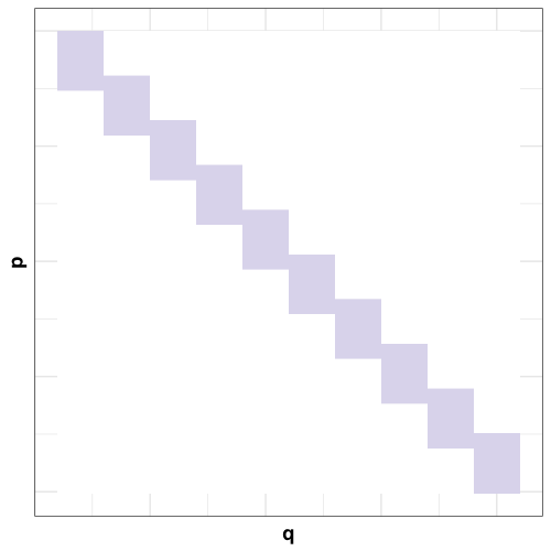
To assess the precision of the parameter estimates returned by the EM algorithm, we simulated data from two different data-generating truths: truly sparse and dense for the loadings . In both, the truth was set to factors. The dense loadings matrix has a grid of elements set uniformly between , whereas the truly sparse has a banded-diagonal structure with for the non-zero elements, as shown in Figure 2.
| Model | it | it | ||||||||
| Dense , | ||||||||||
| Flat | 10.0 | 10000.0 | 104.8 | 1173.3 | 2.0 | 10.0 | 15000.0 | 126.5 | 1895.7 | 2.0 |
| Normal-SS | 10.0 | 1859.7 | 92.4 | 1266.4 | 9.3 | 10.0 | 2461.0 | 112.5 | 1988.2 | 6.9 |
| MOM-SS | 10.0 | 1468.6 | 93.5 | 1294.3 | 9.7 | 10.0 | 2059.1 | 114.3 | 1998.5 | 6.3 |
| FastBFA | 9.6 | 976.9 | 137.9 | 1738.2 | 153.6 | 9.4 | 1400.4 | 163.2 | 5638.7 | 162.0 |
| LASSO-BIC | 10.0 | 5331.3 | 110.6 | 1682.5 | NA | 10.0 | 8607.7 | 137.4 | 2524.8 | NA |
| Dense , | ||||||||||
| Flat | 100.0 | 100000.0 | 313.2 | 1200.6 | 3.0 | 100.0 | 150000.0 | 376.2 | 1925.3 | 2.5 |
| Normal-SS | 34.8 | 3418.5 | 190.5 | 1190.7 | 4.2 | 14.8 | 5083.8 | 154.4 | 1911.8 | 4.0 |
| MOM-SS | 10.5 | 3215.9 | 108.9 | 1178.7 | 5.0 | 11.2 | 4232.8 | 135.6 | 1902.8 | 4.0 |
| FastBFA | 96.6 | 3379.3 | 297.4 | 451.2 | 11.3 | 97.3 | 4558.4 | 362.1 | 670.5 | 10.5 |
| LASSO-BIC | 11.0 | 4829.2 | 80.5 | 1682.7 | NA | 11.1 | 7839.6 | 99.5 | 2524.8 | NA |
| Sparse , | ||||||||||
| Flat | 10.0 | 10000.0 | 104.8 | 184.1 | 2.0 | 10.0 | 15000.0 | 126.4 | 301.4 | 2.0 |
| Normal-SS | 10.0 | 1300.1 | 55.8 | 124.1 | 3.9 | 10.0 | 1942.1 | 68.0 | 248.5 | 3.0 |
| MOM-SS | 10.0 | 1299.9 | 53.8 | 122.5 | 4.3 | 10.0 | 1943.0 | 69.4 | 235.2 | 2.3 |
| FastBFA | 8.7 | 1076.3 | 74.8 | 176.8 | 93.1 | 7.1 | 1320.4 | 84.7 | 344.2 | 122.7 |
| LASSO-BIC | 10.0 | 5304.3 | 77.4 | 424.0 | NA | 10.0 | 8397.0 | 93.3 | 636.3 | NA |
| Sparse , | ||||||||||
| Flat | 100.0 | 100000.0 | 313.7 | 310.8 | 3.0 | 100.0 | 150000.0 | 375.4 | 446.7 | 2.5 |
| Normal-SS | 22.0 | 2801.8 | 165.3 | 203.7 | 4.0 | 42.5 | 2795.9 | 230.0 | 335.1 | 4.3 |
| MOM-SS | 10.5 | 2156.8 | 109.7 | 194.1 | 5.0 | 11.2 | 2430.5 | 136.4 | 324.8 | 4.0 |
| FastBFA | 97.9 | 1508.9 | 283.0 | 215.2 | 9.9 | 97.6 | 2229.7 | 363.0 | 326.4 | 9.2 |
| LASSO-BIC | 10.0 | 4815.5 | 75.0 | 425.1 | NA | 10.0 | 7980.8 | 91.2 | 637.1 | NA |
We simulated observations from , with growing and , where the factors , the errors with , and the loadings are set as dense or sparse as in Figure 2. For comparison, FastBFA was initialised as our models via two-step least-squares (Section 4.3).
Table 1 shows the selected number of factors , the number of estimated non-zero loadings , the Frobenius norm (F.N.) between the true expected value and its reconstruction and between the true and reconstructed covariances , and the number of iterations until convergence. The mean across 100 different simulations is displayed and the model with smallest mean Frobenius norm per scenario is indicated in bold.
We first considered the unrealistic scenario where is dense and one guessed correctly the true number of factors . The aim of this setting was to investigate if MOM-SS shrinkage provided a poor estimation when the factors were not truly sparse. MOM-SS and Normal-SS performed similarly as grew, and competitively relative to the flat prior. To extend our example, we then set to illustrate the performance when there is sparsity in terms of the number of factors, but not within factors. LASSO-BIC had the best reconstruction for the mean but performed poorly on the covariance, whereas FastBFA outperformed all the models to estimate the covariance but performed poorly for the mean. However, MOM-SS had a good balance in terms of estimating the expected value and the covariance, being the second best in both cases.
We further illustrate our model under the arguably more interesting case of truly sparse loadings. First we set the true cardinality. In this scenario MOM-SS and Normal-SS presented the best results both for mean and covariance. This example reflects the advantages of shrinkage and the varimax rotation for the initialisation in the loadings, leading to good sparse solutions. Finally we considered the same scenario with . LASSO-BIC was best to estimate the mean at the cost of reduced precision in the covariance reconstruction. MOM-SS displayed the lowest error for the covariance and second smallest for the mean, showing a good balance between those metrics.
In general, MOM-SS achieved a good balance between estimating the mean, which is useful for dimensionality reduction, and sparse covariance estimation. Recall that we used a coordinate descent algorithm for the non-local prior, which as a potential drawback could require a larger number of iterations than performing jointly optimising multiple elements in . However, Table 1 showed that MOM-SS required roughly the same number of iterations to converge as the Normal-SS. We can see that MOM-SS and LASSO-BIC estimated accurately. Note that in general FastBFA had the highest estimated latent cardinality , due to the fat tails of the Laplace priors, which adds some columns of that contain very few non-zero loadings after the tenth factor, as shown in Supplementary Sections J and K. Nonetheless, this model displayed a mean number of non-zero loadings closer to the ground truth (1,300 and 1,940 for the and respectively under sparse ).


5.2 Batch effects
| Model | it | it | ||||||||
| Dense , | ||||||||||
| Flat | 10.0 | 2500.0 | 56.5 | 88.2 | 4.4 | 10.0 | 5000.0 | 71.9 | 120.2 | 4.0 |
| Normal-SS | 10.0 | 727.6 | 54.0 | 83.9 | 8.0 | 10.0 | 1398.7 | 68.6 | 116.5 | 4.5 |
| MOM-SS | 10.0 | 1097.3 | 55.1 | 84.6 | 15.2 | 10.0 | 1257.5 | 70.1 | 127.4 | 81.1 |
| ComBat-MLE | 10.0 | 2500.0 | 178.5 | 810.2 | 3.1 | 10.0 | 5000.0 | 249.2 | 1144.9 | 3.2 |
| FastBFA | 10.0 | 1153.0 | 89.0 | 834.5 | 12.3 | 10.0 | 2343.1 | 106.6 | 1182.6 | 10.9 |
| LASSO-BIC | 10.0 | 2109.9 | 99.2 | 833.1 | NA | 10.0 | 4377.1 | 118.1 | 1182.9 | NA |
| Dense , | ||||||||||
| Flat | 100.0 | 25000.0 | 140.7 | 157.6 | 5.0 | 100.0 | 50000.0 | 208.8 | 231.2 | 10.7 |
| Normal-SS | 29.7 | 983.5 | 87.4 | 111.2 | 6.3 | 10.0 | 2725.1 | 73.4 | 119.8 | 5.6 |
| MOM-SS | 10.0 | 1216.7 | 57.4 | 87.7 | 7.2 | 10.0 | 2293.5 | 74.0 | 120.4 | 6.3 |
| ComBat-MLE | 100.0 | 25000.0 | 70.6 | 822.6 | 33.8 | 100.0 | 50000.0 | 123.3 | 1161.0 | 14.8 |
| FastBFA | 35.3 | 1285.5 | 79.3 | 826.7 | 19.6 | 59.9 | 2589.0 | 126.8 | 1181.6 | 12.5 |
| LASSO-BIC | 12.9 | 1579.6 | 59.4 | 827.8 | NA | 11.1 | 2939.6 | 75.8 | 1171.2 | NA |
| Sparse , | ||||||||||
| Flat | 10.0 | 2500.0 | 49.7 | 68.5 | 4.1 | 10.0 | 5000.0 | 60.8 | 90.7 | 4.1 |
| Normal-SS | 10.0 | 330.0 | 45.7 | 58.7 | 4.9 | 10.0 | 650.0 | 55.9 | 77.0 | 4.1 |
| MOM-SS | 10.0 | 330.0 | 45.5 | 57.8 | 5.4 | 10.0 | 650.0 | 56.0 | 76.6 | 4.1 |
| ComBat-MLE | 10.0 | 2500.0 | 171.4 | 807.8 | 2.0 | 10.0 | 5000.0 | 244.5 | 1140.3 | 1.0 |
| FastBFA | 10.0 | 817.1 | 78.1 | 832.1 | 9.8 | 10.0 | 1617.5 | 104.2 | 1178.1 | 9.9 |
| LASSO-BIC | 10.0 | 2307.4 | 73.3 | 835.0 | NA | 10.0 | 4835.0 | 97.9 | 1181.1 | NA |
| Sparse , | ||||||||||
| Flat | 100.0 | 25000.0 | 140.4 | 146.4 | 5.0 | 100.0 | 50000.0 | 207.9 | 216.0 | 10.4 |
| Normal-SS | 93.2 | 372.9 | 139.9 | 143.7 | 7.2 | 10.0 | 2675.5 | 74.4 | 91.2 | 5.6 |
| MOM-SS | 10.0 | 1286.2 | 59.1 | 70.2 | 7.1 | 10.0 | 2197.0 | 75.6 | 92.8 | 6.3 |
| ComBat-MLE | 100.0 | 25000.0 | 70.8 | 821.1 | 42.6 | 100.0 | 50000.0 | 123.1 | 1157.3 | 14.3 |
| FastBFA | 41.5 | 976.5 | 84.8 | 828.2 | 18.1 | 65.8 | 1956.8 | 130.9 | 1179.8 | 13.7 |
| LASSO-BIC | 12.3 | 1663.3 | 56.0 | 824.7 | NA | 12.9 | 3794.4 | 70.2 | 1167.7 | NA |
We evaluate our method in our main setting of interest where there are mean and variance batch effects. We emphasise that, the competing methods are not designed to account for batch effects; thus, this is not a fair comparison but rather an illustration of how much inference can suffer when not properly accounting for batches. Also, since Flat-SS, Normal-SS and MOM-SS do incorporate batches, comparing them illustrates the advantages of NLP-based sparsity, e.g. see the bottom row in Figure 4.
We simulated data with a mean and variance batch effect, , sample size and growing or . We set , and batches and considered the truly sparse and dense loadings in Figure 2. Factors were drawn from , errors from , where and for ; from a continuous Uniform(0,3) and from a discrete Uniform{0,1}. We set the first values of to -2 and the other to 2 and , for we fixed to 2 for the first batch and 0 for the second. We compared our models with FastBFA and LASSO-BIC without batch effect correction for illustration of the importance of a proper mean and variance batch effect adjustment; and with empirical Bayes batch effect correction, ComBat, followed with an MLE estimation of the parameters ComBat-MLE. Table 2 shows the results. The following plots show the comparison between the true against their reconstruction in the scenario with sparsity with factors .
Firstly, we considered the scenario when one correctly guesses and loadings are truly dense and sparse solutions could provide poor estimations. MOM-SS and Normal-SS achieved similar performance as the case without batch effect and similar results were observed for the case. MOM-SS estimated correctly the latent cardinality and achieved a small estimation error for .
Secondly, we studied the scenario with sparse factors. MOM-SS achieved a small estimation error for the mean and was effective in estimating . LASSO-BIC had a small estimation error of the mean, although solutions were generally less sparse in the number of non-zero loadings.
It is important to highlight that even though ComBat-MLE, FastBFA and LASSO-BIC achieved a precise reconstruction of for purposes of dimensionality reduction the estimates of are less precise as shown in Table 2 and Figure 4 (right panels). Furthermore, the estimated covariance of the model displayed in the heatmap in Supplementary Sections L and M, Supplementary Figures 10 (j)-(l) and 12 (j)-(l) are nowhere close to the generating truth. We remark that for FastBFA and LASSO-BIC these results mainly highlight that one should take into account batch effects. For Combat-MLE they highlight the limitations of using two-step procedures relative to a joint estimation of the factor model and batch effects


5.3 Applications to cancer datasets
We applied our method to two high-dimensional cancer datasets, related to ovarian and lung cancer. For the ovarian cancer we combined information from two datasets from the package curatedOvarianData 1.16.0. The first was the Illumina Human microRNA array expression dataset E.MTAB.386, formed by Angiogenic mRNA and microRNA gene expression signature with patients (Bentink et al. 2012). The second was the NCI-60 GEO dataset GSE30161 and consisted of multi-gene expression predictors of single drug responses to adjuvant chemotherapy in ovarian carcinoma for patients (Ferriss et al. 2012). For the lung cancer, we used microarray and mRNA-array, data from two different high-throughput platforms: Affymetrix Human Genome U133A 2.0 Array with patients and Affymetrix Human Exon 1.0 ST Array with (Wan et al. 2016).
We considered two main tasks: to give a visual representation of the latent factors of the data, i.e. an unsupervised dimension reduction task and a supervised survival analysis using the factors obtained in our method as predictions. Prior to our analyses, we selected the 10% genes with highest total variance across all samples obtaining for ovarian and for lung. All data sets have been normalised to zero mean and unit variance. We included the age at initial pathologic diagnosis as a covariate.
5.3.1 Unsupervised: Data visualisation
Our first goal was to demonstrate the usefulness of our method as a data visualisation tool. We remark that there are no other model-based approaches to jointly adjust for batch effects and estimate latent factors. Thus, for comparison we first corrected the data using ComBat and then estimated the latent parameters via MLE and FastBFA akin to Section 5.2. To decide the number of factors for ComBat-MLE, we carried a principal component analysis to the corrected data prior to factor analysis and chose a number of components that explained 90% or 70% of the total variance. It is important to notice that we are doing an over-optimistic assessment of ComBat-MLE and ComBat-FastBFA as we are doing a cross-validated factor analysis over the ComBat-corrected data, as opposed to also running ComBat in an out-of-sample fashion.


Figure 5 illustrates the advantages of our method. We can clearly see the usefulness of ComBat correction (middle panels) compared to scenarios without correction (top panels), ComBat removes systematic differences in location and scale across the 2 batches. Nonetheless, the latent coordinates displayed distinct covariances for the ovarian cancer dataset. Such covariances were not presented in the MOM-SS latent factors (bottom panels). Figures 5 (g) and (h) show the two factors that contribute the most to the covariance, i.e. the ones with highest . The latent coordinates were post-processed to standardised their variance as explained in Section 4.4.
5.3.2 Supervised: Survival analysis
We also illustrate the potential of our method as a surpervised tool, performing a survival analysis that aims to predict the time until death. To do that, we applied a Cox proportional hazards model (Cox 1972) using as covariates the latent coordinates obtained in our models. We used the coxph function of the R package survival 2.38 (Therneau 2015). We then used the concordance index to asses the quality of our predictions. This index is a non-parametric metric to quantify the power of a prediction rule via a pair-wise comparison that measures the probability of concordance between the predicted and the observed survival time (Harrell Jr. et al. 1982). To obtain the concordance index we used the function concordance.index in the R package survcomp (Schröeder et al. 2011). The presented results are from 10 independent runs of 10-fold cross-validation. We initialised MOM-SS with the values obtained for the Flat model along with the other initialisations discussed in Section 4.3 and chose the one with smallest leave-one-out cross-validated concordance index.
For the cancer data sets, Table 3 shows that Flat-SS achieved a high concordance index, even though loadings are not sparse. Normal-SS gave sparse loading representations but displayed a concordance index lower than Flat-SS; this illustrates a lack of power to detect truly non-zero loadings. In general, MOM-SS provided sparse loadings and a good concordance index. In the ovarian cancer data, MOM-SS achieved a concordance index similar to ComBat-MLE 90% with considerably less factors (4 instead of 101) and a bit higher than Normal-SS. In the lung cancer data MOM-SS achieved a high concordance index, particularly relative to Normal-SS and ComBat-MLE 70%. The competing methods generally lead to less sparse solutions and their performance fluctuates across scenarios. In the lung cancer data ComBat-MLE, despite its good performance, had a concordance index that proved to be sensitive to the number of factors (see ComBat-MLE 90% vs 70%). ComBat-FastBFA provided competitive results with a non-sparse reconstruction, recovering values in the latent loadings that were close to zero (even though not exactly zero) and smaller than the ones of the Flat-SS. MOM-SS proved to have practical advantages as a supervised tool in comparison with the two-step approaches considered here. Overall, MOM-SS provided a more stable performance that achieved a good balance between sparsity and prediction accuracy.
| Ovarian | Lung | |||||
|---|---|---|---|---|---|---|
| Concordance index | Concordance index | |||||
| Flat | 100.0 | 100700.0 | 0.634 | 100.0 | 119800.0 | 0.669 |
| Normal-SS | 7.8 | 7854.6 | 0.568 | 11.0 | 13178.0 | 0.489 |
| MOM-SS | 4.0 | 4028.0 | 0.588 | 74.0 | 88652.0 | 0.665 |
| ComBat-MLE 90% | 101.0 | 101707.0 | 0.589 | 79.0 | 94642.0 | 0.688 |
| ComBat-MLE 70% | 41.0 | 41287.0 | 0.588 | 30.0 | 35940.0 | 0.568 |
| ComBat-FastBFA | 100.0 | 100700.0 | 0.527 | 100.0 | 119800.0 | 0.707 |
6 Discussion
We have presented a novel model to integrate data from multiple sources using joint dimension reduction and batch effect adjustment via high-dimensional latent factor regression.We outlined three different prior configurations for the loadings and Laplace-tailed extensions whose deeper analysis remain as future work. To our knowledge this is the first time NLPs are implemented in the factor analysis context. We gave novel EM algorithms to obtain posterior modes. We showed that the use of sparse models increases the quality of our estimations even in the absence of batches. In our empirical results MOM-SS priors proved to be appealing, improving the estimation of factor cardinality and encouraging parsimony and selective shrinkage.
We illustrated the utility of our method in unsupervised and supervised frameworks. MOM-SS provided dimension reduction that corrected distinct covariance patterns present in two-stage methods that adjust variances separately from fitting the factor model. Such patterns are highly likely to be technical artefacts, since patients from different batches are believed to be exchangeable. Our model demonstrated to be useful for downstream analyses, achieving a competitive concordance indexes, in some cases with substantially less factors. It is important to notice that although our examples focus on gene expression of cancer datasets, the applications should also be useful in other settings.
We also remark that our novel MOM-SS and its closed-form EM updates can be extended to frameworks of interest beyond factor models such as: linear regression, generalised linear models as well as graphical models.
Our model assumes common factors across the datasets being integrated. An interesting extension for future research is to consider more complex settings where some of the factors differ across data sources or where one wishes to integrate datasets by adding variables (as opposed to adding individuals as we did here), or where potentially same variables were only recorded for a subset of the individuals.
Supplementary Materials
The supplementary materials are as follow: EM algorithm under a flat, Normal-SS, MOM-SS, Laplace-SS and Laplace-MOM-SS on the loadings, a pseudo-code-algorithm for the weighted 10-fold cross-validation, and heatmaps for , and for the different simulated scenarios and setting .
Acknowledgements
We thank Chris Yau for valuable insights and Veronika Ročková for providing the FastBFA package.
Funding
Alejandra Avalos-Pacheco gratefully acknowledges the Mexican National Council of Science and Technology (CONACYT) grant no. CVU5464444. David Rossell was partially funded by the NIH grant R01 CA158113-01, RyC-2015-18544 and Ayudas Fundación BBVA a equipos de investigación científica 2017.
APPENDIX
Appendix A Proof of Lemma 1, MOM-SS global mode
Proof.
Our goal is to max . Take derivative with respect to
Roots are and .
If then the global max is , else the global max is . After trivial algebra, .
For ease of notation let . Note that and that, since , , that implies that . Then if and only if . Equivalently, if and only if .
- •
Suppose . Then left-hand side is , and right-hand side is . Hence global maximum is
- •
Suppose . Then left-hand side is , and right-hand side is . Hence global maximum is ∎
Appendix B Proof of Lemma 2, Laplace-SS global mode.
Proof.
Our purpose is to find the maximum of , where , and . Setting , we obtain
- •
For , we look for the solutions of . Note and . Thus
- •
For , we look for the solutions of . Thus
Appendix C Proof of Lemma 3, Laplace-MOM-SS global mode
Proof.
We aim to find the maximum of , where , and . Note that when , . Thus, the maximum of is one of its critical points. Setting , we obtain
- •
For , we look for the solutions of .
The roots of this polynomial are . Note that since and . Hence, the only acceptable root is , as the other one is negative.
- •
For , we look for the solutions of .
The roots of this polynomial are . As before, . Hence, the only acceptable root is , as the other one is positive.
- •
Suppose . Then clearly for all , i.e. the function is even. Therefore, and are opposite and both arg maxima.
- •
Suppose . By definition of , for all . In particular, and .
- •
Suppose . Then for all . In particular, and . ∎
References
- Alter et al. (2000) Alter, O., Brown, P. O., and Botstein, D. (2000). Singular value decomposition for genome-wide expression data processing and modeling. Proceedings of the National Academy of Sciences 97(18), 10101–10106.
- Avio et al. (2015) Avio, C. G., Gorbi, S., Milan, M., Benedetti, M., Fattorini, D., d’Errico, G., Pauletto, M., Bargelloni, L., and Regoli, F. (2015). Pollutants bioavailability and toxicological risk from microplastics to marine mussels. Environmental Pollution 198, 211 – 222.
- Bar et al. (2018) Bar, H., Booth, J., and Wells, M. T. (2018). A scalable empirical Bayes approach to variable selection in generalized linear models. arXiv:1803.09735, 1–20.
- Benito et al. (2004) Benito, M., Parker, J., Du, Q., Wu, J., Xiang, D., Perou, C. M., and Marron, J. S. (2004). Adjustment of systematic microarray data biases. Bioinformatics 20(1), 105–114.
- Bentink et al. (2012) Bentink, S., Haibe-Kains, B., Risch, T., Fan, J.-B., Hirsch, M. S., Holton, K., Rubio, R., April, C., Chen, J., Wickham-Garcia, E., Liu, J., Culhane, A., Drapkin, R., Quackenbush, J., and Matulonis, U. A. (2012, 02). Angiogenic mRNA and microRNA gene expression signature predicts a novel subtype of serous ovarian cancer. PLOS ONE 7(2), 1–9.
- Bersanelli et al. (2016) Bersanelli, M., Mosca, E., Remondini, D., Giampieri, E., Sala, C., Castellani, G., and Milanesi, L. (2016). Methods for the integration of multi-omics data: mathematical aspects. BMC Bioinformatics 17(2), 167–177.
- Burges (2010) Burges, C. J. C. (2010). Dimension reduction: A guided tour. Foundations and Trends in Machine Learning 2(4), 276–365.
- Carvalho et al. (2009) Carvalho, C., Polson, N., and Scott, J. (2009). Handling sparsity via the horseshoe. Journal of Machine Learning Research 5, 73–80.
- Carvalho et al. (2008) Carvalho, C. M., Chang, J., Lucas, J. E., Nevins, J. R., Wang, Q., and West, M. (2008). High-dimensional sparse factor modeling: Applications in gene expression genomics. Journal of the American Statistical Association 103(484), 1438–1456.
- Cox (1972) Cox, D. R. (1972). Regression models and life-tables. Journal of the Royal Statistical Society, Series B: Methodological 34, 187–220.
- Cunningham and Ghahramani (2015) Cunningham, J. P. and Ghahramani, Z. (2015). Linear dimensionality reduction: Survey, insights, and generalizations. Journal of Machine Learning Research 16, 2859–2900.
- De Vito et al. (2018a) De Vito, R., Bellio, R., Trippa, L., and Parmigiani, G. (2018a). Bayesian multi-study factor analysis for high-throughput biological data. arXiv:1806.09896, 1–35.
- De Vito et al. (2018b) De Vito, R., Bellio, R., Trippa, L., and Parmigiani, G. (2018b). Multi-study factor analysis. arXiv:1611.06350, 1–26.
- Dempster et al. (1977) Dempster, A. P., Laird, N. M., and Rubin, D. B. (1977). Maximum likelihood from incomplete data via the EM algorithm. Journal of the Royal Satistical Society, Series B: Statistical Methodology 39(1), 1–38.
- Dunson and Bhattacharya (2011) Dunson, D. and Bhattacharya, A. (2011). Sparse Bayesian infinite factor models. Biometrika 98, 291–306.
- Ferriss et al. (2012) Ferriss, J. S., Kim, Y., Duska, L., Birrer, M., Levine, D. A., Moskaluk, C., Theodorescu, D., and Lee, J. K. (2012, 02). Multi-gene expression predictors of single drug responses to adjuvant chemotherapy in ovarian carcinoma: Predicting platinum resistance. PLOS ONE 7(2), 1–9.
- Fortin et al. (2016) Fortin, J.-P., Sweeney, E. M., Muschelli, J., Crainiceanu, C. M., and Shinohara, R. T. (2016). Removing inter-subject technical variability in magnetic resonance imaging studies. NeuroImage 132, 198–212.
- Fox and Dunson (2015) Fox, E. B. and Dunson, D. B. (2015). Bayesian nonparametric covariance regression. Journal of Machine Learning Research 16, 2501–2542.
- Frühwirth-Schnatter and Lopes (2018) Frühwirth-Schnatter, S. and Lopes, H. F. (2018). Sparse Bayesian factor analysis when the number of factors is unknown. arXiv:1804.04231, 1–34.
- Fúquene et al. (2018) Fúquene, J., Steel, M., and Rossell, D. (2018). On choosing mixture components via non-local priors. arXiv:1604.00314, 1–72.
- Ganzfried et al. (2013) Ganzfried, B. F., Riester, M., Haibe-Kains, B., Risch, T., Tyekucheva, S., Jazic, I., Wang, X. V., Ahmadifar, M., Birrer, M., Parmigiani, G., Huttenhower, C., and Waldron, L. (2013). curatedovariandata: Clinically annotated data for the ovarian cancer transcriptome. Database 2013.
- George and McCulloch (1993) George, E. and McCulloch, R. (1993). Variable selection via Gibbs sampling. Journal of the American Statistical Association 88(423), 881–889.
- George and McCulloch (1997) George, E. and McCulloch, R. (1997). Approaches for Bayesian variable selection. Statistica Sinica, 339–374.
- Ghahramani and Beal (2000) Ghahramani, Z. and Beal, M. J. (2000). Variational inference for Bayesian mixtures of factor analysers. In S. A. Solla, T. K. Leen, and K. Müller (Eds.), Advances in Neural Information Processing Systems 12, 449–455. MIT Press.
- Goh et al. (2017) Goh, W. W. B., Wang, W., and Wong, L. (2017). Why batch effects matter in omics data, and how to avoid them. Trends in Biotechnology 35, 498–507.
- Griffiths and Ghahramani (2011) Griffiths, T. L. and Ghahramani, Z. (2011, July). The Indian Buffet Process: An introduction and review. J. Mach. Learn. Res. 12, 1185–1224.
- Harrell Jr. et al. (1982) Harrell Jr., F. E., Califf, R. M., Pryor, D. B., Lee, K. L., and Rosati, R. A. (1982). Evaluating the yield of medical tests. JAMA 247(18), 2543–2546.
- Hastie et al. (2001) Hastie, T., Tibshirani, R., and Friedman, J. (2001). The Elements of Statistical Learning. Springer Series in Statistics. New York, NY, USA: Springer New York Inc.
- Hirose and Yamamoto (2015) Hirose, K. and Yamamoto, M. (2015, Sep). Sparse estimation via nonconcave penalized likelihood in factor analysis model. Statistics and Computing 25(5), 863–875.
- Hirose et al. (2016) Hirose, K., Yamamoto, M., and Nagata, H. (2016). fanc: Penalized Likelihood Factor Analysis via Nonconvex Penalty. R package version 2.2.
- Hoff and Niu (2012) Hoff, P. and Niu, X. (2012). A covariance regression model. Statistica Sinica 22, 729–753.
- Hornung et al. (2016) Hornung, R., Boulesteix, A.-L., and Causeur, D. (2016). Combining location-and-scale batch effect adjustment with data cleaning by latent factor adjustment. BMC Bioinformatics 17(1), 1–19.
- Johnson and Wichern (1988) Johnson, R. A. and Wichern, D. W. (Eds.) (1988). Applied Multivariate Statistical Analysis. Upper Saddle River, NJ, USA: Prentice-Hall, Inc.
- Johnson and Rossell (2010) Johnson, V. E. and Rossell, D. (2010). On the use of non-local prior densities in Bayesian hypothesis tests. Journal of the Royal Statistical Society Series B: Statistical Methodology 72(2), 143–170.
- Johnson and Rossell (2012) Johnson, V. E. and Rossell, D. (2012). Bayesian model selection in high-dimensional settings. Journal of the American Statistical Association 107(498), 649–660.
- Johnson and Li (2009) Johnson, W. E. and Li, C. (2009). Adjusting Batch Effects in Microarray Experiments with Small Sample Size Using Empirical Bayes Methods, 113–129. John Wiley & Sons, Ltd.
- Johnson et al. (2007) Johnson, W. E., Li, C., and Rabinovic, A. (2007). Adjusting batch effects in microarray expression data using empirical Bayes methods. Biostatistics (Oxford, England) 8(1), 118–27.
- Kaiser (1958) Kaiser, H. F. (1958, Sep). The varimax criterion for analytic rotation in factor analysis. Psychometrika 23(3), 187–200.
- Knowles and Ghahramani (2011) Knowles, D. A. and Ghahramani, Z. (2011). Nonparametric Bayesian sparse factor models with application to gene expression modeling. The Annals of Applied Statistics 5(2B), 1534–1552.
- Leek et al. (2017) Leek, J. T., Johnson, W. E., Parker, H. S., Fertig, E. J., Jaffe, A. E., Storey, J. D., Zhang, Y., and Torres, L. C. (2017). sva: Surrogate Variable Analysis. R package version 3.26.0.
- Leek et al. (2010) Leek, J. T., Scharpf, R. B., Bravo, H. C., Simcha, D., Langmead, B., Johnson, W. E., Geman, D., Baggerly, K., and Irizarry, R. A. (2010, October). Tackling the widespread and critical impact of batch effects in high-throughput data. Nat Rev Genet 11(10), 733–739.
- Leek and Storey (2007) Leek, J. T. and Storey, J. D. (2007, 09). Capturing heterogeneity in gene expression studies by surrogate variable analysis. PLoS Genet 3(9), 1–12.
- Lopes and West (2004) Lopes, H. F. and West, M. (2004). Bayesian model assessment in factor analysis. Statistica Sinica 14, 41–67.
- Lucas et al. (2006) Lucas, J., Carvalho, C., Wang, Q., Bild, A., Nevins, J., and West, M. (2006). Sparse statistical modelling in gene expression genomics. In Bayesian Inference for Gene Expression and Proteomics, 155–176. Cambridge University Press.
- Mitchell and Beauchamp (1988) Mitchell, T. J. and Beauchamp, J. J. (1988). Bayesian variable selection in linear regression. Journal of the American Statistical Association 83(404), 1023–1032.
- Olivetti et al. (2012) Olivetti, E., Greiner, S., and Greiner, S. (2012). ADHD diagnosis from multiple data sources with batch effects. Frontiers in Systems Neuroscience 6, 1662–5137.
- Parker et al. (2014) Parker, H. S., Corrada Bravo, H., and Leek, J. T. (2014, September). Removing batch effects for prediction problems with frozen surrogate variable analysis. PeerJ 2, e561.
- Rhodes et al. (2004) Rhodes, D. R., Yu, J., Shanker, K., Deshpande, N., Varambally, R., Ghosh, D., Barrette, T., Pandey, A., and Chinnaiyan, A. M. (2004). Large-scale meta-analysis of cancer microarray data identifies common transcriptional profiles of neoplastic transformation and progression. Proceedings of the National Academy of Sciences of the United States of America 101(25), 9309–9314.
- Rossell and Telesca (2017) Rossell, D. and Telesca, D. (2017). Nonlocal priors for high-dimensional estimation. Journal of the American Statistical Association 112(517), 254–265.
- Ročková and George (2014) Ročková, V. and George, E. I. (2014). EMVS: The EM approach to Bayesian variable selection. Journal of the American Statistical Association 109(506), 828–846.
- Ročková and George (2017) Ročková, V. and George, E. I. (2017). Fast Bayesian factor analysis via automatic rotations to sparsity. Journal of the American Statistical Association 111(516), 1608–1622.
- Ročková and George (2018) Ročková, V. and George, E. I. (2018). The Spike-and-Slab LASSO. Journal of the American Statistical Association 113(521), 431–444.
- Schadt et al. (2001) Schadt, E. E., Li, C., Ellis, B., and Wong, W. H. (2001). Feature extraction and normalization algorithms for high-density oligonucleotide gene expression array data. Journal of Cellular Biochemistry 84(S37), 120–125.
- Scherer (2009) Scherer, A. (2009). Batch Effects and Noise in Microarray Experiments: Sources and Solutions. Wiley Series in Probability and Statistics. Wiley.
- Schröeder et al. (2011) Schröeder, M. S., Culhane, A., Quackenbush, J., and Haibe-Kains, B. (2011). survcomp: an R/Bioconductor package for performance assessment and comparison of survival models. Bioinformatics 27(22), 3206–3208.
- Schwarz (1978) Schwarz, G. (1978, 03). Estimating the dimension of a model. Ann. Statist. 6(2), 461–464.
- Seber (1984) Seber, G. (1984). Multivariate observations. Wiley series in probability and mathematical statistics. New York, NY: Wiley.
- Shah et al. (2011) Shah, M., Xiao, Y., Subbanna, N., Francis, S., Arnold, D. L., Collins, D. L., and Arbel, T. (2011). Evaluating intensity normalization on MRIs of human brain with multiple sclerosis. Medical Image Analysis 15(2), 267 – 282.
- Shi et al. (2019) Shi, G., Lim, C. Y., and Maiti, T. (2019). Model selection using mass-nonlocal prior. Statistics & Probability Letters 147(C), 36–44.
- Shinohara et al. (2014) Shinohara, R. T., Sweeney, E. M., Goldsmith, J., Shiee, N., Mateen, F. J., Calabresi, P. A., Jarso, S., Pham, D. L., Reich, D. S., and Crainiceanu, C. M. (2014). Statistical normalization techniques for magnetic resonance imaging. NeuroImage : Clinical 6, 9–19.
- Therneau (2015) Therneau, T. M. (2015). A Package for Survival Analysis in S. version 2.38.
- Wan et al. (2015) Wan, Y.-W., Allen, G. I., Anderson, M. L., and Liu, Z. (2015). TCGA2STAT: Simple TCGA Data Access for Integrated Statistical Analysis in R. R package version 1.2.
- Wan et al. (2016) Wan, Y.-W., Allen, G. I., and Liu, Z. (2016). TCGA2STAT: simple TCGA data access for integrated statistical analysis in R. Bioinformatics 32(6), 952–954.
- Wang and Zhao (2015) Wang, J. and Zhao, Q. (2015). cate: High Dimensional Factor Analysis and Confounder Adjusted Testing and Estimation. R package version 1.0.4.
- West (2003) West, M. (2003). Bayesian factor regression models in the “large p, small n” paradigm. In Bayesian Statistics 7, 723–732. Oxford University Press.
- Witten et al. (2009) Witten, D. M., Tibshirani, R., and Hastie, T. (2009). A penalized matrix decomposition, with applications to sparse principal components and canonical correlation analysis. Biostatistics 10(3), 515–534.
- Yang et al. (2002) Yang, Y. H., Dudoit, S., Luu, P., Lin, D. M., Peng, V., Ngai, J., and Speed, T. P. (2002). Normalization for cDNA microarray data: a robust composite method addressing single and multiple slide systematic variation. Nucleic Acids Research 30(4), e15.
SUPPLEMENTARY MATERIAL
Appendix D EM algorithm under a flat prior on the loadings
Here, we outline the derivation of the Expectation-Maximisation (EM) algorithm to fit the latent factor regression model with mean and variance adjustment presented in Section 4.1 via Maximum a posteriori (MAP) estimation. Our goal is to find values that maximise the log-posterior
| (34) |
To maximise (34) the EM algorithm make use of complete-data log-posterior associated to
| (35) |
For simplicity we will denote by the probability with respect to the latent variables and conditioning upon at time t. Similarly, the mean conditional on and all other model parameters , and likewise for .
We first outline the E-step, which is based on taking the expectation of Expression (35) with respect to , namely:
| (36) |
where is a constant, and we have defined as usual diag and to be the unique such that .
Expression (36) only depends on through the conditional posterior mean
| (37) |
and the conditional second moments
| (38) |
The M-step consists in maximising Equation (36) with respect to . To this end, we set its partial derivatives to 0, as shown below.
| (39) |
Maximisation of for a fixed batch is obtained by taking the derivative with respect to
| (41) |
To maximise with respect to we set
| (43) |
Taking the row of matrix and solving Equation (43):
| (44) |
Equation (44) has the form of a ridge regression estimator with penalty , inducing an equal shrinkage to each coefficient of
Appendix E EM algorithm under Normal-SS
Akin to the Flat prior, we first take the expectation of the complete-data log-posterior with respect to the latent variables and conditioning upon the current :
| (45) |
Due to the conjugate Normal-SS hierarchical construction, Expression (45) can be split in order to simplify the EM algorithm as , where:
| (46) | ||||
| (47) |
The E-step for resembles the one for the flat prior model shown in Supplement D, plus an extra conditional expectation:
with given by
The first and second moments and respectively are given in Supplement D.
For corresponds to a beta-binomial prior on , with conditional expectations .
In the M-step we proceed by optimising and independently, in 2 steps: a maximisation of with respect to , and , followed by a maximisation of with respect to . Setting to 0 the partial derivative with respect to gives:
| (48) |
with , and being the Hadamard (element-wise) product of two matrices and . Taking the row of matrix and solving equation (48) we obtain:
for Updates for and are the same ones given in Supplement D.
Finally,
| (49) |
Solving Equation (49) and substituting :
| (50) |
Appendix F EM algorithm under MOM-SS
Analogous to Normal-SS, we first take the expected complete-data log-posterior . By construction is of the same form than in Equation (47) and is given by
| (51) |
For the E-step and are the same as the ones in Supplement D for the flat prior. The new conditional expectation for the inclusion probability is
and .
For the M-step of the loadings, we consider using a coordinate descent algorithm (CDA) that leads to closed-form expressions for . The partial derivative of (51) is:
| (52) |
with , , a matrix with elements and being the Hadamard (element-wise) product of two matrices and .
Define and . The global maximum is if or if . See Appendix A for details.
Finally, the updates for , and are equivalent to the ones obtained for Normal-SS.
Appendix G EM algorithm under Laplace-SS
Now, the part of the expected complete-data log-posterior for the Laplace-SS is
| (54) |
In the conditional expectations is
and with for .
The M-step update for is obtain by setting to 0 the partial derivative with respect to , for
| (55) |
with with element : .
Taking the partial derivative of (54) with respect to , when and setting it to 0 we obtain:
| (56) |
for .
Define and .
If , then . If , then . If , then . See Appendix B for details.
Appendix H EM algorithm under Laplace-MOM-SS
Finally, for Laplace-MOM-SS is given by:
| (57) |
The new conditional expectation for the inclusion probability is
and .
For the M-step of the loadings, we consider using a coordinate descent algorithm (CDA) that performs successive univariate optimisation with respect to each .
Notice that when , the value of , thus the solution for the optimisation is given by setting .
The partial derivative of (57) w.r.t. is
| (58) |
with with element : , a matrix with elements and being the Hadamard (element-wise) product of two matrices and .
Taking the partial derivative of (57) with respect to , when and setting it to 0 we obtain:
| (59) |
for .
Define and .
If , then . If , then . If , then or . See Appendix C for details.
Appendix I Weighted 10-fold cross-validation
We aim to a pseudo-code-algorithm for the weighted 10-fold cross-validation used through this paper.
set 10 random cross-validation subsets of
| Observations: | |
|---|---|
| Covariates: | |
| Batches: |
for do
and
| input: | |
|---|---|
| output: |
set: Test factors
compute end for
Appendix J Plots simulations of truly sparse loadings scenario and no batch effect
The following plots present the heatmaps of the reconstruction of and for the scenario with truly sparse loadings , setting and without batch effects.


Appendix K Plots simulations dense loadings and no batch effect
The following plots show the heatmaps of the reconstruction of and for the scenario with dense loadings , setting and without batch effects.


Appendix L Plots simulations truly sparse loadings and batch effect
Visual representation of the reconstruction of and for the scenario with truly sparse loadings , setting and with mean and variance batch effects.


Normal


ComBat

FastBFA

LASSO


Appendix M Plots simulations dense loadings and batch effect
Graphical representation of the reconstruction of and for the scenario with dense loadings , setting and with mean and variance batch effects.


Normal


ComBat

FastBFA

LASSO


