跳到论文正文
W Papers独立论文阅读器 arXiv:1810.09633 论文正文 计算阅读时间 · 0%
引用这篇论文根据当前论文元数据生成,正式投稿前建议核对。


License: arXiv.org perpetual non-exclusive license
arXiv:1810.09633v2 [cs.FL] 11 Jul 2019

Moore-Machine Filtering for
Timed and Untimed Pattern Matching

Masaki Waga    Ichiro Hasuo Thanks: This article was presented in the International Conference on Embedded Software 2018 and appears as part of the ESWEEK-TCAD special issue. Thanks: This work is supported by JST ERATO HASUO Metamathematics for Systems Design Project (No. JPMJER1603), and JSPS Grants-in-Aid No. 15KT0012 & 18J22498. Thanks: M. Waga and I. Hasuo are with National Institute of Informatics, Tokyo, Japan, and SOKENDAI (the Graduate University for Advanced Studies), Kanagawa, Japan. Thanks: M. Waga is a JSPS Research Fellow.
Abstract

Monitoring is an important body of techniques in runtime verification of real-time, embedded and cyber-physical systems. Mathematically, the monitoring problem can be formalized as a pattern matching problem against a pattern automaton. Motivated by the needs in embedded applications—especially the limited channel capacity between a sensor unit and a processor that monitors—we pursue the idea of filtering as preprocessing for monitoring. Technically, for a given pattern automaton, we present a construction of a Moore machine that works as a filter. The construction is automata-theoretic, and we find the use of Moore machines particularly suited for embedded applications, not only because their sequential operation is relatively cheap but also because they are amenable to hardware acceleration by dedicated circuits. We prove soundness (i.e. absence of lost matches), too. We work in two settings: in the untimed one, a pattern is an NFA; in the timed one, a pattern is a timed automaton. The extension of our untimed construction to the timed setting is technically involved, but our experiments demonstrate its practical benefits.

Index Terms: 
Monitoring, filtering, timed pattern matching, Moore machine, timed automaton, real-time system
©2018 IEEE. DOI: 10.1109/TCAD.2018.2857358

I Introduction

I-A Monitoring and (Timed) Pattern Matching

The complexity of cyber-physical systems (CPS) has been rapidly growing, due to increasingly advanced digital control that realizes not only enhanced efficiency (e.g. in cars’ fuel consumption) but also totally new functionalities such as automatic driving. Getting those systems right is, therefore, a problem that is as important, and as challenging, as ever.

Due to such complexity of CPS, combined with other reasons such as black-box components provided by other suppliers, formal verification in the conventional sense is often hard to apply to real-world CPS. This has made researchers and practitioners turn to so-called lightweight formal methods. Runtime verification is a major branch therein, where execution traces of a given system is checked against a given specification [1]. Various algorithms for monitoring have been proposed for this purpose.

Mathematically speaking, one common formalization of the monitoring problem is as the problem of pattern matching.11 1 Another common formalization is as what we call the pattern search problem. Pattern search is easier than pattern matching, but is less informative. Their comparison is at the end of §I. In case an execution trace is given by a word w=a1​a2​…​anw=a_{1}a_{2}\dotsc a_{n}, the expected outcome is the set

Match⁡(w,𝗉𝖺𝗍):={(i,j)∣w|[i,j]⊧𝗉𝖺𝗍}(where w|[i,j]=ai​ai+1​…​aj)\begin{array}[]{r}\mathrm{Match}(w,\mathsf{pat})\;:=\;\{(i,j)\mid w|_{[i,j]}\models\mathsf{pat}\}\\ \qquad\text{(where $w|_{[i,j]}=a_{i}a_{i+1}\dotsc a_{j}$)}\end{array} (1)

of pairs (i,j)(i,j) of indices, the restriction of ww to which satisfies the given pattern 𝗉𝖺𝗍\mathsf{pat}. The pattern 𝗉𝖺𝗍\mathsf{pat} can be given by a string, a set of strings, a regular expression, an automaton, etc.

Example I.1.

Consider a word w1=𝚊𝚋𝚋​𝚋𝚋𝚋​𝚊𝚊𝚋w_{1}=\mathtt{abb\,bbb\,aab} and a pattern given by a regular expression 𝒜1=𝚊𝚊∗​b\mathcal{A}_{1}=\mathtt{aa}^{*}b. There are three matches, and we have Match⁡(w1,𝒜1)={(1,2),(7,9),(8,9)}\mathrm{Match}(w_{1},\mathcal{A}_{1})=\{(1,2),(7,9),(8,9)\}.

More interesting in the CPS context is the timed version of pattern matching. In one common formalization, an execution trace is given by a timed word—a sequence of time-stamped characters such as w2=(𝚊,0.1)​(𝚋,2.5)​(𝚊,3.5)​(𝚋,4.8)w_{2}=(\mathtt{a},0.1)(\mathtt{b},2.5)(\mathtt{a},3.5)(\mathtt{b},4.8). A pattern 𝗉𝖺𝗍\mathsf{pat} is then specified by a timed automaton (TA) 𝒜\mathcal{A} from [2], and we compute the set

Match⁡(w,𝒜):={(t,t′)∈ℝ≥02|t<t′​ and ​w|(t,t′)∈L⁡(𝒜)}\mathrm{Match}(w,\mathcal{A})\;:=\;\bigl\{\,(t,t^{\prime})\in{\mathbb{R}}_{\geq 0}^{2}\;\big|\;t<t^{\prime}\text{ and }w|_{(t,t^{\prime})}\in L(\mathcal{A})\,\bigr\} (2)

of intervals (t,t′)(t,t^{\prime}), the restriction of ww to which is accepted by the TA 𝒜\mathcal{A}. Unlike the untimed setting, a TA 𝒜\mathcal{A} allows one to express various real-time constraints, which leads to a much more refined analysis of execution traces of CPS.

Example I.2.

Consider the timed word w2=(𝚊,0.1)​(𝚋,2.5)​(𝚊,3.5)​(𝚋,4.8)w_{2}=(\mathtt{a},0.1)(\mathtt{b},2.5)(\mathtt{a},3.5)(\mathtt{b},4.8), and the pattern “𝚋\mathtt{b} occurs within two seconds after 𝚊\mathtt{a} does” (a TA for a pattern that is essentially the same is in Fig. 9). Any match contains the second succession of 𝚊\mathtt{a} and 𝚋\mathtt{b}—note that the first succession is too far apart. One such match is given by w2|(3,5)w_{2}|_{(3,5)}; but there are uncountably many such matches. The match set can be expressed symbolically as {(t,t′)∣2.5≤t<3.5,4.8<t′}\{(t,t^{\prime})\mid 2.5\leq t<3.5,4.8<t^{\prime}\}.

Despite its obvious applications in various stages of CPS design and deployment, the study of timed pattern matching was started only recently [3, 4, 5, 6, 7, 8]. Consequently, the use of timed pattern matching is quite limited in the current industry practice: for example, the existence of algorithms that can match against temporal specifications is not commonly known.

Refer to caption
Fig. 1: Common hardware architecture for embedded monitoring
exec. trace (a word, or a timed word) filter ℳN,𝒜\mathcal{M}_{N,\mathcal{A}} filtered word pattern matching against pattern 𝒜\mathcal{A} matching result (intervals)
Fig. 2: Proposed monitoring workflow with filtering
ww▶\blacktriangleright▶\blacktriangleright⋮\vdots▶\blacktriangleright▶\blacktriangleright▶\blacktriangleright⋮\vdots▶\blacktriangleright⋮{\Large\vdots}▶\blacktriangleright▶\blacktriangleright⋮\vdots▶\blacktriangleright
Fig. 3: Back and forth in pattern matching

I-B Remote Monitoring in Embedded Applications

In this paper, we propose filtering for (timed and untimed) pattern matching. It is preprocessing that is applied to an input word.

Our motivation comes from embedded applications. In embedded systems—an important aspect of CPS—it is common that a sensor unit and a processor (that conducts the computational task of monitoring) are placed physically apart. Moreover, the communication channel between them often has a limited capacity. See Fig. 3.

An example of such a situation is in a modern automobile, in which a sensor unit in the engine gathers data and sends them to a processor that is far apart (to avoid the engine’s heat and vibration, for example). They are interconnected by a controller area network (CAN), which is subject to severe performance limitation due to cost reduction. Another example is in an IoT device like a connected electronic appliance and a connected car. It continually sends its own status to a server, that is set up in the computer cloud and monitors the device. The wireless communication channel between them is limited e.g. by the battery capacity of the device.

I-C Filtering for (Timed) Pattern Matching

A natural idea in such remote monitoring situations is to try to reduce the amount of data that is sent from the sensor unit to the processor, in such a way that does not affect the result of monitoring. Many sensor units come with processors within, and we can use them for such preprocessing. We assume that the preprocessor (within the sensor unit, Fig. 3) is much slower than the processor that conducts actual monitoring; therefore the preprocessing must be computationally cheap.

This leads to our proposed workflow shown in Fig. 3. There we apply computationally cheap filtering to the input word, in order to reduce the load on the communication channel to the processor, and to reduce the load on the processor as well.

I-D Moore Machines as Filters

In this paper we focus on two settings of monitoring: (1) in the untimed setting, an execution trace is a word w∈Σ∗w\in\Sigma^{*} and a pattern is a nondeterministic finite automaton (NFA) 𝒜\mathcal{A} over Σ\Sigma; and (2) in the timed setting, an execution trace is a timed word and a pattern is a timed automaton (TA) 𝒜\mathcal{A}. Our technical contribution is the construction of a filter ℳ𝒜,N\mathcal{M}_{\mathcal{A},N} realized as a Moore machine, based on a pattern automaton 𝒜\mathcal{A} and a parameter N∈ℕN\in{\mathbb{N}} called the buffer size. Moore machines are a well-known model of state-based computation: it is an automaton with an additional state-dependent output function. It operates in a nicely sequential and synchronous manner, reading one input character, moving to a next state and outputting one character. This feature is especially suited to the logic synthesis of digital circuits [9], opening up the way to hardware acceleration by FPGA or ASIC.

Such sequential operation of Moore machines is in stark contrast with that of pattern matching. Since a pattern is given by an automaton 𝒜\mathcal{A} in our settings, the length of matches (i.e. |w|[i,j]|=j−i+1|w|_{[i,j]}|=j-i+1 such that w|[i,j]∈L⁡(𝒜)w|_{[i,j]}\in L(\mathcal{A})) is not fixed. Therefore we have to try matching windows of different size at different positions, going back and forth over the input word ww (see Fig. 3). This exhibits a qualitative difference between the (sequential) filtering task conducted by the (slower) preprocessor, and the (back-and-forth) pattern matching task conducted by the (faster) main processor. Our construction yields an (untimed) Moore machine as a filter ℳ𝒜,N\mathcal{M}_{\mathcal{A},N}, even in the timed setting.

The output of our filter ℳ𝒜,N\mathcal{M}_{\mathcal{A},N} is the same as input (timed) word ww, except that some characters are masked by a fresh character ⊥\bot. For example: w=𝚊𝚋𝚋​𝚋𝚋𝚋​𝚊𝚊𝚋w=\mathtt{abb\,bbb\,aab} is turned into 𝚊𝚋⊥⊥⊥⊥𝚊𝚊𝚋\mathtt{ab\bot\,\bot\bot\bot\,aab} under the pattern 𝒜=𝚊𝚊∗​b\mathcal{A}=\mathtt{aa}^{*}b. By the binary representation of the length of successive ⊥\bot’s, the data size can be reduced exponentially. Moreover, in case we are only interested in the matched subwords w|[i,j]w|_{[i,j]} (but not in the indices i,ji,j), we can further suppress successive ⊥\bot’s into one ⊥\bot. (Note that removing all ⊥\bot’s after the filtering stage can result in spurious matches in the pattern matching stage, see Fig. 3.)

Our Moore-machine filter ℳ𝒜,N\mathcal{M}_{\mathcal{A},N} is constructed based on a pattern automaton 𝒜\mathcal{A} and a positive integer NN for the buffer size. The parameter NN allows a user to choose the balance between the computational cost of filtering (the greater NN is, the more states ℳ𝒜,N\mathcal{M}_{\mathcal{A},N} has) and the size of the filtered word (the greater NN is, the more ⊥\bot, i.e. the smaller the filtered word is). This flexibility makes the algorithm suited for various hardware configurations.

We have implemented our construction; we present our experiment results for the timed setting (which is harder). Our examples come from the automotive domain. We observe that for realistic pattern TAs 𝒜\mathcal{A} and input timed words ww, the filtered words can be 2–100 times shorter than the original word ww. We also experimentally confirm that running a Moore machine ℳ𝒜,N\mathcal{M}_{\mathcal{A},N} is cheap. Furthermore, we observe that having a filter (like in Fig. 3) accelerates the task of timed pattern matching itself, by 1.2–2 times.

In the theoretical analysis of our construction, we prove soundness: all the matches in the original input word are preserved by filtering. We show soundness for both of the untimed and timed settings. We note, however, that soundness is satisfied by the trivial (identity) filter; so soundness itself does not speak much about the benefit of filtering. Besides our experiments, we present some theoretical results about the filtering performance in the untimed setting. They include the following: completeness (in the sense that all the unnecessary characters get masked) if L⁡(𝒜)L(\mathcal{A}) is finite (this is the setting of multiple string matching [10]); and monotonicity (bigger NN leads to better filtering results). These results also suggest performance advantages of our timed construction since it shares the basic ideas with the untimed one.

Our construction of filters is automata-theoretic, with two principal steps of 1) equipping a buffer (of size NN), and 2) determinization. For the second step in the timed setting, we employ one-clock determinization of timed automata (TA) [11, §5.3] that overapproximates a given TA by a deterministic and one-clock TA.

I-E Contribution

Overall, our contribution is summarized as follows.

  • •

    A construction of a filter ℳ𝒜,N\mathcal{M}_{\mathcal{A},N} for untimed pattern matching against 𝒜\mathcal{A}. The filter is given by a Moore machine and thus operates in a simple, sequential and synchronous way. It is also amenable to hardware acceleration by logic circuits. The parameter NN gives flexibility to a user in the trade-off between computational cost and the effect of filtering.

  • •

    A construction of a filter ℳ𝒜,N\mathcal{M}_{\mathcal{A},N} for timed pattern matching. Given a timed automaton 𝒜\mathcal{A} as a pattern and the buffer size, we construct an (untimed) Moore machine ℳ𝒜,N\mathcal{M}_{\mathcal{A},N}. The construction extends the untimed version, and is more involved, employing zone-based abstraction of the pattern timed automaton. Given also its practical relevance, we consider the timed construction to be the main contribution of the paper.

  • •

    Soundness (preservation of all matches) is proved in the untimed and timed settings.

  • •

    In the timed setting we also prove some theoretical results about the performance of our filters.

  • •

    Implementation of the timed construction, and experiments that demonstrate the benefit of our filtering construction.

I-F Pattern Matching vs. Pattern Search

Another mathematical formulation of monitoring—that is alternative to our choice of pattern matching—is what we call the pattern search problem. It asks if the match set (see (1–2)) is empty or not. Pattern search is appealing since it is easily reduced to the membership problem. Roughly speaking, given a pattern automaton 𝒜\mathcal{A}, one first adds a self-loop to the initial state so that prefixes of an input word can be disregarded, and then monitors if any accepting state becomes active. Pattern search has been extensively studied in the monitoring context: see e.g. [12, 13].

Pattern matching is more expensive than pattern search, since it requires remembering indices (Fig. 3). It is nevertheless highly relevant to real-world monitoring applications—especially to remote monitoring such as in Example I.3 below. Note that remote monitoring is often only semi-online: a log can arrive at a monitor in sizable chunks, in an intermittent manner. Then it is imperative to be able to single out which part of the received log is issuing an alert.

The relevance of pattern matching to monitoring applications is widely acknowledged in the community, as is witnessed by the recent proliferation of literature [14, 6, 15, 5, 4, 16, 3, 17, 18, 19].

Example I.3 (semi-online remote monitoring).

As a concrete example of remote monitoring (Fig. 3), let us imagine a semi-connected vehicle. It keeps driving logs in its memory, and sends them to a center over the Internet once it stops within the range of a known wireless network. Analysis of the logs is done in the center. A driving log is a timed word with information on the vehicle’s position, velocity and throttle. One such timed word ww, taken from ROSBAG STORE (rosbag.tier4.jp), looks like the left below after we plot the vehicle’s position. (The plot is discontinuous: the absence of data can be attributed e.g. to loss of the GPS signals.)

Let us say that we are interested in those road segments where the throttle is greater than a certain threshold for ten seconds or longer. We run timed pattern matching on ww with a suitable pattern automaton 𝒜\mathcal{A}. By mapping the identified time intervals to the position plot, we identify the road segments of our interests (right above, red, generated by the tool 𝙼𝙾𝙽𝙰𝙰{\mathtt{MONAA}} [20]).

I-G Organization

We fix notations in §II. We present a construction of filter Moore machines for untimed pattern matching, in §III. We also prove some properties such as soundness. The same idea is used in §IV for a more complicated problem of filtering for timed pattern matching. Here we prove soundness. Implementation and experiment results for the timed case are presented in §V. We discuss related work in §VI. Most of the proofs are deferred to the appendix.

II Preliminaries

The set Σ∗=⋃n∈ℕΣn\Sigma^{*}=\bigcup_{n\in{\mathbb{N}}}\Sigma^{n} is that of words over Σ\Sigma. The length nn of a word w=a1​a2​…​anw=a_{1}a_{2}\dotsc a_{n} (where ai∈Σa_{i}\in\Sigma) is denoted by |w||w|.

For an NFA 𝒜=(Σ,S,s0,SF,E)\mathcal{A}=(\Sigma,S,s_{0},S_{F},E) and a string w∈Σ∗w\in\Sigma^{*} over the common alphabet Σ\Sigma, a run s¯\overline{s} of 𝒜\mathcal{A} over ww is a sequence s¯=s0,s1,…,s|w|\overline{s}=s_{0},s_{1},\dots,s_{|w|} such that for each i∈[1,|w|]i\in[1,|w|] we have (si−1,wi,si)∈E(s_{i-1},w_{i},s_{i})\in E. A run s¯=s0,s1,…,s|w|\overline{s}=s_{0},s_{1},\dots,s_{|w|} is accepting if we have s|w|∈SFs_{|w|}\in S_{F}.

The powerset of a set XX is denoted by 𝒫⁡(X)\mathcal{P}(X). The disjoint union of X,YX,Y is X∐YX\amalg Y. For an alphabet Σ\Sigma, the set Σ∐{⊥}\Sigma\amalg\{\bot\} augmented with a fresh symbol ⊥\bot is denoted by Σ⊥\Sigma_{\bot}.

We will be using the set {1,2,…,N}\{1,2,\dotsc,N\} for the value domain of counters. This is denoted by ℤ/N​ℤ\mathbb{Z}/N\mathbb{Z}, because we rely on its algebraic structure (such as addition modulo NN).

A Moore machine is given by ℳ=(Σin,Σout,Q,q0,Δ,Λ)\mathcal{M}=(\Sigma_{\mathrm{in}},\Sigma_{\mathrm{out}},Q,q_{0},\Delta,\Lambda) where Σin\Sigma_{\mathrm{in}} and Σout\Sigma_{\mathrm{out}} are input and output alphabets, QQ is a finite set of states, q0∈Qq_{0}\in Q is an initial state, Δ:Q×Σin→Q\Delta:Q\times\Sigma_{\mathrm{in}}\to Q is a transition function, and Λ:Q→Σout\Lambda:Q\to\Sigma_{\mathrm{out}} is an output function. For ℳ\mathcal{M} and an input word w=a1​a2​…​an∈Σin∗w=a_{1}a_{2}\dotsc a_{n}\in\Sigma_{\mathrm{in}}^{*} (where ai∈Σina_{i}\in\Sigma_{\mathrm{in}}), the run q¯\overline{q} of ℳ\mathcal{M} over ww is the sequence q¯=q0​q1​…​qn∈Q∗\overline{q}=q_{0}q_{1}\dotsc q_{n}\in Q^{*} satisfying qi=Δ⁡(qi−1,ai)q_{i}=\Delta(q_{i-1},a_{i}) for each i∈[1,|w|]i\in[1,|w|]. In this case, the output word w′∈Σout∗w^{\prime}\in\Sigma_{\mathrm{out}}^{*} of ℳ\mathcal{M} over ww is given by w′=Λ⁡(q0)​Λ​(q1)​…​Λ​(qn−1)∈Σout∗w^{\prime}=\Lambda(q_{0})\Lambda(q_{1})\dotsc\Lambda(q_{n-1})\in\Sigma_{\mathrm{out}}^{*}.

III Moore-Machine Filtering for Pattern Matching I: Untimed

III-A Problem Formulation

Definition III.1 ((untimed) pattern matching).

Given an NFA 𝒜\mathcal{A} over an alphabet Σ\Sigma and a word w=a1​a2​…​an∈Σ∗w=a_{1}a_{2}\dotsc a_{n}\in\Sigma^{*}, the pattern matching problem asks for the match set Match⁡(w,𝒜)={(i,j)∈ℕ2|w|[i,j]∈L⁡(𝒜)}\mathrm{Match}(w,\mathcal{A})=\bigl\{\,(i,j)\in{\mathbb{N}}^{2}\;\big|\;w|_{[i,j]}\in L(\mathcal{A})\,\bigr\}, where w|[i,j]=ai​ai+1​…​ajw|_{[i,j]}=a_{i}a_{i+1}\dotsc a_{j}.

Our goal is the workflow shown in Fig. 3. We fix the input/output type of the filter in the following general definition.

Definition III.2 (Moore-machine filter for (untimed) pattern matching).

Let 𝒜\mathcal{A} be an NFA over an alphabet Σ\Sigma, and let NN be a positive integer. A filter for 𝒜\mathcal{A} with buffer size NN is a Moore machine ℳ=(Σin,Σout,Q,q0,Δ,Λ)\mathcal{M}=(\Sigma_{\mathrm{in}},\Sigma_{\mathrm{out}},Q,q_{0},\Delta,\Lambda) that satisfies the following.

  • •

    Σin=Σout=Σ⊥\Sigma_{\mathrm{in}}=\Sigma_{\mathrm{out}}=\Sigma_{\bot}.

  • •

    Let w=a1​…​an∈Σ∗w=a_{1}\dotsc a_{n}\in\Sigma^{*} be an arbitrary word, and consider the word w⊥Nw\bot^{N} obtained by padding ⊥\bot’s in the end. We require that the output word of ℳ\mathcal{M} over this word w⊥Nw\bot^{N} be of the form ⊥Nw′\bot^{N}w^{\prime}, where w′=b1​…​bnw^{\prime}=b_{1}\dotsc b_{n}, and bib_{i} is either ⊥\bot or aia_{i} for each i∈[1,n]i\in[1,n]. We say that the character aia_{i} at the position ii is passed if bi=aib_{i}=a_{i}; otherwise (i.e. if bi=⊥b_{i}=\bot) we say aia_{i} is masked.

A filter ℳ\mathcal{M} is sound if it preserves all matching intervals. That is, bk=akb_{k}=a_{k} for each k∈[1,n]k\in[1,n] such that ∃i,j.(k∈[i,j]∧[i,j]∈Match⁡(w,𝒜))\exists i,j.\,(k\in[i,j]\land[i,j]\in\mathrm{Match}(w,\mathcal{A})).

Refer to caption
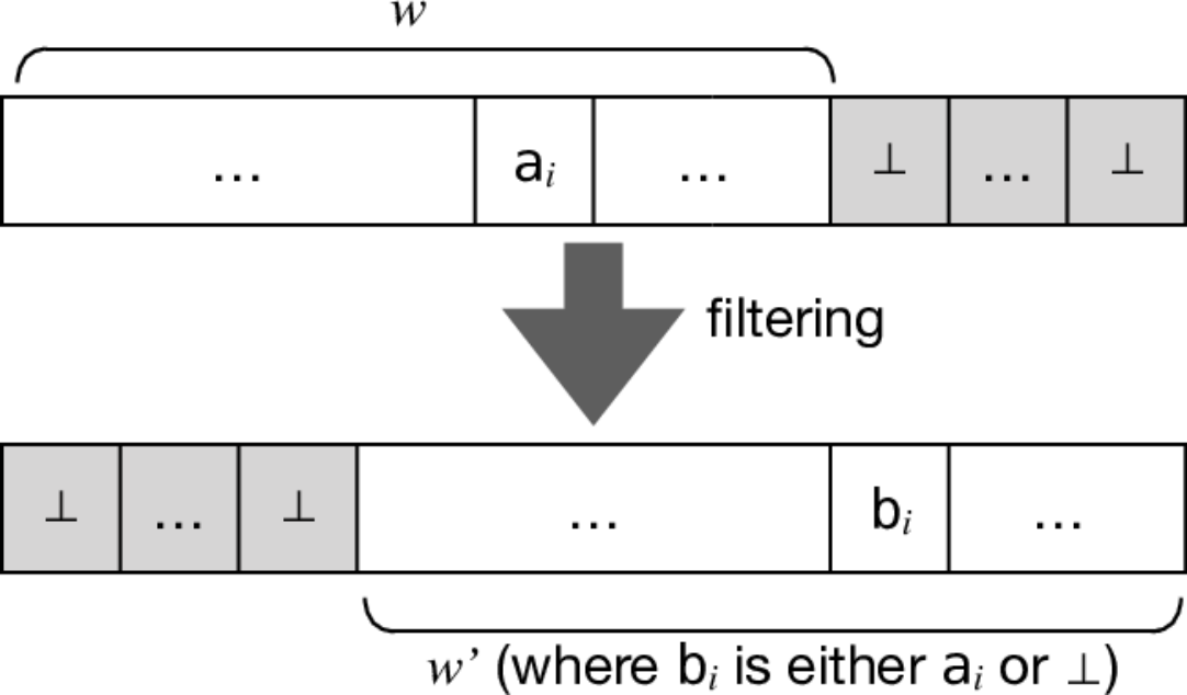
Fig. 4: Padding in filtering

Explanations are in order, especially about the buffer size NN and the padding by ⊥N\bot^{N} of the input and output words. The padding means filtering is done in the way depicted in Fig. 4, with a delay of NN steps. This is because of how our Moore machine works (Fig. 7): it scans the input word from left to right; the machine stores NN characters in the FIFO buffer in it (encoded in its state space QQ); and the characters are output once they are dequeued from the FIFO buffer. Hence there is a delay of NN steps. Initially, the buffer is filled with ⊥\bot (Fig. 7, Step 0); this accounts for the prefix ⊥N\bot^{N} of the output word ⊥Nw′\bot^{N}w^{\prime}. The padding ⊥N\bot^{N} at the end of the input word w⊥Nw\bot^{N} is needed to dequeue the content of the buffer (from Step n+1n+1 to n+Nn+N). In the course of the scanning in Fig. 7, some characters in w=a1​…​aNw=a_{1}\dotsc a_{N} get masked, although such masking is not explicit in the figure.

Refer to caption
Fig. 5: Filtering by a Moore machine. Sometimes a character aia_{i} is decided to be unnecessary and gets masked by ⊥\bot (i.e. bi=⊥b_{i}=\bot), although such masking is not explicit in the figure.
s0s_{0}starts1s_{1}s2s_{2}𝚊\tt a𝚋\tt b𝚊\tt a
(s0,0)(s_{0},0)startq0′q^{\prime}_{0}(s0,0),(s2,2)(s_{0},0),(s_{2},2)q3′q^{\prime}_{3}(s0,0),(s1,1)(s_{0},0),(s_{1},1)q1′q^{\prime}_{1}
(s0,0),(s1,1),(s_{0},0),(s_{1},1),
(s1,2)(s_{1},2)
q2′q^{\prime}_{2}
(s0,0),(s2,1),(s_{0},0),(s_{2},1),
(s2,2)(s_{2},2)
q4′q^{\prime}_{4}𝚋\tt b𝚊\tt a𝚊\tt a𝚋\tt b𝚊\tt a𝚊\tt a𝚋\tt b𝚋\tt b𝚊\tt a𝚋\tt b
Fig. 6: Left: a pattern NFA 𝒜0\mathcal{A}_{0} for 𝚊𝚊∗​𝚋\mathtt{aa}^{*}\mathtt{b}.   Right: the filter Moore machine ℳ𝒜0,2\mathcal{M}_{\mathcal{A}_{0},2}, its non-buffer part
(q0′,⊥⊥𝗆𝖺𝗌𝗄𝗆𝖺𝗌𝗄)→⊥𝚊(q1′,⊥𝚊𝗆𝖺𝗌𝗄𝗆𝖺𝗌𝗄)→⊥𝚋(q3′,𝚊𝚋𝗉𝖺𝗌𝗌𝗉𝖺𝗌𝗌)→𝚊𝚋(q0′,𝚋𝚋𝗉𝖺𝗌𝗌𝗆𝖺𝗌𝗄)→𝚋𝚋(q0′,𝚋𝚋𝗆𝖺𝗌𝗄𝗆𝖺𝗌𝗄)→⊥𝚊(q1′,𝚋𝚊𝗆𝖺𝗌𝗄𝗆𝖺𝗌𝗄)→⊥𝚊(q2′,𝚊𝚊𝗉𝖺𝗌𝗌𝗉𝖺𝗌𝗌)→𝚊𝚋(q4′,𝚊𝚋𝗉𝖺𝗌𝗌𝗉𝖺𝗌𝗌)→𝚊⊥({(s0,0)},𝚋⊥𝗉𝖺𝗌𝗌𝗆𝖺𝗌𝗄)→𝚋⊥({(s0,0)},⊥⊥𝗆𝖺𝗌𝗄𝗆𝖺𝗌𝗄)\begin{array}[]{l}\Bigl(q^{\prime}_{0},\,\begin{array}[]{|c|c|}\hline\cr\bot&\bot\\ \hline\cr\mathsf{mask}&\mathsf{mask}\\ \hline\cr\end{array}\,\Bigr)\xrightarrow[\bot]{\tt a}\Bigl(q^{\prime}_{1},\,\begin{array}[]{|c|c|}\hline\cr\bot&\tt a\\ \hline\cr\mathsf{mask}&\mathsf{mask}\\ \hline\cr\end{array}\,\Bigr)\\ \xrightarrow[\bot]{\tt b}\Bigl(q^{\prime}_{3},\,\begin{array}[]{|c|c|}\hline\cr\tt a&\tt b\\ \hline\cr\mathsf{pass}&\mathsf{pass}\\ \hline\cr\end{array}\,\Bigr)\xrightarrow[\tt a]{\tt b}\Bigl(q^{\prime}_{0},\,\begin{array}[]{|c|c|}\hline\cr\tt b&\tt b\\ \hline\cr\mathsf{pass}&\mathsf{mask}\\ \hline\cr\end{array}\,\Bigr)\\ \xrightarrow[\tt b]{\tt b}\Bigl(q^{\prime}_{0},\,\begin{array}[]{|c|c|}\hline\cr\tt b&\tt b\\ \hline\cr\mathsf{mask}&\mathsf{mask}\\ \hline\cr\end{array}\,\Bigr)\xrightarrow[\bot]{\tt a}\Bigl(q^{\prime}_{1},\,\begin{array}[]{|c|c|}\hline\cr\tt b&\tt a\\ \hline\cr\mathsf{mask}&\mathsf{mask}\\ \hline\cr\end{array}\,\Bigr)\\ \xrightarrow[\bot]{\tt a}\Bigl(q^{\prime}_{2},\,\begin{array}[]{|c|c|}\hline\cr\tt a&\tt a\\ \hline\cr\mathsf{pass}&\mathsf{pass}\\ \hline\cr\end{array}\,\Bigr)\xrightarrow[\tt a]{\tt b}\Bigl(q^{\prime}_{4},\,\begin{array}[]{|c|c|}\hline\cr\tt a&\tt b\\ \hline\cr\mathsf{pass}&\mathsf{pass}\\ \hline\cr\end{array}\,\Bigr)\\ \xrightarrow[\tt a]{\bot}\Bigl(\{(s_{0},0)\},\,\begin{array}[]{|c|c|}\hline\cr\tt b&\bot\\ \hline\cr\mathsf{pass}&\mathsf{mask}\\ \hline\cr\end{array}\,\Bigr)\xrightarrow[\tt b]{\bot}\Bigl(\{(s_{0},0)\},\,\begin{array}[]{|c|c|}\hline\cr\bot&\bot\\ \hline\cr\mathsf{mask}&\mathsf{mask}\\ \hline\cr\end{array}\,\Bigr)\end{array}
Fig. 7: The run of ℳ𝒜0,2\mathcal{M}_{\mathcal{A}_{0},2} over the word w=𝚊𝚋𝚋𝚋𝚊𝚊𝚋w=\mathtt{abbbaab}. The tables show the states of the buffer, enqueued from the right. In →𝑏𝑎\xrightarrow[b]{a}, aa is the input character and bb is the output character.

III-B Construction of Filter Moore Machine ℳ𝒜,N\mathcal{M}_{\mathcal{A},N}

Definition III.3 (the filter ℳ𝒜,N\mathcal{M}_{\mathcal{A},N} for (untimed) pattern matching).

Let Σ\Sigma be an alphabet, NN be a positive integer, and 𝒜=(Σ,S,s0,SF,E)\mathcal{A}=(\Sigma,S,s_{0},S_{F},E) be an NFA. We define a Moore machine

ℳ𝒜,N=(Σ⊥,Σ⊥,Q,q0,Δ,Λ)\mathcal{M}_{\mathcal{A},N}=(\Sigma_{\bot},\Sigma_{\bot},Q,q_{0},\Delta,\Lambda)

as follows. Its input and output alphabets are both Σ⊥\Sigma_{\bot}.

The state space is Q=𝒫⁡(S×(ℤ/N​ℤ))×((Σ⊥)N×{𝗉𝖺𝗌𝗌,𝗆𝖺𝗌𝗄}N)Q=\mathcal{P}\bigl(\,S\times(\mathbb{Z}/N\mathbb{Z})\,\bigr)\times\bigl((\Sigma_{\bot})^{N}\times\{\mathsf{pass},\mathsf{mask}\}^{N}\bigr). Here ℤ/N​ℤ\mathbb{Z}/N\mathbb{Z} is the NN-element set with addition modulo NN (§II).

The initial state is q0=({(s0,0)},(⊥,…,⊥),(𝗆𝖺𝗌𝗄,…,𝗆𝖺𝗌𝗄))q_{0}=\bigl(\,\bigl\{(s_{0},0)\bigr\},\,(\bot,\dotsc,\bot),\,(\mathsf{mask},\dotsc,\mathsf{mask})\,\bigr).

The transition Δ:Q×Σ⊥→Q\Delta\colon Q\times\Sigma_{\bot}\to Q is as follows. For each a∈Σ⊥a\in\Sigma_{\bot},

Δ⁡((𝒮,(a1,a2,…,aN),(l1,l2,…,lN)),a)=(𝒮′,(a2,…,aN,a),l¯), where\displaystyle\begin{array}[]{l}\Delta\Bigl(\,\bigl(\mathcal{S},(a_{1},a_{2},\dots,a_{N}),(l_{1},l_{2},\dots,l_{N})\bigr),\,a\,\Bigr)\\ \qquad\qquad\qquad=\bigl(\,\mathcal{S}^{\prime},\,(a_{2},\dots,a_{N},a),\,\overline{l}\,\bigr)\kern 5.0pt,\quad\text{ where}\end{array}
𝒮′={(s′,(nmodN)+1)∣(s,n)∈𝒮,(s,a,s′)∈E}∪{(s0,0)}, and\displaystyle\begin{aligned} \mathcal{S}^{\prime}=\bigl\{\,(s^{\prime},(n\bmod N)+1)\mid(s,n)&\in\mathcal{S},(s,a,s^{\prime})\in E\,\bigr\}\\ &\cup\{(s_{0},0)\}\kern 5.0pt,\text{ and}\end{aligned} (5)
l¯={(𝗉𝖺𝗌𝗌,…,𝗉𝖺𝗌𝗌)if ∃s.(s,N)∈𝒮′,(l2,l3,…,lN−ψ⁡(𝒮′)+1,𝗉𝖺𝗌𝗌,…,𝗉𝖺𝗌𝗌⏞ψ⁡(𝒮′))else if ∃n,s∈SF.  (s,n)∈𝒮′,(l2,l3,…,lN,𝗆𝖺𝗌𝗄)otherwise.\displaystyle\overline{l}=\footnotesize\begin{cases}(\mathsf{pass},\dotsc,\mathsf{pass})&\text{if $\exists s.\,(s,N)\in\mathcal{S}^{\prime}$,}\\ (l_{2},l_{3},\dots,l_{N-\psi(\mathcal{S}^{\prime})+1},\overbrace{\mathsf{pass},\dotsc,\mathsf{pass}}^{\psi(\mathcal{S}^{\prime})})&\text{else if $\exists n,s\in S_{F}.\,$ }\\ &\text{ $(s,n)\in\mathcal{S}^{\prime}$,}\\ (l_{2},l_{3},\dots,l_{N},\mathsf{mask})&\text{otherwise.}\end{cases} (6)

Here ψ⁡(𝒮′)∈ℤ>0\psi(\mathcal{S}^{\prime})\in{\mathbb{Z}}_{>0} is ψ(𝒮′)=max{n∣∃s∈SF.(s,n)∈𝒮′}\psi(\mathcal{S}^{\prime})=\max\{n\mid\exists s\in S_{F}.\,(s,n)\in\mathcal{S}^{\prime}\}.

Finally, the output function Λ:Q→Σ⊥\Lambda\colon Q\to\Sigma_{\bot} is defined as follows.

Λ⁡(𝒮,(a1,a2,…,aN),(l1,l2,…,lN))={a1if ​l1=𝗉𝖺𝗌𝗌⊥if ​l1=𝗆𝖺𝗌𝗄\Lambda\bigl(\,\mathcal{S},\,(a_{1},a_{2},\dotsc,a_{N}),\,(l_{1},l_{2},\dotsc,l_{N})\,\bigr)=\begin{cases}a_{1}&\text{if }l_{1}=\mathsf{pass}\\ \bot&\text{if }l_{1}=\mathsf{mask}\end{cases} (7)

We describe intuitions. The construction of ℳ𝒜,N\mathcal{M}_{\mathcal{A},N} combines three building blocks: determinization, counters and a buffer of size NN.

(Determinization) The pattern 𝒜\mathcal{A} is an NFA, but we want a deterministic Moore machine. This determinization accounts for the powerset construction 𝒫\mathcal{P} in the component 𝒫⁡(S×(ℤ/N​ℤ))\mathcal{P}\bigl(\,S\times(\mathbb{Z}/N\mathbb{Z})\,\bigr) of the state space QQ. For example, an element {(s1,n1),…,(sk,nk)}\{\,(s_{1},n_{1}),\dotsc,(s_{k},n_{k})\,\} of this component means “the states s1,…,sks_{1},\dotsc,s_{k} are active in the NFA 𝒜\mathcal{A}.” Observe that, in (5), the part regarding states (s,s′,…s,s^{\prime},\dotsc) follows the usual determinization. An exception is the addition of (s0,0)(s_{0},0) in (5): it is because a matching can start at any position of the input word.

(Counters) Moreover, each active state that traverses 𝒜\mathcal{A} keeps a counter for how many steps it has traveled since the initial state. This is the component ℤ/N​ℤ\mathbb{Z}/N\mathbb{Z} in the state space QQ. The maximum value of those counters is the same as the buffer size NN. Once this maximum is reached, a counter starts over from 11. See (5), where counters for active states are incremented modulo NN.

(Buffer) A FIFO buffer of size NN accounts for the second component (Σ⊥)N×{𝗉𝖺𝗌𝗌,𝗆𝖺𝗌𝗄}N(\Sigma_{\bot})^{N}\times\{\mathsf{pass},\mathsf{mask}\}^{N} of the state space QQ. Each of the NN cells stores a character from Σ⊥\Sigma_{\bot} and a label (𝗉𝖺𝗌𝗌\mathsf{pass} or 𝗆𝖺𝗌𝗄\mathsf{mask}). See (III.3) and  (6), where the basic behavior of the buffer is to dequeue the leftmost element and to enqueue the read character on the right.

It is the labels in the buffer (𝗉𝖺𝗌𝗌\mathsf{pass} or 𝗆𝖺𝗌𝗄\mathsf{mask}) that determine whether to mask a character or not. The default label is 𝗆𝖺𝗌𝗄\mathsf{mask} (the third case in (6)), and if it remains unchanged for NN steps then the corresponding character gets masked by ⊥\bot in the output (the second case in (7)). The label can change from 𝗆𝖺𝗌𝗄\mathsf{mask} to 𝗉𝖺𝗌𝗌\mathsf{pass} for two different reasons (the first two cases in (6)).

  • •

    The second case in (6) is when it is detected that some characters towards the end of the buffer form a match against the pattern 𝒜\mathcal{A}, leading to an accepting state s∈SFs\in S_{F} of 𝒜\mathcal{A}. Then we mark those characters by 𝗉𝖺𝗌𝗌\mathsf{pass}, indicating that they need to be passed to pattern matching (Fig. 3). The number ψ⁡(𝒮′)\psi(\mathcal{S}^{\prime}) of characters to be passed is calculated using the counter nn associated to the active state s∈SFs\in S_{F}.

  • •

    On the first case in (6), its condition ∃s.(s,N)∈𝒮′\exists s.\,(s,N)\in\mathcal{S}^{\prime} says that the counter for some active state ss has reached the maximum NN. In this case we are not sure whether this active state ss of 𝒜\mathcal{A} will eventually reach an accepting state or not. To be on the safe side, we pass all the NN characters to pattern matching without masking them. In the untimed setting, this is the only place where completeness of filtering is potentially lost.

In summary, in Def. III.3 we construct a Moore machine that works in the way depicted in Fig. 7. The Moore machine’s state space combines the following: determinization of the pattern NFA 𝒜\mathcal{A}; counters for the steps from the initial state; and a FIFO buffer that stores NN characters labeled by 𝗉𝖺𝗌𝗌\mathsf{pass} or 𝗆𝖺𝗌𝗄\mathsf{mask}.

Proposition III.4.

The Moore machine ℳ𝒜,N\mathcal{M}_{\mathcal{A},N} is a filter for 𝒜\mathcal{A} with buffer size NN, in the sense of Def. III.2. ∎

In our implementation, we realize a filter not as a plain Moore machine with a state space Q=𝒫⁡(S×(ℤ/N​ℤ))×((Σ⊥)N×{𝗉𝖺𝗌𝗌,𝗆𝖺𝗌𝗄}N)Q=\mathcal{P}(S\times(\mathbb{Z}/N\mathbb{Z}))\times((\Sigma_{\bot})^{N}\times\{\mathsf{pass},\mathsf{mask}\}^{N}) as described in Def. III.2. Instead, we separate the state space QQ into the “buffer part” (Σ⊥)N×{𝗉𝖺𝗌𝗌,𝗆𝖺𝗌𝗄}N(\Sigma_{\bot})^{N}\times\{\mathsf{pass},\mathsf{mask}\}^{N} and the “non-buffer part” 𝒫⁡(S×(ℤ/N​ℤ))\mathcal{P}(S\times({\mathbb{Z}}/N{\mathbb{Z}})), and we generate the former buffer part on-the-fly. More specifically, the non-buffer part is constructed as a DFA all at once in the beginning, and this DFA dictates how to operate on the buffer part that is realized as an array of size NN. See Example III.6 later for illustration.

Proposition III.5.

Let 𝒜=(Σ,S,s0,SF,E)\mathcal{A}=(\Sigma,S,s_{0},S_{F},E) be an NFA. For the induced filter Moore machine ℳ𝒜,N\mathcal{M}_{\mathcal{A},N}, the size of the non-buffer part 𝒫⁡(S×(ℤ/N​ℤ))\mathcal{P}(S\times({\mathbb{Z}}/N{\mathbb{Z}})) of its state space is bounded by O⁡(2N⋅|S|)O(2^{N\cdot|S|}).

Therefore, the memory usage for the non-buffer part (including the transitions) is O⁡(2N⋅|S|⋅|Σ|)O(2^{N\cdot|S|}\cdot|\Sigma|). The memory usage for the buffer part is O⁡(N​log⁡|Σ|)O(N\log|\Sigma|); overall, the space complexity of running our filter Moore machine ℳ𝒜,N\mathcal{M}_{\mathcal{A},N} is O⁡(2N⋅|S|⋅|Σ|)O(2^{N\cdot|S|}\cdot|\Sigma|). ∎

The space complexity is exponential in NN, and this comes from the powerset construction for the non-buffer part 𝒫⁡(S×(ℤ/N​ℤ))\mathcal{P}(S\times({\mathbb{Z}}/N{\mathbb{Z}})). Experimentally, however, the memory consumption does not necessarily grow exponentially in NN. This is because not all states in 𝒫⁡(S×(ℤ/N​ℤ))\mathcal{P}(S\times({\mathbb{Z}}/N{\mathbb{Z}})) are reachable. See RQ2 in §V.

Example III.6.

Let us consider the pattern 𝚊𝚊∗​𝚋\mathtt{aa}^{*}\mathtt{b}. It is expressed by the NFA 𝒜0\mathcal{A}_{0} in Fig. 7. The filter Moore machine ℳ𝒜0,2\mathcal{M}_{\mathcal{A}_{0},2} from Def. III.3 is depicted in Fig. 7, where buffer states are omitted. Its run over the word w=𝚊𝚋𝚋𝚋𝚊𝚊𝚋w=\mathtt{abbbaab} is shown in Fig. 7; its output word is ⊥⊥𝚊𝚋⊥⊥𝚊𝚊𝚋\bot\bot\mathtt{ab\bot\bot aab}, which means that the filtering result is 𝚊𝚋⊥⊥𝚊𝚊𝚋\mathtt{ab\bot\bot aab}.

III-C Properties of the Moore Machine ℳ𝒜,N\mathcal{M}_{\mathcal{A},N}

Throughout the rest of this section, let 𝒜\mathcal{A} be a pattern NFA 𝒜=(Σ,S,S0,E,SF)\mathcal{A}=(\Sigma,S,S_{0},E,S_{F}), NN be a positive integer, and ℳ𝒜,N=(Σ⊥,Σ⊥,Q,q0,Δ,Λ)\mathcal{M}_{\mathcal{A},N}=(\Sigma_{\bot},\Sigma_{\bot},Q,q_{0},\Delta,\Lambda) be the filter Moore machine in Def. III.3. Let w=a1​a2​…​anw=a_{1}a_{2}\dotsc a_{n} be a word over Σ\Sigma, and ⊥Nw′\bot^{N}w^{\prime} be the output word of ℳ𝒜,N\mathcal{M}_{\mathcal{A},N} over the input word w⊥Nw\bot^{N}. Let w′=b1​b2​…​bnw^{\prime}=b_{1}b_{2}\dots b_{n}, where bi∈Σ⊥b_{i}\in\Sigma_{\bot}.

Theorem III.7 (soundness).

The Moore machine ℳ𝒜,N\mathcal{M}_{\mathcal{A},N} is sound, in the sense of Def. III.2. ∎

Completeness holds if, the length of matches is bounded and the buffer size NN is no shorter than the bound. This is essentially the setting of multiple string matching [10].

Theorem III.8 (completeness).

Assume we have max⁡{|w|∣w∈L⁡(𝒜)}≤N<∞\max\{|w|\mid w\in L(\mathcal{A})\}\leq N<\infty. Then we can construct an NFA 𝒜′\mathcal{A}^{\prime} with L⁡(𝒜)=L⁡(𝒜′)L(\mathcal{A})=L(\mathcal{A}^{\prime}), so that the filter Moore machine ℳ𝒜′,N\mathcal{M}_{\mathcal{A}^{\prime},N} is complete. The latter means: if the index kk satisfies ak=bka_{k}=b_{k}, then there is an interval [i,j][i,j] such that k∈[i,j]k\in[i,j] and w|[i,j]∈L⁡(𝒜)w|_{[i,j]}\in L(\mathcal{A}). ∎

The intuition for monotonicity is that, the bigger the buffer size N′N^{\prime} is, the filter ℳ𝒜,N′\mathcal{M}_{\mathcal{A},N^{\prime}} masks more characters while its state space grows. A precise statement is more intricate, requiring the bigger buffer size N′′N^{\prime\prime} to be a multiple of the smaller one.

Theorem III.9 (monotonicity).

For any positive integer N′N^{\prime}, let ℳ𝒜,N′\mathcal{M}_{\mathcal{A},N^{\prime}} be the filter Moore machine of Def. III.3, and ⊥N′w′(N′)\bot^{N^{\prime}}w^{\prime(N^{\prime})} be the output word of ℳ𝒜,N′\mathcal{M}_{\mathcal{A},N^{\prime}} over the input word w⊥N′w\bot^{N^{\prime}}. Let w′(N′)=b1(N′)​b2(N′)​…​bn(N′)w^{\prime(N^{\prime})}=b^{(N^{\prime})}_{1}b^{(N^{\prime})}_{2}\dotsc b^{(N^{\prime})}_{n} where bi(N′)∈Σ⊥b^{(N^{\prime})}_{i}\in\Sigma_{\bot}. For any positive integers n,N′n,N^{\prime} and any index kk of ww, b(N′)k=⊥b^{(N^{\prime})}_{k}=\bot implies b(n​N′)k=⊥b^{(nN^{\prime})}_{k}=\bot. ∎

As mentioned in Prop. III.5, the state space of our filter Moore machine is exponentially bigger than that of 𝒜\mathcal{A}. This is because of the powerset construction required by its deterministic branching. By sacrificing the execution time, one can determinize the NFA on the fly, which usually needs less memory space. See Appendix B of [21].

IV Moore-Machine Filtering for Pattern Matching II: Timed

We present our main contribution, that is, the construction of filter Moore machines for timed pattern matching. While the basic ideas stay the same as in the untimed setting (§III), determinization poses a technical challenge, since timed automata (TA) cannot determinized in general [22]. Here we rely on one-clock determinization [11, §5.3]. The construction overapproximates reachability, hence we maintain soundness of filtering. Moreover, the local nature of the resulting TA—it has only one clock variable that is reset at every transition—allows us to devise a filter that is an untimed, finite-state Moore machine.

IV-A Problem Formulation

Definition IV.1 (timed words).

Let Σ\Sigma be an alphabet. A timed word over Σ\Sigma is a sequence ww of pairs (ai,τi)∈Σ×ℝ>0(a_{i},\tau_{i})\in\Sigma\times{\mathbb{R}}_{>0} satisfying τi<τi+1\tau_{i}<\tau_{i+1} for any i∈[1,|w|−1]i\in[1,|w|-1]. Let w=(a¯,τ¯)w=(\overline{a},\overline{\tau}) be a timed word. The set of timed words over Σ\Sigma is denoted by 𝒯⁡(Σ)\mathcal{T}(\Sigma).

We denote the subsequence (ai,τi),(ai+1,τi+1),⋯,(aj,τj)(a_{i},\tau_{i}),(a_{i+1},\tau_{i+1}),\cdots,(a_{j},\tau_{j}) by w⁡(i,j)w(i,j). For t∈ℝ≥0t\in{\mathbb{R}}_{\geq 0}, the tt-shift of ww is (a¯,τ¯)+t=(a¯,τ¯+t)(\overline{a},\overline{\tau})+t=(\overline{a},\overline{\tau}+t) where τ¯+t=(τ1+t,τ2+t,⋯,τ|τ|+t)\overline{\tau}+t=(\tau_{1}+t,\tau_{2}+t,\cdots,\tau_{|\tau|}+t). For timed words w=(a¯,τ¯)w=(\overline{a},\overline{\tau}) and w′=(a′¯,τ′¯)w^{\prime}=(\overline{a^{\prime}},\overline{\tau^{\prime}}), their absorbing concatenation is w∘w′=(a¯∘a′¯,τ¯∘τ′¯)w\circ w^{\prime}=(\overline{a}\circ\overline{a^{\prime}},\overline{\tau}\circ\overline{\tau^{\prime}}) where a¯∘a′¯\overline{a}\circ\overline{a^{\prime}} and τ¯∘τ′¯\overline{\tau}\circ\overline{\tau^{\prime}} are usual concatenations, and their non-absorbing concatenation is w⋅w′=w∘(w′+τ|w|)w\cdot w^{\prime}=w\circ(w^{\prime}+\tau_{|w|}). We note that the absorbing concatenation w∘w′w\circ w^{\prime} is defined only when τ|w|<τ1′\tau_{|w|}<\tau^{\prime}_{1}.

For a timed word w=(a¯,τ¯)w=(\overline{a},\overline{\tau}) on Σ\Sigma and t,t′∈ℝ>0t,t^{\prime}\in{\mathbb{R}}_{>0} satisfying t<t′t<t^{\prime}, a timed word segment w|(t,t′)w|_{(t,t^{\prime})} is defined by the timed word (w⁡(i,j)−t)∘($,t′−t)(w(i,j)-t)\circ(\$,t^{\prime}-t) on the augmented alphabet Σ∐{$}\Sigma\amalg\{\$\}, where i,ji,j are chosen so that τi−1≤t<τi\tau_{i-1}\leq t<\tau_{i} and τj<t′≤τj+1\tau_{j}<t^{\prime}\leq\tau_{j+1}. Here the timed word w⁡(i,j)−tw(i,j)-t is the (−t)(-t)-shift of w⁡(i,j)w(i,j); and the fresh symbol ${\$} is called the terminal character.

Definition IV.2 (timed automaton).

Let CC be a finite set of clock variables, and Φ⁡(C)\Phi(C) denote the set of conjunctions of inequalities x⋈cx\bowtie c where x∈Cx\in C, c∈ℤ≥0c\in{\mathbb{Z}}_{\geq 0}, and ⋈∈{>,≥,<,≤}{\bowtie}\in\{>,\geq,<,\leq\}. A timed automaton 𝒜=(Σ,S,s0,SF,C,E)\mathcal{A}=(\Sigma,S,s_{0},S_{F},C,E) is a tuple where Σ\Sigma is an alphabet, SS is a finite set of states, s0∈Ss_{0}\in S is an initial state, SF⊆SS_{F}\subseteq S is a set of accepting states, and E⊆S×S×Σ×𝒫⁡(C)×Φ⁡(C)E\subseteq S\times S\times\Sigma\times\mathcal{P}(C)\times\Phi(C) is a set of transitions. The components of a transition (s,s′,a,λ,δ)∈E(s,s^{\prime},a,\lambda,\delta)\in E represent: the source, target, action, reset variables and guard of the transition, respectively.

We define a clock valuation ν\nu as a function ν:C→ℝ≥0\nu:C\to{\mathbb{R}}_{\geq 0}. We define the tt-shift ν+t\nu+t of a clock valuation ν\nu, where t∈ℝ≥0t\in{\mathbb{R}}_{\geq 0}, by (ν+t)​(x)=ν​(x)+t(\nu+t)(x)=\nu(x)+t for any x∈Cx\in C. For a timed automaton 𝒜=(Σ,S,s0,SF,C,E)\mathcal{A}=(\Sigma,S,s_{0},S_{F},C,E) and a timed word w=(a¯,τ¯)w=(\overline{a},\overline{\tau}), a run of 𝒜\mathcal{A} over ww is a sequence rr of pairs (si,νi)∈S×(ℝ≥0)C(s_{i},\nu_{i})\in S\times({\mathbb{R}}_{\geq 0})^{C} satisfying the following: (initiation) s0s_{0} is the initial state and ν0​(x)=0\nu_{0}(x)=0 for any x∈Cx\in C; and (consecution) for any i∈[1,|w|]i\in[1,|w|], there exists a transition (si−1,si,ai,λ,δ)∈E(s_{i-1},s_{i},a_{i},\lambda,\delta)\in E such that νi−1+τi−τi−1⊧δ\nu_{i-1}+\tau_{i}-\tau_{i-1}\models\delta and νi​(x)=0\nu_{i}(x)=0 (for x∈λx\in\lambda) and νi​(x)=νi−1​(x)+τi−τi−1\nu_{i}(x)=\nu_{i-1}(x)+\tau_{i}-\tau_{i-1} (for x∉λx\not\in\lambda). A run only satisfying the consecution condition is a path. A run r=(s¯,ν¯)r=(\overline{s},\overline{\nu}) is accepting if the last element s|s|−1s_{|s|-1} of ss belongs to SFS_{F}. The language L⁡(𝒜)L(\mathcal{A}) is defined to be the set {w∣ there is an accepting run of 𝒜 over w}\{w\mid\text{ there is an accepting run of $\mathcal{A}$ over $w$}\} of timed words.

Here is our target problem. Its algorithms have been actively studied [3, 4, 6]; filtering Moore machines as preprocessors for those algorithms is this paper’s contribution.

Definition IV.3 (timed pattern matching).

Let 𝒜\mathcal{A} be a timed automaton, and ww be a timed word, over a common alphabet Σ\Sigma. The timed pattern matching problem requires all the intervals (t,t′)(t,t^{\prime}) for which the segment w|(t,t′)w|_{(t,t^{\prime})} is accepted by 𝒜\mathcal{A}. That is, it requires the match set Match⁡(w,𝒜)={(t,t′)∣w|(t,t′)∈L⁡(𝒜)}\mathrm{Match}(w,\mathcal{A})=\{(t,t^{\prime})\mid w|_{(t,t^{\prime})}\in L(\mathcal{A})\}.

IV-B One-Clock Determinization of TA

Among the three main building blocks for our untimed construction of filter (Def. III.3), counters and a buffer carry over smoothly to the current timed setting. For determinization we rely on the overapproximating notion in Def. IV.5; it is taken from [11, §5.3].

We start with some auxiliary notations.

Definition IV.4 (restriction ν|C\nu|_{C}, join ν⊔ν′\nu\sqcup\nu^{\prime}).

Let ν:C′→ℝ≥0\nu\colon C^{\prime}\to{\mathbb{R}}_{\geq 0} be a clock valuation. The restriction of ν\nu to C⊆C′C\subseteq C^{\prime} is denoted by ν|C:C→ℝ≥0\nu|_{C}\colon C\to{\mathbb{R}}_{\geq 0}. That is, (ν|C)​(x)=ν⁡(x)(\nu|_{C})(x)=\nu(x) for each x∈Cx\in C.

Let ν:C→ℝ≥0\nu\colon C\to{\mathbb{R}}_{\geq 0} and ν′:C′→ℝ≥0\nu^{\prime}\colon C^{\prime}\to{\mathbb{R}}_{\geq 0} be clock variations. We define their join ν⊔ν′:C∐C′→ℝ≥0\nu\sqcup\nu^{\prime}\colon C\amalg C^{\prime}\to{\mathbb{R}}_{\geq 0} to be the following clock valuation over the disjoint union C∐C′C\amalg C^{\prime}.

(ν⊔ν′)​(x)={ν⁡(x)if x∈Cν′​(x)if x∈C′.\displaystyle(\nu\sqcup\nu^{\prime})(x)=\begin{cases}\nu(x)&\text{if $x\in C$}\\ \nu^{\prime}(x)&\text{if $x\in C^{\prime}$.}\end{cases}

The function that maps xix_{i} to rir_{i} (for each i∈{1,…,n}i\in\{1,\dotsc,n\}) is denoted by [x1↦r1,…,xn↦rn][x_{1}\mapsto r_{1},\dotsc,x_{n}\mapsto r_{n}].

Definition IV.5 (one-clock determinization).

Let 𝒜=(Σ,S,s0,SF,C,E)\mathcal{A}=(\Sigma,S,s_{0},S_{F},C,E) be a timed automaton (TA), and yy be a fresh clock variable (i.e. y∉Cy\not\in C). A TA 𝒜′=(Σ,S′,s0′,SF′,{y},E′)\mathcal{A}^{\prime}=(\Sigma,S^{\prime},s^{\prime}_{0},S^{\prime}_{F},\{y\},E^{\prime}) is a one-clock determinization of 𝒜\mathcal{A} if the following conditions hold.

  1. 1.

    Each element 𝒮∈S′\mathcal{S}\in S^{\prime} of the (new, finite) state space S′S^{\prime} is a finite set 𝒮={(s1,Z1),…,(sm,Zm)}\mathcal{S}=\{(s_{1},Z_{1}),\dotsc,(s_{m},Z_{m})\} of pairs (si,Zi)(s_{i},Z_{i}), where si∈Ss_{i}\in S is a state of 𝒜\mathcal{A}, and ZiZ_{i} is a subset of (ℝ≥0)C∐{y}({\mathbb{R}}_{\geq 0})^{C\amalg\{y\}} given by a special polytope called a zone (see e.g. [23]).

  2. 2.

    For each transition (𝒮,a,δ,λ,𝒮′)∈E′(\mathcal{S},a,\delta,\lambda,\mathcal{S}^{\prime})\in E^{\prime} of 𝒜′\mathcal{A}^{\prime}, the guard δ\delta is a finite union of intervals of yy. Moreover it respects enabledness of transitions EE in 𝒜\mathcal{A}. Precisely, for any u,u′∈ℝ≥0u,u^{\prime}\in{\mathbb{R}}_{\geq 0} that satisfy δ\delta, we have Ea​(𝒮,u)=Ea​(𝒮,u′)E_{a}(\mathcal{S},u)=E_{a}(\mathcal{S},u^{\prime}), where the set Ea​(𝒮,u)⊆EE_{a}(\mathcal{S},u)\subseteq E is defined by

    Ea(𝒮,u)={(s,a,δ′,λ′,s′)∈E|∃(s,Z)∈𝒮.∃ν∈Z.ν(y)=u and ν satisfies δ′}.E_{a}(\mathcal{S},u)=\bigl\{\,(s,a,\delta^{\prime},\lambda^{\prime},s^{\prime})\in E\;\big|\;\\ \exists(s,Z)\in\mathcal{S}.\,\exists\nu\in Z.\,\nu(y)=u\text{ and $\nu$ satisfies $\delta^{\prime}$}\,\bigr\}\kern 5.0pt.
  3. 3.

    Each transition of 𝒜′\mathcal{A}^{\prime} resets the unique clock variable yy. That is, for each transition (𝒮,a,δ,λ,𝒮′)∈E′(\mathcal{S},a,\delta,\lambda,\mathcal{S}^{\prime})\in E^{\prime}, we have λ={y}\lambda=\{y\}.

  4. 4.

    Each transition (𝒮,a,δ,λ,𝒮′)∈E′(\mathcal{S},a,\delta,\lambda,\mathcal{S}^{\prime})\in E^{\prime} of 𝒜′\mathcal{A}^{\prime} simulates transitions of 𝒜\mathcal{A}. More precisely, let (s,Z)∈𝒮(s,Z)\in\mathcal{S} and (ν:C∐{y}→ℝ≥0)∈Z(\nu\colon C\amalg\{y\}\to{\mathbb{R}}_{\geq 0})\in Z. Assume that (s,ν|C)→a,τ(s′,ν′)(s,\nu|_{C})\xrightarrow{a,\tau}(s^{\prime},\nu^{\prime}) is a (length-1) path of 𝒜\mathcal{A}, for some s′∈Ss^{\prime}\in S and ν′:C→ℝ≥0\nu^{\prime}\colon C\to{\mathbb{R}}_{\geq 0} (here τ\tau is the dwell time). Then we require that there exist a zone Z′⊆(ℝ≥0)C∐{y}Z^{\prime}\subseteq({\mathbb{R}}_{\geq 0})^{C\amalg\{y\}} such that 1) (s′,Z′)∈𝒮′(s^{\prime},Z^{\prime})\in\mathcal{S}^{\prime} and 2) the valuation ν′⊔[y↦τ]\nu^{\prime}\sqcup[y\mapsto\tau], over the clock set C∐{y}C\amalg\{y\}, belongs to Z′Z^{\prime}.

  5. 5.

    𝒜′\mathcal{A}^{\prime} is deterministic: for each state 𝒮∈S′\mathcal{S}\in S^{\prime}, each clock valuation ν∈(ℝ≥0){y}\nu\in({\mathbb{R}}_{\geq 0})^{\{y\}}, a∈Σa\in\Sigma and τ∈ℝ≥0\tau\in{\mathbb{R}}_{\geq 0} for the dwell time, a length-1 path from (𝒮,ν)(\mathcal{S},\nu) labeled with a,τa,\tau is unique. That is, if (𝒮,ν)→a,τ(𝒮′,ν′)(\mathcal{S},\nu)\xrightarrow{a,\tau}(\mathcal{S}^{\prime},\nu^{\prime}) and (𝒮,ν)→a,τ(𝒮′′,ν′′)(\mathcal{S},\nu)\xrightarrow{a,\tau}(\mathcal{S}^{\prime\prime},\nu^{\prime\prime}) are both paths in 𝒜′\mathcal{A}^{\prime}, then 𝒮′=𝒮′′\mathcal{S}^{\prime}=\mathcal{S}^{\prime\prime} and ν′=ν′′\nu^{\prime}=\nu^{\prime\prime}. (Note that Cond. 3 forces ν′=ν′′=[y↦0]\nu^{\prime}=\nu^{\prime\prime}=[y\mapsto 0].)

  6. 6.

    The initial state s0′s^{\prime}_{0} of 𝒜′\mathcal{A}^{\prime} is given by s0′={(s0,{𝟎})}s^{\prime}_{0}=\{(s_{0},\{\mathbf{0}\})\}. Here 𝟎\mathbf{0} is the valuation that maps every clock variable to 00.

  7. 7.

    A state 𝒮\mathcal{S} belongs to SF′S^{\prime}_{F} if and only if there exists (s,Z)∈𝒮(s,Z)\in\mathcal{S} such that s∈SFs\in S_{F}.

Proposition IV.6.

Let 𝒜=(Σ,S,s0,SF,C,E)\mathcal{A}=(\Sigma,S,s_{0},S_{F},C,E) be a TA, and 𝒜′=(Σ,S′,s0′,SF′,{y},E′)\mathcal{A}^{\prime}=(\Sigma,S^{\prime},s^{\prime}_{0},S^{\prime}_{F},\{y\},E^{\prime}) be a one-clock determinization of 𝒜\mathcal{A}. Then 𝒜′\mathcal{A}^{\prime} satisfies the following properties.

  • •

    (Simulation) Let w∈𝒯⁡(Σ)w\in\mathcal{T}(\Sigma) be a timed word, and assume that there exists a run over ww to a state s∈Ss\in S in 𝒜\mathcal{A}. Then there exists 𝒮∈S′\mathcal{S}\in S^{\prime} that satisfies the following: 1) (s,Z)∈𝒮(s,Z)\in\mathcal{S} for some zone ZZ, and 2) there exists a run over ww to 𝒮\mathcal{S} in 𝒜′\mathcal{A}^{\prime}.

  • •

    (Language inclusion) In particular, L⁡(𝒜)⊆L⁡(𝒜′)L(\mathcal{A})\subseteq L(\mathcal{A}^{\prime}). ∎

Note that Def. IV.5 gives a property and not a construction: there are multiple one-clock determinizations—of varying size and precision—of the same TA 𝒜\mathcal{A}. In our implementation we use a specific construction presented in [11, §5.3.4]. A sketch is in Appendix C of [21].

IV-C Construction of Our Filter ℳ𝒜,N\mathcal{M}_{\mathcal{A},N}

Definition IV.7 (the filter ℳ𝒜,N\mathcal{M}_{\mathcal{A},N} for timed pattern matching).

Let 𝒜=(Σ,S,s0,SF,C,E)\mathcal{A}=(\Sigma,S,s_{0},S_{F},C,E) be a TA, and N∈ℤ>0N\in{\mathbb{Z}}_{>0}. The construction of the filter Moore machine ℳ𝒜,N\mathcal{M}_{\mathcal{A},N} is by the following steps.

In the first step we augment the original TA 𝒜\mathcal{A} with counters. Specifically, let 𝒜N​-​ctr=(Σ⊥,S×[0,N],(s0,0),SFN​-​ctr,C,EN​-​ctr)\mathcal{A}^{N\text{-}\mathrm{ctr}}=(\Sigma_{\bot},S\times[0,N],(s_{0},0),S^{N\text{-}\mathrm{ctr}}_{F},C,E^{N\text{-}\mathrm{ctr}}) be defined as follows. SFN​-​ctr={(sf,n)∣sf∈SF,n∈[0,N]}S^{N\text{-}\mathrm{ctr}}_{F}=\{(s_{f},n)\mid s_{f}\in S_{F},n\in[0,N]\}, and

EN​-​ctr={((s0,0),a,𝐭𝐫𝐮𝐞,C,(s0,0))|a∈Σ⊥}∪{((s,n),a,δ,λ,(s′,n+1))|(s,a,δ,λ,s′)∈E,n∈[0,N−1]}∪{((s,N),a,δ,λ,(s′,1))|(s,a,δ,λ,s′)∈E}.\displaystyle\small\begin{array}[]{l}E^{N\text{-}\mathrm{ctr}}=\bigl\{\,\bigl((s_{0},0),a,\mathbf{true},C,(s_{0},0)\bigr)\;\big|\;a\in\Sigma_{\bot}\,\bigr\}\\ \hskip 9.24994pt\cup\bigl\{\,\bigl((s,n),a,\delta,\lambda,(s^{\prime},n+1)\bigr)\;\big|\;(s,a,\delta,\lambda,s^{\prime})\in E,n\in[0,N-1]\,\bigr\}\\ \hskip 9.24994pt\cup\bigl\{\,\bigl((s,N),a,\delta,\lambda,(s^{\prime},1)\bigr)\;\big|\;(s,a,\delta,\lambda,s^{\prime})\in E\,\bigr\}\kern 4.62497pt.\end{array}

In the second step we take a one-clock determinization (Def. IV.5) of 𝒜N​-​ctr\mathcal{A}^{N\text{-}\mathrm{ctr}}. Let 𝒜N​-​ctr​-​d=(Σ⊥,SN​-​ctr​-​d,s0N​-​ctr​-​d,SFN​-​ctr​-​d,{y},EN​-​ctr​-​d)\mathcal{A}^{N\text{-}\mathrm{ctr\text{-}d}}=(\Sigma_{\bot},S^{N\text{-}\mathrm{ctr\text{-}d}},s_{0}^{N\text{-}\mathrm{ctr\text{-}d}},S_{F}^{N\text{-}\mathrm{ctr\text{-}d}},\{y\},E^{N\text{-}\mathrm{ctr\text{-}d}}) be the outcome.

Finally in the third step we define the Moore machine ℳ𝒜,N\mathcal{M}_{\mathcal{A},N}:

ℳ𝒜,N=(Σ⊥×ℝ≥0,{𝗉𝖺𝗌𝗌,𝗆𝖺𝗌𝗄},SN​-​ctr​-​d×{𝗉𝖺𝗌𝗌,𝗆𝖺𝗌𝗄}N,OPEN(s0N​-​ctr​-​d,(𝗆𝖺𝗌𝗄,…,𝗆𝖺𝗌𝗄)),Δ,Λ),\displaystyle\begin{array}[]{r}\mathcal{M}_{\mathcal{A},N}\;=\;\Bigl(\,\Sigma_{\bot}\times{\mathbb{R}}_{\geq 0},\,\{\mathsf{pass},\mathsf{mask}\},\,S^{N\text{-}\mathrm{ctr\text{-}d}}\times\{\mathsf{pass},\mathsf{mask}\}^{N},\\ \bigl(s_{0}^{N\text{-}\mathrm{ctr\text{-}d}},(\mathsf{mask},\dotsc,\mathsf{mask})\bigr),\,\Delta,\,\Lambda\,\Bigr)\kern 5.0pt,\end{array}

where Δ\Delta and Λ\Lambda are defined as follows. Δ⁡((𝒮,l¯),(a,τ))=(𝒮′,l¯′)\Delta\bigl(\,(\mathcal{S},\overline{l}),\,(a,\tau)\,\bigr)=(\mathcal{S^{\prime}},\overline{l}^{\prime}), where 𝒮′\mathcal{S^{\prime}} is the unique successor of 𝒮\mathcal{S} in 𝒜N​-​ctr​-​d\mathcal{A}^{N\text{-}\mathrm{ctr\text{-}d}} under the character aa and the dwell time τ\tau (Def. IV.5), and l¯′\overline{l}^{\prime} is defined as follows.

l¯′={𝗉𝖺𝗌𝗌Nif ∃s,Z.((s,N),Z)∈𝒮l2,l3,…,lN−ψ⁡(𝒮′)+1,𝗉𝖺𝗌𝗌,…,𝗉𝖺𝗌𝗌⏞ψ⁡(𝒮′)else if ∃((s,n),Z)∈𝒮.s∈SF l2,l3,…,lN,𝗆𝖺𝗌𝗄otherwise\footnotesize\begin{array}[]{l}\overline{l}^{\prime}=\begin{cases}\mathsf{pass}^{N}&\text{if $\exists s,Z.\,\bigl((s,N),Z\bigr)\in\mathcal{S}$}\\ l_{2},l_{3},\dots,l_{N-\psi(\mathcal{S}^{\prime})+1},\overbrace{\mathsf{pass},\dotsc,\mathsf{pass}}^{\psi(\mathcal{S}^{\prime})}&\text{else if $\exists((s,n),Z)\in\mathcal{S}.\,s\in S_{F}$ }\\ l_{2},l_{3},\dots,l_{N},\mathsf{mask}&\text{otherwise}\end{cases}\end{array}

Here ψ(𝒮′)=max{n∣∃s,Z.((s,n),Z)∈𝒮 and s∈SF}\psi(\mathcal{S}^{\prime})=\max\{n\mid\exists s,Z.\,((s,n),Z)\in\mathcal{S}\text{ and }s\in S_{F}\}. We define Λ⁡((𝒮,(l1,l2,…,lN)))=l1\Lambda\bigl((\mathcal{S},(l_{1},l_{2},\dots,l_{N}))\bigr)=l_{1}.

[Uncaptioned image]

Note that the resulting Moore machine takes timed words as input. This makes its input alphabet infinite (namely Σ⊥×ℝ≥0\Sigma_{\bot}\times{\mathbb{R}}_{\geq 0}). This is not a big issue in implementation: we note that the state space is still finite. Moreover, the output alphabet of ℳ𝒜,N\mathcal{M}_{\mathcal{A},N} is a two-element set {𝗉𝖺𝗌𝗌,𝗆𝖺𝗌𝗄}\{\mathsf{pass},\mathsf{mask}\}, meaning that the filter Moore machine only outputs the masking information. A finite-state Moore machine is certainly not capable of buffering time-stamped characters, but the original timed word can be copied and suitable masking can be applied to it later. See the above figure.

Theorem IV.8 (soundness).

Let 𝒜\mathcal{A} be a pattern TA 𝒜=(Σ,S,s0,SF,C,E)\mathcal{A}=(\Sigma,S,s_{0},S_{F},C,E), NN be a positive integer, and ℳ𝒜,N\mathcal{M}_{\mathcal{A},N} be the filter Moore machine in Def. IV.7. Let w=(a1,τ1)​(a2,τ2)​…​(an,τn)w=(a_{1},\tau_{1})(a_{2},\tau_{2})\dotsc(a_{n},\tau_{n}) be a timed word over Σ\Sigma, and 𝗆𝖺𝗌𝗄N​w′\mathsf{mask}^{N}w^{\prime} be the output word of ℳ𝒜,N\mathcal{M}_{\mathcal{A},N} over the input word w​(⊥,τn)Nw(\bot,\tau_{n})^{N} (here the input and output words are padded by 𝗆𝖺𝗌𝗄N\mathsf{mask}^{N} and (⊥,τn)N(\bot,\tau_{n})^{N}, much like in Fig. 4). Let w′=b1​b2​…​bnw^{\prime}=b_{1}b_{2}\dots b_{n}, where bk∈{𝗉𝖺𝗌𝗌,𝗆𝖺𝗌𝗄}b_{k}\in\{\mathsf{pass},\mathsf{mask}\}.

For any pair (i,j)(i,j) of indices of ww satisfying w⁡(i,j)−τi−1∈L⁡(𝒜)w(i,j)-\tau_{i-1}\in L(\mathcal{A}) and for any index k∈[i,j]k\in[i,j] of ww, we have bk=𝗉𝖺𝗌𝗌b_{k}=\mathsf{pass}. ∎

V Implementation and Experiments

We implemented our filter construction for timed pattern matching. Our implementation suppresses successive ⊥\bot’s into two ⊥\bot’s, maintaining the timestamp of the first and the last ⊥\bot’s. We generate the buffer part of the state space QQ on-the-fly (namely {𝗉𝖺𝗌𝗌,𝗆𝖺𝗌𝗄}N\{\mathsf{pass},\mathsf{mask}\}^{N} of Def. IV.7); this is as we discussed before Prop. III.5. We conducted experiments to answer the following research questions.

  • RQ1:

    Does our filter Moore machine mask many events?

  • RQ2:

    Is our filter Moore machine online capable? That is, does it work in linear time and constant space, with respect to the length of the input timed word?

  • RQ3:

    Does our filter Moore machine accelerate the whole task of timed pattern matching?

  • RQ4:

    Is our filter precise? That is, do many of the non-masked events contribute to actual matches?

  • RQ5:

    Is our filter responsive? That is, does it not cause large delays?

We implemented our filter construction in C++ and compiled them by clang-900.0.39.2. The tool’s input consists of a pattern TA 𝒜\mathcal{A}, the buffer size NN and a timed word ww; it outputs a filtered word. The experiments are done on Mac OS 10.13.4, MacBook Pro Early 2013 with 2.6 GHz Intel Core i5 processor and 8 GB 1600MHz DDR3 RAM. The benchmark problems we used are in Fig. 8—10. All of them are from automotive scenarios.

For the measurement of the execution time and the memory usage, we used GNU time and took the average of 20 executions. In each experiment, we measured the whole workflow: in RQ2, the time and memory usage include that for constructing a filter; and in RQ3, the time and memory usage account for filter construction, filtering, process intercommunication, and pattern matching. In the experiments for RQ3, we used 𝙼𝙾𝙽𝙰𝙰{\mathtt{MONAA}} [20], a recent tool for timed pattern matching. See Appendix D of [21] for the detailed results.

s0s_{0}starts1s_{1}s2s_{2}s3s_{3}s4s_{4}s5s_{5}s6s_{6}
low,𝐭𝐫𝐮𝐞\textrm{low},\mathbf{true}
/x:=0/x:=0
high,\textrm{high},
0<x<10<x<1
high,\textrm{high},
0<x<10<x<1
high,\textrm{high},
0<x<10<x<1
high,\textrm{high},
0<x<10<x<1
high,\textrm{high},
1<x1<x
high,𝐭𝐫𝐮𝐞\textrm{high},\mathbf{true}
Fig. 8: Torque. The set WW (length 242,808–4,873,207) of input words is generated by the automotive engine model sldemo_enginewc.slx [24] with random input. The pattern specifies four or more consecutive occurrences of high in one second. For N=10N=10, the size of our filter Moore machine ℳ𝒜,10\mathcal{M}_{\mathcal{A},10}, measured by the number of the reachable states in the non-buffer part SN​-​ctr​-​dS^{N\text{-}\mathrm{ctr\text{-}d}} (cf. Def. IV.7 and Prop. III.5), is 1616.
startg1\text{g}_{1}g2\text{g}_{2}g1/x:=0\text{g}_{1}/x:=0g2,x<2\text{g}_{2},x<2
Fig. 9: Gear. The set WW (length 306–1,011,426) of input words is generated by the automatic transmission system model in [25]. The pattern, from ϕ5𝐴𝑇\phi^{\mathit{AT}}_{5} in [25], is for an event in which gear shift occurs too quickly (from the 1st to 2nd). For N=10N=10, the size of our filter Moore machine ℳ𝒜,10\mathcal{M}_{\mathcal{A},10}, measured in the same way of Fig. 8, is 33.
??startg1\text{g}_{1}??g2\text{g}_{2}g1\text{g}_{1}g3\text{g}_{3}g2\text{g}_{2}g4\text{g}_{4}g3\text{g}_{3}g4\text{g}_{4}✓g1,𝐭𝐫𝐮𝐞\text{g}_{1},\mathbf{true}g2,𝐭𝐫𝐮𝐞\text{g}_{2},\mathbf{true}g3,𝐭𝐫𝐮𝐞\text{g}_{3},\mathbf{true}g4,𝐭𝐫𝐮𝐞\text{g}_{4},\mathbf{true}ω≥2500,𝐭𝐫𝐮𝐞\omega\geq 2500,\mathbf{true}ω≥2500,𝐭𝐫𝐮𝐞\omega\geq 2500,\mathbf{true}ω≥2500,𝐭𝐫𝐮𝐞\omega\geq 2500,\mathbf{true}
ω≥2500,x<10\omega\geq 2500,x<10
/x:=0/x:=0
g1,𝐭𝐫𝐮𝐞\text{g}_{1},\mathbf{true}g2,𝐭𝐫𝐮𝐞\text{g}_{2},\mathbf{true}g3,𝐭𝐫𝐮𝐞\text{g}_{3},\mathbf{true}
g4,x<10\text{g}_{4},x<10
/x:=0/x:=0
ω≥2500,𝐭𝐫𝐮𝐞\omega\geq 2500,\mathbf{true}
ω​<2500,x>​1\omega<2500,x>1
ω≥2500,x>1\omega\geq 2500,x>1
g3,x>1\text{g}_{3},x>1
g4,x>1\text{g}_{4},x>1
ω<2500/x:=0\omega<2500/x:=0
ω≥2500/x:=0\omega\geq 2500/x:=0
g3/x:=0\text{g}_{3}/x:=0
g4/x:=0\text{g}_{4}/x:=0
ω<2500,𝐭𝐫𝐮𝐞\omega<2500,\mathbf{true}
ω≥2500,𝐭𝐫𝐮𝐞\omega\geq 2500,\mathbf{true}
g3,𝐭𝐫𝐮𝐞\text{g}_{3},\mathbf{true}
g4,𝐭𝐫𝐮𝐞\text{g}_{4},\mathbf{true}
ω​<2500,x>​1\omega<2500,x>1
ω≥2500,x>1\omega\geq 2500,x>1
g3,x>1\text{g}_{3},x>1
g4,x>1\text{g}_{4},x>1
Fig. 10: Accel. The set WW (length 708–1,739,535) of input words is generated by the same model as in Gear. The pattern is from ϕ8𝐴𝑇\phi^{\mathit{AT}}_{8} in [25]: the gear shifts from 1st to 4th and RPM gets high in its course, but the velocity is low (i.e. the event v≥100v\geq 100 is absent). For N=10N=10, the size of our filter Moore machine ℳ𝒜,10\mathcal{M}_{\mathcal{A},10}, measured in the same way of Fig. 8, is 7171.

Torque

Gear

Accel

Fig. 11: Length of the input and filtered timed words

Torque

Gear

Accel

Fig. 12: Execution time of our filter Moore machine (including time for construction of a filter)

Torque

Gear

Accel

Fig. 13: Memory usage of our filter Moore machine

Torque

Gear

Accel

Fig. 14: Execution time of the workflow in Fig. 3, with our filter and monitoring by 𝙼𝙾𝙽𝙰𝙰{\mathtt{MONAA}}

V-A RQ1: Filtering Rate

Fig. 11 shows the length of the filtered timed words by our filter Moore machine for each pattern timed automaton 𝒜\mathcal{A}, buffer size NN, and timed word w∈Ww\in W.

We observe that the filtered word gets shorter as NN is bigger. This concurs with our theoretical consideration in Theorem III.9 (although the result is for the untimed setting). It seems that peak performance is achieved with a relatively small NN, such as N=10N=10. With N=10N=10 the length of the filtered timed word is about 1/31/3, 1/21/2, and 1/1001/100 of that of the original timed word in Torque, Gear, and Accel respectively. For Accel our filter masks many characters, because the sizes of the alphabet and the pattern timed automaton are relatively large. This significant data reduction demonstrates the practical use of our filtering methodology in embedded usage scenarios (see Fig. 3).

V-B RQ2: Speed and Memory Usage

Fig. 12 and 13 show the execution time and memory usage of our filter Moore machine for each pattern timed automaton 𝒜\mathcal{A}, buffer size NN, and timed word w∈Ww\in W.

In Fig. 12, we observe that the execution time is linear to the length of the input word. In Fig. 13, the memory usage is more or less constant with respect to the length of the input word. These two results suggest that our filtering methodology is online capable.

The time for constructing a filter Moore machine is seen to be negligible: see the execution time for short input words in Fig. 12.

On the effect of varying the buffer size NN, for smaller NN the execution time was relatively large. This seems to be because fewer characters get masked, more characters are output, and this incurs I/O cost. On memory usage, despite the worst-case result in Prop. III.5 (exponential in NN), the growth for bigger NN was moderate. This is because not all states from the powerset construction are reachable.

V-C RQ3: Acceleration of Timed Pattern Matching

Fig. 14 shows the execution time of the workflow in Fig. 3, where the filter is given by our algorithm and pattern matching is done by a recent tool 𝙼𝙾𝙽𝙰𝙰{\mathtt{MONAA}} [20]. More specifically, we connect the standard output of the filter Moore machine to the standard input of 𝙼𝙾𝙽𝙰𝙰{\mathtt{MONAA}} by Unix pipeline. This way the filter and 𝙼𝙾𝙽𝙰𝙰{\mathtt{MONAA}} run parallelly on different cores.

We observe that, via filtering, the overall performance of timed pattern matching is accelerated when NN is large enough (say N=10N=10). For Torque and Gear, the speedup is 1.21.2 times; for Accel, it is roughly twice. This acceleration suggests that our filtering methodology is potentially beneficial independent of the architecture assumption in Fig. 3: when a log is enormous monitoring can take hours or days; by running a filter in parallel the time can be shortened.

V-D RQ4: Precision

For the three examples Torque, Gear, and Accel, and N=10N=10, the ratios of non-masked events contributing to actual matches were 0.34%, 99%, and 92% respectively. Therefore the precision differs greatly depending on patterns. It should also be noted that, even in the low-precision example (Torque), our filter successfully reduced the log size by approximately three times (Fig. 11).

Most of the imprecision in the current timed setting is attributed to the laxness of one-clock determinization (Def. IV.5). For example, the TA for Torque (Fig. 8) requires four consecutive occurrences of high within one second, using the same clock xx. The best overapproximation by one-clock determinization—in which all clock variables get reset after each transition—is to require an occurrence of high in each of four consecutive time segments of length ≤1\leq 1. This is a much looser requirement than the original, and explains the comparatively poorer precision in the example Torque.

V-E RQ5: Responsiveness

For the three examples Torque, Gear, Accel, and the buffer size N=10N=10, we calculated the average delay caused by our filter, which is (the execution time)/|w|×N\text{(the execution time)}/|w|\times N. The results were 2.2​μ​s2.2\,\mathrm{\mu s}, 3.1​μ​s3.1\,\mathrm{\mu s}, and 0.91​μ​s0.91\,\mathrm{\mu s} respectively. Although these delays highly depend on the computation power of the processor, the delays were tiny. We conclude our filter is responsive enough.

VI Related Work

Efficiency of pattern matching has been actively pursued in the fields of database [17, 18] and networking [26, 27, 28, 19, 12, 29]. In these fields, issues in hardware architecture—such as speed gap between L1/L2 caches and main memory—constitute situations similar to that of embedded monitors that we discussed in the above.

Many works in these application domains deal with (potentially multiple) strings as patterns. There the main source of inspiration is classic algorithms such as Boyer–Moore [30], Commentz-Walter [31], and Aho–Corasick [10]. Examples are e.g. in [32]. Many algorithms for patterns given by regular expressions or automata (instead of strings) also rely on those string-matching techniques. See e.g. [17].

In database and networking, pattern matching against regular expressions is mainly approached by application-specific heuristics that often take machine architecture into account. For example, in [26, 19] pattern regular expressions undergo application of some application-specific rewrite rules. The hierarchical structure of L1/L2 caches and main memory is exploited in [17, 18], while the features of content-addressable memory (CAM)—an alternative to RAM often used in network devices—are exploited in [12]. The work [29] extends the formalism of DFA by auxiliary variables for the purpose of moderating state space inflation when multiple patterns are combined.

Pre-filtering before actual pattern matching has been considered in the above lines of works [17, 32, 26]. The principal difference between those works and ours is that their filters produce match candidates, data that include explicit indices for potential matches. For this reason, the second step of the workflow (what we call pattern matching) is called verification in those papers. In contrast, our filter only masks the input word. This is because our goal—motivated by embedded applications—is not only in the matching speed but also in reducing the amount of data passed from the sensor to the pattern matching unit. This choice enables us to use Moore machines, too, which can be readily implemented on FPGA and ASIC.

Monitoring over a real-time temporal logic property [33, 34] and timed pattern matching [3, 14] are relatively new topics. They have been mainly pursued in the context of cyber-physical systems, although its applications in database and networking are very likely. In timed pattern matching, specifications can be given by timed automata (as we do in the current work), timed regular expressions [35] and metric temporal logic formulas [36]. Algorithms for timed pattern matching against specifications in these formalisms have been actively pursued in [3, 4, 5, 7, 8]. Besides, the line of work [14, 6, 20] has pursued acceleration of timed pattern matching, by combining shift table techniques (like in Boyer–Moore [30] and Franek–Jennings–Smyth [37]) and timed automata [14, 6]. This idea of automata-theoretic shift tables is pioneered in [38].

VII Conclusions and Future Work

Motivated by the recent rise of monitoring needs in embedded applications, we presented the construction of filtering Moore machines for (untimed and timed) pattern matching. The construction is automata-theoretic, realizing filters as Moore machines.

We will pursue embedded implementation of the proposed technique. In particular, we will investigate hardware acceleration by FPGA or ASIC, exploiting that our filters are Moore machines [9].

On the theoretical side, we plan to further investigate the relationship among: automata theory, lightweight formal methods for cyber-physical and embedded systems, and other fields like database and networking. The papers in §VI seem to suggest that there are many techniques waiting for being exported from one field to another.

Besides, a generalization to a distributed setting was suggested by anonymous reviewers. It is often the case with the actual embedded systems, and we believe it will be interesting future work.

References

  • [1] G. Reger and K. Havelund, Eds., RV-CuBES 2017. An International Workshop on Competitions, Usability, Benchmarks, Evaluation, and Standardisation for Runtime Verification Tools, September 15, 2017, Seattle, WA, USA, ser. Kalpa Publications in Computing, vol. 3. EasyChair, 2017. [Online]. Available: http://www.easychair.org/publications/volume/RV-CuBES_2017
  • [2] R. Alur and D. L. Dill, “A theory of timed automata,” Theor. Comput. Sci., vol. 126, no. 2, pp. 183–235, 1994. [Online]. Available: http://dx.doi.org/10.1016/0304-3975(94)90010-8
  • [3] D. Ulus, T. Ferrère, E. Asarin, and O. Maler, “Timed pattern matching,” in Formal Modeling and Analysis of Timed Systems - 12th International Conference, FORMATS 2014, Florence, Italy, September 8-10, 2014. Proceedings, ser. Lecture Notes in Computer Science, A. Legay and M. Bozga, Eds., vol. 8711. Springer, 2014, pp. 222–236. [Online]. Available: http://dx.doi.org/10.1007/978-3-319-10512-3_16
  • [4] ——, “Online timed pattern matching using derivatives,” in Tools and Algorithms for the Construction and Analysis of Systems - 22nd International Conference, TACAS 2016, Held as Part of the European Joint Conferences on Theory and Practice of Software, ETAPS 2016, Eindhoven, The Netherlands, April 2-8, 2016, Proceedings, ser. Lecture Notes in Computer Science, M. Chechik and J. Raskin, Eds., vol. 9636. Springer, 2016, pp. 736–751. [Online]. Available: http://dx.doi.org/10.1007/978-3-662-49674-9_47
  • [5] D. Ulus, “Montre: A tool for monitoring timed regular expressions,” in Computer Aided Verification - 29th International Conference, CAV 2017, Heidelberg, Germany, July 24-28, 2017, Proceedings, Part I, ser. Lecture Notes in Computer Science, R. Majumdar and V. Kuncak, Eds., vol. 10426. Springer, 2017, pp. 329–335. [Online]. Available: https://doi.org/10.1007/978-3-319-63387-9_16
  • [6] M. Waga, I. Hasuo, and K. Suenaga, “Efficient online timed pattern matching by automata-based skipping,” in Formal Modeling and Analysis of Timed Systems - 15th International Conference, FORMATS 2017, Berlin, Germany, September 5-7, 2017, Proceedings, ser. Lecture Notes in Computer Science, A. Abate and G. Geeraerts, Eds., vol. 10419. Springer, 2017, pp. 224–243. [Online]. Available: https://doi.org/10.1007/978-3-319-65765-3_13
  • [7] A. Bakhirkin, T. Ferrère, O. Maler, and D. Ulus, “On the quantitative semantics of regular expressions over real-valued signals,” in Formal Modeling and Analysis of Timed Systems - 15th International Conference, FORMATS 2017, Berlin, Germany, September 5-7, 2017, Proceedings, ser. Lecture Notes in Computer Science, A. Abate and G. Geeraerts, Eds., vol. 10419. Springer, 2017, pp. 189–206. [Online]. Available: https://doi.org/10.1007/978-3-319-65765-3_11
  • [8] E. Asarin, O. Maler, D. Nickovic, and D. Ulus, “Combining the temporal and epistemic dimensions for MTL monitoring,” in Formal Modeling and Analysis of Timed Systems - 15th International Conference, FORMATS 2017, Berlin, Germany, September 5-7, 2017, Proceedings, ser. Lecture Notes in Computer Science, A. Abate and G. Geeraerts, Eds., vol. 10419. Springer, 2017, pp. 207–223. [Online]. Available: https://doi.org/10.1007/978-3-319-65765-3_12
  • [9] R. B. Reese, Introduction to Logic Synthesis Using Verilog HDL. Morgan and Claypool Publishers, 2006.
  • [10] A. V. Aho and M. J. Corasick, “Efficient string matching: An aid to bibliographic search,” Commun. ACM, vol. 18, no. 6, pp. 333–340, 1975.
  • [11] M. Krichen and S. Tripakis, “Conformance testing for real-time systems,” Formal Methods in System Design, vol. 34, no. 3, pp. 238–304, 2009. [Online]. Available: https://doi.org/10.1007/s10703-009-0065-1
  • [12] C. R. Meiners, J. Patel, E. Norige, E. Torng, and A. X. Liu, “Fast regular expression matching using small tcams for network intrusion detection and prevention systems,” in 19th USENIX Security Symposium, Washington, DC, USA, August 11-13, 2010, Proceedings. USENIX Association, 2010, pp. 111–126. [Online]. Available: http://www.usenix.org/events/sec10/tech/full_papers/Meiners.pdf
  • [13] A. Bauer, M. Leucker, and C. Schallhart, “Runtime verification for LTL and TLTL,” ACM Trans. Softw. Eng. Methodol., vol. 20, no. 4, pp. 14:1–14:64, 2011. [Online]. Available: http://doi.acm.org/10.1145/2000799.2000800
  • [14] M. Waga, T. Akazaki, and I. Hasuo, “A boyer-moore type algorithm for timed pattern matching,” in Formal Modeling and Analysis of Timed Systems - 14th International Conference, FORMATS 2016, Quebec, QC, Canada, August 24-26, 2016, Proceedings, ser. Lecture Notes in Computer Science, M. Fränzle and N. Markey, Eds., vol. 9884. Springer, 2016, pp. 121–139. [Online]. Available: https://doi.org/10.1007/978-3-319-44878-7_8
  • [15] D. Ulus and O. Maler, “Specifying timed patterns using temporal logic,” in HSCC. ACM, 2018, pp. 167–176.
  • [16] T. Ferrère, O. Maler, D. Nickovic, and D. Ulus, “Measuring with timed patterns,” in CAV (2), ser. Lecture Notes in Computer Science, vol. 9207. Springer, 2015, pp. 322–337.
  • [17] R. Kandhan, N. Teletia, and J. M. Patel, “Sigmatch: Fast and scalable multi-pattern matching,” PVLDB, vol. 3, no. 1, pp. 1173–1184, 2010. [Online]. Available: http://www.comp.nus.edu.sg/~vldb2010/proceedings/files/papers/R104.pdf
  • [18] A. Majumder, R. Rastogi, and S. Vanama, “Scalable regular expression matching on data streams,” in Proceedings of the ACM SIGMOD International Conference on Management of Data, SIGMOD 2008, Vancouver, BC, Canada, June 10-12, 2008, J. T. Wang, Ed. ACM, 2008, pp. 161–172. [Online]. Available: http://doi.acm.org/10.1145/1376616.1376635
  • [19] F. Yu, Z. Chen, Y. Diao, T. V. Lakshman, and R. H. Katz, “Fast and memory-efficient regular expression matching for deep packet inspection,” in Proceedings of the 2006 ACM/IEEE Symposium on Architecture for Networking and Communications Systems, ANCS 2006, San Jose, California, USA, December 3-5, 2006, L. N. Bhuyan, M. Dubois, and W. Eatherton, Eds. ACM, 2006, pp. 93–102. [Online]. Available: http://doi.acm.org/10.1145/1185347.1185360
  • [20] M. Waga, I. Hasuo, and K. Suenaga, “monaa,” https://github.com/MasWag/monaa, 2017.
  • [21] M. Waga and I. Hasuo, “Moore-machine filtering for timed and untimed pattern matching (extended ver.),” Available at request, 2018.
  • [22] S. Tripakis, “Folk theorems on the determinization and minimization of timed automata,” Inf. Process. Lett., vol. 99, no. 6, pp. 222–226, 2006. [Online]. Available: https://doi.org/10.1016/j.ipl.2006.04.015
  • [23] G. Behrmann, P. Bouyer, K. G. Larsen, and R. Pelánek, “Lower and upper bounds in zone-based abstractions of timed automata,” STTT, vol. 8, no. 3, pp. 204–215, 2006. [Online]. Available: http://dx.doi.org/10.1007/s10009-005-0190-0
  • [24] Simulink User’s Guide, The MathWorks, Inc., Natick, MA, USA, 2015.
  • [25] B. Hoxha, H. Abbas, and G. E. Fainekos, “Benchmarks for temporal logic requirements for automotive systems,” in 1st and 2nd International Workshop on Applied veRification for Continuous and Hybrid Systems, ARCH@CPSWeek 2014, Berlin, Germany, April 14, 2014 / ARCH@CPSWeek 2015, Seattle, WA, USA, April 13, 2015., ser. EPiC Series in Computing, G. Frehse and M. Althoff, Eds., vol. 34. EasyChair, 2014, pp. 25–30. [Online]. Available: http://www.easychair.org/publications/paper/250954
  • [26] T. Liu, Y. Sun, A. X. Liu, L. Guo, and B. Fang, “A prefiltering approach to regular expression matching for network security systems,” in Applied Cryptography and Network Security - 10th International Conference, ACNS 2012, Singapore, June 26-29, 2012. Proceedings, ser. Lecture Notes in Computer Science, F. Bao, P. Samarati, and J. Zhou, Eds., vol. 7341. Springer, 2012, pp. 363–380. [Online]. Available: https://doi.org/10.1007/978-3-642-31284-7_22
  • [27] X. Zhou, B. Xu, Y. Qi, and J. Li, “MRSI: A fast pattern matching algorithm for anti-virus applications,” in Seventh International Conference on Networking (ICN 2008), 13-18 April 2008, Cancun, Mexico. IEEE Computer Society, 2008, pp. 256–261. [Online]. Available: https://doi.org/10.1109/ICN.2008.119
  • [28] O. Erdogan and P. Cao, “Hash-av: fast virus signature scanning by cache-resident filters,” IJSN, vol. 2, no. 1/2, pp. 50–59, 2007. [Online]. Available: https://doi.org/10.1504/IJSN.2007.012824
  • [29] R. Smith, C. Estan, S. Jha, and S. Kong, “Deflating the big bang: fast and scalable deep packet inspection with extended finite automata,” in Proceedings of the ACM SIGCOMM 2008 Conference on Applications, Technologies, Architectures, and Protocols for Computer Communications, Seattle, WA, USA, August 17-22, 2008, V. Bahl, D. Wetherall, S. Savage, and I. Stoica, Eds. ACM, 2008, pp. 207–218. [Online]. Available: http://doi.acm.org/10.1145/1402958.1402983
  • [30] R. S. Boyer and J. S. Moore, “A fast string searching algorithm,” Commun. ACM, vol. 20, no. 10, pp. 762–772, 1977. [Online]. Available: http://doi.acm.org/10.1145/359842.359859
  • [31] B. Commentz-Walter, “A string matching algorithm fast on the average,” in Automata, Languages and Programming, 6th Colloquium, Graz, Austria, July 16-20, 1979, Proceedings, ser. Lecture Notes in Computer Science, H. A. Maurer, Ed., vol. 71. Springer, 1979, pp. 118–132. [Online]. Available: https://doi.org/10.1007/3-540-09510-1_10
  • [32] L. Salmela, J. Tarhio, and J. Kytöjoki, “Multipattern string matching with q-grams,” ACM Journal of Experimental Algorithmics, vol. 11, 2006. [Online]. Available: http://doi.acm.org/10.1145/1187436.1187438
  • [33] O. Maler and D. Nickovic, “Monitoring temporal properties of continuous signals,” in Formal Techniques, Modelling and Analysis of Timed and Fault-Tolerant Systems, Joint International Conferences on Formal Modelling and Analysis of Timed Systems, FORMATS 2004 and Formal Techniques in Real-Time and Fault-Tolerant Systems, FTRTFT 2004, Grenoble, France, September 22-24, 2004, Proceedings, ser. Lecture Notes in Computer Science, Y. Lakhnech and S. Yovine, Eds., vol. 3253. Springer, 2004, pp. 152–166. [Online]. Available: https://doi.org/10.1007/978-3-540-30206-3_12
  • [34] D. A. Basin, F. Klaedtke, S. Müller, and E. Zalinescu, “Monitoring metric first-order temporal properties,” J. ACM, vol. 62, no. 2, pp. 15:1–15:45, 2015. [Online]. Available: http://doi.acm.org/10.1145/2699444
  • [35] E. Asarin, P. Caspi, and O. Maler, “Timed regular expressions,” J. ACM, vol. 49, no. 2, pp. 172–206, 2002. [Online]. Available: http://doi.acm.org/10.1145/506147.506151
  • [36] R. Alur and T. A. Henzinger, “Back to the future: Towards a theory of timed regular languages,” in 33rd Annual Symposium on Foundations of Computer Science, Pittsburgh, Pennsylvania, USA, 24-27 October 1992. IEEE Computer Society, 1992, pp. 177–186. [Online]. Available: https://doi.org/10.1109/SFCS.1992.267774
  • [37] F. Franek, C. G. Jennings, and W. F. Smyth, “A simple fast hybrid pattern-matching algorithm,” J. Discrete Algorithms, vol. 5, no. 4, pp. 682–695, 2007. [Online]. Available: https://doi.org/10.1016/j.jda.2006.11.004
  • [38] B. W. Watson and R. E. Watson, “A boyer-moore-style algorithm for regular expression pattern matching,” Sci. Comput. Program., vol. 48, no. 2-3, pp. 99–117, 2003. [Online]. Available: https://doi.org/10.1016/S0167-6423(03)00013-3
  • [39] C. Dima, “Real-time automata and the kleene algebra of sets of real numbers,” in STACS 2000, 17th Annual Symposium on Theoretical Aspects of Computer Science, Lille, France, February 2000, Proceedings, ser. Lecture Notes in Computer Science, H. Reichel and S. Tison, Eds., vol. 1770. Springer, 2000, pp. 279–289. [Online]. Available: https://doi.org/10.1007/3-540-46541-3_23
  • [40] A. Abate and G. Geeraerts, Eds., Formal Modeling and Analysis of Timed Systems - 15th International Conference, FORMATS 2017, Berlin, Germany, September 5-7, 2017, Proceedings, ser. Lecture Notes in Computer Science, vol. 10419. Springer, 2017. [Online]. Available: https://doi.org/10.1007/978-3-319-65765-3
[Uncaptioned image] Masaki Waga received the B.S and M.S degrees in computer science from the University of Tokyo, Tokyo, Japan, in 2016 and 2018, respectively. He is currently pursuing the Ph.D degree in informatics with SOKENDAI, Kanagawa, Japan. His current research interests include runtime verification of cyber-physical systems and theory of timed automata.
[Uncaptioned image] Ichiro Hasuo is an Associate Professor at National Institute of Informatics (NII), Tokyo, Japan, where he also leads JST ERATO Metamathematics for Systems Design Project. He received the BSc and MSc degrees from the University of Tokyo (2002) and Tokyo Institute of Technology (2004), respectively, and received the PhD degree (cum laude) from Radboud University Nijmegen, the Netherlands (2008). Prior to joining NII, he was an Assistant Professor at RIMS, Kyoto University, and a Lecturer and an Associate Professor at the University of Tokyo. His research interests are in mathematical (logical, algebraic and categorical) structures in formal methods; abstraction and generalization of deductive and automata-theoretic verification techniques; and their application to cyber-physical systems.

Appendix A Omitted Proofs

Notation A.1 (s0 /→𝑤⋅s_{0}\mathchoice{\mathrel{\hbox to0.0pt{\kern 6.2558pt\kern-5.27776pt$\displaystyle\not$\hss}{\xrightarrow{w}}}}{\mathrel{\hbox to0.0pt{\kern 6.2558pt\kern-5.27776pt$\textstyle\not$\hss}{\xrightarrow{w}}}}{\mathrel{\hbox to0.0pt{\kern 5.85883pt\kern-4.45831pt$\scriptstyle\not$\hss}{\xrightarrow{w}}}}{\mathrel{\hbox to0.0pt{\kern 5.85883pt\kern-3.95834pt$\scriptscriptstyle\not$\hss}{\xrightarrow{w}}}}\cdot).

Let 𝒜=(Σ,S,s0,E,SF)\mathcal{A}=(\Sigma,S,s_{0},E,S_{F}) be an NFA, and w=a1​…​an∈Σ∗w=a_{1}\dotsc a_{n}\in\Sigma^{*} be a word. The fact that reading ww in 𝒜\mathcal{A} leads to no active states, that is, {s∈S∣∃s1,…,sn−1∈S.(s0→a1s1→a2…→an−1sn−1→ans in 𝒜)}=∅\bigl\{\,s\in S\,\mid\,\exists s_{1},\dotsc,s_{n-1}\in S.\,(s_{0}\xrightarrow{a_{1}}s_{1}\xrightarrow{a_{2}}\dotsc\xrightarrow{a_{n-1}}s_{n-1}\xrightarrow{a_{n}}s\text{ in $\mathcal{A}$})\,\bigr\}=\emptyset, is denoted by s0 /→𝑤⋅s_{0}\mathchoice{\mathrel{\hbox to0.0pt{\kern 6.2558pt\kern-5.27776pt$\displaystyle\not$\hss}{\xrightarrow{w}}}}{\mathrel{\hbox to0.0pt{\kern 6.2558pt\kern-5.27776pt$\textstyle\not$\hss}{\xrightarrow{w}}}}{\mathrel{\hbox to0.0pt{\kern 5.85883pt\kern-4.45831pt$\scriptstyle\not$\hss}{\xrightarrow{w}}}}{\mathrel{\hbox to0.0pt{\kern 5.85883pt\kern-3.95834pt$\scriptscriptstyle\not$\hss}{\xrightarrow{w}}}}\cdot.

Lemma A.2.

Let 𝒜\mathcal{A} be an NFA 𝒜=(Σ,S,s0,E,SF)\mathcal{A}=(\Sigma,S,s_{0},E,S_{F}), and NN be a positive integer. Let ℳ𝒜,N=(Σ⊥,Σ⊥,Q,q0,Δ,Λ)\mathcal{M}_{\mathcal{A},N}=(\Sigma_{\bot},\Sigma_{\bot},Q,q_{0},\Delta,\Lambda) be the Moore machine in Def. III.3. of 𝒜\mathcal{A}, w=a1​a2​…​anw=a_{1}a_{2}\dots a_{n} be a word over Σ\Sigma, and ⊥Nw′\bot^{N}w^{\prime} be the output word of ℳ𝒜,N\mathcal{M}_{\mathcal{A},N} over the input word w⊥Nw\bot^{N} where w′=b1​b2​…​bnw^{\prime}=b_{1}b_{2}\dots b_{n}. For any index kk of ww, we have bk=⊥b_{k}=\bot if and only if for any i∈[1,k]i\in[1,k] and k′∈[k,k+N−1]k^{\prime}\in[k,k+N-1], we have either (k′−i)modN<k′−k(k^{\prime}-i)\bmod N<k^{\prime}-k or w|[i,k′]∉L⁡(𝒜)w|_{[i,k^{\prime}]}\not\in L(\mathcal{A}), and for any k′∈[k,k+N−1]k^{\prime}\in[k,k+N-1] and m∈ℤ>0m\in{\mathbb{Z}}_{>0}, we have s0 /→w|[k′−m​N+1,k′]⋅s_{0}\mathchoice{\mathrel{\hbox to0.0pt{\kern 29.88507pt\kern-5.27776pt$\displaystyle\not$\hss}{\xrightarrow{w|_{[k^{\prime}-mN+1,k^{\prime}]}}}}}{\mathrel{\hbox to0.0pt{\kern 29.88507pt\kern-5.27776pt$\textstyle\not$\hss}{\xrightarrow{w|_{[k^{\prime}-mN+1,k^{\prime}]}}}}}{\mathrel{\hbox to0.0pt{\kern 28.33537pt\kern-4.45831pt$\scriptstyle\not$\hss}{\xrightarrow{w|_{[k^{\prime}-mN+1,k^{\prime}]}}}}}{\mathrel{\hbox to0.0pt{\kern 28.33537pt\kern-3.95834pt$\scriptscriptstyle\not$\hss}{\xrightarrow{w|_{[k^{\prime}-mN+1,k^{\prime}]}}}}}\cdot.

Proof.

Let (𝒮0,a¯0,l¯0),(𝒮1,a¯1,l¯1),…,(𝒮|w|+N,a¯|w|+N,l¯|w|+N)∈Q∗(\mathcal{S}_{0},\overline{a}_{0},\overline{l}_{0}),(\mathcal{S}_{1},\overline{a}_{1},\overline{l}_{1}),\dots,(\mathcal{S}_{|w|+N},\overline{a}_{|w|+N},\overline{l}_{|w|+N})\in Q^{*} be the run of ℳ\mathcal{M} over w⊥Nw\bot^{N}. By the definition of Λ\Lambda, we have bk=⊥b_{k}=\bot if and only if we have lk+N,1=𝗆𝖺𝗌𝗄l_{k+N,1}=\mathsf{mask}, which holds if and only if we have

∀k′∈[k,k+N−1],(s,n)∈𝒮k′.(s∉SF∨n≤k′−k)∧n≠N\forall k^{\prime}\in[k,k+N-1],(s,n)\in\mathcal{S}_{k^{\prime}}.\,(s\not\in S_{F}\lor n\leq k^{\prime}-k)\land n\neq N (8)

by the definition of Δ\Delta. The first part ∀k′∈[k,k+N−1],(s,n)∈𝒮k′.s∉SF∨n<k′−k\forall k^{\prime}\in[k,k+N-1],(s,n)\in\mathcal{S}_{k^{\prime}}.\,s\not\in S_{F}\lor n<k^{\prime}-k of (8) holds if and only if for any i∈[1,k]i\in[1,k], we have either (k′−i)modN<k′−k(k^{\prime}-i)\bmod N<k^{\prime}-k or w|[i,k′]∉L⁡(𝒜)w|_{[i,k^{\prime}]}\not\in L(\mathcal{A}). The second part ∀k′∈[k,k+N−1],(s,n)∈𝒮k′.n≠N\forall k^{\prime}\in[k,k+N-1],(s,n)\in\mathcal{S}_{k^{\prime}}.\,n\neq N holds if and only if for any k′∈[k,k+N−1]k^{\prime}\in[k,k+N-1] and m∈ℤ>0m\in{\mathbb{Z}}_{>0}, we have s0 /→w|[k′−m​N+1,k′]⋅s_{0}\mathchoice{\mathrel{\hbox to0.0pt{\kern 29.88507pt\kern-5.27776pt$\displaystyle\not$\hss}{\xrightarrow{w|_{[k^{\prime}-mN+1,k^{\prime}]}}}}}{\mathrel{\hbox to0.0pt{\kern 29.88507pt\kern-5.27776pt$\textstyle\not$\hss}{\xrightarrow{w|_{[k^{\prime}-mN+1,k^{\prime}]}}}}}{\mathrel{\hbox to0.0pt{\kern 28.33537pt\kern-4.45831pt$\scriptstyle\not$\hss}{\xrightarrow{w|_{[k^{\prime}-mN+1,k^{\prime}]}}}}}{\mathrel{\hbox to0.0pt{\kern 28.33537pt\kern-3.95834pt$\scriptscriptstyle\not$\hss}{\xrightarrow{w|_{[k^{\prime}-mN+1,k^{\prime}]}}}}}\cdot. ∎

A-A Proof of Thm. III.7

Proof.

Let (i,j)(i,j) be a pair of indices of ww satisfying w|[i,j]∈L⁡(𝒜)w|_{[i,j]}\in L(\mathcal{A}) and si,si+1,…,sj∈S∗s_{i},s_{i+1},\dots,s_{j}\in S^{*} be a sequence of states such that we have (s0,ai,si)∈E(s_{0},a_{i},s_{i})\in E, sj∈SFs_{j}\in S_{F}, and for each k∈[i+1,j]k\in[i+1,j], (sk−1,ak,sk)∈E(s_{k-1},a_{k},s_{k})\in E holds. Let (𝒮0,a¯0,l¯0),(𝒮1,a¯1,l¯1),…,(𝒮n+N,a¯n+N,l¯n+N)∈Q∗(\mathcal{S}_{0},\overline{a}_{0},\overline{l}_{0}),(\mathcal{S}_{1},\overline{a}_{1},\overline{l}_{1}),\dots,(\mathcal{S}_{n+N},\overline{a}_{n+N},\overline{l}_{n+N})\in Q^{*} be the run of ℳ𝒜,N\mathcal{M}_{\mathcal{A},N} over w⊥Nw\bot^{N}. By the definition of the transition function Δ\Delta of ℳ𝒜,N\mathcal{M}_{\mathcal{A},N}, for each k∈[i,j]k\in[i,j], we have (sk,nk)∈𝒮k(s_{k},n_{k})\in\mathcal{S}_{k} where nk∈ℤ/N​ℤn_{k}\in\mathbb{Z}/N\mathbb{Z}. Thus for each m∈ℤ≥0m\in{\mathbb{Z}}_{\geq 0} satisfying i+N​m≤ji+Nm\leq j, we have a¯i+N​m+N−1=(ai+N​m,ai+N​m+1,⋯,ai+N​m+N−1)\overline{a}_{i+Nm+N-1}=(a_{i+Nm},a_{i+Nm+1},\cdots,a_{i+Nm+N-1}) and l¯i+N​m+N−1=(𝗉𝖺𝗌𝗌,𝗉𝖺𝗌𝗌,…,𝗉𝖺𝗌𝗌)\overline{l}_{i+Nm+N-1}=(\mathsf{pass},\mathsf{pass},\dots,\mathsf{pass}). Also, because of sj∈SFs_{j}\in S_{F}, we have a¯j−N+1=(aj−N+1,aj−N+1,⋯,aj)\overline{a}_{j-N+1}=(a_{j-N+1},a_{j-N+1},\cdots,a_{j}) and for each m∈[N−((j−i)modN),N]m\in[N-((j-i)\bmod N),N] we have lj−N+1,m=𝗉𝖺𝗌𝗌{l}_{j-N+1,m}=\mathsf{pass}. Thus, for any index k∈[i,j]k\in[i,j] of ww, we have ak=bka_{k}=b_{k}. ∎

A-B Proof of Thm. III.8

Proof.

Since max⁡{|w|∣w∈L⁡(𝒜)}<∞\max\{|w|\mid w\in L(\mathcal{A})\}<\infty, there is an NFA 𝒜′\mathcal{A}^{\prime} such that L⁡(𝒜)=L⁡(𝒜′)L(\mathcal{A})=L(\mathcal{A}^{\prime}) holds and there is no transition from any accepting states. Let 𝒜′\mathcal{A}^{\prime} be such an NFA and (𝒮0,a¯0,l¯0),(𝒮1,a¯1,l¯1),…,(𝒮|w|+N,a¯|w|+N,l¯|w|+N)∈Q∗(\mathcal{S}_{0},\overline{a}_{0},\overline{l}_{0}),(\mathcal{S}_{1},\overline{a}_{1},\overline{l}_{1}),\dots,(\mathcal{S}_{|w|+N},\overline{a}_{|w|+N},\overline{l}_{|w|+N})\in Q^{*} be the run of ℳ𝒜,N\mathcal{M}_{\mathcal{A},N} over w⊥Nw\bot^{N}. Since the length of a run of 𝒜′\mathcal{A}^{\prime} is not more than N+1N+1 and the run is accepting if its length is N+1N+1, ak=bka_{k}=b_{k} holds if and only if there exist i∈[1,k]i\in[1,k] and j∈[k,k+N−1]j\in[k,k+N-1], we have w|[i,j]∈L⁡(𝒜)w|_{[i,j]}\in L(\mathcal{A}), by Lemma A.2. ∎

A-C Proof of Thm. III.9

Proof.

By Lemma A.2, if we have b(N)k=⊥b^{(N)}_{k}=\bot, we have

∀i∈[1,k],j∈[k,k+N−1].w|[i,j]∉L⁡(𝒜)∨(j−i)modN<j−k\forall i\in[1,k],j\in[k,k+N-1].\,w|_{[i,j]}\not\in L(\mathcal{A})\lor(j-i)\bmod N<j-k (9)

and

∀j∈[k,k+N−1],m∈ℤ>0.s0 /→w|[j−m​N+1,j]⋅.\forall j\in[k,k+N-1],m\in{\mathbb{Z}}_{>0}.\,s_{0}\mathchoice{\mathrel{\hbox to0.0pt{\kern 26.54448pt\kern-5.27776pt$\displaystyle\not$\hss}{\xrightarrow{w|_{[j-mN+1,j]}}}}}{\mathrel{\hbox to0.0pt{\kern 26.54448pt\kern-5.27776pt$\textstyle\not$\hss}{\xrightarrow{w|_{[j-mN+1,j]}}}}}{\mathrel{\hbox to0.0pt{\kern 24.99478pt\kern-4.45831pt$\scriptstyle\not$\hss}{\xrightarrow{w|_{[j-mN+1,j]}}}}}{\mathrel{\hbox to0.0pt{\kern 24.99478pt\kern-3.95834pt$\scriptscriptstyle\not$\hss}{\xrightarrow{w|_{[j-mN+1,j]}}}}}\cdot\kern 5.0pt. (10)

Because of (9), we have either

∀i∈[1,k],j∈[k,k+N−1].w|[i,j]∉L⁡(𝒜)∨(j−i)modn​N<j−k\forall i\in[1,k],j\in[k,k+N-1].\,w|_{[i,j]}\not\in L(\mathcal{A})\lor(j-i)\bmod nN<j-k (11)

or

∀i∈[1,k],j∈[k,k+N−1].w|[i,j]∉L⁡(𝒜)∨∃p∈[1,n−1].p​N≤j−i−q​n​N<N​p+j−k\forall i\in[1,k],j\in[k,k+N-1].\,w|_{[i,j]}\not\in L(\mathcal{A})\lor\exists p\in[1,n-1].\,pN\leq j-i-qnN<Np+j-k (12)

where qq is the positive integer satisfying 0≤j−i−q​n​N<n​N0\leq j-i-qnN<nN. Because of p​N≤j−i−q​n​N<N​p+j−k⇔k≤j−i−q​n​N−p​N+k<jpN\leq j-i-qnN<Np+j-k\iff k\leq j-i-qnN-pN+k<j and p​N≤j−i−q​n​N<N​p+j−k≤p​N+NpN\leq j-i-qnN<Np+j-k\leq pN+N, (12) implies ∀i∈[1,k],j∈[k,k+N−1].w|[i,j]∉L⁡(𝒜)∨∃q∈ℤ>0.k≤j−i−q​N+k<j\forall i\in[1,k],j\in[k,k+N-1].\,w|_{[i,j]}\not\in L(\mathcal{A})\lor\exists q\in{\mathbb{Z}}_{>0}.\,k\leq j-i-qN+k<j, which is equivalent to ∀i∈[1,k],j∈[k,k+N−1].w|[i,j]∉L⁡(𝒜)∨∃q∈ℤ>0.k<i+q​N≤j\forall i\in[1,k],j\in[k,k+N-1].\,w|_{[i,j]}\not\in L(\mathcal{A})\lor\exists q\in{\mathbb{Z}}_{>0}.\,k<i+qN\leq j. Because of (10), if there exists q∈ℤ>0q\in{\mathbb{Z}}_{>0} satisfying k<i+q​N≤jk<i+qN\leq j, we have s0 /→w|[i,i+q​N]⋅w|[i+q​N+1,j]⋅s_{0}\mathchoice{\mathrel{\hbox to0.0pt{\kern 47.10721pt\kern-5.27776pt$\displaystyle\not$\hss}{\xrightarrow{w|_{[i,i+qN]}\cdot w|_{[i+qN+1,j]}}}}}{\mathrel{\hbox to0.0pt{\kern 47.10721pt\kern-5.27776pt$\textstyle\not$\hss}{\xrightarrow{w|_{[i,i+qN]}\cdot w|_{[i+qN+1,j]}}}}}{\mathrel{\hbox to0.0pt{\kern 42.85506pt\kern-4.45831pt$\scriptstyle\not$\hss}{\xrightarrow{w|_{[i,i+qN]}\cdot w|_{[i+qN+1,j]}}}}}{\mathrel{\hbox to0.0pt{\kern 42.85506pt\kern-3.95834pt$\scriptscriptstyle\not$\hss}{\xrightarrow{w|_{[i,i+qN]}\cdot w|_{[i+qN+1,j]}}}}}\cdot Thus, (12) implies w|[i,j]∉L⁡(𝒜)w|_{[i,j]}\not\in L(\mathcal{A}) and we have (11). Besides, by (10), for any j′∈[k,k+n​N−1]j^{\prime}\in[k,k+nN-1] and m′∈ℤ>0m^{\prime}\in{\mathbb{Z}}_{>0}, we have s0 /→w|[j′−m​N+1,j′′]⋅s_{0}\mathchoice{\mathrel{\hbox to0.0pt{\kern 30.3518pt\kern-5.27776pt$\displaystyle\not$\hss}{\xrightarrow{w|_{[j^{\prime}-mN+1,j^{\prime\prime}]}}}}}{\mathrel{\hbox to0.0pt{\kern 30.3518pt\kern-5.27776pt$\textstyle\not$\hss}{\xrightarrow{w|_{[j^{\prime}-mN+1,j^{\prime\prime}]}}}}}{\mathrel{\hbox to0.0pt{\kern 28.8021pt\kern-4.45831pt$\scriptstyle\not$\hss}{\xrightarrow{w|_{[j^{\prime}-mN+1,j^{\prime\prime}]}}}}}{\mathrel{\hbox to0.0pt{\kern 28.8021pt\kern-3.95834pt$\scriptscriptstyle\not$\hss}{\xrightarrow{w|_{[j^{\prime}-mN+1,j^{\prime\prime}]}}}}}\cdot where j′′=k+((j′−k)modN)j^{\prime\prime}=k+((j^{\prime}-k)\bmod N), which leads s0 /→w|[j′−m​N+1,j′′]⋅w|[j′′+1,j′]⋅s_{0}\mathchoice{\mathrel{\hbox to0.0pt{\kern 52.52063pt\kern-5.27776pt$\displaystyle\not$\hss}{\xrightarrow{w|_{[j^{\prime}-mN+1,j^{\prime\prime}]}\cdot w|_{[j^{\prime\prime}+1,j^{\prime}]}}}}}{\mathrel{\hbox to0.0pt{\kern 52.52063pt\kern-5.27776pt$\textstyle\not$\hss}{\xrightarrow{w|_{[j^{\prime}-mN+1,j^{\prime\prime}]}\cdot w|_{[j^{\prime\prime}+1,j^{\prime}]}}}}}{\mathrel{\hbox to0.0pt{\kern 48.26848pt\kern-4.45831pt$\scriptstyle\not$\hss}{\xrightarrow{w|_{[j^{\prime}-mN+1,j^{\prime\prime}]}\cdot w|_{[j^{\prime\prime}+1,j^{\prime}]}}}}}{\mathrel{\hbox to0.0pt{\kern 48.26848pt\kern-3.95834pt$\scriptscriptstyle\not$\hss}{\xrightarrow{w|_{[j^{\prime}-mN+1,j^{\prime\prime}]}\cdot w|_{[j^{\prime\prime}+1,j^{\prime}]}}}}}\cdot.

Because of (10), for any i∈[1,k]i\in[1,k] there exists k′∈[k,k+N−1]k^{\prime}\in[k,k+N-1] such that we have s0 /→w|[i,k′]⋅s_{0}\mathchoice{\mathrel{\hbox to0.0pt{\kern 16.4474pt\kern-5.27776pt$\displaystyle\not$\hss}{\xrightarrow{w|_{[i,k^{\prime}]}}}}}{\mathrel{\hbox to0.0pt{\kern 16.4474pt\kern-5.27776pt$\textstyle\not$\hss}{\xrightarrow{w|_{[i,k^{\prime}]}}}}}{\mathrel{\hbox to0.0pt{\kern 14.89769pt\kern-4.45831pt$\scriptstyle\not$\hss}{\xrightarrow{w|_{[i,k^{\prime}]}}}}}{\mathrel{\hbox to0.0pt{\kern 14.89769pt\kern-3.95834pt$\scriptscriptstyle\not$\hss}{\xrightarrow{w|_{[i,k^{\prime}]}}}}}\cdot. Thus, for any i∈[1,k]i\in[1,k] and j∈[k+N,k+n​N−1]j\in[k+N,k+nN-1], we have w|[i,j]∉L⁡(𝒜)w|_{[i,j]}\not\in L(\mathcal{A}). Thus, we have both

∀i∈[1,k],j∈[k,k+n​N−1].w|[i,j]∉L⁡(𝒜)∨(j−i)modn​N<j−k\forall i\in[1,k],j\in[k,k+nN-1].\,w|_{[i,j]}\not\in L(\mathcal{A})\lor(j-i)\bmod nN<j-k

and

∀j∈[k,k+nN−1],m∈ℤ>0.s0 /→w|[j−m​n​N+1,j]⋅,\forall j\in[k,k+nN-1],m\in{\mathbb{Z}}_{>0}.\,s_{0}\mathchoice{\mathrel{\hbox to0.0pt{\kern 28.74648pt\kern-5.27776pt$\displaystyle\not$\hss}{\xrightarrow{w|_{[j-mnN+1,j]}}}}}{\mathrel{\hbox to0.0pt{\kern 28.74648pt\kern-5.27776pt$\textstyle\not$\hss}{\xrightarrow{w|_{[j-mnN+1,j]}}}}}{\mathrel{\hbox to0.0pt{\kern 27.19678pt\kern-4.45831pt$\scriptstyle\not$\hss}{\xrightarrow{w|_{[j-mnN+1,j]}}}}}{\mathrel{\hbox to0.0pt{\kern 27.19678pt\kern-3.95834pt$\scriptscriptstyle\not$\hss}{\xrightarrow{w|_{[j-mnN+1,j]}}}}}\cdot\kern 5.0pt,

and we have b(n​N)k=⊥b^{(nN)}_{k}=\bot. ∎

A-D Proof of Thm. IV.8

Proof.

If we have w⁡(i,j)−τi−1∈L⁡(𝒜)w(i,j)-\tau_{i-1}\in L(\mathcal{A}), there is an accepting run ((s0,si,si+1,…,sj),(ν0,νi,νi+1,…,νj))((s_{0},s_{i},s_{i+1},\dots,s_{j}),(\nu_{0},\nu_{i},\nu_{i+1},\dots,\nu_{j})) of 𝒜\mathcal{A} over w⁡(i,j)−τi−1w(i,j)-\tau_{i-1}. Let ν¯=(ν0,νi,νi+1,…,νj)\overline{\nu}=(\nu_{0},\nu_{i},\nu_{i+1},\dots,\nu_{j}). By the definition of 𝒜N​-​ctr\mathcal{A}^{N\text{-}\mathrm{ctr}}, there is an accepting run (((s0,0),(si,ni),(si+1,ni+1),…,(sj,nj)),ν¯)(((s_{0},0),(s_{i},n_{i}),(s_{i+1},n_{i+1}),\dots,(s_{j},n_{j})),\overline{\nu}) of 𝒜N​-​ctr\mathcal{A}^{N\text{-}\mathrm{ctr}} over w⁡(i,j)−τi−1w(i,j)-\tau_{i-1} where for any k∈[i,j]k\in[i,j], nk=(k−imodN)+1n_{k}=(k-i\bmod N)+1. Let ((𝒮0,𝒮1,…,𝒮j),(ν0′,ν1′,…,νj′))((\mathcal{S}_{0},\mathcal{S}_{1},\dots,\mathcal{S}_{j}),(\nu^{\prime}_{0},\nu^{\prime}_{1},\dots,\nu^{\prime}_{j})) be the run of 𝒜N​-​ctr​-​d\mathcal{A}^{N\text{-}\mathrm{ctr\text{-}d}} over w⁡(1,j)w(1,j). By Prop. IV.6, for any k∈[i,j]k\in[i,j] we have ((sk,nk),Zk)∈𝒮k((s_{k},n_{k}),Z_{k})\in\mathcal{S}_{k} where sk=(k−imodN)+1s_{k}=(k-i\bmod N)+1 and sj∈SFs_{j}\in S_{F}. Let ((𝒮0,l¯0),(𝒮1,l¯1),…,(𝒮n+N,l¯n+N))((\mathcal{S}_{0},\overline{l}_{0}),(\mathcal{S}_{1},\overline{l}_{1}),\dots,(\mathcal{S}_{n+N},\overline{l}_{n+N})) be the run of ℳ𝒜,N\mathcal{M}_{\mathcal{A},N} over w​(⊥,τn)Nw(\bot,\tau_{n})^{N}. By the definition of the filter Moore machine ℳ𝒜,N\mathcal{M}_{\mathcal{A},N}, for any m∈ℤ≥0m\in{\mathbb{Z}}_{\geq 0} satisfying i+N​m−1≤ji+Nm-1\leq j, we have bi+N​m−1=Nb_{i+Nm-1}=N and l¯i+N​m−1=𝗉𝖺𝗌𝗌N\overline{l}_{i+Nm-1}=\mathsf{pass}^{N}. Also, because of 𝒮j∈SF′\mathcal{S}_{j}\in S^{\prime}_{F}, we have l¯j=l2,l3,…,lN−ψ⁡(𝒮j)+1,𝗉𝖺𝗌𝗌,…,𝗉𝖺𝗌𝗌⏞ψ⁡(𝒮j)\overline{l}_{j}=l_{2},l_{3},\dots,l_{N-\psi(\mathcal{S}_{j})+1},\overbrace{\mathsf{pass},\dotsc,\mathsf{pass}}^{\psi(\mathcal{S}_{j})} where for any k∈[2,N−ψ⁡(𝒮j)+1]k\in[2,N-\psi(\mathcal{S}_{j})+1], lkl_{k} is either 𝗉𝖺𝗌𝗌\mathsf{pass} or 𝗆𝖺𝗌𝗄\mathsf{mask}. Thus, for any k∈[i,j]k\in[i,j], we have bk=𝗉𝖺𝗌𝗌b_{k}=\mathsf{pass}. ∎

Appendix B Filtering with On-The-Fly Determinization

See Alg. 1.

Algorithm 1 A Filtering Algorithm for Pattern Matching with On-The-Fly Determinization
1: Word w∈Σ∗w\in\Sigma^{*}, NFA 𝒜=(Σ,S,s0,E,SF)\mathcal{A}=(\Sigma,S,s_{0},E,S_{F}), N∈ℤ>0N\in{\mathbb{Z}}_{>0}
2: ⊥N−1⋅w′∈Σ⊥\bot^{N-1}\cdot w^{\prime}\in\Sigma_{\bot} is the output word of ℳ𝒜,N\mathcal{M}_{\mathcal{A},N} given the input word w⋅⊥N−1w\cdot\bot^{N-1}
3: 𝑐𝑢𝑟𝑟𝑆𝑁←{(s0,0)};a¯←⊥N;l¯←𝗆𝖺𝗌𝗄N\mathit{currSN}\leftarrow\{(s_{0},0)\};\overline{a}\leftarrow\bot^{N};\overline{l}\leftarrow\mathsf{mask}^{N}
4: for i=1;i≤|w|;i←i+1i=1;i\leq|w|;i\leftarrow i+1 do
5:   

𝑛𝑒𝑥𝑡𝑆𝑁←{(s0,0)}∪{(s′,n+1modN)∣∃(s,n)∈𝑐𝑢𝑟𝑟𝑆𝑁,s′∈S.(s,w(i),s′)∈E}\mathit{nextSN}\leftarrow\{(s_{0},0)\}\cup\{(s^{\prime},n+1\bmod N)\mid\exists(s,n)\in\mathit{currSN},s^{\prime}\in S.\,(s,w(i),s^{\prime})\in E\}

6:    a¯←a2,a3,…,aN,wi\overline{a}\leftarrow{a}_{2},a_{3},\dots,a_{N},w_{i}
7:    if ∃(s,N)∈𝑛𝑒𝑥𝑡𝑆𝑁\exists(s,N)\in\mathit{nextSN} then
8:       l¯←𝗉𝖺𝗌𝗌N\overline{l}\leftarrow\mathsf{pass}^{N}
9:    else if ∃(s,n)∈𝑛𝑒𝑥𝑡𝑆𝑁.s∈SF\exists(s,n)\in\mathit{nextSN}.\,s\in S_{F} then
10:       𝑚𝑎𝑥𝑁←max{n∣(s,n)∈𝑛𝑒𝑥𝑡𝑆𝑁,s∈SF}\mathit{maxN}\leftarrow\max\{n\mid(s,n)\in\mathit{nextSN},s\in S_{F}\}
11:       l¯←l2,l3,…,lN−𝑚𝑎𝑥𝑁+1,𝗉𝖺𝗌𝗌𝑚𝑎𝑥𝑁\overline{l}\leftarrow{l}_{2},l_{3},\dots,l_{N-\mathit{maxN}+1},\mathsf{pass}^{\mathit{maxN}}
12:    else
13:       l¯←l2,l3,…,lN,𝗆𝖺𝗌𝗄\overline{l}\leftarrow{l}_{2},l_{3},\dots,l_{N},\mathsf{mask}
14:    if l1=𝗉𝖺𝗌𝗌l_{1}=\mathsf{pass} then
15:       w′←w′⋅a1w^{\prime}\leftarrow w^{\prime}\cdot a_{1}
16:    else
17:       w′←w′⋅⊥w^{\prime}\leftarrow w^{\prime}\cdot\bot
18:    𝑐𝑢𝑟𝑟𝑆𝑁←𝑛𝑒𝑥𝑡𝑆𝑁\mathit{currSN}\leftarrow\mathit{nextSN}
19: for i=1;i≤N−1;i←i+1i=1;i\leq N-1;i\leftarrow i+1 do
20:    if li=𝗉𝖺𝗌𝗌l_{i}=\mathsf{pass} then
21:       w′←w′⋅aiw^{\prime}\leftarrow w^{\prime}\cdot a_{i}
22:    else
23:       w′←w′⋅⊥w^{\prime}\leftarrow w^{\prime}\cdot\bot

Appendix C A Sketch of One-Clock Determinization

We shall now sketch the one-clock determinization. We can split the one-clock determinization into two steps: 1) overapproximation of a timed automaton by a real-time automaton (RTA); and 2) determinization of the resulting real-time automaton.

Algorithm 2 An over-approximation of a timed automaton by a real-time automaton.
1: a timed automaton 𝒜=(Σ,S,s0,SF,C,E)\mathcal{A}=(\Sigma,S,s_{0},S_{F},C,E)
2: a real-time automaton 𝒜rt=(Σ,Srt,s0rt,SFrt,{y},Ert)\mathcal{A}^{\mathrm{rt}}=(\Sigma,S^{\mathrm{rt}},s^{\mathrm{rt}}_{0},S^{\mathrm{rt}}_{F},\{y\},E^{\mathrm{rt}})
3: s0rt←(s0,{𝟎+t∣t∈ℝ≥0});Srt←{s0rt};𝑐𝑢𝑟𝑟𝑆←{s0rt}s^{\mathrm{rt}}_{0}\leftarrow(s_{0},\{\mathbf{0}+t\mid t\in{\mathbb{R}}_{\geq 0}\});\quad S^{\mathrm{rt}}\leftarrow\{s^{\mathrm{rt}}_{0}\};\quad\mathit{currS}\leftarrow\{s^{\mathrm{rt}}_{0}\}
4: while 𝑐𝑢𝑟𝑟𝑆≠∅\mathit{currS}\neq\emptyset do
5:    𝑛𝑒𝑥𝑡𝑆←∅\mathit{nextS}\leftarrow\emptyset
6:    for (s,Z)∈𝑐𝑢𝑟𝑟𝑆(s,Z)\in\mathit{currS} do ⊳\triangleright ZZ is a zone in (ℝ≥0)C∐{y}({\mathbb{R}}_{\geq 0})^{C\amalg\{y\}}
7:       for (s,a,δ,λ,s′)∈E(s,a,\delta,\lambda,s^{\prime})\in E do
8:          Z′←{ν∣ν∈Z,ν⊧δ}Z^{\prime}\leftarrow\{\nu\mid\nu\in Z,\nu\models\delta\}
9:          if Z′≠∅Z^{\prime}\neq\emptyset then
10:             I←{ν|{y}∣ν∈Z′}I\leftarrow\{\nu|_{\{y\}}\mid\nu\in Z^{\prime}\}
11:             Z′′←{ν[x↦0]x∈(λ∐{y})+t∣ν∈Z′,t∈ℝ≥0}Z^{\prime\prime}\leftarrow\{\nu[x\mapsto 0]_{x\in(\lambda\amalg\{y\})}+t\mid\nu\in Z^{\prime},t\in{\mathbb{R}}_{\geq 0}\}
12:             Ert←Ert∪{((s,Z),a,y∈I,{y},(s′,Z′′))}E^{\mathrm{rt}}\leftarrow E^{\mathrm{rt}}\cup\{((s,Z),a,y\in I,\{y\},(s^{\prime},Z^{\prime\prime}))\}
13:             if (s′,Z′′)∉Srt(s^{\prime},Z^{\prime\prime})\not\in S^{\mathrm{rt}} then
14:                𝑛𝑒𝑥𝑡𝑆←𝑛𝑒𝑥𝑡𝑆∪{(s′,Z′′)}\mathit{nextS}\leftarrow\mathit{nextS}\cup\{(s^{\prime},Z^{\prime\prime})\}
15:    𝑐𝑢𝑟𝑟𝑆←𝑛𝑒𝑥𝑡𝑆;Srt←Srt∪𝑛𝑒𝑥𝑡𝑆\mathit{currS}\leftarrow\mathit{nextS};\quad S^{\mathrm{rt}}\leftarrow S^{\mathrm{rt}}\cup\mathit{nextS}
16: SFrt←{(s,Z)∈Srt∣s∈SF}S^{\mathrm{rt}}_{F}\leftarrow\{(s,Z)\in S^{\mathrm{rt}}\mid s\in S_{F}\}

C-A Overapproximation of TA by RTA

Real-time automata (RTA) [39] form a subclass of TA. Intuitively, in an RTA the enabledness of a transition is determined solely by the dwell time at the source state of the transition. This amounts, in technical terms, to the condition that an RTA has only one clock variable, and the clock is reset after each transition.

Algorithm 2, that gives an RTA 𝒜rt\mathcal{A}^{\mathrm{rt}} such that L⁡(𝒜)⊆L⁡(𝒜rt)L(\mathcal{A})\subseteq L(\mathcal{A}^{\mathrm{rt}}), is essentially the construction described in [11, §5.3.4]. The difference is as follows. In Line 10 we use zones and their representation by difference bound matrices (DBM) for constructing new guards, while in [11, §5.3.4] a region-like construction is suggested (the latter should be more expensive) . We use DBM also in Lines 8, 9 and 11; this is the same as in [11, §5.3.4].

In Line 11, we take a clock valuation ν∈Z′\nu\in Z^{\prime} and first reset all the clocks in λ\lambda and additionally yy, and then take tt-shift for arbitrary tt. We note that each endpoint of the interval II is an integer or +∞+\infty, and hence the condition “y∈Iy\in I” (e.g. in Line 12) can be represented by a constraint in Φ⁡({y})\Phi(\{y\}).

Termination of Algorithm 2 can be established much like the termination of usual zone automata constructions.

C-B Determinization of RTA

Determinization of RTA is possible unlike general TA. This is because each transition resets the unique clock yy, and therefore the enabledness of a transition is determined locally.

For an RTA 𝒜=(Σ,S,s0,SF,{y},E)\mathcal{A}=(\Sigma,S,s_{0},S_{F},\{y\},E), its determinization 𝒜d=(Σ,𝒫⁡(S),{s0},SFd,{y},Ed)\mathcal{A}^{\mathrm{d}}=(\Sigma,\mathcal{P}(S),\{s_{0}\},S_{F}^{\mathrm{d}},\{y\},E^{\mathrm{d}}) can be defined as follows. The accepting states are defined by SFd={𝒮∈𝒫⁡(S)∣𝒮∩SF≠∅}S_{F}^{\mathrm{d}}=\{\mathcal{S}\in\mathcal{P}(S)\mid\mathcal{S}\cap S_{F}\neq\emptyset\}, as usual. On transitions, for any 𝒮∈𝒫⁡(S)\mathcal{S}\in\mathcal{P}(S) and a∈Σa\in\Sigma, let 𝕀𝒮,a={I1,I2,…,In}\mathbb{I}_{\mathcal{S},a}=\{I_{1},I_{2},\dots,I_{n}\} be the coarsest partition of ℝ≥0{\mathbb{R}}_{\geq 0} such that for any i∈{1,2,…,n}i\in\{1,2,\dotsc,n\} and (s,a,y∈I,{y},s′)∈E(s,a,y\in I,\{y\},s^{\prime})\in E, we have either Ii⊆II_{i}\subseteq I or Ii∩I=∅I_{i}\cap I=\emptyset. This is used in the definition of the transition set EdE^{\mathrm{d}}:

Ed={(𝒮,a,y∈I′,𝒮′)|I′∈𝕀𝒮,a,𝒮′={s′∈S∣∃s∈𝒮.∃(s,a,y∈I′′,{y},s′)∈E.I′⊆I′′}}.E^{\mathrm{d}}=\bigl\{\;(\mathcal{S},a,y\in I^{\prime},\mathcal{S}^{\prime})\;\big|\;I^{\prime}\in\mathbb{I}_{\mathcal{S},a},\\ \mathcal{S}^{\prime}=\{s^{\prime}\in S\mid\exists s\in\mathcal{S}.\,\exists(s,a,y\in I^{\prime\prime},\{y\},s^{\prime})\in E.\kern 5.0ptI^{\prime}\subseteq I^{\prime\prime}\}\;\bigr\}\kern 5.0pt.

Appendix D Detailed Results of the Experiments

See Table I–VI.

TABLE I: Filter (Torque)
|w||w|
NN
Execution Time [s]
Memory Usage [kbyte]
|w′||w^{\prime}|
242,808242{,}808 11 0.120.12 1,796.801{,}796.80 242,808242{,}808
487,021487{,}021 11 0.250.25 1,791.201{,}791.20 487,021487{,}021
732,281732{,}281 11 0.360.36 1,796.401{,}796.40 732,281732{,}281
1,221,1491{,}221{,}149 11 0.600.60 1,787.401{,}787.40 1,221,1491{,}221{,}149
1,830,4341{,}830{,}434 11 0.930.93 1,791.201{,}791.20 1,830,4341{,}830{,}434
2,436,9632{,}436{,}963 11 1.211.21 1,801.801{,}801.80 2,436,9632{,}436{,}963
3,045,9273{,}045{,}927 11 1.541.54 1,796.201{,}796.20 3,045,9273{,}045{,}927
3,654,9043{,}654{,}904 11 1.871.87 1,787.001{,}787.00 3,654,9043{,}654{,}904
4,265,0444{,}265{,}044 11 2.162.16 1,790.201{,}790.20 4,265,0444{,}265{,}044
4,873,2074{,}873{,}207 11 2.442.44 1,788.801{,}788.80 4,873,2074{,}873{,}207
242,808242{,}808 22 0.050.05 1,795.201{,}795.20 74,33374{,}333
487,021487{,}021 22 0.110.11 1,798.201{,}798.20 149,805149{,}805
732,281732{,}281 22 0.160.16 1,793.601{,}793.60 226,107226{,}107
1,221,1491{,}221{,}149 22 0.260.26 1,796.001{,}796.00 372,876372{,}876
1,830,4341{,}830{,}434 22 0.400.40 1,795.601{,}795.60 557,182557{,}182
2,436,9632{,}436{,}963 22 0.530.53 1,793.401{,}793.40 740,611740{,}611
3,045,9273{,}045{,}927 22 0.670.67 1,802.601{,}802.60 926,892926{,}892
3,654,9043{,}654{,}904 22 0.800.80 1,797.001{,}797.00 1,110,3151{,}110{,}315
4,265,0444{,}265{,}044 22 0.930.93 1,791.401{,}791.40 1,294,6991{,}294{,}699
4,873,2074{,}873{,}207 22 1.061.06 1,797.401{,}797.40 1,479,8931{,}479{,}893
242,808242{,}808 33 0.060.06 1,809.601{,}809.60 74,27474{,}274
487,021487{,}021 33 0.120.12 1,806.801{,}806.80 149,698149{,}698
732,281732{,}281 33 0.180.18 1,797.801{,}797.80 225,932225{,}932
1,221,1491{,}221{,}149 33 0.290.29 1,803.401{,}803.40 372,592372{,}592
1,830,4341{,}830{,}434 33 0.440.44 1,814.401{,}814.40 556,749556{,}749
2,436,9632{,}436{,}963 33 0.580.58 1,810.801{,}810.80 740,047740{,}047
3,045,9273{,}045{,}927 33 0.740.74 1,802.401{,}802.40 926,197926{,}197
3,654,9043{,}654{,}904 33 0.880.88 1,799.801{,}799.80 1,109,4521{,}109{,}452
4,265,0444{,}265{,}044 33 1.041.04 1,809.201{,}809.20 1,293,6861{,}293{,}686
4,873,2074{,}873{,}207 33 1.161.16 1,803.601{,}803.60 1,478,7271{,}478{,}727
242,808242{,}808 44 0.060.06 1,808.001{,}808.00 74,30574{,}305
487,021487{,}021 44 0.110.11 1,801.401{,}801.40 149,743149{,}743
732,281732{,}281 44 0.160.16 1,796.601{,}796.60 225,993225{,}993
1,221,1491{,}221{,}149 44 0.270.27 1,801.601{,}801.60 372,702372{,}702
1,830,4341{,}830{,}434 44 0.410.41 1,801.001{,}801.00 556,904556{,}904
2,436,9632{,}436{,}963 44 0.540.54 1,806.001{,}806.00 740,241740{,}241
3,045,9273{,}045{,}927 44 0.680.68 1,804.201{,}804.20 926,438926{,}438
3,654,9043{,}654{,}904 44 0.820.82 1,807.601{,}807.60 1,109,7331{,}109{,}733
4,265,0444{,}265{,}044 44 0.950.95 1,813.401{,}813.40 1,294,0331{,}294{,}033
4,873,2074{,}873{,}207 44 1.081.08 1,811.001{,}811.00 1,479,0951{,}479{,}095
242,808242{,}808 55 0.060.06 1,806.001{,}806.00 74,13374{,}133
487,021487{,}021 55 0.110.11 1,805.401{,}805.40 149,439149{,}439
732,281732{,}281 55 0.160.16 1,809.801{,}809.80 225,548225{,}548
1,221,1491{,}221{,}149 55 0.270.27 1,812.201{,}812.20 371,902371{,}902
1,830,4341{,}830{,}434 55 0.410.41 1,813.801{,}813.80 555,670555{,}670
2,436,9632{,}436{,}963 55 0.540.54 1,809.601{,}809.60 738,656738{,}656
3,045,9273{,}045{,}927 55 0.680.68 1,809.801{,}809.80 924,412924{,}412
3,654,9043{,}654{,}904 55 0.810.81 1,815.401{,}815.40 1,107,3001{,}107{,}300
4,265,0444{,}265{,}044 55 0.960.96 1,821.801{,}821.80 1,291,1741{,}291{,}174
4,873,2074{,}873{,}207 55 1.081.08 1,820.601{,}820.60 1,475,8741{,}475{,}874
242,808242{,}808 1010 0.060.06 1,812.601{,}812.60 74,11974{,}119
487,021487{,}021 1010 0.110.11 1,819.601{,}819.60 149,425149{,}425
732,281732{,}281 1010 0.160.16 1,823.801{,}823.80 225,513225{,}513
1,221,1491{,}221{,}149 1010 0.270.27 1,815.601{,}815.60 371,832371{,}832
1,830,4341{,}830{,}434 1010 0.410.41 1,817.201{,}817.20 555,572555{,}572
2,436,9632{,}436{,}963 1010 0.530.53 1,816.601{,}816.60 738,537738{,}537
3,045,9273{,}045{,}927 1010 0.680.68 1,824.201{,}824.20 924,272924{,}272
3,654,9043{,}654{,}904 1010 0.820.82 1,812.201{,}812.20 1,107,1531{,}107{,}153
4,265,0444{,}265{,}044 1010 0.960.96 1,816.601{,}816.60 1,290,9851{,}290{,}985
4,873,2074{,}873{,}207 1010 1.081.08 1,818.801{,}818.80 1,475,6571{,}475{,}657
TABLE II: Filter (Gear)
|w||w|
NN
Execution Time [s]
Memory Usage [kbyte]
|w′||w^{\prime}|
306306 11 <0.01<0.01 1,658.801{,}658.80 201201
127,552127{,}552 11 0.050.05 1,779.401{,}779.40 75,66675{,}666
255,750255{,}750 11 0.090.09 1,779.001{,}779.00 152,584152{,}584
383,168383{,}168 11 0.130.13 1,785.001{,}785.00 229,136229{,}136
508,756508{,}756 11 0.170.17 1,779.401{,}779.40 301,952301{,}952
632,484632{,}484 11 0.220.22 1,785.801{,}785.80 369,940369{,}940
758,500758{,}500 11 0.260.26 1,779.601{,}779.60 444,020444{,}020
894,692894{,}692 11 0.310.31 1,784.001{,}784.00 534,112534{,}112
1,011,4261{,}011{,}426 11 0.350.35 1,781.601{,}781.60 591,858591{,}858
306306 22 <0.01<0.01 1,657.201{,}657.20 5959
127,552127{,}552 22 0.040.04 1,781.201{,}781.20 64,24564{,}245
255,750255{,}750 22 0.080.08 1,781.801{,}781.80 129,929129{,}929
383,168383{,}168 22 0.120.12 1,781.001{,}781.00 195,143195{,}143
508,756508{,}756 22 0.150.15 1,781.601{,}781.60 256,385256{,}385
632,484632{,}484 22 0.190.19 1,781.401{,}781.40 312,581312{,}581
758,500758{,}500 22 0.220.22 1,779.001{,}779.00 375,159375{,}159
894,692894{,}692 22 0.270.27 1,776.401{,}776.40 454,755454{,}755
1,011,4261{,}011{,}426 22 0.300.30 1,778.401{,}778.40 500,001500{,}001
306306 33 <0.01<0.01 1,664.801{,}664.80 5959
127,552127{,}552 33 0.040.04 1,785.401{,}785.40 64,24564{,}245
255,750255{,}750 33 0.080.08 1,793.601{,}793.60 129,929129{,}929
383,168383{,}168 33 0.120.12 1,785.401{,}785.40 195,143195{,}143
508,756508{,}756 33 0.160.16 1,791.001{,}791.00 256,385256{,}385
632,484632{,}484 33 0.200.20 1,786.601{,}786.60 312,581312{,}581
758,500758{,}500 33 0.240.24 1,791.001{,}791.00 375,159375{,}159
894,692894{,}692 33 0.290.29 1,790.001{,}790.00 454,755454{,}755
1,011,4261{,}011{,}426 33 0.320.32 1,786.801{,}786.80 500,001500{,}001
306306 44 <0.01<0.01 1,657.401{,}657.40 5959
127,552127{,}552 44 0.040.04 1,778.401{,}778.40 64,24564{,}245
255,750255{,}750 44 0.080.08 1,776.801{,}776.80 129,929129{,}929
383,168383{,}168 44 0.120.12 1,783.201{,}783.20 195,143195{,}143
508,756508{,}756 44 0.160.16 1,780.601{,}780.60 256,385256{,}385
632,484632{,}484 44 0.190.19 1,777.201{,}777.20 312,581312{,}581
758,500758{,}500 44 0.230.23 1,782.601{,}782.60 375,159375{,}159
894,692894{,}692 44 0.270.27 1,778.801{,}778.80 454,755454{,}755
1,011,4261{,}011{,}426 44 0.310.31 1,784.601{,}784.60 500,001500{,}001
306306 55 <0.01<0.01 1,665.601{,}665.60 5959
127,552127{,}552 55 0.040.04 1,789.601{,}789.60 64,24564{,}245
255,750255{,}750 55 0.080.08 1,791.801{,}791.80 129,929129{,}929
383,168383{,}168 55 0.120.12 1,798.001{,}798.00 195,143195{,}143
508,756508{,}756 55 0.160.16 1,790.601{,}790.60 256,385256{,}385
632,484632{,}484 55 0.190.19 1,792.601{,}792.60 312,581312{,}581
758,500758{,}500 55 0.230.23 1,790.201{,}790.20 375,159375{,}159
894,692894{,}692 55 0.280.28 1,784.801{,}784.80 454,755454{,}755
1,011,4261{,}011{,}426 55 0.310.31 1,789.801{,}789.80 500,001500{,}001
306306 1010 <0.01<0.01 1,663.201{,}663.20 5959
127,552127{,}552 1010 0.040.04 1,783.401{,}783.40 64,24564{,}245
255,750255{,}750 1010 0.080.08 1,781.201{,}781.20 129,929129{,}929
383,168383{,}168 1010 0.120.12 1,788.201{,}788.20 195,143195{,}143
508,756508{,}756 1010 0.160.16 1,782.201{,}782.20 256,385256{,}385
632,484632{,}484 1010 0.190.19 1,783.001{,}783.00 312,581312{,}581
758,500758{,}500 1010 0.230.23 1,786.201{,}786.20 375,159375{,}159
894,692894{,}692 1010 0.280.28 1,785.601{,}785.60 454,755454{,}755
1,011,4261{,}011{,}426 1010 0.310.31 1,783.801{,}783.80 500,001500{,}001
TABLE III: Filter (Accel)
|w||w|
NN
Execution Time [s]
Memory Usage [kbyte]
|w′||w^{\prime}|
708708 11 0.000.00 1,776.601{,}776.60 677677
218,247218{,}247 11 0.100.10 1,903.401{,}903.40 190,726190{,}726
436,611436{,}611 11 0.190.19 1,921.801{,}921.80 380,611380{,}611
655,237655{,}237 11 0.290.29 1,913.201{,}913.20 572,777572{,}777
870,967870{,}967 11 0.380.38 1,914.801{,}914.80 761,240761{,}240
1,087,4111{,}087{,}411 11 0.480.48 1,921.401{,}921.40 950,127950{,}127
1,304,4041{,}304{,}404 11 0.570.57 1,924.401{,}924.40 1,140,0251{,}140{,}025
1,527,6321{,}527{,}632 11 0.670.67 1,922.001{,}922.00 1,333,2301{,}333{,}230
1,739,5251{,}739{,}525 11 0.760.76 1,927.601{,}927.60 1,520,3341{,}520{,}334
708708 22 0.010.01 1,810.401{,}810.40 287287
218,247218{,}247 22 0.060.06 1,917.001{,}917.00 106,107106{,}107
436,611436{,}611 22 0.130.13 1,921.801{,}921.80 215,710215{,}710
655,237655{,}237 22 0.180.18 1,913.001{,}913.00 323,056323{,}056
870,967870{,}967 22 0.240.24 1,912.601{,}912.60 423,590423{,}590
1,087,4111{,}087{,}411 22 0.300.30 1,933.401{,}933.40 517,707517{,}707
1,304,4041{,}304{,}404 22 0.360.36 1,924.401{,}924.40 621,700621{,}700
1,527,6321{,}527{,}632 22 0.430.43 1,918.801{,}918.80 752,312752{,}312
1,739,5251{,}739{,}525 22 0.470.47 1,917.201{,}917.20 828,584828{,}584
708708 33 0.010.01 1,817.401{,}817.40 154154
218,247218{,}247 33 0.030.03 1,936.401{,}936.40 16,22616{,}226
436,611436{,}611 33 0.060.06 1,949.401{,}949.40 33,13733{,}137
655,237655{,}237 33 0.090.09 1,938.001{,}938.00 48,47548{,}475
870,967870{,}967 33 0.110.11 1,937.601{,}937.60 63,86863{,}868
1,087,4111{,}087{,}411 33 0.140.14 1,940.401{,}940.40 81,90981{,}909
1,304,4041{,}304{,}404 33 0.170.17 1,949.801{,}949.80 98,22198{,}221
1,527,6321{,}527{,}632 33 0.200.20 1,942.001{,}942.00 113,203113{,}203
1,739,5251{,}739{,}525 33 0.220.22 1,936.801{,}936.80 131,265131{,}265
708708 44 0.010.01 1,820.401{,}820.40 143143
218,247218{,}247 44 0.030.03 1,935.401{,}935.40 13,67813{,}678
436,611436{,}611 44 0.050.05 1,943.001{,}943.00 27,30027{,}300
655,237655{,}237 44 0.070.07 1,943.801{,}943.80 40,13340{,}133
870,967870{,}967 44 0.090.09 1,935.601{,}935.60 54,50054{,}500
1,087,4111{,}087{,}411 44 0.120.12 1,943.601{,}943.60 66,61466{,}614
1,304,4041{,}304{,}404 44 0.140.14 1,941.601{,}941.60 80,14180{,}141
1,527,6321{,}527{,}632 44 0.160.16 1,935.601{,}935.60 93,24893{,}248
1,739,5251{,}739{,}525 44 0.180.18 1,942.201{,}942.20 106,825106{,}825
708708 55 0.010.01 1,842.801{,}842.80 11
218,247218{,}247 55 0.020.02 1,945.001{,}945.00 2,8442{,}844
436,611436{,}611 55 0.040.04 1,962.201{,}962.20 6,1906{,}190
655,237655{,}237 55 0.060.06 1,957.001{,}957.00 8,5318{,}531
870,967870{,}967 55 0.080.08 1,952.801{,}952.80 10,50910{,}509
1,087,4111{,}087{,}411 55 0.100.10 1,976.601{,}976.60 13,09613{,}096
1,304,4041{,}304{,}404 55 0.120.12 1,954.601{,}954.60 15,79015{,}790
1,527,6321{,}527{,}632 55 0.140.14 1,958.401{,}958.40 19,54519{,}545
1,739,5251{,}739{,}525 55 0.150.15 1,960.201{,}960.20 21,17021{,}170
708708 1010 0.010.01 1,890.601{,}890.60 11
218,247218{,}247 1010 0.030.03 1,987.801{,}987.80 2,3402{,}340
436,611436{,}611 1010 0.040.04 2,016.202{,}016.20 5,2875{,}287
655,237655{,}237 1010 0.060.06 2,005.202{,}005.20 7,0687{,}068
870,967870{,}967 1010 0.080.08 2,000.802{,}000.80 8,5148{,}514
1,087,4111{,}087{,}411 1010 0.100.10 2,009.402{,}009.40 10,05810{,}058
1,304,4041{,}304{,}404 1010 0.110.11 2,004.402{,}004.40 12,12912{,}129
1,527,6321{,}527{,}632 1010 0.130.13 2,001.802{,}001.80 16,19916{,}199
1,739,5251{,}739{,}525 1010 0.150.15 2,004.602{,}004.60 16,27716{,}277
TABLE IV: Filtered 𝙼𝙾𝙽𝙰𝙰{\mathtt{MONAA}} (Torque)
|w||w|
NN
Execution Time [s]
Memory Usage [kbyte]
242,808242{,}808 11 0.240.24 3,725.003{,}725.00
487,021487{,}021 11 0.400.40 3,709.203{,}709.20
732,281732{,}281 11 0.570.57 3,695.003{,}695.00
1,221,1491{,}221{,}149 11 0.900.90 3,715.203{,}715.20
1,830,4341{,}830{,}434 11 1.311.31 3,724.803{,}724.80
2,436,9632{,}436{,}963 11 1.721.72 3,696.203{,}696.20
3,045,9273{,}045{,}927 11 2.142.14 3,692.603{,}692.60
3,654,9043{,}654{,}904 11 2.542.54 3,710.403{,}710.40
4,265,0444{,}265{,}044 11 2.942.94 3,721.203{,}721.20
4,873,2074{,}873{,}207 11 3.403.40 3,721.003{,}721.00
242,808242{,}808 22 0.170.17 3,686.003{,}686.00
487,021487{,}021 22 0.270.27 3,698.603{,}698.60
732,281732{,}281 22 0.370.37 3,693.003{,}693.00
1,221,1491{,}221{,}149 22 0.560.56 3,711.403{,}711.40
1,830,4341{,}830{,}434 22 0.790.79 3,709.603{,}709.60
2,436,9632{,}436{,}963 22 1.041.04 3,712.003{,}712.00
3,045,9273{,}045{,}927 22 1.271.27 3,706.603{,}706.60
3,654,9043{,}654{,}904 22 1.501.50 3,722.203{,}722.20
4,265,0444{,}265{,}044 22 1.751.75 3,703.803{,}703.80
4,873,2074{,}873{,}207 22 2.042.04 3,716.803{,}716.80
242,808242{,}808 33 0.170.17 3,715.803{,}715.80
487,021487{,}021 33 0.270.27 3,711.203{,}711.20
732,281732{,}281 33 0.370.37 3,695.403{,}695.40
1,221,1491{,}221{,}149 33 0.560.56 3,696.003{,}696.00
1,830,4341{,}830{,}434 33 0.810.81 3,700.803{,}700.80
2,436,9632{,}436{,}963 33 1.041.04 3,706.203{,}706.20
3,045,9273{,}045{,}927 33 1.281.28 3,701.003{,}701.00
3,654,9043{,}654{,}904 33 1.521.52 3,716.803{,}716.80
4,265,0444{,}265{,}044 33 1.771.77 3,698.403{,}698.40
4,873,2074{,}873{,}207 33 2.032.03 3,719.003{,}719.00
242,808242{,}808 44 0.170.17 3,698.803{,}698.80
487,021487{,}021 44 0.270.27 3,704.403{,}704.40
732,281732{,}281 44 0.370.37 3,692.203{,}692.20
1,221,1491{,}221{,}149 44 0.560.56 3,697.403{,}697.40
1,830,4341{,}830{,}434 44 0.800.80 3,704.203{,}704.20
2,436,9632{,}436{,}963 44 1.031.03 3,705.803{,}705.80
3,045,9273{,}045{,}927 44 1.271.27 3,701.203{,}701.20
3,654,9043{,}654{,}904 44 1.511.51 3,705.603{,}705.60
4,265,0444{,}265{,}044 44 1.741.74 3,722.803{,}722.80
4,873,2074{,}873{,}207 44 1.991.99 3,707.803{,}707.80
242,808242{,}808 55 0.170.17 3,688.403{,}688.40
487,021487{,}021 55 0.270.27 3,691.003{,}691.00
732,281732{,}281 55 0.370.37 3,691.603{,}691.60
1,221,1491{,}221{,}149 55 0.550.55 3,701.803{,}701.80
1,830,4341{,}830{,}434 55 0.800.80 3,722.803{,}722.80
2,436,9632{,}436{,}963 55 1.031.03 3,707.203{,}707.20
3,045,9273{,}045{,}927 55 1.281.28 3,713.003{,}713.00
3,654,9043{,}654{,}904 55 1.511.51 3,697.803{,}697.80
4,265,0444{,}265{,}044 55 1.751.75 3,708.003{,}708.00
4,873,2074{,}873{,}207 55 1.991.99 3,720.003{,}720.00
242,808242{,}808 1010 0.170.17 3,703.803{,}703.80
487,021487{,}021 1010 0.270.27 3,701.403{,}701.40
732,281732{,}281 1010 0.370.37 3,697.803{,}697.80
1,221,1491{,}221{,}149 1010 0.550.55 3,708.403{,}708.40
1,830,4341{,}830{,}434 1010 0.790.79 3,702.803{,}702.80
2,436,9632{,}436{,}963 1010 1.021.02 3,710.603{,}710.60
3,045,9273{,}045{,}927 1010 1.281.28 3,703.203{,}703.20
3,654,9043{,}654{,}904 1010 1.501.50 3,710.003{,}710.00
4,265,0444{,}265{,}044 1010 1.751.75 3,731.603{,}731.60
4,873,2074{,}873{,}207 1010 1.981.98 3,714.803{,}714.80
TABLE V: Filtered 𝙼𝙾𝙽𝙰𝙰{\mathtt{MONAA}} (Gear)
|w||w|
NN
Execution Time [s]
Memory Usage [kbyte]
306306 11 0.010.01 2,163.602{,}163.60
127,552127{,}552 11 0.180.18 2,250.002{,}250.00
255,750255{,}750 11 0.360.36 2,258.602{,}258.60
383,168383{,}168 11 0.520.52 2,273.202{,}273.20
508,756508{,}756 11 0.690.69 2,278.202{,}278.20
632,484632{,}484 11 0.830.83 2,260.002{,}260.00
758,500758{,}500 11 1.001.00 2,266.002{,}266.00
894,692894{,}692 11 1.211.21 2,261.202{,}261.20
1,011,4261{,}011{,}426 11 1.321.32 2,255.202{,}255.20
306306 22 0.010.01 2,172.602{,}172.60
127,552127{,}552 22 0.180.18 2,273.602{,}273.60
255,750255{,}750 22 0.340.34 2,266.202{,}266.20
383,168383{,}168 22 0.510.51 2,265.802{,}265.80
508,756508{,}756 22 0.670.67 2,265.402{,}265.40
632,484632{,}484 22 0.810.81 2,253.202{,}253.20
758,500758{,}500 22 0.960.96 2,267.402{,}267.40
894,692894{,}692 22 1.171.17 2,257.002{,}257.00
1,011,4261{,}011{,}426 22 1.291.29 2,250.202{,}250.20
306306 33 0.010.01 2,167.202{,}167.20
127,552127{,}552 33 0.180.18 2,289.802{,}289.80
255,750255{,}750 33 0.340.34 2,279.002{,}279.00
383,168383{,}168 33 0.510.51 2,265.202{,}265.20
508,756508{,}756 33 0.670.67 2,280.602{,}280.60
632,484632{,}484 33 0.800.80 2,266.802{,}266.80
758,500758{,}500 33 0.980.98 2,247.202{,}247.20
894,692894{,}692 33 1.191.19 2,258.202{,}258.20
1,011,4261{,}011{,}426 33 1.291.29 2,243.802{,}243.80
306306 44 0.010.01 2,155.802{,}155.80
127,552127{,}552 44 0.180.18 2,273.402{,}273.40
255,750255{,}750 44 0.350.35 2,265.202{,}265.20
383,168383{,}168 44 0.510.51 2,261.202{,}261.20
508,756508{,}756 44 0.670.67 2,273.402{,}273.40
632,484632{,}484 44 0.810.81 2,269.002{,}269.00
758,500758{,}500 44 0.970.97 2,259.802{,}259.80
894,692894{,}692 44 1.181.18 2,247.402{,}247.40
1,011,4261{,}011{,}426 44 1.291.29 2,265.602{,}265.60
306306 55 0.010.01 2,162.002{,}162.00
127,552127{,}552 55 0.180.18 2,250.002{,}250.00
255,750255{,}750 55 0.350.35 2,258.002{,}258.00
383,168383{,}168 55 0.510.51 2,266.802{,}266.80
508,756508{,}756 55 0.660.66 2,262.202{,}262.20
632,484632{,}484 55 0.810.81 2,266.402{,}266.40
758,500758{,}500 55 0.980.98 2,274.802{,}274.80
894,692894{,}692 55 1.181.18 2,258.402{,}258.40
1,011,4261{,}011{,}426 55 1.291.29 2,262.402{,}262.40
306306 1010 0.010.01 2,160.202{,}160.20
127,552127{,}552 1010 0.170.17 2,286.002{,}286.00
255,750255{,}750 1010 0.340.34 2,265.202{,}265.20
383,168383{,}168 1010 0.510.51 2,271.602{,}271.60
508,756508{,}756 1010 0.670.67 2,261.602{,}261.60
632,484632{,}484 1010 0.810.81 2,282.402{,}282.40
758,500758{,}500 1010 0.960.96 2,275.202{,}275.20
894,692894{,}692 1010 1.171.17 2,249.602{,}249.60
1,011,4261{,}011{,}426 1010 1.301.30 2,265.402{,}265.40
TABLE VI: Filtered 𝙼𝙾𝙽𝙰𝙰{\mathtt{MONAA}} (Accel)
|w||w|
NN
Execution Time [s]
Memory Usage [kbyte]
708708 11 0.200.20 4,953.804{,}953.80
218,247218{,}247 11 0.300.30 4,976.204{,}976.20
436,611436{,}611 11 0.400.40 4,968.004{,}968.00
655,237655{,}237 11 0.510.51 4,964.404{,}964.40
870,967870{,}967 11 0.670.67 4,995.004{,}995.00
1,087,4111{,}087{,}411 11 0.710.71 4,971.004{,}971.00
1,304,4041{,}304{,}404 11 0.810.81 4,995.804{,}995.80
1,527,6321{,}527{,}632 11 0.900.90 5,004.005{,}004.00
1,739,5251{,}739{,}525 11 1.011.01 4,957.404{,}957.40
708708 22 0.200.20 4,960.404{,}960.40
218,247218{,}247 22 0.260.26 4,987.404{,}987.40
436,611436{,}611 22 0.330.33 4,973.404{,}973.40
655,237655{,}237 22 0.390.39 4,987.204{,}987.20
870,967870{,}967 22 0.460.46 4,982.004{,}982.00
1,087,4111{,}087{,}411 22 0.520.52 4,964.604{,}964.60
1,304,4041{,}304{,}404 22 0.580.58 4,972.804{,}972.80
1,527,6321{,}527{,}632 22 0.650.65 4,974.604{,}974.60
1,739,5251{,}739{,}525 22 0.710.71 4,987.404{,}987.40
708708 33 0.200.20 4,959.204{,}959.20
218,247218{,}247 33 0.220.22 4,999.804{,}999.80
436,611436{,}611 33 0.250.25 4,966.804{,}966.80
655,237655{,}237 33 0.280.28 4,970.404{,}970.40
870,967870{,}967 33 0.300.30 4,982.204{,}982.20
1,087,4111{,}087{,}411 33 0.330.33 4,987.204{,}987.20
1,304,4041{,}304{,}404 33 0.360.36 4,967.204{,}967.20
1,527,6321{,}527{,}632 33 0.390.39 4,967.404{,}967.40
1,739,5251{,}739{,}525 33 0.420.42 4,982.204{,}982.20
708708 44 0.200.20 4,949.804{,}949.80
218,247218{,}247 44 0.210.21 4,976.804{,}976.80
436,611436{,}611 44 0.240.24 4,975.404{,}975.40
655,237655{,}237 44 0.260.26 4,973.204{,}973.20
870,967870{,}967 44 0.280.28 4,989.004{,}989.00
1,087,4111{,}087{,}411 44 0.300.30 4,975.004{,}975.00
1,304,4041{,}304{,}404 44 0.330.33 4,957.004{,}957.00
1,527,6321{,}527{,}632 44 0.350.35 4,990.404{,}990.40
1,739,5251{,}739{,}525 44 0.370.37 4,988.804{,}988.80
708708 55 0.200.20 4,955.204{,}955.20
218,247218{,}247 55 0.210.21 4,985.004{,}985.00
436,611436{,}611 55 0.220.22 4,975.804{,}975.80
655,237655{,}237 55 0.230.23 4,978.004{,}978.00
870,967870{,}967 55 0.240.24 4,994.004{,}994.00
1,087,4111{,}087{,}411 55 0.260.26 4,972.604{,}972.60
1,304,4041{,}304{,}404 55 0.280.28 4,996.804{,}996.80
1,527,6321{,}527{,}632 55 0.300.30 4,983.804{,}983.80
1,739,5251{,}739{,}525 55 0.310.31 4,983.204{,}983.20
708708 1010 0.200.20 4,952.604{,}952.60
218,247218{,}247 1010 0.210.21 4,979.404{,}979.40
436,611436{,}611 1010 0.220.22 5,001.005{,}001.00
655,237655{,}237 1010 0.220.22 4,979.004{,}979.00
870,967870{,}967 1010 0.230.23 4,989.804{,}989.80
1,087,4111{,}087{,}411 1010 0.240.24 4,980.004{,}980.00
1,304,4041{,}304{,}404 1010 0.260.26 4,969.404{,}969.40
1,527,6321{,}527{,}632 1010 0.300.30 4,998.404{,}998.40
1,739,5251{,}739{,}525 1010 0.300.30 4,988.404{,}988.40