Resolvent-based modelling of coherent wavepackets in a turbulent jet
Abstract
Coherent turbulent wavepacket structures in a jet at Reynolds number and Mach number are extracted from experimental measurements, and are modelled as linear fluctuations around the mean flow. The linear model is based on harmonic optimal forcing structures and their associated flow response at individual Strouhal numbers, obtained from analysis of the global linear resolvent operator. These forcing/response wavepackets (‘resolvent modes’) are first discussed with regard to relevant physical mechanisms that provide energy gain of flow perturbations in the jet. Modal shear instability and the non-modal Orr mechanism are identified as dominant elements, cleanly separated between the optimal and sub-optimal forcing/response pairs. A theoretical development in the framework of spectral covariance dynamics then explicates the link between linear harmonic forcing/response structures and the cross-spectral density (CSD) of stochastic turbulent fluctuations. A low-rank model of the CSD at given Strouhal number is formulated from a truncated set of linear resolvent modes. Corresponding experimental CSD matrices are constructed from extensive two-point velocity measurements. Their eigenmodes (spectral proper orthogonal decomposition or SPOD modes) represent coherent wavepacket structures, and these are compared to their counterparts obtained from the linear model. Close agreement is demonstrated in the range of ‘preferred mode’ Strouhal numbers, around a value of , between the leading coherent wavepacket structures as educed from the experiment and from the linear resolvent-based model.
I Introduction
The presence of orderly structures in many turbulent shear flows has been abundantly documented over the last fifty years; in the case of jets, such studies have largely been motivated by the need to reduce their noise generation. It was recognised early on that coherent structures in turbulent jets strongly resemble instability wavepackets, as if they were governed by linear dynamics of small-amplitude fluctuations in a time-averaged mean flow Jordan and Colonius 2013. Many variants of linear analysis techniques have since been explored, in order to identify a model that may faithfully reproduce the coherent turbulence structures in jets. Based on the assumption that linear jet instability is driven by incoming disturbances from upstream, Michalke Michalke 1971 computed the spatial growth of linear perturbations in parallel jet profiles, followed by the inclusion of weakly non-parallel effects by way of multiple-scales expansion Crighton and Gaster 1976; Oberleithner et al. 2014 or parabolised stability equations (PSE, Gudmundsson and Colonius 2011), as well as fully non-parallel linear simulations with inlet forcing Baqui et al. 2015. As discussed by Jordan & Colonius Jordan and Colonius 2013, all these studies successfully predict the observed spatial growth of coherent turbulence structures near the nozzle, over a dominant but restricted range of frequencies. However, the underlying theoretical model a priori pertains to deterministic linear perturbations developing in a steady laminar base flow, and the justification for extending it to chaotic nonlinear fluctuations around a statistical turbulent mean state has remained vague.
Model equations that govern the statistical moments of turbulent flow, like average and covariance values, can be constructed by considering the linearised Navier–Stokes system subject to stochastic forcing Farrell and Ioannou 1993; this approach has recently evolved into the ‘statistical state dynamics’ framework, where stochastic forcing of higher-order statistical moments is considered Farrell and Ioannou 2014. Application of this framework to the aerodynamic turbulent jet problem is very promising; the interpretation, given on page 6 in Ref. Farrell and Ioannou 2014, that “turbulence in shear flow can be essentially understood as determined by quasi-linear interaction occurring directly between a spatial or temporal mean flow and perturbations”, whereas “the role of nonlinearity in the dynamics of turbulence is highly restricted”, is clearly born out by the empirical evidence of turbulent jet studies Jordan and Colonius 2013. While most of the literature on stochastic forcing in the linearised Navier–Stokes equations, including the reviews by Schmid (Sec. 4 in Schmid 2007) and Bagheri et al. Bagheri et al. 2009, focuses on time-domain formulations of covariance dynamics, coherence in jet turbulence has often been analysed in the frequency domain. In particular, several recent jet studies make use of spectral proper orthogonal decomposition (SPOD, see Picard and Delville 2000, not to be confused with Sieber et al. 2016) as a means to extract empirical coherent structures at a given frequency from experimental or numerical flow data Gudmundsson and Colonius 2011; Cavalieri et al. 2013; Rodriguez et al. 2015.
Linear instability analysis of jets in recent years has increasingly been carried out in a frequency-domain framework based on optimal forcing and associated flow response structures, with no limiting assumptions about the spatial development of the base state Garnaud et al. 2013a; Garnaud et al. 2013b; Jeun et al. 2016; Semeraro et al. 2016a; Semeraro et al. 2016b; Towne et al. 2018; Schmidt et al. 2018. Forcing and response structures in this formalism are distributed throughout the interior of the flow, in contrast to the assumption of pure upstream boundary forcing made in most previous models (as cited above), and they are found as the singular modes of the global resolvent operator Schmid 2007. This global resolvent framework, also referred to as ‘frequency response’ Farrell and Ioannou 1996; Garnaud et al. 2013a or ‘input-output’ Jeun et al. 2016 analysis, has similarly been applied in the study of boundary layers Alizard et al. 2009; Monokrousos et al. 2010; Sipp and Marquet 2013, and its potential for the modelling of stochastic dynamics has been explored for backward-facing step flow Dergham et al. 2013; Boujo and Gallaire 2015; Beneddine et al. 2016. The question at this point remains, exactly what stochastic quantities can be consistently modelled on the basis of linear resolvent analysis? Dergham et al. Dergham et al. 2013 use a low-rank resolvent model in order to construct approximations of time-domain POD modes, whereas Boujo & Gallaire Boujo and Gallaire 2015 follow the arguments of Farrell & Ioannou Farrell and Ioannou 1996 in order to estimate the frequency spectrum of the stochastic flow response to white-noise forcing. Beneddine et al. Beneddine et al. 2016 go further and set out to model the spatial distribution of coherent fluctuations in the frequency domain; they demonstrate convincing agreement between the spatial structures of the optimal linear flow response and the leading SPOD mode, obtained from numerical simulations.
A formal justification for a direct comparison between optimal linear response structures and SPOD modes has been suggested by Beneddine et al. Beneddine et al. 2016, and, with an increasing level of detail, in two conference papers Towne et al. 2015; Semeraro et al. 2016b, and by Towne et al. Towne et al. 2018, who also examine the link between resolvent modes and dynamic mode decomposition (DMD). A recent review article Cavalieri et al. 2019 provides a didactical introduction to resolvent-based modelling of SPOD modes, including numerical codes for a simple model problem, and a discussion of its relevance for the study of jet noise. Schmidt et al. Schmidt et al. 2018 present a detailed comparison between resolvent analysis results and SPOD modes, extracted from LES data, for high-Reynolds-number turbulent jets at Mach numbers 0.4, 0.9 and 1.5. It is found that the leading SPOD mode is well reproduced by the optimal linear flow response, at the dominant Strouhal number 0.6 for the case.
The present paper revisits the same turbulent jet configuration, at Mach number 0.4 and Reynolds number , entirely based on the experimental measurements by Cavalieri et al. Cavalieri et al. 2013 and Jaunet et al. Jaunet et al. 2017. The latter study involved velocity measurements in cross-planes of the jet by means of two high-cadence, stereoscopic particle-image velocimetry systems that could be displaced in the streamwise direction so as to provide the cross-spectral density (CSD) of the velocity fluctuations, decomposed both in frequency and in azimuth. In this paper, SPOD modes will be extracted from these experimental CSD matrices, such that they can be compared with linear predictions derived from a resolvent analysis of the experimental mean flow. The principal new aspects of the present study are (i) the use of an experimental database for jet resolvent analysis, (ii) the extraction of SPOD modes from experimental jet measurements, (iii) the design of a resolvent-based linear model for such experimental SPOD modes, which are necessarily based on partial-state information, and (iv) a detailed discussion of the linear instability dynamics triggered by optimal and sub-optimal forcing in thin-shear-layer jets, which, by extension, underpin the spectral covariance dynamics contained in the SPOD modes. Although the results of this study are mostly consistent with those of Schmidt et al. Schmidt et al. 2018, several quantitative as well as qualitative differences arise, with relevance for the physical interpretation in terms of instability mechanisms. These differences are attributed to the inclusion of a nozzle pipe in the present analysis. The nozzle boundary layer is identified as the most receptive flow region in the following calculations, underlining the importance of its numerical resolution, similar to recent observations in large-eddy simulations (LES) Brès et al. 2018.
The flow configuration, corresponding to the jet experiments, is briefly defined in Sec. II. The linear resolvent analysis, including the modal decomposition framework, the numerical implementation, and the presentation of results, is documented in Sec. III. This is followed, in Sec. IV, by a discussion of the salient linear instability mechanisms that are active in optimal and sub-optimal jet forcing. Section V presents a detailed comparison between SPOD modes from experimental data and stochastic predictions derived from the resolvent-based linear model. Our new results are then put into perspective with regard to previous modelling attempts. The paper closes, in Sec. VI, with a summary of the main conclusions.
II Flow configuration
The study is based on jet experiments conducted at the Bruit et Vent jet-noise facility of the Pprime Institute in Poitiers. Technical details of the experimental apparatus, as well as measurement validation, are thoroughly described in past publications Cavalieri et al. 2013; Jaunet et al. 2017.
The experiments are performed on a isothermal jet issuing from a convergent-straight nozzle. The Reynolds number of the jet, based on the nozzle exit diameter mm and the maximum exit velocity is defined as , where is the kinematic viscosity. The Strouhal number corresponding to the dimensional frequency is defined as . The transition to turbulence of the incoming boundary layer is forced using an azimuthally homogeneous carborandum strip, such that a fully turbulent boundary layer is obtained at the exit section of the nozzle (see Fig. 1 in Cavalieri et al. 2013).

Free-jet mean flow measurements from this setup, obtained with a Pitot tube, are available from the experiments by Cavalieri et al. Cavalieri et al. 2013, and excellent reproducibility has been demonstrated in the more recent experiments by Jaunet et al. Jaunet et al. 2017. These experimental data are used to construct a parametric model of the mean flow, providing smooth variations of axial and radial velocity, density and temperature meanflow. The modelled axial velocity field is shown in Fig. 1. In the free-jet region, our modelling procedure follows closely the one described in Rodriguez et al. Rodriguez et al. 2015, but the present mean flow in our numerical domain has been entirely computed anew from the experimental reference data. It includes a straight pipe that is added upstream of the nozzle exit , and the mean flow inside this pipe is taken to be parallel. Twenty-one experimental velocity profiles in the free jet are available between and ; some of these are compared in Fig. 2 to the modelled mean flow at selected locations. At , the interpolated centreline velocity falls below , which may be taken to mark the end of the potential core. Downstream of , a self-similar development is assumed, according to the solution discussed in Sec. of Pope Pope 2000,
| (1) |
The parameters and , as well as the virtual origin , are determined from the available experimental profiles. Parallel nozzle flow, near-nozzle jet, and self-similar far field constitute three distinct flow regions, and smooth transitions between these three are enforced by means of weighted superposition in overlap zones Garnaud 2012; Garnaud et al. 2013a. Residual non-smoothness in the derivatives of the reconstructed mean flow is removed by applying high-order explicit filtering. The final axial velocity field (Fig. 1) is used for computing temperature and density distributions by way of the Crocco–Busemann relation, and the radial velocity component is recovered from the continuity equation Rodriguez et al. 2015.
The momentum thickness of the free-jet shear layer, defined at a given position as
| (2) |
grows linearly in , at a rate of . This variation is extrapolated upstream from to the nozzle exit at , resulting in a momentum thickness , significantly thinner than in the LES-based study by Schmidt et al. (Schmidt et al. 2018, their figure 2b). This exit profile is taken between to form the parallel flow inside the nozzle, with a linear decay to zero over the first few discretisation points nearest the wall interior. This parallel flow has a thickness , when evaluated according to (2) with .
III Linear resolvent analysis of fluctuations around a mean flow
III.1 Governing equations
We consider the compressible Navier–Stokes equations, in terms of conservative variables , cast in axisymmetric cylindrical coordinates . In the notation of Sandberg 2007, these equations are
| (3a) | ||||
| (3b) | ||||
| (3c) | ||||
where is density and is the velocity vector, with axial and radial components and , and with zero azimuthal velocity. In our axisymmetric setting, all quantities are independent of the azimuthal coordinate . The total energy is then defined as
| (4) |
with the ratio of specific heats. The tensor denotes the molecular stresses, and is the heat flux vector. The reference length of the problem is the pipe diameter . The reference velocity is chosen as the centreline velocity at the pipe exit , and the reference density is set as the ambient value . Sutherland’s law is used to calculate the viscosity, and the Prandtl number is set to , the standard value for air.
III.2 Representation as a linear input-output system
The flow variables are decomposed into their time-averaged mean and time-dependent fluctuation components, . The governing equations (3) can then be rewritten in the form
| (5) |
where is the operator obtained by linearising (3) around the mean flow, and the vector contains all remaining nonlinearities in , i.e. the fluctuations of the generalised Reynolds stresses Reynolds and Hussain 1972, as well as any external forcing at the boundaries of a finite-domain flow problem. The vector thus contains zero-mean source terms of the continuity, momentum and energy equations.
A Fourier-transform
| (6) |
leads to the frequency-domain system
| (7) |
where is the resolvent operator Schmid 2007. As contains all terms nonlinear in , the forcing with its Fourier-transform induces an inherent coupling between all frequencies. In order to make use of the system (7) for the purpose of modelling, a closure assumption is required that allows a decoupling of frequencies. Following previous literature Farrell and Ioannou 1996; Beneddine et al. 2016; Towne et al. 2018; McKeon and Sharma 2010, we choose to simply regard as an anonymous forcing term, representing any incoming perturbations from the nozzle or the ambient, as well as fluctuations in the nonlinear terms of the momentum and energy equations, but without accounting for its inner structure that makes it dependent on . Accordingly, we neglect the dependence of at one given frequency on at other frequencies.
One possibility to account for a limited interaction between frequencies lies in the inclusion of turbulent dissipation through small scales in the linear operator , in the form of turbulent viscosity. Indeed, any portion of may be modelled as being linearly dependent on , without introducing explicit coupling between frequencies. Some empirical evidence suggests the pertinence of such modelling Tammisola and Juniper 2016; Oberleithner et al. 2015, and we have used it in the past for the resolvent analysis of turbulent jets Semeraro et al. 2016c; Semeraro et al. 2016a, but the procedure requires additional modelling hypotheses and is not pursued here. All computations in this section only account for molecular viscosity at .
III.3 Modal decomposition of the resolvent operator
First attempts to model the global linear response of shear flows to forcing were based on eigenmode decomposition, e.g. Åkervik et al. 2008. However, it has generally been realised that amplifier-type flow dynamics Huerre and Monkewitz 1990 are not adequately described by their spectrum of stable eigenmodes. For jet flows, this case is made by Garnaud et al. Garnaud et al. 2013c. Instead, a decomposition approach based on singular modes (SVD) is conceptually well-suited.
The following development restates the SVD-based resolvent analysis formalism as it has been applied in numerous past studies, including references Garnaud et al. 2013a; Jeun et al. 2016; Semeraro et al. 2016a; Semeraro et al. 2016b; Towne et al. 2018; Schmidt et al. 2018. It is presented here in a form that establishes our nomenclature and clarifies the influence of the chosen energy norm.
For a given frequency , the resolvent operator provides the mapping between any forcing structure and its linear flow response . The common choice for an energy measure in compressible settings is the norm defined by Chu Chu 1965,
| (8) |
which is used in the following computations. Both the forcing and the flow response are measured in this norm, and the spatial integration in both cases is carried out over the entire numerical domain , with the exception of absorbing layers near the outer boundaries (see Sec. III.4). In discrete form, the norm is expressed by a Hermitian positive-definite matrix , such that , with a Cholesky factorisation . Flow forcing and response are represented by discrete complex-valued vectors and in the following
The gain between input and output energy is then defined as
| (9) |
which has the form of a Rayleigh quotient, involving the Hermitian operator . Consequently, the eigenvectors of this operator are orthogonal, its eigenvalues are real positive, and the largest possible energy gain of the linear flow system is given by the largest eigenvalue. The forcing structure that gives rise to an energy gain is recovered as . After normalisation, , the eigenvectors are the columns of the right singular matrix of the operator
| (10) |
associated with the singular values as entries in the diagonal matrix , and with the unique unitary matrix .
The forcing structures are the columns of a matrix , and the associated flow response structures form the matrix . With (10), it is found that , from where it follows that . A normalised response matrix is introduced, such that the final identities for our modal resolvent decomposition are recovered:
| (11a) | ||||
| (11b) | ||||
The singular values are arranged in descending order, such that the optimal energy gain is given by , arising for the forcing structure . In the inner-product space defined with the matrix , each vector represents the optimal forcing in the subspace that is orthogonal to all leading vectors with . As a convention, we will refer to a given triple () as the resolvent mode , consisting of the gain, forcing mode and response mode. The triple () of ‘optimal gain’, ‘optimal forcing’ and ‘optimal response’ is characterised by the maximum value of , and resolvent modes with are sometimes referred to as ‘sub-optimals’. Note that ‘gain’ in the following refers to , not to the energy gain, given by .
III.4 Matrix-free computation of resolvent modes
Gain values and associated forcing modes are computed by solving the reformulated eigenvalue problem
| (12) |
using the iterative Lanczos method that is provided by the SLEPc library Hernandez et al. 2005. A matrix-free time-stepping method is used in each iteration step, as described in detail by Garnaud 2012. Time-stepping needs to be performed both for the solution of a direct system, , and for the subsequent solution of an adjoint system, . The time horizon of these calculations must be chosen long enough such that the final periodic flow regime is recovered with sufficient accuracy. A numerical procedure for the adjoint system is constructed according to the method of Fosas de Pando et al. Fosas de Pando et al. 2012, which ensures that the complete numerical encoding of the operator in (12) remains strictly Hermitian; this is an important requirement for the efficiency of the Lanczos algorithm.
| case A | 0.0200 | 0.0075 | 60 | 5117.2 |
| case B | 0.0200 | 0.0025 | 60 | 5256.3 |
| case C0 | 0.0100 | 0.0025 | 60 | 5264.3 |
| case C1 | 0.0100 | 0.0025 | 70 | 5294.4 |
| case C2 | 0.0100 | 0.0025 | 75 | 5302.6 |
| case C3 | 0.0100 | 0.0025 | 80 | 5306.6 |
The linear system (5) is discretised with explicit finite-difference schemes Berland et al. 2007, using an -point stencil. Time integration is performed with a third-order Runge–Kutta algorithm, with time step . The computational domain extends along the streamwise direction over the interval , and from the symmetry axis outwards to ; the nozzle exit is placed at . The mesh that is used in all calculations presented in the following sections consists of discretisation points. These points are distributed on a non-uniform Cartesian grid, with maximum resolution along the pipe walls, in the shear layer and around the nozzle lip. Figure 3 displays the axial and radial point distributions.
Symmetry boundary conditions are imposed on the jet axis by the use of ghost points: , and are prescribed to be even functions in across the axis, while is odd. On all other boundaries, the LODI boundary conditions are applied Poinsot and Lele 1992, in combination with absorbing layers Colonius 2004 at , and .
Convergence of the optimal gain is tested with respect to the grid spacing and to the final time of the simulations. Several results are reported in table 1. For a fixed value , the mesh of case C0 is deemed sufficiently refined; this is the standard mesh displayed in Fig. 3. The final time is chosen by tracking the energy of time-harmonic fluctuations, in order to evaluate to what extent transient dynamics have died out. Satisfactory convergence is reached at , which corresponds approximately to twice the convection time of vortical structures between the nozzle exit and the downstream end of the physical domain; this value is retained for all following calculations.
For any given Strouhal number, the five leading resolvent modes are computed, using a Krylov space of dimension . The Lanczos iteration is halted when the estimated residual norms of all five modes have fallen below the tolerance value (see Hernandez et al. 2005), implying confidence in the first four significant digits of the gain values. A typical computation for one Strouhal number requires about – wall-time hours on 192 cores of Intel Xeon E5-2690 v3 CPUs.
III.5 Resolvent mode results
Gain values of the five leading resolvent modes are shown in Fig. 4 as functions of the Strouhal number. Above , the optimal gain curve is well separated from the sub-optimal ones. The maximum overall gain occurs at , where is one order of magnitude larger than .
The optimal forcing and response structures are presented in Figs. 5 and 6 for several Strouhal numbers between 0.2 and 0.7; snapshots of the real axial momentum components are shown in all frames, with a rasterisation that corresponds to the numerical mesh. At Strouhal numbers 0.3 and above, the forcing is localised in a thin layer at the inner pipe wall, near the nozzle. The right-column frames in Fig. 5 give a magnified view of the forcing in this flow region. Elongated structures are tilted against the flow direction, in a fashion that is typical of the Orr mechanism (see Sec. IV for a brief description of this phenomenon). Similar optimal forcing structures have been identified in boundary layers Alizard et al. 2009; Monokrousos et al. 2010 and in past studies of incompressible as well as compressible jets Garnaud et al. 2013a; Garnaud et al. 2013b; Semeraro et al. 2016a. The response structures at exhibit the classical wavepacket shape associated with shear instability, with peak amplitudes inside the potential core Garnaud et al. 2013a; Rodriguez et al. 2015; Schmidt et al. 2018.
The main characteristics of both the optimal forcing and the optimal response modes are similar at all Strouhal numbers above 0.2: optimal forcing acts upstream in the pipe and generates a wavepacket with amplitude growth in the potential core region of the jet. As the Strouhal number increases, the wavelength shortens, and the location of the peak amplitude moves closer to the nozzle, consistent with the interpretation of local spatial instability Michalke 1971. At low Strouhal numbers, as shown in figures 5 and 6, different effects seem to arise: in addition to the described scenario, tilted forcing structures protrude into the free shear layer close to the nozzle, and the response wavepacket appears to be composed of two distinct regions. Along the jet axis, one local amplitude maximum occurs at , and another one at , far downstream of the potential core. The low- optimal mode results of Schmidt et al. (Fig. 12 in Schmidt et al. 2018) show a similar pattern. As argued by those authors, the distinct mode characteristics at low Strouhal numbers are likely to be associated with a crossing or merging of mode branches, due to a lessened efficiency of the shear instability mechanism.


Sub-optimal forcing and response structures, modes 2-5, are displayed in Fig. 7 for . The forcing in all cases is again characterised by structures that are tilted against the mean flow, although these structures arise at a small radial distance away from the pipe wall, and they extend far into the free jet, with significant amplitude inside the shear region. The associated response wavepackets have their maximum amplitude far downstream of the potential core. The forcing structures display radial variations that are suggestive of orthogonal functions, with an increasing number of zero-amplitude nodes along , and corresponding radial structures are imparted to the response wavepackets. A similar hierarchy of optimal modes has been described in Ref. Semeraro et al. 2016a.
Preliminary results, pertaining to the same flow configuration of the jet experiments, have been presented in a previous conference paper Semeraro et al. 2016b. While all forcing modes in that paper are visually identical to the present results, the associated sub-optimal response modes were quite different, all bearing a strong resemblance to the optimal mode. Those earlier calculations were clearly affected by spurious numerical noise, which in all cases triggered the optimal mode sufficiently so as to overwhelm the true sub-optimal response. Non-smoothness in the base flow, as used in Ref. Semeraro et al. 2016b, was identified to cause this spurious effect. It has been carefully verified that forcing and response modes in the present results form orthogonal sets, with respect to our scalar product, within the accuracy imposed by the residual tolerance of the Lanczos algorithm.
IV Interpretation of optimal growth mechanisms
The role of modal shear (Kelvin–Helmholtz) and non-modal Orr mechanisms for optimal and sub-optimal jet resolvent modes has often been invoked in the literature (see for instance Tissot et al. 2017a; Tissot et al. 2017b; Schmidt et al. 2018). The aim of this section is to substantiate this interpretation by use of local analysis (for shear) and a parallel model flow (for Orr).
The ‘Orr mechanism’ denotes a linear phenomenon of vorticity convection in a sheared mean flow that gives rise to a growth of perturbation energy. Vortical perturbation structures of alternating sign, initially tilted at an angle opposite to the mean shear, are convected by the mean flow in a way that their tilting angle is first reduced, until the vortex structures are aligned perpendicular to the main flow direction. This deformation is accompanied by an algebraic energy growth of the perturbations. Subsequently, the structures are tilted further, such that they are increasingly aligned with the main flow direction; this phase is accompanied by energy decay. An example of the Orr-scenario in a parallel jet is discussed in the second half of this section. Butler & Farrell Butler and Farrell 1992 investigate the mechanisms of energy transfer between perturbations and the mean flow for this phenomenon, based on the Reynolds–Orr equation, in the context of an initial perturbation that evolves in time. They interpret the energy growth as being caused by an interaction of mean shear and perturbation Reynolds stresses, whereas Jiménez Jiménez 2013 describes it as being the result of mass conservation.
Our optimal resolvent modes (Fig. 6) strongly resemble those described by Garnaud et al. Garnaud et al. 2013a for an incompressible turbulent jet, which have been interpreted as a constructive combination of the Orr mechanism in the pipe boundary layer and the shear mechanism in the free jet. Close to the nozzle, the optimal response modes display peak amplitudes inside the free shear layer, when measured along the radial direction. As discussed in Ref. Garnaud et al. 2013a, and consistent with many other studies on jet wavepackets (e.g. Rodriguez et al. 2015; Schmidt et al. 2018), the spatial distribution as well as the strong streamwise amplitude growth indicates a preponderant role of shear instability in the optimal forcing response. This hypothesis is easily validated by a comparison with local instability results in the near-nozzle region. In a local framework, the shear instability mechanism gives rise to a single spatial mode, which is indeed the only unstable spatial mode that can be found in the jet Lesshafft and Huerre 2007. The downstream evolution of this eigenvalue, for in the present jet mean flow, is displayed in Fig. 8 in terms of its spatial growth rate and its real phase velocity . The latter is further scaled with the local centreline velocity of the jet profile.
The local shear instability mode, for , is seen to be unstable only over the interval . Downstream of this position, its eigenfunction (not shown) develops strong oscillations around , characteristic of the viscous solution in the Stokes sector above the critical point Le Dizès et al. 1995, and it remains numerically tractable with confidence over only a short distance further. A Reynolds number of has been used in these local calculations, lower than in the reference experiment and in the global resolvent analysis, in order to accommodate an accurate resolution of eigenfunctions in the slightly stable regime. It can be demonstrated that results in the unstable regime are unaffected by this large value of . Relevant details on local spectra of compressible jets are discussed by Rodriguez et al. Rodriguez et al. 2015; in particular, it is described how the shear layer mode, once it is stable, quickly merges into a continuous branch of oscillating modes. The same observations apply here.

Following the method of Rodriguez et al. Rodriguez et al. 2015, the optimal resolvent response wavepacket at (Fig. 9) is projected at each onto the complete basis of local spatial eigenfunctions, by an inner product with the associated local adjoint modes. Projection coefficients are thus obtained at each position, and the superposition of all local modes indeed fully reproduces the entire global response wavepacket. The isolated contribution of the local shear mode is shown in Fig. 9 over the streamwise region where this mode is identifiable without ambiguity. It is seen that this mode alone accounts rather accurately for the optimal resolvent response in the unstable interval . Downstream of this region, the radial distribution of the local eigenfunction differs notably from the global result and, contrary to the discussion in Ref. Garnaud et al. 2013a, no other single local mode can be identified as being dominant anywhere for . The global structure in that region projects significantly onto a large number of local modes from a continuous branch, with strong non-orthogonal cancellation effects.
The second resolvent response structure (mode 2) at (Fig. 7b) cannot be related to any dominant local mode anywhere along . As perturbation growth in the resolvent mode is observed down to a streamwise station , it is already obvious that this behaviour is not attributable to modal growth in a local sense, since local instability at this Strouhal number is confined to . Instead, the spatial features of the response wavepacket suggest again an action of the Orr mechanism, both inside the pipe and in the jet, which feeds on energy gain from the pure convection of tilted vortical structures in a sheared base flow. Such tilted structures are generated by distributed forcing in the free shear layer (Fig. 7a) upstream of the response maximum. This mechanism has been described by Tissot et al. Tissot et al. 2017a in a different framework, where PSE and its adjoint are used to determine forcing terms that optimally match experimental results for the same jet as analysed here. A discussion in terms of local instability modes is not helpful in this case, but the sub-optimal forcing mechanism can still be characterised in the setting of a parallel jet flow, which will serve as a model problem in order to understand the trends obtained in the non-parallel framework.
A parallel incompressible jet is considered, defined by a Gaussian velocity profile
| (13) |
as a simple analytical model for the flow downstream of the potential core. The inflection point is located at , and the flow is locally stable at a Reynolds number . Axisymmetric linear perturbations are computed in a numerical domain of diameters in the axial and radial directions, in response to forcing of both velocity components, which may act anywhere in the domain. The numerical method of Lesshafft 2018 is adapted for the global computation of optimal resolvent structures, such that the kinetic energy of the flow response at , integrated in , is maximised. Thus, forcing is allowed to act throughout the flow domain, but the optimisation objective is measured only at the downstream end.
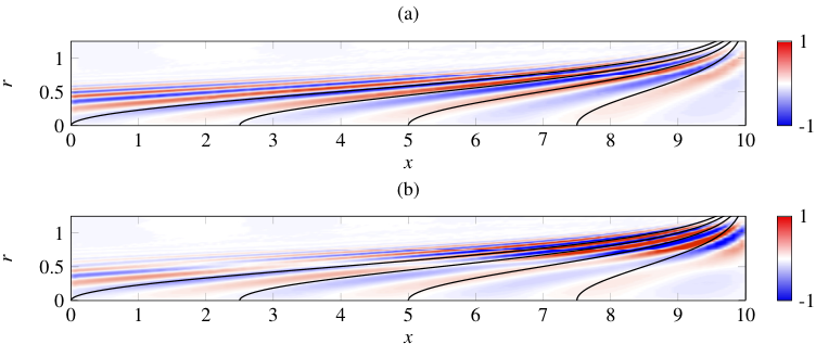
The first two forcing modes are shown in Fig. 10, for a Strouhal number . Tilted structures are observed, quite similar to the compressible results displayed in Fig. 7(a,c), and the tilting angle increases with upstream distance from the target position . Black curves trace material lines in the flow that are transported, through convection with the local flow velocity, into vertical lines at after various time lapses. It is immediately seen that the forcing structures follow closely the local curvature of these contours, especially at far upstream positions. Along the black curves, the phase of the first forcing mode structure is approximately constant, whereas the second mode displays a sign change in the phase at the inflection point . This radial sign change provides for the orthogonality between different forcing modes, and their associated flow responses, while the streamwise variations in modes 1 and 2 are nearly identical. The third and fourth forcing modes of the parallel incompressible jet, not shown in Fig. 10, are merely characterised by additional phase changes in the radial direction. All these features are fully consistent with the sub-optimal forcing structures found for the non-parallel compressible jet (Fig. 7). The parallel jet results clearly demonstrate that an Orr-type convection mechanism is responsible for the forcing gain in this locally stable setting. From their resemblance, it is inferred that the same mechanism accounts for the gain of sub-optimal structures in the non-parallel compressible jet.
In summary, the following main interpretations of the findings in Sec. III.5 are proposed: (i) The optimal forcing (mode 1) targets the shear instability of the jet, leading to exponential amplitude growth along in a finite region directly downstream of the nozzle. Forcing of this mechanism is most efficient at the upstream end of the locally unstable region. Even more efficient than direct forcing of shear-instability perturbations at the nozzle lip is the forcing of Orr structures in the inner pipe boundary layer, which experience growth before they enter the free jet (consistent with Garnaud et al. 2013a; Garnaud et al. 2013b; Semeraro et al. 2016a). (ii) Sub-optimal forcing exploits the Orr mechanism in the free jet as a means of perturbation energy growth, independent of modal shear instability. Successive sub-optimal modes exhibit an increasing number of sign changes in the phase along , which accounts for their mutual orthogonality. (iii) In our present results (Sec. III.5), the above two mechanisms appear to be well separated in the optimal and sub-optimal resolvent modes at moderate Strouhal numbers. At , the shape of the optimal mode (figures 5 and 6) suggests a mixed excitation of shear instability and free-jet Orr mechanism.
V Coherent structures in jet turbulence: experiment and linear model
The resolvent analysis of Sec. III so far only describes the linear flow response to harmonic forcing input. In this section, those results will be leveraged for the modelling of coherent turbulent structures, where both the forcing and the response are of a stochastic nature.
V.1 Extraction of SPOD modes from experimental data


The jet experiments of Jaunet et al. Jaunet et al. 2017 provide an extensive database of synchronous PIV measurements in cross-planes at several axial positions. Two-point coherence statistics along fixed radial positions have been discussed in the first publication Jaunet et al. 2017 with a focus on the streamwise coherence length; here, the same database is fully exploited for the computation of the two-dimensional cross-spectral density of axisymmetric velocity fluctuations in the plane. To our knowledge, no experimental CSD measurements of comparable size and detail in a turbulent jet exist in the literature.
The acquisition apparatus consists of two time-resolved stereo PIV systems that can be moved independently. Both systems measure the velocity in planes orthogonal to the jet axis at either the same axial location (co-planar configuration) or at different positions. A sketch of the setup is shown in Fig. 11, where it is illustrated how the two PIV systems can be positioned with respect to the nozzle. The axial positions of the measurement planes are and in increments of , where refers to the axial position of the upstream system () and to that of the downstream system (). The instantaneous velocity fields are interpolated onto a polar grid of 32 points in the radial direction and 64 in azimuth, for , using a bi-cubic interpolation that guarantees a close match with the original data.
The axisymmetric component of axial velocity fluctuations is isolated by averaging each snapshot in the azimuthal direction. The cross-spectral density (CSD) matrix between all resulting spatial positions is then constructed using Welch’s periodogram method, with data blocks of 128 time samples, overlapped by 50% (see Ref. Jaunet et al. 2017 for further details). This empirically constructed matrix converges statistically towards the true CSD, which is defined as the covariance of the Fourier-transformed velocity signal ,
| (14) |
The ‘expected value’ operator denotes the asymptotic limit of an ensemble average. In the present calculations, for numerical reasons, each element of the CSD matrix is further scaled with a factor , composed of the radial coordinates of any two points for which the correlation is computed. This procedure ensures that the resulting modified CSD matrix is strictly Hermitian Citriniti and George 2000.
Eigenvectors of the modified matrix are computed. These are then again rescaled in each point as , and they are sorted in descending order of their associated eigenvalues. The structures represent the SPOD modes, in the terminology of Picard & Delville Picard and Delville 2000, and as used in recent literature Towne et al. 2018; Schmidt et al. 2018. Unfortunately, the same name is also used by Sieber et al. Sieber et al. 2016 for a different modal decomposition, which is not employed here.
The statistical convergence of SPOD modes is examined by dividing the datasets into two blocks, indicated as , and performing the computation procedure on each subset. Each block corresponds to half of the original dataset. We use a normalised scalar product between each mode obtained with half of the original dataset and the corresponding mode obtained with the complete set,
| (15) |
The scalar quantity is the correlation coefficient between the mode of subset and the corresponding mode of the full dataset. We consider modes with a correlation coefficient close to unity as being converged, showing thus that the same computation with half of the dataset leads to a very similar result.
The correlation coefficients for and 0.8 are presented in Fig. 12. It is clear from these figures that the analysis is rather sensitive to the amount of data being used. The discrepancies in the higher (less energetic) modes are partially explained by differences in the order in which they emerge, depending on the data subset. However, the first two SPOD modes seem to be sufficiently correlated and can be accepted as being converged at all Strouhal numbers below . Only modes 1 and 2 will be discussed in the following, for .
V.2 Resolvent-based modelling of SPOD modes
The relation between resolvent modes, as presented in Sec. III, and SPOD modes, as obtained from the experiments, is made explicit here on the basis of our earlier formulation Semeraro et al. 2016b. The following development is consistent with the recent work of Towne et al. Towne et al. 2018 and Schmidt et al. Schmidt et al. 2018, while using the nomenclature introduced in the previous sections.
Let and represent spatial discretisations of the stochastic forcing and response, as discussed in Sec. III.2. The CSD of their spectral components and is given by
| (16) |
For the purpose of flow modelling, we consider the CSD of an experimentally observable vector of flow quantities,
| (17) |
The relation between and at a given frequency involves the resolvent operator; with (11b) and the definitions in Sec. III.3, this relation can be written as
| (18) |
If the forcing is expanded in the basis given by the columns of , with a coefficient vector such that , (18) becomes
| (19) |
We now seek the relation between eigenvectors (SPOD modes) of and the resolvent response modes contained in the matrix . If full-state information is available, and , one can write
| (20) |
Recall that the scalar product (8) is represented by the matrix . As is unitary, , it represents the eigenvector matrix of , under the condition that is a diagonal matrix. This condition signifies that the resolvent forcing modes, for a given frequency, are uncorrelated in the actual stochastic forcing of the system (‘spatial white-noise hypothesis’). It finally follows that in this case is the eigenvector matrix of (the ‘weighted CSD’ Schmidt et al. 2018), with the diagonal elements of as associated eigenvalues.
If represents only partial-state information, , such a direct link between resolvent response modes and SPOD modes cannot be made. This is the case for the present experimental dataset. However, under the strong hypothesis , it is possible to construct a low-rank approximation
| (21) |
of the observable CSD, where and only contain a limited number of resolvent response modes and associated gains, as obtained from the linear analysis. The eigenvectors of (21), or equivalently the left singular vectors of , can then be identified and compared to those computed from the experimental data. It may be expected that the leading SPOD mode structure is well represented by such a linear model in situations where the first optimal gain is significantly larger than : as the ratio tends towards infinity, the leading SPOD mode tends towards the optimal resolvent response mode . At finite gain ratios however, the inclusion of several resolvent modes in has the potential to improve the agreement. The comparisons provided in recent analyses of backward-facing step flow Beneddine et al. 2016 and jets Towne et al. 2018; Schmidt et al. 2018 show such favourable cases of strong gain separation, as discussed in those articles.
V.3 Comparison between experimental and model results
It is now assessed to what extent the experimentally obtained SPOD modes are accurately reproduced by the resolvent-based model. The success of this comparison depends on many factors, namely, the assumption that our forcing modes are uncorrelated in , the hypotheses involved in the linear resolvent analysis in Sec. III, and the accuracy of both experimental and numerical methods used.
Approximations of are constructed according to the low-rank model (21). The first five resolvent modes, discussed in Sec. III.5, are used to build and (the low-rank versions of and ) at various Strouhal numbers. The matrix selects the streamwise velocity component in the same grid points that are used in the experimental CSDs. SPOD modes are then computed as the left singular modes of the matrix .


The leading SPOD modes obtained from experimental data and from the resolvent-based model are compared in Fig. 13, for Strouhal numbers , 0.4, 0.6 and 0.7. Contours of their absolute value are shown, and each mode is normalised with respect to its global maximum value. The agreement between experimental (left column) and model results (right column) is remarkably good at Strouhal numbers between 0.4 and 0.7. Within this range of , maximum SPOD amplitudes are located inside the potential core region of the jet. The maximum along at each streamwise station follows a line that tends towards the jet axis, evocative of the ‘critical layer’ as discussed by Tissot et al. Tissot et al. 2017a. At however, the agreement between experiment and model is rather poor. While the experimental mode structure in Fig. 13 resembles those found at higher Strouhal numbers, but with its maximum further downstream and possibly outside the measurement window, the resolvent-based model predicts high amplitudes in the outer portion of the shear layer (Figs. 13 and 6).
The second SPOD modes are shown in the same manner in Fig. 14. For these modes, the comparison between experimental and model results fails at all Strouhal numbers. Mode structures obtained from the resolvent-based model have high amplitudes inside the shear layer, similar to the sub-optimal response structures shown in Fig. 7, whereas the experimentally educed structures are still characterised by maximum amplitudes near the jet axis. Inside the jet, the latter display an amplitude modulation along with two distinct local maxima. Subsequent SPOD modes show similarly poor agreement, and they are not reported here.
Several effects may contribute to the failure of the model to capture the second SPOD mode; a rather obvious one seems to derive from the specific structure of the sub-optimal resolvent modes that are included in the low-rank operator (21). The optimal resolvent mode cannot be significantly involved in the second SPOD mode, which is orthogonal to the first one, and none of the four sub-optimal structures in Fig. 7 can be expected to reproduce spatial variations of the kind observed in the left column of Fig. 14.
Energy spectra, as given by the eigenvalues of the measured and modelled CSD matrices, are compared in Fig. 15. Their variations with Strouhal number are quite different from one another. The dominant eigenvalue of the experimental CSD takes on its highest value at , and another local maximum arises at . The first and second eigenvalue curves are separated by a factor between 3 and 7 over the interval , where SPOD modes in model and experiment are in good agreement. CSD eigenvalues derived from the model closely resemble the gain values shown in Fig. 4, with a slight shift of the maximum value from to 0.6. An important source of discrepancy between the dominant branches in figures 15 and is very likely the assumption that all resolvent forcing modes over all Strouhal numbers are contained in the Reynolds stress fluctuations with equal amplitude.

In order to visualise the wavepacket structure of the leading SPOD mode at , the dominant value according to the experimental spectrum (Fig. 15a), the amplitude and the phase of this mode are interpolated onto a fine mesh. This is done both for the experimental and for the model SPOD mode, and the resulting real parts are shown in Fig. 16. Clean wavepackets are recovered, and their resemblance is even more appreciable than in the amplitude plots of Fig. 13. Recall that the model SPOD mode has been obtained as the eigenmode of a CSD matrix that was constructed from the first five resolvent response modes at . The optimal response mode alone is plotted in Fig. 16; although not strictly identical, it is indeed virtually indistinguishable from the five-mode model result. This comparison demonstrates that the extra effort of including sub-optimal response modes in the model has not led to any improvement of the SPOD prediction: the ‘rank 1 approximation’ used in previous studies Beneddine et al. 2016; Schmidt et al. 2018, which consists in equating the optimal response with the first SPOD mode, is applicable in the current jet case, and sub-optimal modes are of no use for increasing the accuracy of the linear model.
For a more quantitative comparison, real-part oscillations of the interpolated SPOD modes are extracted along the centreline, and displayed in Fig. 17, together with their amplitude envelope. Black and red lines represent the five-mode model and the experimental data, respectively. Markers indicate the values obtained directly in the original measurement points. Experimental wavepackets are traced with their actual absolute amplitude, whereas a best-fit coefficient has been constructed, based on the interval , for a proper scaling of the model amplitude. Good agreement is generally observed in the upstream region of exponential amplitude growth; at , the agreement is excellent down to the amplitude maximum. At lower Strouhal numbers, the model underpredicts the maximum, even by a large measure in the case of , whereas at higher Strouhal numbers, the amplitude maximum is overpredicted. Considering that a phase match is imposed in the very first position, , and differences therefore accumulate in the downstream direction, the phase prediction can be said to be satisfactory for all Strouhal numbers above . Several radial positions have been tested for the present comparison, and all have been found to give very similar agreement. The most notable difference between model and experimental results, at , is an underpredicted downstream attenuation of fluctuation amplitudes. This trend is clearly visible in Figs. 13, 16 and 17, and it increases with .
It must be kept in mind that individual wavepackets in the present approach are regarded as isolated objects, which is made possible by our choice to replace the nonlinear term with a generic white noise forcing. In reality, all frequencies and azimuthal wavenumbers are coupled through the nonlinear Reynolds stresses, such that energy is exchanged between coherent structures, axisymmetric and non-axisymmetric, at different frequencies. This energy transfer would be correctly represented by spatial variations of the forcing at a given Strouhal number, which influence the wavepacket envelope, while furthermore the forcing distributions at all Strouhal numbers are coupled among each other. It remains a challenge for future work to identify a consistent way to model these interactions in a turbulent flow with a broadband spectrum of frequencies and azimuthal wavenumbers.
V.4 Comparison with linear jet studies in the recent literature
The resolvent modes presented in Sec. III.5 and their comparison with SPOD modes in Sec. V.3 are, by and large, consistent with the findings of similar recent studies Garnaud et al. 2013a; Jeun et al. 2016; Semeraro et al. 2016a; Towne et al. 2018; Schmidt et al. 2018. One striking difference with the results of Schmidt et al. Schmidt et al. 2018 is noted in the structure of sub-optimal response modes: at Strouhal numbers above 0.2, our computations yield a clean separation between modal shear and non-modal Orr structures, whereas Schmidt et al. Schmidt et al. 2018 observe a mixing of shear-induced wavepackets with Orr-related structures in all their sub-optimals. The associated forcing structures, shown in Figs. 5 and 7, suggest that this difference can be attributed to the presence of a nozzle in our numerical configuration. Forcing inside the pipe is found to be particularly efficient, especially in the case of the optimal resolvent mode, which must therefore be expected to be very sensitive to the truncation of the most receptive flow region. In turn, changes in the optimal mode will be accompanied by changes in the orthogonal sub-optimals. The localisation of optimal forcing in the present results may furthermore be linked to the observed sensitivity of LES statistics with respect to flow details in the nozzle boundary layer Brès et al. 2018.
Numerous previous studies addressing the linear modelling of wavepackets in turbulent jets, when only boundary forcing at the inflow was considered, observed discrepancies in the initial amplitude growth at low Strouhal numbers, typically Gudmundsson and Colonius 2011; Cavalieri et al. 2013; Breakey et al. 2013, which play an important role in the generation of jet noise. These differences were initially attributed either to the weakly non-parallel assumption that underlies the parabolised stability equations (PSE), or to unmodelled nonlinear effects. The limitation of PSE with regard to non-parallelism has since been ruled out by computations based on the fully non-parallel, linearised Euler equations Baqui et al. 2015. We complete this study by revisiting the low-Strouhal discrepancy in the resolvent framework, where volume forcing is included as a surrogate for nonlinear effects.
Figure 18 compares the PSE and measured power-spectral density (PSD) results from Cavalieri et al. Cavalieri et al. 2013 with the kinetic energy of the optimal response modes presented in Sec. III.5. All curves are extracted on the jet axis. It can be seen how, at , the resolvent mode captures the initial wavepacket growth measured in the experiment, and underpredicted by PSE, while at higher Strouhal numbers the PSE solution and resolvent mode comprise similar initial growth. The optimal forcing at (Fig. 5a,b) involves significant contributions from inside the shear layer of the free jet, which were excluded in the models of Refs. Gudmundsson and Colonius 2011; Cavalieri et al. 2013; Breakey et al. 2013; Baqui et al. 2015. This volume forcing boosts the spatial growth of the response wavepacket near the nozzle. Although the high-amplitude portion of the optimal response mode is not in agreement with the experimental PSD, the initial growth is faithfully reproduced. This observation suggests that Orr-type forcing through Reynolds stresses in the free shear layer indeed contributes to perturbation growth at low Strouhal number near the nozzle.
Another much-discussed discrepancy between PSE and PSD results arises in the downstream region where linear models predict a decay in perturbation amplitude, whereas the PSD displays a marked additional growth, accompanied by a slope break in the growth rate. Jordan et al. Jordan et al. 2017 interpret the PSD growth in this region in terms of the non-normality of decaying local eigenmodes. However, this peculiar behaviour of the PSD is entirely absent in the present SPOD results, in agreement with the LES-based analysis by Schmidt et al. Schmidt et al. 2018. This leads us to conclude that the spatio-temporal coherence, from which SPOD modes are derived, provides a sharper and more pertinent criterion for the eduction of coherent turbulent structures than the PSD, which only measures temporal coherence. As discussed by Towne et al. Towne et al. 2018, the PSD may contain the trace of many SPOD modes. Figure 18 strongly suggests that sub-optimal SPOD or resolvent mode wavepackets contribute in a very significant way to the turbulent dynamics downstream of . The Orr-type character of our sub-optimal resolvent modes is fully consistent with the discussion of the PSD behaviour by Tissot et al. Tissot et al. 2017a.
VI Conclusions
Perturbation wavepackets in the mean flow of a turbulent jet have been computed in the form of resolvent modes. Nonlinear terms in the governing equations, which arise in the form of generalised Reynolds stresses, are regarded as generic forcing terms Farrell and Ioannou 1996; McKeon and Sharma 2010; Beneddine et al. 2016. The five leading orthogonal forcing/response modes have been identified for several values of the Strouhal number between 0.2 and 1.5. The most amplified (‘optimal’) mode, over the interval , bears the traits of a shear instability in the free jet, with strong spatial growth in the potential core. This mode arises principally from forcing in the nozzle boundary layer, which takes the shape of tilted structures indicative of the Orr mechanism, as described in our earlier studies Garnaud et al. 2013a; Semeraro et al. 2016a. The dominant role of shear instability in the free-jet portion of the optimal resolvent mode has been demonstrated by projecting the response wavepacket onto a local shear instability mode. Subsequent (‘sub-optimal’) modes, with significantly lower energy gain, appear to exploit the Orr mechanism in the free jet. This interpretation is supported via an analogy with optimal forcing in a fully developed parallel jet. At low Strouhal number, , both shear and Orr mechanisms in the free jet seem to contribute to the optimal resolvent mode in a mixed fashion.
Coherent structures have then been extracted from experimental measurements, in the form of eigenvectors of the cross-spectral density, named ‘spectral POD’ (SPOD) modes Picard and Delville 2000; Towne et al. 2018. Following recent works Semeraro et al. 2016b; Towne et al. 2018, it has been demonstrated that such modes should, in theory, correspond to the optimal response mode described above, under two strong conditions: (i) the corresponding optimal forcing modes are statistically uncorrelated among each other in the nonlinear dynamics, which are interpreted in the linear model as forcing terms; (ii) the SPOD modes are extracted from full-state information. As full-state information is not available from the experimental dataset, the five leading response modes were instead used to construct a low-rank model of the cross-spectral density, under the even stronger assumption that the corresponding optimal forcing structures are uncorrelated and of equal amplitude in the nonlinear dynamics. This procedure constitutes our resolvent-based linear model for the statistical dynamics of coherent turbulence structures, as characterised by two-point covariance.
Very good agreement has been found between the leading SPOD modes as obtained from the experiment and from the resolvent-based model, in a range of Strouhal numbers around 0.4. The leading SPOD mode of the linear model is in fact nearly identical to the optimal response wavepacket, such that the intermediate step of building a model CSD from several response structures turned out to be unimportant for the comparison with the experiment. At , the model reproduces accurately both the amplitude variations over three decades, down to at least 7 diameters behind the nozzle, and the phase variations in the extracted educed SPOD mode. The maximum wavepacket amplitude is underpredicted at , and overpredicted at . At all Strouhal numbers between 0.2 and 0.7, the initial streamwise perturbation growth close to the nozzle is very well retrieved.
Subsequent (non-leading) SPOD modes of the experimental data and the linear model do not show satisfactory agreement. The discussion of their discrepancies may be approached from two ends: on the one hand, the linear model probably cannot replicate the experimental results because of the restricted number of basis vectors, and because the above-mentioned modelling hypotheses are too crude in order to reproduce the dynamics beyond leading order. On the other hand, the experimental measurements may be too sparse, particularly in terms of spatial resolution, in order to detect the rather fine-scale structures that the linear model predicts.
In summary, the results presented in this paper demonstrate that linear resolvent analysis, performed around the spatially developing, time-averaged mean flow, represents a valid tool for the modelling of coherent wavepacket structures in a stochastically driven turbulent jet. Only the mean flow is required for the construction of this linear model. Wavepackets arising from shear instability, which experience the strongest energy gain, could be matched between model and experiment at Strouhal numbers between 0.2 and 0.7. While these general conclusions corroborate those of the parallel study by Schmidt et al. Schmidt et al. 2018, performed on the basis of LES data for the same flow configuration, differences are observed in the resolvent mode structures. These relate to the separation of shear and Orr mechanisms in the optimal and sub-optimal modes, and they are attributed to the inclusion of a nozzle in the present analysis.
From a final comparison with earlier PSD measurements Cavalieri et al. 2013, it is inferred that sub-optimal SPOD modes seem to play a determining role near and beyond the end of the potential core region. While the link between these modes and free-jet Orr-type growth mechanisms is one more time predicted by the present analysis, poor agreement is found between sub-optimal structures in model and experiment. Further progress of wavepacket modelling in high Reynolds number turbulent jets requires establishing the dynamics that dominate in the flow region downstream of the potential core, and how best to model them.
Acknowledgements.
This work was supported by the Agence Nationale de la Recherche under the Cool Jazz project, grant number ANR-12-BS09-0024, and by the Délégation Générale de l’Armement under grant number 2015.60.0004.00.470.75.01. Stability calculations were performed using HPC resources of TGCC and CINES under the allocation x2016-2a6451 made by GENCI.References
- Jordan and Colonius (2013) P. Jordan and T. Colonius, “Wave packets and turbulent jet noise,” Annu. Rev. Fluid Mech. 45, 173–195 (2013).
- Michalke (1971) A. Michalke, “Instabilität eines kompressiblen runden Freistrahls unter Berücksichtigung des Einflusses der Strahlgrenzschichtdicke,” Z. Flugwiss. 19, 319–328 (1971).
- Crighton and Gaster (1976) D. G. Crighton and M. Gaster, “Stability of slowly diverging jet flow,” J. Fluid Mech. 77, 397–413 (1976).
- Oberleithner et al. (2014) K. Oberleithner, L. Rukes, and J. Soria, “Mean flow stability analysis of oscillating jet experiments,” J. Fluid Mech. 757, 1–32 (2014).
- Gudmundsson and Colonius (2011) K. Gudmundsson and T. Colonius, “Instability wave models for the near-field fluctuations of turbulent jets,” J. Fluid Mech. 689, 97–128 (2011).
- Baqui et al. (2015) Y. B. Baqui, A. Agarwal, A. V. G. Cavalieri, and S. Sinayoko, “A coherence-matched linear source mechanism for subsonic jet noise,” J. Fluid Mech. 776, 235–267 (2015).
- Farrell and Ioannou (1993) B. F. Farrell and P. J. Ioannou, “Stochastic forcing of the linearized Navier–Stokes equations,” Phys. Fluids A 5, 2600–2609 (1993).
- Farrell and Ioannou (2014) B. F. Farrell and P. J. Ioannou, “Statistical state dynamics: a new perspective on turbulence in shear flow,” arXiv preprint 1412.8290 (2014).
- Schmid (2007) P. J. Schmid, “Nonmodal stability theory,” Annu. Rev. Fluid Mech. 39, 129–162 (2007).
- Bagheri et al. (2009) S. Bagheri, D. S. Henningson, J. Hoepffner, and P. J. Schmid, “Input-output analysis and control design applied to a linear model of spatially developing flows,” Appl. Mech. Rev. 62, 020803 (2009).
- Picard and Delville (2000) C. Picard and J. Delville, “Pressure velocity coupling in a subsonic round jet,” Int. J. Heat Fluid Fl. 21, 359–364 (2000).
- Sieber et al. (2016) M. Sieber, C. O. Paschereit, and K. Oberleithner, “Spectral proper orthogonal decomposition,” J. Fluid Mech. 792, 798–828 (2016).
- Cavalieri et al. (2013) A. V. G. Cavalieri, D. Rodriguez, P. Jordan, T. Colonius, and Y. Gervais, “Wavepackets in the velocity field of turbulent jets,” J. Fluid Mech. 730, 559–592 (2013).
- Rodriguez et al. (2015) D. Rodriguez, A. V. G. Cavalieri, T. Colonius, and P. Jordan, “A study of linear wavepacket models for subsonic turbulent jets using local eigenmode decomposition of PIV data,” Eur. J. Mech. B/Fluids 49B, 308–321 (2015).
- Garnaud et al. (2013a) X. Garnaud, L. Lesshafft, P. J. Schmid, and P. Huerre, “The preferred mode of incompressible jets: linear frequency response analysis,” J. Fluid Mech. 716, 189–202 (2013a).
- Garnaud et al. (2013b) X. Garnaud, R. D. Sandberg, and L. Lesshafft, “Global response to forcing in a subsonic jet: instability wavepackets and acoustic radiation,” AIAA Paper 2013–4633 (2013b).
- Jeun et al. (2016) J. Jeun, J. W. Nichols, and M. R. Jovanović, “Input-output analysis of high-speed axisymmetric isothermal jet noise,” Phys. Fluids 28, 047101 (2016).
- Semeraro et al. (2016a) O. Semeraro, L. Lesshafft, V. Jaunet, and P. Jordan, “Modeling of coherent structures in a turbulent jet as global linear instability wavepackets: Theory and experiment,” Int. J. Heat Fluid Fl. 62, 24–32 (2016a).
- Semeraro et al. (2016b) O. Semeraro, V. Jaunet, P. Jordan, A. V. G. Cavalieri, and L. Lesshafft, “Stochastic and harmonic optimal forcing in subsonic jets,” AIAA Paper 2016-2935 (2016b).
- Towne et al. (2018) A. Towne, O. T. Schmidt, and T. Colonius, “Spectral proper orthogonal decomposition and its relationship to dynamic mode decomposition and resolvent analysis,” J. Fluid Mech. 847, 821–867 (2018).
- Schmidt et al. (2018) O. T. Schmidt, A. Towne, G. Rigas, T. Colonius, and G. A. Brès, “Spectral analysis of jet turbulence,” J. Fluid Mech. 855, 953–982 (2018).
- Farrell and Ioannou (1996) B. F. Farrell and P. J. Ioannou, “Generalized stability theory. Part I: Autonomous operators,” J. Atmospheric Sci. 53, 2025–2040 (1996).
- Alizard et al. (2009) F. Alizard, S. Cherubini, and J.-C. Robinet, “Sensitivity and optimal forcing response in separated boundary layer flows,” Phys. Fluids 21, 064108 (2009).
- Monokrousos et al. (2010) A. Monokrousos, E. Åkervik, L. Brandt, and D. S. Henningson, “Global three-dimensional optimal disturbances in the Blasius boundary-layer flow using time-steppers,” J. Fluid Mech. 650, 181–214 (2010).
- Sipp and Marquet (2013) D. Sipp and O. Marquet, “Characterization of noise amplifiers with global singular modes: the case of the leading-edge flat-plate boundary layer,” Theor. Comp. Fluid Dyn. 27, 617–635 (2013).
- Dergham et al. (2013) G. Dergham, D. Sipp, and J.-C. Robinet, “Stochastic dynamics and model reduction of amplifier flows: the backward facing step flow,” J. Fluid Mech. 719, 406–430 (2013).
- Boujo and Gallaire (2015) E. Boujo and F. Gallaire, “Sensitivity and open-loop control of stochastic response in a noise amplifier flow: the backward-facing step,” J. Fluid Mech. 762, 361–392 (2015).
- Beneddine et al. (2016) S. Beneddine, D. Sipp, A. Arnault, J. Dandois, and L. Lesshafft, “Conditions for validity of mean flow stability analysis,” J. Fluid Mech. 798, 485–504 (2016).
- Towne et al. (2015) A. Towne, T. Colonius, P. Jordan, A. V. G. Cavalieri, and G. A. Brès, “Stochastic and nonlinear forcing of wavepackets in a Mach 0.9 jet,” AIAA Paper 2015-2217 (2015).
- Cavalieri et al. (2019) A. V. G. Cavalieri, P. Jordan, and L. Lesshafft, “Wave-packet models for jet dynamics and sound radiation,” Appl. Mech. Rev. (2019), doi:10.1115/1.4042736.
- Jaunet et al. (2017) V. Jaunet, P. Jordan, and A. V. G. Cavalieri, “Two-point coherence of wave packets in turbulent jets,” Phys. Rev. Fluids 2, 024604 (2017).
- Brès et al. (2018) G. A. Brès, P. Jordan, V. Jaunet, M. Le Rallic, A. V. G. Cavalieri, A. Towne, S. K. Lele, T. Colonius, and O. T. Schmidt, “Importance of the nozzle-exit boundary-layer state in subsonic turbulent jets,” J. Fluid Mech. 851, 83–124 (2018).
- (33) See Supplemental Material at [URL will be inserted by publisher] for the mean flow file.
- Pope (2000) S. B. Pope, Turbulent flows (Cambridge University Press, 2000).
- Garnaud (2012) X. Garnaud, Modes, transient dynamics and forced response of circular jets, Ph.D. thesis, Ecole polytechnique, Palaiseau, France (2012).
- Sandberg (2007) R. D. Sandberg, “Governing equations for a new compressible Navier-Stokes solver in general cylindrical coordinates,” Monograph No. AFM-07/07, School of Engineering Sciences, University of Southampton (2007).
- Reynolds and Hussain (1972) W. C. Reynolds and A. K. M. F. Hussain, “The mechanics of an organized wave in turbulent shear flow. Part 3. Theoretical models and comparisons with experiments,” J. Fluid Mech. 54, 263–288 (1972).
- McKeon and Sharma (2010) B. J. McKeon and A. S. Sharma, “A critical-layer framework for turbulent pipe flow,” J. Fluid Mech. 658, 336–382 (2010).
- Tammisola and Juniper (2016) O. Tammisola and M. P. Juniper, “Coherent structures in a swirl injector at Re=4800 by nonlinear simulations and linear global modes,” J. Fluid Mech. 792, 620–657 (2016).
- Oberleithner et al. (2015) K. Oberleithner, M. Stöhr, S. H. Im, C. M. Arndt, and A. M. Steinberg, “Formation and flame-induced suppression of the precessing vortex core in a swirl combustor: experiments and linear stability analysis,” Combust. Flame 162, 3100–3114 (2015).
- Semeraro et al. (2016c) O. Semeraro, L. Lesshafft, and R. D. Sandberg, “Can jet noise be predicted using linear instability wavepackets?” in Proceedings of the 5th International Conference on Jets, Wakes and Separated Flows (Springer, 2016) pp. 413–418.
- Åkervik et al. (2008) E. Åkervik, U. Ehrenstein, F. Gallaire, and D. S. Henningson, “Global two-dimensional stability measures of the flat plate boundary-layer flow,” Eur. J. Mech. B/Fluids 27, 501–513 (2008).
- Huerre and Monkewitz (1990) P. Huerre and P. Monkewitz, “Local and global instabilities in spatially developing flows,” Annu. Rev. Fluid Mech. 22, 473–537 (1990).
- Garnaud et al. (2013c) X. Garnaud, L. Lesshafft, P. J. Schmid, and P. Huerre, “Modal and transient dynamics of jet flows,” Phys. Fluids 25, 044103 (2013c).
- Chu (1965) B.-T. Chu, “On the energy transfer to small disturbances in fluid flow (Part I),” Acta Mech. 1, 215–234 (1965).
- Hernandez et al. (2005) V. Hernandez, J. E. Roman, and V. Vidal, “SLEPc: A scalable and flexible toolkit for the solution of eigenvalue problems,” ACM Transactions on Mathematical Software (TOMS) 31, 351–362 (2005).
- Fosas de Pando et al. (2012) M. Fosas de Pando, D. Sipp, and P. J. Schmid, “Efficient evaluation of the direct and adjoint linearized dynamics from compressible flow solvers,” J. Comput. Phys. 231, 7739–7755 (2012).
- Berland et al. (2007) J. Berland, C. Bogey, O. Marsden, and C. Bailly, “High-order, low dispersive and low dissipative explicit schemes for multiple-scale and boundary problems,” J. Comput. Phys. 224, 637–662 (2007).
- Poinsot and Lele (1992) T. J. Poinsot and S. K. Lele, “Boundary conditions for direct simulations of compressible viscous flows,” J. Comput. Phys. 101, 104–129 (1992).
- Colonius (2004) T. Colonius, “Modeling artificial boundary conditions for compressible flow,” Annu. Rev. Fluid Mech. 36, 315–345 (2004).
- Tissot et al. (2017a) G. Tissot, M. Zhang, F. Lajus, A. V. G. Cavalieri, P. Jordan, and T. Colonius, “Sensitivity of wavepackets in jets to non-linear effects: the role of the critical layer,” J. Fluid Mech. 811, 95–137 (2017a).
- Tissot et al. (2017b) G. Tissot, F. Lajús, A. V. G. Cavalieri, and P. Jordan, “Wave packets and Orr mechanism in turbulent jets,” Phys. Rev. Fluids 2, 093901 (2017b).
- Butler and Farrell (1992) K. M. Butler and B. F. Farrell, “Three-dimensional optimal perturbations in viscous shear flow,” Phys. Fluids A 4, 1637–1650 (1992).
- Jiménez (2013) J. Jiménez, “How linear is wall-bounded turbulence?” Phys. Fluids 25, 110814 (2013).
- Lesshafft and Huerre (2007) L. Lesshafft and P. Huerre, “Linear impulse response in hot round jets,” Phys. Fluids 19, 024102 (2007).
- Le Dizès et al. (1995) S. Le Dizès, P. A. Monkewitz, and P. Huerre, “Viscous structure of plane waves in spatially developing shear flows,” Phys. Fluids 7, 1337–1347 (1995).
- Lesshafft (2018) L. Lesshafft, “Artificial eigenmodes in truncated flow domains,” Theor. Comput. Fluid Dyn. 32, 245–262 (2018).
- Citriniti and George (2000) J. H. Citriniti and W. K. George, “Reconstruction of the global velocity field in the axisymmetric mixing layer utilizing the proper orthogonal decomposition,” J. Fluid Mech. 418, 137–166 (2000).
- Breakey et al. (2013) D. E. Breakey, P. Jordan, A. V. G. Cavalieri, and O. Léon, “Near-field wavepackets and the far-field sound of a subsonic jet,” AIAA Paper 2013-2083 (2013).
- Jordan et al. (2017) P. Jordan, M. Zhang, G. Lehnasch, and A. V. G. Cavalieri, “Modal and non-modal linear wavepacket dynamics in turbulent jets,” AIAA Paper 2017-3379 (2017).