跳到论文正文
W Papers独立论文阅读器 arXiv:1810.09298 论文正文 计算阅读时间 · 0%
引用这篇论文根据当前论文元数据生成,正式投稿前建议核对。


License: arXiv.org perpetual non-exclusive license
arXiv:1810.09298v2 [stat.ME] 23 Nov 2018

Sparse constrained projection approximation subspace tracking

Denis Belomestny    Ekaterina Krymova Thanks: The authors are with Faculty of Mathematics at the University Duisburg-Essen, Essen, Germany Thanks: D. Belomestny e-mail: denis.belomestny@uni-due.de Thanks: E. Krymova e-mail: ekaterina.krymova@uni-due.de Thanks: This work is funded by the German Research Foundation (DFG), Collaborative Research Center 823, Subprojects B3 and C5. The first author was also supported by the RSF grant 18-11-00132
Abstract

In this paper we revisit the well-known constrained projection approximation subspace tracking algorithm (CPAST) and derive, for the first time, non-asymptotic error bounds. Furthermore, we introduce a novel sparse modification of CPAST which is able to exploit sparsity in the underlying covariance structure. We present a non-asymptotic analysis of the proposed algorithm and study its empirical performance on simulated and real data.

1 Introduction

Subspace tracking methods are intensively used in statistical and signal processing community. Given observations of a multidimensional signal, one is interested in estimating or tracking a subspace spanning the eigenvectors corresponding to the first largest eigenvalues of the signal covariance matrix. Over the past few decades many variations of the original projection approximation subspace tracking (PAST) method [1] were developed which found applications in data compression, filtering, speech enhancement, etc. (see [2] and references therein). Despite popularity of the subspace tracking methods, only partial results are known about their convergence. The asymptotic convergence of the PAST algorithm was first established in [3, 4] using a general theory of stability for ordinary differential equations. However, no finite sample error bounds are available in the literature. Furthermore, in the case of a high-dimensional signal the empirical covariance matrix estimator performs poorly if the number of observations is small. A common way to improve the estimation quality in this case is to impose some kind of sparsity assumptions on the signal itself or on the eigensubspace of the underlying covariance matrix. In [5] a sparse modification of the orthogonal iteration scheme for a fixed number of observations was proposed. A thorough analysis in [5] shows that under appropriate sparsity assumptions on the leading eigenvectors, the orthogonal iteration scheme combined with thresholding allows to perform dimension reduction in high-dimensional setting. Our main goal is to propose a novel modification of constraint projection approximation subspace tracking method (CPAST) [6], called sparse projection approximation subspace tracking method (SCPAST), which can be used for efficient subspace tracking in the case of high-dimensional sparse signal and small number of available observations. Another contribution of our paper is a non-asymptotic convergence analysis of CPAST and SCPAST algorithms showing the advantage of SCPAST algorithm in the case of sparse covariance structure. Last but not the least, we analyse numerical performance of SCPAST algorithm on simulated and real data. In particular, the problem of tracking the leading subspace of a music signal is considered.

The structure of the paper is as follows. In Section 2 we introduce our observational model and formulate main assumptions. Section 3 first reviews the CPAST algorithm and then provides the non-asymptotic error bounds for CPAST in a ”stationary” case. In Section 4 we introduce our sparse constraint approximation subspace tracking method and prove the non-asymptotic upper bounds for the estimation error. A numerical study of the proposed algorithm is presented in Section 5. Finally the proofs are collected in Section 6.

2 Main setup

One important problem in signal processing is adaptive estimation of a dominant subspace given incoming noisy observations. Specifically one considers a model

x(t)=s(t)+σ(t)ξ(t),t=1,…,T,x(t)=s(t)+\sigma(t)\xi(t),\quad t=1,\dots,T, (1)

where the observations x⁡(t)∈ℝnx(t)\in\mathbb{R}^{n} contain the signal s⁡(t)∈ℝns(t)\in\mathbb{R}^{n} corrupted by a vector ξ⁡(t)∈ℝn\xi(t)\in\mathbb{R}^{n} with independent standard Gaussian components. The signal s⁡(t)s(t) is usually modelled as

s⁡(t)=A⁡(t)​η​(t),s(t)=A(t)\eta(t),

where A⁡(t)A(t) is a deterministic n×dn\times d matrix of rank dd with d≪nd\ll n and η⁡(t)\eta(t) is a random vector in ℝd\mathbb{R}^{d} independent of ξ⁡(t),\xi(t), such that 𝐄⁡[η⁡(t)]=0\mathbf{E}[\eta(t)]=0 and 𝐄⁡[ηi2​(t)]=1\mathbf{E}[\eta_{i}^{2}(t)]=1, i=1,…,di=1,\dots,d. Under these assumptions, the process x⁡(t)x(t) has a covariance matrix Σ⁡(t)\Sigma(t) which may be decomposed in the following way

Σ⁡(t)=𝐄⁡[x⁡(t)​x⊤​(t)]=A⁡(t)​A⊤​(t)+σ2​(t)​In,\Sigma(t)=\mathbf{E}[x(t)x^{\top}(t)]=A(t)A^{\top}(t)+\sigma^{2}(t)I_{n}, (2)

where InI_{n} stands for the unit matrix in ℝn.\mathbb{R}^{n}. Note that the matrix A⁡(t)​A⊤​(t)A(t)A^{\top}(t) has the rank dd and by the singular value decomposition (SVD)

A⁡(t)​A⊤​(t)\displaystyle A(t)A^{\top}(t) =∑i=1dλi​(t)​vi​(t)​vi⊤​(t),\displaystyle=\sum_{i=1}^{d}\lambda_{i}(t)v_{i}(t)v_{i}^{\top}(t),

where vi(t)∈ℝn,i=1,…,d,v_{i}(t)\in\mathbb{R}^{n},\,i=1,\dots,d, are the eigenvectors of A⁡(t)​A⊤​(t)A(t)A^{\top}(t) corresponding to the eigenvalues λ1​(t)≥λ2​(t)≥⋯≥λd​(t)>0\lambda_{1}(t)\geq\lambda_{2}(t)\geq\dots\geq\lambda_{d}(t)>0. It follows from (2) that the first dd eigenvalues of Σ⁡(t)\Sigma(t) are λ1​(t)+σ2​(t),…,λd​(t)+σ2​(t),\lambda_{1}(t)+\sigma^{2}(t),\dots,\lambda_{d}(t)+\sigma^{2}(t), whereas the remaining n−dn-d eigenvalues are equal to σ2​(t)\sigma^{2}(t). Since λd​(t)>0,\lambda_{d}(t)>0, the subspace corresponding to the first dd eigenvectors of A⁡(t)​A⊤​(t)A(t)A^{\top}(t) is identifiable. The subspace tracking methods aim to estimate the subspace span⁡(v1​(t),…,vd​(t))\mathrm{span}(v_{1}(t),\ldots,v_{d}(t)) based on the observations (x⁡(k))k=1t.(x(k))_{k=1}^{t}. The overall number of observations TT is assumed to be fixed and known.

Relying on a heuristic assumption of slow (in time) varying Σ⁡(t)\Sigma(t), the subspace tracking methods use the following estimator of the covariance matrix (up to scaling)

Σ^γ​(t)=∑i=0tγt−i​x​(i)​x⊤​(i),\widehat{\Sigma}_{\gamma}(t)=\sum_{i=0}^{t}\gamma^{t-i}x(i)x^{\top}(i), (3)

where 0<γ≤10<\gamma\leq 1 is the so-called forgetting factor. The estimator Σ^γ​(t)\widehat{\Sigma}_{\gamma}(t) can adapt to the change in Σ⁡(t)\Sigma(t) by discounting the past observations. In the stationary regime, that is, if Σ⁡(t)\Sigma(t) is a constant matrix, one would use γ=1\gamma=1. It is well known, that in the case of Gaussian independent noise the estimator Σ^1​(t)\widehat{\Sigma}_{1}(t) is consistent.

3 CPAST

For the general model (1) and non-stationary case, constrained projection approximation subspace tracking (CPAST) method allows to iteratively compute a matrix V^γ​(t)\widehat{V}_{\gamma}(t), t=1,…,Tt=1,\dots,T, containing the first dd leading eigenvectors of the matrix Σ^γ​(t)\widehat{\Sigma}_{\gamma}(t) (see (3)) based on sequentially arriving observations x⁡(j)x(j), j=1,…,t.j=1,\dots,t. The procedure starts with some initial approximation V^γ​(0)=V^0\widehat{V}_{\gamma}(0)=\widehat{V}^{0} and consists of the following two steps

  • •

    multiplication: compute the n×dn\times d matrix

    Σ^γ,V​(t)=Σ^γ​(t)​V^γ​(t−1);\widehat{\Sigma}_{\gamma,V}(t)=\widehat{\Sigma}_{\gamma}(t)\widehat{V}_{\gamma}(t-1);
  • •

    orthogonalization: compute an estimator V^γ​(t)\widehat{V}_{\gamma}(t) of the matrix V⁡(t)V(t) containing dd leading eigenvectors via

    V^γ(t)=Σ^γ,V(t)[Σ^γ,V⊤(t)Σ^γ,V(t)]−1/2.\widehat{V}_{\gamma}(t)=\widehat{\Sigma}_{\gamma,V}(t)[\widehat{\Sigma}_{\gamma,V}^{\top}(t)\widehat{\Sigma}_{\gamma,V}(t)]^{-1/2}.

In the ”stationary” case (γ=1\gamma=1) the method may be regarded as the ”online”-version of the orthogonal iterations scheme (see [7]) for computing the eigen-subspace of the non-negatively definite matrix. With the use of the Sherman-Morrison-Woodbury formula for the inversion at each time t,t, one has to perform O⁡(n​d2)O(nd^{2}) operations to compute the updated matrix V^γ​(t)\widehat{V}_{\gamma}(t) given V^γ​(t−1)\widehat{V}_{\gamma}(t-1), Σ^γ​(t−1)\widehat{\Sigma}_{\gamma}(t-1) and x⁡(t)x(t).

3.1 Convergence of CPAST

Throughout this section we consider the stationary case where Σ⁡(t)=Σ\Sigma(t)=\Sigma, A⁡(t)=AA(t)=A, vi​(t)=viv_{i}(t)=v_{i}, λi​(t)=λi\lambda_{i}(t)=\lambda_{i}, i=1,…,di=1,\dots,d, σ2​(t)=σ2\sigma^{2}(t)=\sigma^{2}. In this situation one would like to keep all the available information to estimate VV, that is, to use the estimator (3) for Σ\Sigma with γ=1\gamma=1. For notational simplicity, from now on we skip the dependence on γ\gamma and use the notation Σ^​(t)\widehat{\Sigma}(t) for the empirical covariance matrix Σ^​(t)=1t​∑i=1tx⁡(i)​x⊤​(i)\widehat{\Sigma}(t)=\frac{1}{t}\sum_{i=1}^{t}x(i)x^{\top}(i) and V^​(t)\widehat{V}(t) for CPAST estimator. Thus in the stationary case the CPAST estimator takes the form

V^(t)=[Σ^(t)V^(t−1)][V^⊤(t−1)⊤Σ^2(t)V^(t−1)]−1/2.\widehat{V}(t)=[\widehat{\Sigma}(t)\widehat{V}(t-1)][\widehat{V}^{\top}(t-1)^{\top}\widehat{\Sigma}^{2}(t)\widehat{V}(t-1)]^{-1/2}. (4)

We assume that the random vectors η⁡(t)\eta(t) and ξ⁡(t)\xi(t) have independent 𝒩⁡(0,1)\mathcal{N}(0,1) components for t=1,…,Tt=1,\dots,T. Under these assumptions the covariance matrix (2) becomes

Σ=∑i=1dλi​vi​vi⊤+σ2​In=V​Λd​V⊤+σ2​In,\begin{split}\Sigma=\sum_{i=1}^{d}\lambda_{i}v_{i}v_{i}^{\top}+\sigma^{2}I_{n}=V\Lambda_{d}V^{\top}+\sigma^{2}I_{n},\end{split} (5)

where VV is n×dn\times d matrix with columns {vi}i=1d\{v_{i}\}_{i=1}^{d}, Λd\Lambda_{d} is d×dd\times d diagonal matrix with {λi}i=1d\{\lambda_{i}\}_{i=1}^{d} on the diagonal. Note that the observational model (1) in stationary case can be alternatively written as the so-called spike model

x⁡(t)=∑i=1dλi​ui​(t)​vi+σ​ξ​(t),x(t)=\sum_{i=1}^{d}\sqrt{\lambda_{i}}u_{i}(t)v_{i}+\sigma\xi(t), (6)

where ui​(t)u_{i}(t) are i.i.d. standard Gaussian random variables independent from ξ⁡(t)\xi(t).

For our non-asymptotic error analysis of CPAST, we assume that dd, σ2\sigma^{2} and λi\lambda_{i}, i=1,…,di=1,\dots,d are known. With the known σ2\sigma^{2} we can always normalize the data and therefore without loss of generality we can assume that σ2=1\sigma^{2}=1.

The typical condition while analyzing the quality of the eigenvectors estimation is the so-called spectral gap condition, which says that the adjacent eigenvectors explain distinguishably different portion of the variance in the data, namely there exists τ≥1\tau\geq 1, such that for all j=1,…,d,j=1,\dots,d,

τ⁡(λj−λj+1)≥λ1,\tau(\lambda_{j}-\lambda_{j+1})\geq\lambda_{1},

where λd+1=0\lambda_{d+1}=0 by definition. Since our goal is the estimation of the dd-dimensional subspace of the first eigenvectors, and we are not interested in the estimation of each particular eigenvector, we need only the condition for the separation of this dd-dimensional subspace, namely that the gap between λd\lambda_{d} and λd+1\lambda_{d+1} is sufficiently large:

τ​λd≥λ1.\tau\lambda_{d}\geq\lambda_{1}. (7)

Define a distance ll between two subspaces 𝒲\mathcal{W} and 𝒬\mathcal{Q} spanning orthonormal columns w1,…,wdw_{1},\ldots,w_{d} and q1,…,qdq_{1},\ldots,q_{d} correspondingly via

l⁡(W,Q)=l⁡(𝒲,𝒬)=‖W​W⊤−Q​Q⊤‖2,l({W},{Q})=l(\mathcal{W},\mathcal{Q})=\|WW^{\top}-QQ^{\top}\|^{2}, (8)

where the nuclear norm ‖A‖\|A\| of a matrix A∈ℝn×dA\in\mathbb{R}^{n\times d} is defined as ‖A‖=supx∈ℝd‖A​x‖2‖x‖2\|A\|=\sup_{x\in\mathbb{R}^{d}}\frac{\|Ax\|_{2}}{\|x\|_{2}}, and W={w1,…,wd}W=\{w_{1},\dots,w_{d}\} and Q={q1,…,qd}Q=\{q_{1},\dots,q_{d}\} are the matrices in ℝn×d\mathbb{R}^{n\times d} with orthonormal columns.

The next result shows that with high probability the subspace which spans the CPAST estimator V^​(t)\widehat{V}(t) is close, in terms of l,l, to the subspace spanning VV when the number of observation is large enough. We assume that the initial estimator V^​(t0)=V^0\widehat{V}(t_{0})=\widehat{V}^{0} is constructed from t0t_{0} first observations by means of the singular value decomposition of Σ^​(t0)\widehat{\Sigma}(t_{0}).

Theorem 1.

Suppose that the spectral gap condition (7) holds and

t0≥4​2​Rmax​λ1+1λd,\sqrt{t_{0}}\geq 4\sqrt{2}R_{\max}\frac{\lambda_{1}+1}{\lambda_{d}},

where Rmax=5​n−d+5​6​ln⁡(n∨T)R_{\max}=5\sqrt{n-d}+5\sqrt{6}\sqrt{\ln(n\vee T)}. Then after t−t0t-t_{0} iterations we get with probability at least 1−C0​(n∨t)−2,1-{C_{0}}(n\vee t)^{-2},

l​(V,V^​(t))≤C1​λd+1λd2​n−dt+C2​λ1+1λd2​log⁡(n∨t)t,\begin{split}l(V,\widehat{V}(t))\leq&C_{1}\frac{\lambda_{d}+1}{\lambda_{d}^{2}}\frac{n-d}{t}+C_{2}\frac{\lambda_{1}+1}{\lambda_{d}^{2}}\frac{\log(n\vee t)}{t},\end{split} (9)

where C0,C_{0}, C2C_{2} are absolute constants and C1C_{1} depends on τ.\tau.

Remark 1.

The second term on the right-hand side of (9) corresponds to the error of separating the first dd eigenvectors from the rest. The first term is an average error of estimating all components of dd leading eigenvectors. It originates from the interaction of the noise terms with the different coordinates, see [8].

4 Sparse CPAST

4.1 Sparsity assumptions on leading eigenvectors

We assume that in the stationary case (5) the first dd leading eigenvectors viv_{i}, i=1,…,d,i=1,\dots,d, of Σ\Sigma have most of their entries close to zero. Namely, we suppose that each viv_{i} fulfils the so-called weak-lrl_{r} ball condition [9, 10], that is, for some r∈(0,2),r\in(0,2),

|vi|(k)≤sik−1/r,k=1,…,n.|v_{i}|_{(k)}\leq s_{i}k^{-1/r},\quad k=1,\dots,n.

where |vi|(k)|v_{i}|_{(k)} is the kk-th largest coordinate of viv_{i}. The weak-lrl_{r} ball condition is known to be more general than lrl_{r} ball condition (which is ‖q‖r≤s\|q\|_{r}\leq s for q∈ℝnq\in\mathbb{R}^{n}, r∈(0,2)r\in(0,2), s≥1s\geq 1), as it combines different definitions of sparsity used in statistics, see [11].

Define a thresholding function g⁡(x,β)g(x,\beta) with a thresholding parameter β>0\beta>0 and x∈ℝx\in\mathbb{R} via

x−β≤g⁡(x,β)≤x+β,g⁡(x,β)​1|x|≤β=0.x-\beta\leq g(x,\beta)\leq x+\beta,\quad g(x,\beta)1_{|x|\leq\beta}=0. (10)

For example, the so-called hard-thresholding function gH​(x,β)g_{H}(x,\beta) given by

gH​(x,β)=x​1(|x|≤β)g_{H}(x,\beta)=x1_{(|x|\leq\beta)} (11)

and the so-called soft-thresholding function defined as

gS​(x,β)=(x−β)+⋅sign⁡(x)g_{S}(x,\beta)=(x-\beta)_{+}\cdot{\rm sign}(x)

fulfill the conditions (10). When β\beta is a vector with components βi\beta_{i}, i=1,…,di=1,\dots,d, and VV is a matrix with columns vi∈ℝnv_{i}\in\mathbb{R}^{n}, i=1,…,di=1,\dots,d, we denote by g⁡(V,β)g(V,\beta) a n×dn\times d matrix with the elements {g⁡(vi​j,βi)}\{g(v_{ij},\beta_{i})\}, i=1,…,di=1,\dots,d, j=1,…,nj=1,\dots,n.

Our primal goal is to propose a subspace tracking method for estimating a dd-dimensional subspace of the process under weak-lrl_{r} ball assumption on the leading eigenvectors of the covariance matrix Σ\Sigma and to analyze it’s convergence.

4.2 Initialization and main steps

Our sparse modification of CPAST relies on the orthogonal iteration scheme with an additional thresholding step (cf. [5, 10]). From now on, by a slight abuse of notation, we will denote by V^​(t)\widehat{V}(t) an iterative estimator obtained with the help of the modified CPAST, given tt observations. To get the initial approximation V^​(t0),\widehat{V}(t_{0}), we use the following modification of a standard SPCA scheme, see [5, 10].

  1. 1.

    First compute the empirical covariance Σ^​(t0)\widehat{\Sigma}(t_{0}) based on t0t_{0} observations: Σ^​(t0)=1t0​∑i=1t0x⁡(i)​x⊤​(i).\widehat{\Sigma}(t_{0})=\frac{1}{t_{0}}\sum_{i=1}^{t_{0}}x(i)x^{\top}(i).

  2. 2.

    Define a set of indices G,G, corresponding to large enough diagonal elements of Σ^​(t0):\widehat{\Sigma}(t_{0}):

    G={k:Σ^k​k​(t0)>1+γ0​log⁡(n∨t0)t0}G=\left\{k:\,\widehat{\Sigma}_{kk}(t_{0})>1+\gamma_{0}\frac{\log(n\vee t_{0})}{t_{0}}\right\}

    for γ0≥3​2​log⁡(n∨T)log⁡(n∨t0)\gamma_{0}\geq 3\sqrt{2}\frac{\log(n\vee T)}{\log(n\vee t_{0})}.

  3. 3.

    Let Σ^0​(t0)\widehat{\Sigma}^{0}(t_{0}) be a submatrix of Σ^​(t0)\widehat{\Sigma}(t_{0}) corresponding to the row and column indices in G×GG\times G.

  4. 4.

    As an estimator at step zero, we take the first dd eigenvectors of Σ^0​(t0)\widehat{\Sigma}^{0}(t_{0}) completed with zeros in the coordinates {1,…,n}\G\{1,\dots,n\}\backslash G to the vectors of length nn.

Now we describe a sparse modification of CPAST, which we called SCPAST. We start with V^​(t0)\widehat{V}(t_{0}) obtained by the above procedure. Then for t=t0+1,…,T,t=t_{0}+1,\dots,T, we perform the following steps

  1. 1.

    multiplication: Υ^​(t)=Σ^​(t)​V^​(t−1),\widehat{\Upsilon}(t)=\widehat{\Sigma}(t)\widehat{V}(t-1),

  2. 2.

    thresholding: define a matrix

    Υ^β​(t)=g⁡(Υ^​(t),β⁡(t)),\widehat{\Upsilon}^{\beta}(t)=g(\widehat{\Upsilon}(t),\beta(t)),

    where gg is a thresholding function satisfying (10) and β⁡(t)\beta(t) is the corresponding thresholding vector;

  3. 3.

    orthogonalization:

    V^(t)=Υ^β(t)[Υ^β⊤(t)Υ^β(t)]−1/2.\widehat{V}(t)=\widehat{\Upsilon}^{\beta}(t)[\widehat{\Upsilon}^{\beta\top}(t)\widehat{\Upsilon}^{\beta}(t)]^{-1/2}.

4.3 Convergence of SCPAST

First we define the thresholding parameter β⁡(t)\beta(t) as follows. For t=t0+1,…,Tt=t_{0}+1,\dots,T and

a≥3​2​log⁡(n∨T)log⁡(n∨t0)a\geq 3\sqrt{2}\frac{\log(n\vee T)}{\log(n\vee t_{0})}

the components βi​(t)\beta_{i}(t), i=1,…,di=1,\dots,d of the vector β⁡(t)\beta(t) are given by

βi​(t)=a​(λi+1)​log⁡(n∨t)t.\beta_{i}(t)=a\sqrt{(\lambda_{i}+1)\frac{\log(n\vee t)}{t}}. (12)

The motivation for thresholding of the column vectors of Υ^​(t)\widehat{\Upsilon}(t) comes from the following connection between sparsity of the leading eigenvectors vjv_{j}, j=1,…,d,j=1,\dots,d, and the vector ζv\zeta_{v} with the components ∑j=1dλj​vj​k2,\sqrt{\sum_{j=1}^{d}\lambda_{j}v^{2}_{jk}}, k=1,…,nk=1,\ldots,n (ζv​k2\zeta^{2}_{vk} is the variance of the kk-th coordinate of the signal part [12]): the weak-lrl_{r} sparsity of the vector ζv\zeta_{v} implies the weak-lrl_{r} sparsity of vjv_{j}, j=1,…,dj=1,\dots,d.

Suppose that dd and the eigenvalues λ1,…,λd\lambda_{1},\dots,\lambda_{d} are known. In the case of unknown dd and λ1,…,λd\lambda_{1},\dots,\lambda_{d} one might first estimate the eigenvalues of Σ^0​(t0)\widehat{\Sigma}^{0}(t_{0}) defined in the previous section and then select the largest set of eigenvalues satisfying the spectral gap condition (7) with some parameter τ{\tau} (see [5] for more details).

Denote by S⁡(t)S(t) the set of indices of “large” eigenvectors components (SS stands for ”signal”), that is, for a fixed t,t,

S(t)={j:|vi​j|≥bhilog⁡(n∨t)t,for some i=1,…,d},S(t)=\left\{j:|v_{ij}|\geq bh_{i}\sqrt{\frac{\log(n\vee t)}{t}},\,\text{for some }i=1,\dots,d\right\},

where hi=λi+1λih_{i}=\frac{\sqrt{\lambda_{i}+1}}{\lambda_{i}} and b=0.1​aτ​d.b=\frac{0.1a}{\sqrt{\tau}\sqrt{d}}. In fact, the quantity hi2/th^{2}_{i}/t is an estimate of the noise variance in the entries of the ii-th leading eigenvector [8]. The number of “large” entries of the first dd leading eigenvectors to estimate thus might be estimated by the cardinality of S⁡(t)S(t), which we denote by card⁡(S⁡(t)){\rm card}(S(t)). One can bound card⁡(S⁡(t)){\rm card}(S(t)) as

card⁡(S⁡(t))≤∑i=1dcard⁡(Sj​(t)),{\rm card}(S(t))\leq\sum_{i=1}^{d}{\rm card}(S_{j}(t)),

where OPENSj​(t))={j:|vi​j|≥b​hi​log⁡(n∨t)t}S_{j}(t))=\left\{j:|v_{ij}|\geq bh_{i}\sqrt{\frac{\log(n\vee t)}{t}}\right\}. From Lemma 14 (see Appendix B) we see that d≤card⁡(S⁡(t))≤C​M​(t),d\leq{\rm card}(S(t))\leq CM(t), where CC depends on b,b, rr and

M(t)=n∧[∑j=1dsjrhjr(log⁡(n∨t)t)−r/2].M(t)=n\wedge\left[\sum_{j=1}^{d}\frac{s_{j}^{r}}{h_{j}^{r}}\left(\frac{\log(n\vee t)}{t}\right)^{-r/2}\right]. (13)

Note that in the sparse case, the number of non-zero components card⁡(S⁡(t)){\rm card}(S(t)) is much smaller than nn. For example, if ‖vj‖r≤s\|v_{j}\|_{r}\leq s, j=1​…,d,j=1\dots,d, then

M(t)≤n∧dsrhdr(log⁡(n∨t)t)−r/2.M(t)\leq n\wedge d\frac{s^{r}}{h_{d}^{r}}\left(\frac{\log(n\vee t)}{t}\right)^{-r/2}.

The value srhjr\frac{s^{r}}{h_{j}^{r}} is often referred to as an effective dimension of the vector vjv_{j}. Thus M⁡(t)M(t) is the number of effective coordinates of vjv_{j}, j=1,…,dj=1,\dots,d in the case of disjoint Sj​(t)S_{j}(t).

Since hd2/t{h_{d}}^{2}/t is an upper-bound for the estimation error for the components of the first dd leading eigenvectors, the right hand side of the above inequality gives, up to a logarithmic term, the overall number of components of the dd leading eigenvectors to estimate. The next theorem gives non-asymptotic bounds for a distance between VV and V^​(t).\widehat{V}(t).

Theorem 2.

Let

t0≥(C1​hd​M1/2​(T)+C2)​λ1+1λd​log⁡(n∨T),\sqrt{t_{0}}\geq\left(C_{1}h_{d}M^{1/2}(T)+C_{2}\right)\frac{\lambda_{1}+1}{\lambda_{d}}\sqrt{\log(n\vee T)}, (14)

where C1C_{1} depends on τ\tau in (7), rr, aa, C2C_{2} depends on τ\tau. After tt iterations one has with probability at least 1−C0​(n∨t)−2,1-C_{0}(n\vee t)^{-2},

l​(V,V^​(t))≤C1​hd2​M​(t)​log⁡(n∨t)t+C2​λ1+1λd2​log⁡(n∨t)t.\begin{split}l(V,\widehat{V}(t))\leq&C_{1}h_{d}^{2}M(t)\frac{\log(n\vee t)}{t}+C_{2}\frac{\lambda_{1}+1}{\lambda_{d}^{2}}\frac{\log(n\vee t)}{t}.\end{split} (15)

with some absolute constant C0>0.C_{0}>0.

Remark 2.

The second term in (15) is the same as in the non-sparse case, see Theorem 1. This term is always present as an error of separating the first dd eigenvectors from the rest eigenvectors regardless how sparse they are. The first term in (15) and (9) is responsible for the interaction of the noise with different coordinates of the signal. The average error of estimating one entry of the first dd leading eigenvectors based on tt observation can be bounded by 1t​λd+1λd2,\frac{1}{t}\frac{\lambda_{d}+1}{\lambda_{d}^{2}}, see [13]. The number of components to be estimated in SCPAST for each vector is bounded by M⁡(t)M(t) (see (13)), which is small compared to nn in the sparse case. Thus, the first term in (15) can be significantly smaller than the first one in (9), provided the first dd leading eigenvectors are sparse. Note also that the computational complexity of SCPAST at each step t=t0+1,…,Tt=t_{0}+1,\dots,T is O⁡(d2​card​(S⁡(t)))O(d^{2}{\rm card}(S(t))) with probability given by Theorem (2).

5 Numerical results

5.1 Single spike

To illustrate the advantage of using SCPAST for the sparse case, we generate T=2000T=2000 observations from (6) for the case of a single spike, that is, d=1d=1 and n=1024n=1024. Our aim is to estimate the leading eigenvector v1v_{1}. We shall use three functions depicted in subplots (a) of Fig. 1–3 with different sparsity levels in the wavelet domain.

(a)

Refer to caption

(b)

Refer to caption

(c)

Refer to caption

(d)

Refer to caption
Figure 1: The components of the leading eigenvector to recover (a) step function, (b)–(d) contain the results for the error l⁡(v1,v^1)l(v_{1},\widehat{v}_{1}) for λ1={5,30,100}\lambda_{1}=\{5,30,100\}

(a)

Refer to caption

(b)

Refer to caption

(c)

Refer to caption

(d)

Refer to caption
Figure 2: The components of the leading eigenvector to recover (a) three peeks function, (b)–(d) contain the results for the error l⁡(v1,v^1)l(v_{1},\widehat{v}_{1}) for λ1={5,30,100}\lambda_{1}=\{5,30,100\}

(a)

Refer to caption

(b)

Refer to caption

(c)

Refer to caption

(d)

Refer to caption
Figure 3: The components of the leading eigenvector to recover (a) one peek function, (b)–(d) contain the results for the error l⁡(v1,v^1)l(v_{1},\widehat{v}_{1}) for λ1={5,30,100}\lambda_{1}=\{5,30,100\}

The observations are generated for the noise variance 11 and following cases of maximal eigenvalue λ1∈{5,30,100}\lambda_{1}\in\{5,30,100\}. We used the Symmlet 8 basis from the Matlab package SPCALab to transform the initial data into the wavelet domain. We applied CPAST and SCPAST for the recovery of wavelet coefficients of the vector v1v_{1} and then transformed the estimates to the initial domain and computed the error l⁡(v1,v^1)l(v_{1},\widehat{v}_{1}) depending on the number of observations. The results for the hard thresholding (11) with the a=1.5a=1.5 are shown in Fig. 1-3 in subplots (b)-(d). Note that one peak function has sparser wavelet coefficients than those of three peak functions and the error of the recovery with SCPAST is significantly smaller for the case of one peak function.

5.2 Real data example

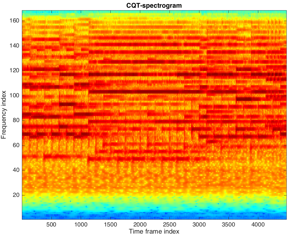
Natural acoustic signals like the musical ones exhibit a highly varying temporal structure, therefore there is a need in adaptive unsupervised methods for signal processing which reduce the complexity of the signal. In [14] a method was proposed which reduces the spectral complexity of music signals using the adaptive segmentation of the signal in the spectral domain for the principal component analysis for listeners with cochlear hearing loss. In the following we apply CPAST and SCPAST as an alternative method for the complexity reduction of music signals. To illustrate the use of SCPAST and CPAST we set the memory parameter γ=0.9\gamma=0.9 to be able to adapt to the changes in the spectral domain of the signal. We focus on the first leading eigenvector recovery. As an example we consider a piece from Bach Siciliano for Oboe and Piano. A wavelet-kind CQT-transform [15] is computed for the signal (see a spectrogram of the transform in Fig. 4). The warmer colors correspond to the higher values of the amplitudes of the harmonics present in the signal at a particular time frame. It is clear that the signal has some regions of “stationarity” (e.g. approximately in time frame interval [1200,2600][1200,2600]). We regard the corresponding spectrogram as a matrix with 45004500 observations of 168168-dimensional signal modeled by (16) and apply SCPAST and CPAST methods to recover the leading eigenvector v1v_{1}.

Refer to caption
Figure 4: CQT-Spectrogram of Bach Siciliano for Oboe and Piano. The deep blue color corresponds to the zero values, the red color corresponds to the higher values.
Refer to caption
Refer to caption
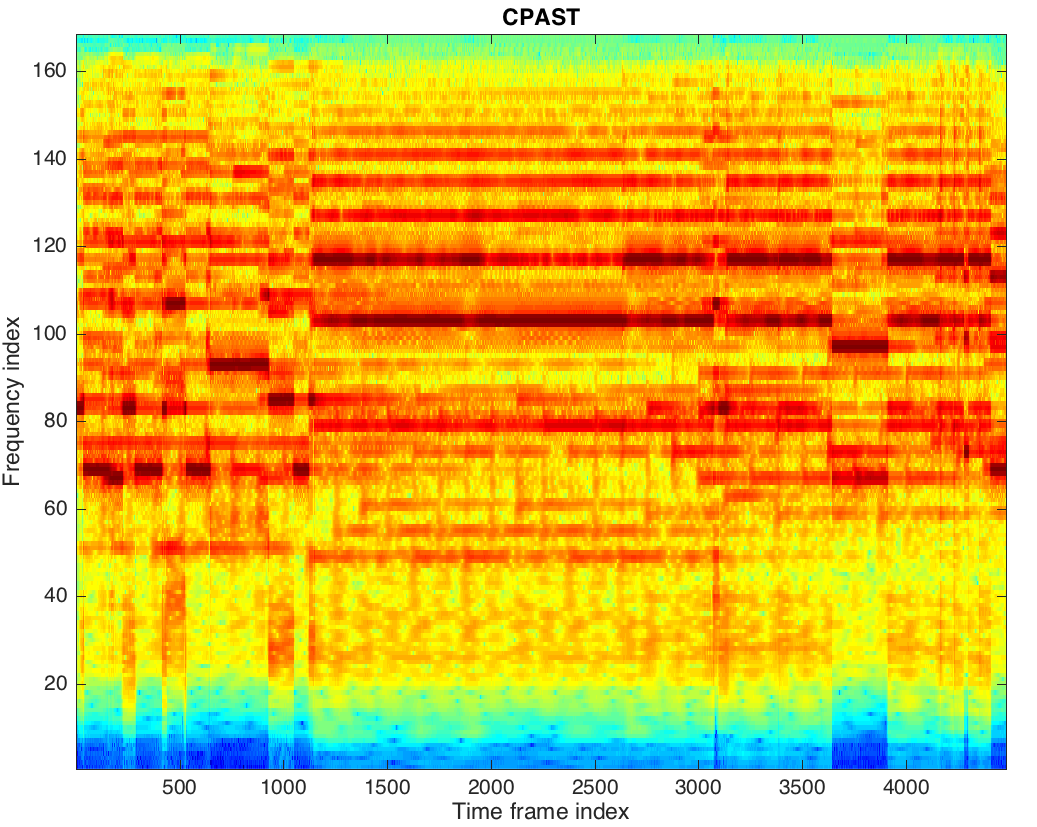
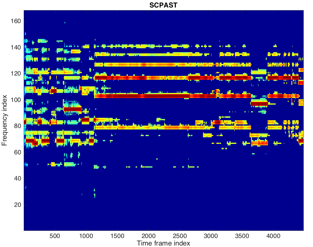
Figure 5: CQT-Spectrogram of the leading eigenvector recovered by CPAST and SCPAST with the memory parameter γ=0.9\gamma=0.9 for Bach Siciliano for Oboe and Piano.

Fig. 5 contains the results of the recovery of the leading eigenvalue with 168168 components. The results show that SCPAST method allows to obtain sparse representation of the leading eigenvectors and seems to be promising for construction of the structure-preserving compressed representations of the signals.

6 Sketch of the proofs

Denote by V¯\bar{V} a matrix with n−dn-d column vectors viv_{i}, i=d+1,…,n,i=d+1,\dots,n, which complete the orthonormal columns {vi}i=1d\{v_{i}\}_{i=1}^{d} of the matrix VV to the orthonormal basis in ℝn\mathbb{R}^{n}. Denote by X⁡(t)X(t) a matrix with the columns {x⁡(i)}i=1t\{x(i)\}_{i=1}^{t}. From (6) one gets a representation

X(t)=VΛd1/2U⊤(t)+σΞ(t),t=1,…,T,X(t)=V\Lambda_{d}^{1/2}U^{\top}(t)+\sigma\Xi(t),\quad t=1,\dots,T, (16)

where U⁡(t)∈ℝt×dU(t)\in\mathbb{R}^{t\times d}, Ξ⁡(t)∈ℝn×t\Xi(t)\in\mathbb{R}^{n\times t} are matrices with independent 𝒩⁡(0,1)\mathcal{N}(0,1) entries, VV is the orthonormal matrix with columns {vi}i=1n\{v_{i}\}_{i=1}^{n}, Λd\Lambda_{d} is a diagonal matrix with λi\lambda_{i}, i=1,…,di=1,\dots,d on the diagonal. Denote a set of indices to the small components of leading eigenvectors as N⁡(t)={1,…,n}\S⁡(t)N(t)=\{1,\dots,n\}\backslash S(t) (where NN here stands for “noise”).

From (16) the empirical covariance matrix can be decomposed as

Σ^​(t)=1t​V​Λd1/2​U⊤​(t)​U​(t)​Λd1/2​V⊤+1t​Ξ​(t)​Ξ⊤​(t)+1t​V​Λd1/2​U⊤​(t)​Ξ⊤​(t)+1t​Ξ​(t)​U​(t)​Λd1/2​V⊤.\begin{split}\widehat{\Sigma}(t)=&\frac{1}{t}V\Lambda^{1/2}_{d}U^{\top}(t)U(t)\Lambda^{1/2}_{d}V^{\top}+\frac{1}{t}\Xi(t)\Xi^{\top}(t)\\ &+\frac{1}{t}V\Lambda^{1/2}_{d}U^{\top}(t)\Xi^{\top}(t)+\frac{1}{t}\Xi(t)U(t)\Lambda^{1/2}_{d}V^{\top}.\end{split} (17)

It is well known [7] that the distance (8) between subspaces 𝒲\mathcal{W} and 𝒬\mathcal{Q}, spanning n×dn\times d matrices with orthonormal columns WW and QQ correspondingly, is related to dd-th principal angle between subspaces 𝒲\mathcal{W} and 𝒬\mathcal{Q} as l⁡(𝒲,𝒬)=sin2⁡ϕd​(𝒲,𝒬),l(\mathcal{W},\mathcal{Q})=\sin^{2}\phi_{d}(\mathcal{W},\mathcal{Q}), where the principal angles 0≤ϕ1≤⋯≤ϕd0\leq\phi_{1}\leq\dots\leq\phi_{d} between subspaces 𝒲\mathcal{W} and 𝒬\mathcal{Q} are recursively defined as [16]

ϕi​(𝒲,𝒬)=arccos⁡⟨xi,yi⟩‖xi‖2​‖yi‖2,where{xi,yi}=arg​minx∈𝒲,y∈𝒬,x⟂xj,y⟂yj,j<i⁡{arccos⁡⟨x,y⟩‖x‖2​‖y‖2}.\begin{split}\phi_{i}(\mathcal{W},\mathcal{Q})&=\arccos\frac{\langle x_{i},y_{i}\rangle}{\|x_{i}\|_{2}\|y_{i}\|_{2}},\,\text{where}\\ \{x_{i},y_{i}\}&=\argmin\limits_{\begin{subarray}{c}x\in\mathcal{W},\,y\in\mathcal{Q},\\ x\perp x_{j},\,y\perp y_{j},\,j<i\end{subarray}}\biggl\{\arccos\frac{\langle x,y\rangle}{\|x\|_{2}\|y\|_{2}}\biggr\}.\end{split}

From the variational characterization of the singular values and the above definition of the principal angles, the dd-th principal angle between subspaces spanning the columns of WW and QQ has the following non-recursive definition

cos⁡ϕd​(W,Q)=\displaystyle\cos\phi_{d}({W},{Q})= =min‖x‖2=1,x∈ℝd⁡‖W⊤​Q​x‖‖Q​x‖,\displaystyle=\min_{\|x\|_{2}=1,\,x\in\mathbb{R}^{d}}\frac{\|W^{\top}Qx\|}{\|Qx\|}, (18)
tan⁡ϕd​(W,Q)=\displaystyle\tan\phi_{d}({W},{Q})= max‖x‖2=1,x∈ℝd⁡‖W¯⊤​Q​x‖‖W⊤​Q​x‖.\displaystyle\max_{\|x\|_{2}=1,\,x\in\mathbb{R}^{d}}\frac{\|\bar{W}^{\top}Qx\|}{\|W^{\top}Qx\|}. (19)

In the next sections we derive the error bounds for CPAST and SCPAST by looking at the change of the dd-th principal angle between the eigensubspace spanning the columns of VV and its estimators based on tt observation, where t=t0+1,…,Tt=t_{0}+1,\dots,T.

6.1 Bound for CPAST

The aim of this section is to show that with the high probability the subspace which spans CPAST estimator V^​(t)\widehat{V}(t) (6.1) is close to the subspace, which spans VV when the number of observations is large enough. We assume that the initial estimator V^0\widehat{V}^{0} is constructed from first t0t_{0} observations with the help of SVD of Σ^​(t0)\widehat{\Sigma}(t_{0}). Let us first state the bound for the error l​(V^​(t),V)l(\widehat{V}(t),V) which depends on the error on the previous iteration l​(V^​(t−1),V)l(\widehat{V}(t-1),V) for the fixed t=t0+1,…,Tt=t_{0}+1,\dots,T. Denote r⁡(t)=l1/2​(V^​(t),V)=sin⁡ϕd​(V^​(u),V)r(t)=l^{1/2}(\widehat{V}(t),V)=\sin\phi_{d}(\widehat{V}(u),V).

Lemma 1.

For CPAST (4) with probability 1−C0​(n∨t)−31-C_{0}(n\vee t)^{-3}

r⁡(t)≤(λd+1+1)tanϕd(V^(t−1),V)λd+1−(λ1+1)E(t)secϕd(V^(t−1),V)+(λ1+1)1/2E(t)secϕd(V^(t−1),V)λd+1−(λ1+1)E(t)secϕd(V^(t−1),V),\begin{split}r(t)\leq&\frac{(\lambda_{d+1}+1)\tan\phi_{d}(\widehat{V}(t-1),V)}{\lambda_{d}+1-(\lambda_{1}+1)E(t)\sec\phi_{d}(\widehat{V}(t-1),V)}\\ &+\frac{(\lambda_{1}+1)^{1/2}E(t)\sec\phi_{d}(\widehat{V}(t-1),V)}{\lambda_{d}+1-(\lambda_{1}+1)E(t)\sec\phi_{d}(\widehat{V}(t-1),V)},\end{split} (20)

where

E⁡(t)=5​n−dt+5​6​log⁡(n∨t)t.E(t)=5\sqrt{\frac{n-d}{t}}+5\sqrt{6}\sqrt{\frac{\log(n\vee t)}{t}}.

The following lemma gives the bound for the error l​(V^​(u),V)l(\widehat{V}(u),V) depending on the error of the previous iteration l​(V^​(u−1),V)l(\widehat{V}(u-1),V) for all u∈{t0+1,…,t}u\in\{t_{0}+1,\dots,t\}.

Lemma 2.

With probability greater than

1−C0​(n∨t)−31-C_{0}(n\vee t)^{-3}

for all u∈{t0+1,…,t}u\in\{t_{0}+1,\dots,t\}

r⁡(u)≤α0​r​(u−1)+α1​R⁡(t)u1−r2​(u−1)−α2​R⁡(t)u,r(u)\leq\frac{\alpha_{0}r(u-1)+\alpha_{1}\frac{R(t)}{\sqrt{u}}}{\sqrt{1-r^{2}(u-1)}-\alpha_{2}\frac{R(t)}{\sqrt{u}}}, (21)

where r⁡(u)=sin⁡ϕd​(V^​(u),V)r(u)=\sin\phi_{d}(\widehat{V}(u),V),

R⁡(t)=5​n−d+5​6​log⁡(n∨t),R(t)=5\sqrt{n-d}+5\sqrt{6}\sqrt{\log(n\vee t)},
α0=1λd+1,α1=λ1+1λd+1,α2=λ1+1λd+1.\begin{split}\alpha_{0}=\frac{1}{\lambda_{d}+1},\quad\alpha_{1}=\frac{\sqrt{\lambda_{1}+1}}{{\lambda_{d}+1}},\quad\alpha_{2}=\frac{\lambda_{1}+1}{\lambda_{d}+1}.\end{split} (22)

Given Lemma 2 it is possible to derive a bound for l​(V^​(t),V)l(\widehat{V}(t),V). First let us state the result which allows to bound the error of the initial estimate V^​(t0)\widehat{V}(t_{0}).

Lemma 3.

Let V^​(t0)\widehat{V}(t_{0}) be a matrix containing first dd leading eigenvectors of the matrix Σ^​(t0)\widehat{\Sigma}(t_{0}). Then with probability 1−C0​(n∨T)−21-C_{0}(n\vee T)^{-2}

r2​(t0)=l⁡(V^​(t0),V)≤α2​1t0,r^{2}(t_{0})=l(\widehat{V}(t_{0}),V)\leq\alpha^{2}\frac{1}{t_{0}},

where α=Rmax​λ1+1λd,\alpha=R_{\max}\frac{\lambda_{1}+1}{\lambda_{d}}, with Rmax=R⁡(T)R_{\max}=R(T).

The following Lemma gives the error of CPAST after observing KK vectors xix_{i}, i=t0+1,…,t0+Ki=t_{0}+1,\dots,t_{0}+K based on the recursive bound (21). Note that the proof of Lemma 4 also insures that the denominator in (21) is bounded away from zero.

Lemma 4.

Suppose that r⁡(t0)≤α​1t0r(t_{0})\leq\alpha\frac{1}{\sqrt{t_{0}}}, where

t0≥8​Rmax​α2(1−α0)3/2.\sqrt{t_{0}}\geq 8R_{\max}\frac{\alpha_{2}}{(1-\alpha_{0})^{3/2}}.

Then for K≥K⁡(ρ,t0)K\geq K(\rho,t_{0})

r⁡(t0+K)≤2​α1α0​11−α0​R⁡(t0+K)K+t0.r(t_{0}+K)\leq 2\frac{\alpha_{1}}{\alpha_{0}}\frac{1}{1-\alpha_{0}}\frac{R(t_{0}+K)}{\sqrt{K+t_{0}}}. (23)

The statement of the Theorem 1 follows from Lemma 2 applied to the inequality (21) with (22), which holds with probability 1−C0​(n∨t)−21-C_{0}(n\vee t)^{-2} with the initial conditions given by Lemma 3.

6.2 Bound for SCPAST

Define Σ^∘​(t)\widehat{\Sigma}^{\circ}(t), the oracle version of Σ^​(t)\widehat{\Sigma}(t) and the corresponding expectation Σ∘​(t)=𝐄​Σ^∘​(t){\Sigma}^{\circ}(t)=\mathbf{E}\widehat{\Sigma}^{\circ}(t) as follows

Σ^∘​(t)=[Σ^S​(t)00IN⁡(t)],Σ∘​(t)=[ΣS​(t)00IN⁡(t)],\widehat{\Sigma}^{\circ}(t)=\left[\begin{matrix}\widehat{\Sigma}_{S}(t)&0\\ 0&I_{N(t)}\end{matrix}\right],\,{\Sigma}^{\circ}(t)=\left[\begin{matrix}\Sigma_{S}(t)&0\\ 0&I_{N(t)}\end{matrix}\right], (24)

where Σ^S⁡(t)\widehat{\Sigma}_{S(t)} and ΣS​(t)\Sigma_{S}(t) are the sub-matrices of the size card⁡(S⁡(t))×card⁡(S⁡(t)){\rm card}(S(t))\times{\rm card}(S(t)) with column and row indices from S⁡(t)S(t). The identity matrix IN⁡(t)I_{N(t)} has the size card⁡(N⁡(t))×card⁡(N⁡(t)){\rm card}{(N(t))}\times{\rm card}{(N(t))}. Here we assumed without loss of generality that indices in S⁡(t){S(t)} are always smaller than ones in N⁡(t)N(t).

First we obtain the oracle sequence V^∘​(t)\widehat{V}^{\circ}(t) of the solutions by iterating SCPAST with matrices Σ^∘​(t)\widehat{\Sigma}^{\circ}(t) instead of Σ^​(t)\widehat{\Sigma}(t). We define the initial estimate V^∘​(t0)\widehat{V}^{\circ}(t_{0}) with the steps (a)-(d) in the section 6.1 applied to the matrix Σ^∘​(t0)\widehat{\Sigma}^{\circ}(t_{0}). And then bound sin⁡ϕd​(V^∘​(t),V)\sin\phi_{d}(\widehat{V}^{\circ}(t),V). Denote the result of the thresholding the columns of the matrix Υ^∘​(t)=Σ^∘​(t)​V^​(t−1)\widehat{\Upsilon}^{\circ}(t)=\widehat{\Sigma}^{\circ}(t)\widehat{V}(t-1) with the thresholding parameters given by the vector β⁡(t)\beta(t) as

Υ^∘,β​(t)=g⁡(Υ^∘​(t),β⁡(t)).\widehat{\Upsilon}^{\circ,\beta}(t)=g(\widehat{\Upsilon}^{\circ}(t),\beta(t)).

Denote the submatrix VS​(t)V_{S}(t) obtained by selecting the rows of VV with indices in S⁡(t)S(t). Denote by VkV_{k}, k=1,…,nk=1,\dots,n the rows of VV (recall that the columns are vjv_{j}, j=1,…,mj=1,\dots,m). For the estimators of VV we omit the dependence of S⁡(t)S(t) on tt as the estimator itself depends on tt, that is, V^S​(t)\widehat{V}_{S}(t) is a matrix of the rows of V^​(t)\widehat{V}(t) with indices from S⁡(t)S(t).

The following bound for the oracle error r2​(t)=l⁡(V^∘​(t),V)r^{2}(t)=l(\widehat{V}^{\circ}(t),V) of SCPAST method is analogous to Lemma 2.

Lemma 5.

For u=t0+1,…,tu=t_{0}+1,\dots,t with probability greater than 1−C0​(n∨t)−31-C_{0}(n\vee t)^{-3} the following bound holds true

r⁡(u)≤α0​r​(u−1)+α1​R∘​(t)u1−r2​(u−1)−α2​R∘​(t)u,where r(u)\leq\frac{\alpha_{0}r(u-1)+\alpha_{1}\frac{R^{\circ}(t)}{\sqrt{u}}}{\sqrt{1-r^{2}(u-1)}-\alpha_{2}\frac{R^{\circ}(t)}{\sqrt{u}}},\quad\text{where } (25)
α0=(λd+1)−1,α1=α2=(λ1+1)/(λd+1),\begin{split}\alpha_{0}&=(\lambda_{d}+1)^{-1},\quad\alpha_{1}=\alpha_{2}=(\lambda_{1}+1)/\penalty(\lambda_{d}+1),\end{split} (26)

R∘​(t)=C1​hd​M1/2​(t)​log⁡(n∨t)+C2​log⁡(n∨t)R^{\circ}(t)=C_{1}h_{d}M^{1/2}(t)\sqrt{\log(n\vee t)}+C_{2}\sqrt{\log(n\vee t)}, where C0C_{0} and C2C_{2} are constants and C1C_{1} depends on rr, dd, aa, τ\tau.

In the sparse case the similar result to Lemma 3 holds true giving a bound on the error of the initial oracle estimator.

Lemma 6.

The error of initial oracle estimation is bounded as follows r⁡(t0)≤αt0,r(t_{0})\leq\frac{\alpha}{\sqrt{t_{0}}}, with probability 1−C0​(n∨T)−21-C_{0}(n\vee T)^{-2}, where

α=(1λd​C1​λ1​hd​M1/2​(t0)+C2​λ1+1λd)​log⁡(n∨T),\alpha=\left(\frac{1}{\lambda_{d}}C_{1}\lambda_{1}h_{d}M^{1/2}(t_{0})+C_{2}\frac{\lambda_{1}+1}{\lambda_{d}}\right)\sqrt{{\log(n\vee T)}},

where C0C_{0} and C2C_{2} are constants and C1C_{1} depends on rr.

Lemma 7.

Thus after tt iterations, t=t0+1,…,Tt=t_{0}+1,\dots,T, with the probability 1−C0​(n∨t)−21-C_{0}(n\vee t)^{-2} one has

l⁡(V,V^∘​(t))≤C1​hd2​M​(t)​log⁡(n∨t)t+C2​λ1+1λd2​log⁡(n∨t)t,\begin{split}l(V,\widehat{V}^{\circ}(t))\leq&C_{1}h_{d}^{2}M(t)\frac{\log(n\vee t)}{t}+C_{2}\frac{\lambda_{1}+1}{\lambda_{d}^{2}}\frac{\log(n\vee t)}{t},\end{split}

where C1C_{1} depends on dd, rr, τ\tau, aa, and C2C_{2} depends on τ\tau.

The convergence of the oracle scheme doesn’t immediately imply the convergence of the SCPAST estimators. The following two lemmas state that with the high probability V^∘​(t)=V^​(t)\widehat{V}^{\circ}(t)=\widehat{V}(t). Thus the bound in Lemma 7 holds for SCPAST and the Theorem 2 is justified.

Lemma 8.

For γ0≥3​2​log⁡(n∨T)log⁡(n∨t0)\gamma_{0}\geq 3\sqrt{2}\frac{\log(n\vee T)}{\log(n\vee t_{0})} with probability 1−C0​(n∨T)−21-C_{0}(n\vee T)^{-2} the initial oracle estimate coincide with the initial SPCA estimate, that is, V^∘​(t0)=V^​(t0)\widehat{V}^{\circ}(t_{0})=\widehat{V}(t_{0}).

Lemma 9.

With probability 1−C0​(n∨t)−21-C_{0}(n\vee t)^{-2} for u=t0+1,…,tu=t_{0}+1,\dots,t the oracle SCPAST and SCPAST solutions coincide V^∘​(t)=V^​(t)\widehat{V}^{\circ}(t)=\widehat{V}(t).

Conclusions

We developed a new method SCPAST based on constraint projection approximation subspace tracking method for subspace tracking in the sparsity assumptions on the underlying signal eigen subspace. The thesholding step was introduced in order to ensure the sparsity of the solution. We presented the non-asymptotical bounds for the errors of subspace recovery with SCPAST and CPAST as well as the empirical studies of the methods. The results of experiments show that SCPAST method allows to obtain sparse representation of the leading eigenvector of music signals and might be used for adaptive compression of the musical signal in the spectral domain.

Appendix A. Proofs of Lemmas

Proof of Lemma 1

From the definition (19) tan⁡ϕd​(Σ^​(t)​V^​(t−1),V)=max‖x‖2=1⁡‖V¯⊤​Σ^​(t)​V^​(t−1)​x‖‖V⊤​Σ^​(t)​V^​(t−1)​x‖\tan\phi_{d}(\widehat{\Sigma}(t)\widehat{V}(t-1),V)=\max_{\|x\|_{2}=1}\frac{\|\bar{{V}}^{\top}\widehat{\Sigma}(t)\widehat{V}(t-1)x\|}{\|V^{\top}\widehat{\Sigma}(t)\widehat{V}(t-1)x\|}. Using Σ^​(t)=Σ^​(t)−Σ+Σ\widehat{\Sigma}(t)=\widehat{\Sigma}(t)-\Sigma+\Sigma the latter maximum can be bounded by

max‖x‖2=1⁡‖V¯⊤​V^​(t−1)​x‖+‖V¯⊤​(Σ^​(t)−Σ)​V^​(t−1)​x‖(λd+1)​‖V⊤​V^​(t−1)​x‖−‖V⊤​(Σ^​(t)−Σ)​V^​(t−1)​x‖.\displaystyle\max_{\|x\|_{2}=1}\frac{\|\bar{{V}}^{\top}\widehat{V}(t-1)x\|+\|\bar{{V}}^{\top}(\widehat{\Sigma}(t)-\Sigma)\widehat{V}(t-1)x\|}{(\lambda_{d}+1)\|V^{\top}\widehat{V}(t-1)x\|-\|V^{\top}(\widehat{\Sigma}(t)-\Sigma)\widehat{V}(t-1)x\|}.

Using (18)

max‖x‖2=1\displaystyle\max_{\|x\|_{2}=1} ‖V¯⊤​(Σ^​(t)−Σ)​V^​(t−1)​x‖‖V⊤​V^​(t−1)​x‖≤‖V¯⊤​(Σ^​(t)−Σ)‖cos⁡ϕd​(V^​(t−1),V),\displaystyle\frac{\|\bar{V}^{\top}(\widehat{\Sigma}(t)-\Sigma)\widehat{V}(t-1)x\|}{\|V^{\top}\widehat{V}(t-1)x\|}\leq\frac{\|\bar{V}^{\top}(\widehat{\Sigma}(t)-\Sigma)\|}{\cos\phi_{d}(\widehat{V}(t-1),V)},
max‖x‖2=1\displaystyle\max_{\|x\|_{2}=1} ‖V⊤​(Σ^​(t)−Σ)​V^​(t−1)​x‖‖V⊤​V^​(t−1)​x‖≤‖V⊤​(Σ^​(t)−Σ)‖cos⁡ϕd​(V^​(t−1),V).\displaystyle\frac{\|V^{\top}(\widehat{\Sigma}(t)-\Sigma)\widehat{V}(t-1)x\|}{\|V^{\top}\widehat{V}(t-1)x\|}\leq\frac{\|V^{\top}(\widehat{\Sigma}(t)-\Sigma)\|}{\cos\phi_{d}(\widehat{V}(t-1),V)}.

From (17)

Σ^​(t)=Σ+1t​Ξ​(t)​Ξ⊤​(t)−In+1t​V​Λd1/2​U⊤​(t)​Ξ⊤​(t)+1t​Ξ​(t)​U​(t)​Λd1/2​V⊤+V​Λd1/2​(1t​U⊤​(t)​U​(t)−Id)​Λd1/2​V⊤.\begin{split}\widehat{\Sigma}(t)=&\Sigma+\frac{1}{t}\Xi(t)\Xi^{\top}(t)-I_{n}\\ &+\frac{1}{t}V\Lambda^{1/2}_{d}U^{\top}(t)\Xi^{\top}(t)+\frac{1}{t}\Xi(t)U(t)\Lambda^{1/2}_{d}V^{\top}\\ &+V\Lambda^{1/2}_{d}\left(\frac{1}{t}U^{\top}(t)U(t)-I_{d}\right)\Lambda^{1/2}_{d}V^{\top}.\end{split} (27)

Therefore using V¯​V¯⊤+V​V⊤=In\bar{V}\bar{V}^{\top}+VV^{\top}=I_{n}

‖V¯⊤​(Σ^​(t)−Σ)‖≤\displaystyle\|\bar{V}^{\top}(\widehat{\Sigma}(t)-\Sigma)\|\leq ‖1t​V¯⊤​Ξ​(t)​[V¯⊤​Ξ​(t)]⊤−In−d‖\displaystyle\left\|\frac{1}{t}\bar{V}^{\top}\Xi(t)[\bar{V}^{\top}\Xi(t)]^{\top}-I_{n-d}\right\|
+1t​‖V¯⊤​Ξ​(t)​[V⊤​Ξ​(t)]⊤‖\displaystyle+\frac{1}{t}\|\bar{V}^{\top}\Xi(t)[{V}^{\top}\Xi(t)]^{\top}\|
+λ1​1t​‖V¯⊤​Ξ​(t)​U​(t)‖,\displaystyle+\sqrt{\lambda_{1}}\frac{1}{t}\|\bar{V}^{\top}\Xi(t)U(t)\|,
‖V⊤​(Σ^​(t)−Σ)‖≤\displaystyle\|{V}^{\top}(\widehat{\Sigma}(t)-\Sigma)\|\leq λ1​‖1t​U⊤​(t)​U​(t)−Id‖\displaystyle\lambda_{1}\left\|\frac{1}{t}U^{\top}(t)U(t)-I_{d}\right\|
+‖1t​V⊤​Ξ​(t)​[V¯⊤​Ξ​(t)]⊤‖\displaystyle+\left\|\frac{1}{t}{V}^{\top}\Xi(t)[{\bar{V}}^{\top}\Xi(t)]^{\top}\right\|
+‖1t​V⊤​Ξ​(t)​[V⊤​Ξ​(t)]⊤−Id‖\displaystyle+\left\|\frac{1}{t}{V}^{\top}\Xi(t)\left[{V}^{\top}\Xi(t)\right]^{\top}-I_{d}\right\|
+2​λ1​‖1t​Ξ​(t)​U​(t)‖.\displaystyle+2{\sqrt{\lambda_{1}}}\left\|\frac{1}{t}\Xi(t)U(t)\right\|.

Using λ1∨1≤λ1+1≤λ1+1\sqrt{\lambda_{1}}\vee 1\leq\sqrt{\lambda_{1}+1}\leq\lambda_{1}+1, Lemma 10 and Lemma 11 with p=6p=\sqrt{6} we bound the terms to the right of the above two inequalities with the probability 1−C0​(n∨t)−31-C_{0}(n\vee t)^{-3}, for big enough tt

‖V¯⊤​(Σ^​(t)−Σ)‖≤λ1+1​E​(t),‖V⊤​(Σ^​(t)−Σ)‖≤(λ1+1)​E​(t),\begin{split}\|\bar{V}^{\top}(\widehat{\Sigma}(t)-\Sigma)\|&\leq\sqrt{\lambda_{1}+1}E(t),\\ \|V^{\top}(\widehat{\Sigma}(t)-\Sigma)\|&\leq(\lambda_{1}+1)E(t),\end{split} (28)

where E⁡(t)=5​n−dt+5​6​log⁡(n∨t)tE(t)=5\sqrt{\frac{n-d}{t}}+5\sqrt{6}\sqrt{\frac{\log(n\vee t)}{t}} with probability 1−C0​(n∨t)−31-C_{0}(n\vee t)^{-3}, where C0C_{0} is a constant. The statement of the lemma follows from the observation that

tan⁡ϕd​(V^​(t),V)=tan⁡ϕd​(Σ^​(t)​V^​(t−1),V).\tan\phi_{d}(\widehat{V}(t),V)=\tan\phi_{d}(\widehat{\Sigma}(t)\widehat{V}(t-1),V).

Proof of Lemma 2

Lemma 1 gives a probabilistic bound on the error of subspace estimation l​(V^​(t),V)l(\widehat{V}(t),V) based on the previous iteration l​(V^​(t−1),V)l(\widehat{V}(t-1),V). Or goal is to bound l​(V^​(t),V)l(\widehat{V}(t),V) for t∈{t0+1,…,T}t\in\left\{t_{0}+1,\dots,T\right\}. Due to Lemmas (10) and (11) we get for p>1p>1, u=t0+1,…,tu=t_{0}+1,\dots,t the term u​‖1u​V⊤​Ξ​(u)​[V⊤​Ξ​(u)]⊤−Id‖\sqrt{u}\left\|\frac{1}{u}{V}^{\top}\Xi(u)\left[{V}^{\top}\Xi(u)\right]^{\top}-I_{d}\right\| is bounded from above by 3​(d+p​log⁡(n∨t))3(\sqrt{d}+p\sqrt{\log(n\vee t)}), u​‖1u​V¯⊤​Ξ​(u)​[V¯⊤​Ξ​(u)]⊤−In−d‖\sqrt{u}\left\|\frac{1}{u}\bar{V}^{\top}\Xi(u)[\bar{V}^{\top}\Xi(u)]^{\top}-I_{n-d}\right\| by 3​(n−d+p​log⁡(n∨t))3(\sqrt{n-d}+p\sqrt{\log(n\vee t)}), u​‖1u​V⊤​Ξ​(u)​[V¯⊤​Ξ​(u)]⊤‖\sqrt{u}\left\|\frac{1}{u}{V}^{\top}\Xi(u)[{\bar{V}}^{\top}\Xi(u)]^{\top}\right\| by 1+2​p​log⁡(n∨t)u​(n−d+d+p​log⁡(n∨t))\sqrt{1+2p\frac{\log(n\vee t)}{\sqrt{u}}}(\sqrt{n-d}+\sqrt{d}+p\sqrt{\log(n\vee t)}). Finally, u​‖1u​V¯⊤​Ξ​(u)​U​(u)‖\sqrt{u}\left\|\frac{1}{u}\bar{V}^{\top}\Xi(u)U(u)\right\| is bounded by

1+2​p​log⁡(n∨t)u​(n−d+d+p​log⁡(n∨t)).\sqrt{1+2p\frac{\log(n\vee t)}{\sqrt{u}}}(\sqrt{n-d}+\sqrt{d}+p\sqrt{\log(n\vee t)}).

Each of the bounds holds with the probability 1−(n∨t)−31-(n\vee t)^{-3} for p=6p=\sqrt{6}. Using the union bound we get the statement of the Lemma for the intersection of events with the probability 1−C0​(t−t0)​(n∨t)−31-C_{0}(t-t_{0})(n\vee t)^{-3}.

Proof of Lemma 3

The proof is based on Davis sin⁡θ\sin\theta Theorem 4, Lemma 10 (see Appendix B), and Weyl’s theorem [17]. From Davis sin⁡θ\sin\theta Theorem

l⁡(V,V^​(t0))≤‖(Σ^​(t0)−Σ)​V‖2(λd+1−λd+1​(Σ^​(t0)))2,\begin{split}l(V,\widehat{V}(t_{0}))\leq\frac{\left\|(\widehat{\Sigma}(t_{0})-\Sigma)V\right\|^{2}}{\left(\lambda_{d}+1-\lambda_{d+1}\left(\widehat{\Sigma}(t_{0})\right)\right)^{2}},\end{split} (29)

where λd+1​(A)\lambda_{d+1}(A) is a (d+1)(d+1)-th singular value of the matrix AT​AA^{T}A. Weil’s theorem gives for j=1,…,nj=1,\dots,n

|λj+1−λj​(Σ^​(t0))|≤‖Σ^​(t0)−Σ‖.|\lambda_{j}+1-\lambda_{j}(\widehat{\Sigma}(t_{0}))|\leq\|\widehat{\Sigma}(t_{0})-\Sigma\|.

Therefore the denominator in (29) may be bounded as

|λd+1−λd+1​(Σ^​(t0))|≥λd−2​‖Σ^​(t0)−Σ‖.|\lambda_{d}+1-\lambda_{d+1}(\widehat{\Sigma}(t_{0}))|\geq\lambda_{d}-2\|\widehat{\Sigma}(t_{0})-\Sigma\|.

From (27)

‖Σ^​(t0)−Σ‖≤\displaystyle\|\widehat{\Sigma}(t_{0})-\Sigma\|\leq λ1​‖1t0​U​(t0)⊤​U​(t0)−Id‖\displaystyle\lambda_{1}\left\|\frac{1}{t_{0}}U(t_{0})^{\top}U(t_{0})-I_{d}\right\|
+‖1t​Ξ​(t0)​Ξ⊤​(t0)−In‖\displaystyle+\left\|\frac{1}{t}\Xi(t_{0})\Xi^{\top}(t_{0})-I_{n}\right\|
+2​λ1​‖1t0​U⊤​(t0)​Ξ⊤​(t0)‖,\displaystyle+2\sqrt{\lambda_{1}}\left\|\frac{1}{t_{0}}U^{\top}(t_{0})\Xi^{\top}(t_{0})\right\|,

by Lemma 10 and 11

|λd+1−λd+1​(Σ^​(t0))|≥(1+o⁡(1))​λd.|\lambda_{d}+1-\lambda_{d+1}(\widehat{\Sigma}(t_{0}))|\geq(1+o(1))\lambda_{d}.

From (28) and Lemma 10 one has that with probability 1−C0​(n∨t)−21-C_{0}(n\vee t)^{-2}

‖(Σ^​(t0)−Σ)​V‖≤(λ1+1)​(nt0+log⁡(n∨t)t0).\|(\widehat{\Sigma}(t_{0})-\Sigma)V\|\leq(\lambda_{1}+1)\left(\sqrt{\frac{n}{t_{0}}}+\sqrt{\frac{\log(n\vee t)}{t_{0}}}\right).

Combining the last two inequalities we get the statement of Lemma.

Proof of Lemma 4

First we prove (23) for the pair (t0,r⁡(t0))(t_{0},r(t_{0})) which satisfies by induction for all k=1,…,K,k=1,\ldots,K, and some ρ∈(α0,1)\rho\in(\alpha_{0},1)

1−(r⁡(t0)+R⁡(α1α0)​ρ1−ρ​1t0)2−α2​Rt0>α0ρ.\sqrt{1-\left(r(t_{0})+R\left(\frac{\alpha_{1}}{\alpha_{0}}\right)\frac{\rho}{1-\rho}\frac{1}{\sqrt{t_{0}}}\right)^{2}}-\frac{\alpha_{2}R}{\sqrt{t_{0}}}>\frac{\alpha_{0}}{\rho}. (30)

We have for K=1K=1

r⁡(t0+1)≤α0​r​(t0)+α1​Rt0+11−r2​(t0)−α2​Rt0+1≤ρ​r​(t0)+ρ​α1α0​Rt0+1.r(t_{0}+1)\leq\frac{\alpha_{0}r(t_{0})+\alpha_{1}\frac{R}{\sqrt{t_{0}+1}}}{\sqrt{1-r^{2}(t_{0})}-\alpha_{2}\frac{R}{\sqrt{t_{0}+1}}}\leq\rho r(t_{0})+\frac{\rho\alpha_{1}}{\alpha_{0}}\frac{R}{\sqrt{t_{0}+1}}.

Furthermore suppose that (30) holds for K=L,K=L, then

r2​(t+L)≤(ρL​r​(t0)+R⁡(α1α0)​∑k=1LρL+1−kt0+k)2r^{2}(t+L)\leq\left(\rho^{L}r(t_{0})+R\left(\frac{\alpha_{1}}{\alpha_{0}}\right)\sum_{k=1}^{L}\frac{\rho^{L+1-k}}{\sqrt{t_{0}+k}}\right)^{2}

and

r⁡(t0+L+1)\displaystyle r(t_{0}+L+1) ≤α0​r​(t+L)+α1​Rt+L+11−r2​(t+L)−α2​Rt+L+1\displaystyle\leq\frac{\alpha_{0}r(t+L)+\alpha_{1}\frac{R}{\sqrt{t+L+1}}}{\sqrt{1-r^{2}(t+L)}-\alpha_{2}\frac{R}{\sqrt{t+L+1}}}
≤ρL​r​(t0)+R⁡(α1α0)​∑k=1L+1ρ1+L−kt0+k.\displaystyle\leq\rho^{L}r(t_{0})+R\left(\frac{\alpha_{1}}{\alpha_{0}}\right)\sum_{k=1}^{L+1}\frac{\rho^{1+L-k}}{\sqrt{t_{0}+k}}.

A sufficient condition for the above formula to hold reads as

1−(ρk−1​r​(t0)+α1​Rα0​∑j=1k−1ρk−jt0+j)2−α2​Rt0+k>α0ρ.\sqrt{1-\left(\rho^{k-1}r(t_{0})+\frac{\alpha_{1}R}{\alpha_{0}}\sum_{j=1}^{k-1}\frac{\rho^{k-j}}{\sqrt{t_{0}+j}}\right)^{2}}-\frac{\alpha_{2}R}{\sqrt{t_{0}+k}}>\frac{\alpha_{0}}{\rho}.

Note that ∑j=1k−1ρk−jt0+j≤ρ1−ρ​1t0,\sum_{j=1}^{k-1}\frac{\rho^{k-j}}{\sqrt{t_{0}+j}}\leq\frac{\rho}{1-\rho}\frac{1}{\sqrt{t_{0}}}, therefore the above condition is fulfilled given (30). Furthermore

r⁡(t0+K+1)≤ρK​r​(t0)+R⁡(α1α0)​∑k=1K+1ρ1+K−kt0+k,\displaystyle r(t_{0}+K+1)\leq\rho^{K}r(t_{0})+R\left(\frac{\alpha_{1}}{\alpha_{0}}\right)\sum_{k=1}^{K+1}\frac{\rho^{1+K-k}}{\sqrt{t_{0}+k}},

where for K>K0​(ρ)K>K_{0}(\rho), t0>1t_{0}>1 and jK,ρ=log⁡(K)/(2​log⁡(1/ρ))j_{K,\rho}=\log(K)/(2\log(1/\rho))

∑k=1KρK−kt0+k≤\displaystyle\sum_{k=1}^{K}\frac{\rho^{K-k}}{\sqrt{t_{0}+k}}\leq ∑j=0jK,ρρjt0+K−j+∑j=jK,ρ+1K−1ρjt0+K−j\displaystyle\sum_{j=0}^{j_{K,\rho}}\frac{\rho^{j}}{\sqrt{t_{0}+K-j}}+\sum_{j=j_{K,\rho}+1}^{K-1}\frac{\rho^{j}}{\sqrt{t_{0}+K-j}}
≤11−ρ​1t0+K−jK,ρ+11−ρ​1K+t0\displaystyle\leq\frac{1}{1-\rho}\frac{1}{\sqrt{t_{0}+K-j_{K,\rho}}}+\frac{1}{1-\rho}\frac{1}{\sqrt{K+t_{0}}}

and

r⁡(t0+K+1)≲α1α0​ρ1−ρ​RK+t0+1.r(t_{0}+K+1)\lesssim\frac{\alpha_{1}}{\alpha_{0}}\frac{\rho}{1-\rho}\frac{R}{\sqrt{K+t_{0}+1}}.

From (30) the condition on the starting value r⁡(t0)r(t_{0}) is

r⁡(t0)≤1−(α2​Rt0+α0ρ)2−R​α1α0​ρ1−ρ​1t0.r(t_{0})\leq\sqrt{1-\left(\alpha_{2}\frac{R}{\sqrt{t_{0}}}+\frac{\alpha_{0}}{\rho}\right)^{2}}-\frac{R\alpha_{1}}{\alpha_{0}}\frac{\rho}{1-\rho}\frac{1}{\sqrt{t_{0}}}. (31)

Thus the number of initial observations t0t_{0} for (31) to be satisfied given r⁡(t0)≤α​1t0r(t_{0})\leq\alpha\frac{1}{\sqrt{t_{0}}} reads as

α​1t0≤1−(α2​Rt0+α0ρ)2−R⁡(α1α0)​11−ρ​1t0.\alpha\frac{1}{\sqrt{t_{0}}}\leq\sqrt{1-\left(\alpha_{2}\frac{R}{\sqrt{t_{0}}}+\frac{\alpha_{0}}{\rho}\right)^{2}}-R\left(\frac{\alpha_{1}}{\alpha_{0}}\right)\frac{1}{1-\rho}\frac{1}{\sqrt{t_{0}}}.

Therefore, taking into account (26) and ρ>α0\rho>\alpha_{0}, the sufficient condition on t0\sqrt{t_{0}} is

t0≥2​α2​R(1−α02ρ2)+2​R​(α1α0)​ρ1−ρ1−α02ρ2.\sqrt{t_{0}}\geq\frac{2\alpha_{2}{R}}{\left(1-\frac{\alpha^{2}_{0}}{\rho^{2}}\right)}+\frac{2R\left(\frac{\alpha_{1}}{\alpha_{0}}\right)\frac{\rho}{1-\rho}}{\sqrt{1-\frac{\alpha^{2}_{0}}{\rho^{2}}}}.

From Lemma 3 and (26) α=Rmax​α21−α0.{\alpha}={R_{\max}}\frac{\alpha_{2}}{1-\alpha_{0}}. Set ρ=ρ⁡(ϵ)=1−ϵ⁡(1−α0)\rho=\rho(\epsilon)=1-\epsilon(1-\alpha_{0}). It is easy to check that α0<ρ⁡(ϵ)<1\alpha_{0}<\rho(\epsilon)<1 for ϵ∈(0,1/2]\epsilon\in(0,1/2]. Recall Rmax=R⁡(T)R_{\max}=R(T), therefore

t0≥2​Rmax​α2ϵ​(1−α0)3/2​11−ϵ.\sqrt{t_{0}}\geq\frac{2R_{\max}\alpha_{2}}{\epsilon(1-\alpha_{0})^{3/2}}\frac{1}{\sqrt{1-\epsilon}}.

The value K0​(ρ)K_{0}(\rho) might be defined by ρK≤α1α0​Rt0+K,\rho^{K}\leq\frac{\alpha_{1}}{\alpha_{0}}\frac{R}{\sqrt{t_{0}+K}}, thus (using |ln⁡(1−x)|≥x|\ln(1-x)|\geq x for x∈(0,1)x\in(0,1)) it is sufficient to set K≥1ϵ⁡(1−α0)​ln⁡(α0α1​T).K\geq\frac{1}{\epsilon(1-\alpha_{0})}\ln\left(\frac{\alpha_{0}}{\alpha_{1}}\sqrt{T}\right). Put ϵ=1/2\epsilon=1/2 to get the result.

Proof of Lemma 5

Using the triangle inequality

l​(V^∘​(t),V)≤l​(Υ^∘​(t),V)+l⁡(Υ^∘​(t),V^∘​(t)).\displaystyle\sqrt{l(\widehat{V}^{\circ}(t),V)}\leq\sqrt{l(\widehat{\Upsilon}^{\circ}(t),V)}+\sqrt{l(\widehat{\Upsilon}^{\circ}(t),\widehat{V}^{\circ}(t))}. (32)

We bound the first term as

l1/2​(Υ^∘​(t),V)≤tan⁡ϕd​(Σ^∘​(t)​V^∘​(t−1),V).l^{1/2}(\widehat{\Upsilon}^{\circ}(t),V)\leq\tan\phi_{d}(\widehat{\Sigma}^{\circ}(t)\widehat{V}^{\circ}(t-1),V).

Using the variational definition of tan⁡ϕd\tan\phi_{d}

l1/2​(Υ^∘​(t),V)≤max‖x‖2=1⁡‖V¯⊤​Σ^∘​(t)​V^∘​(t−1)​x‖‖V⊤​Σ^∘​(t)​V^∘​(t−1)​x‖\begin{split}&l^{1/2}(\widehat{\Upsilon}^{\circ}(t),V)\leq\max_{\|x\|_{2}=1}\frac{\|\bar{{V}}^{\top}\widehat{\Sigma}^{\circ}(t)\widehat{V}^{\circ}(t-1)x\|}{\|V^{\top}\widehat{\Sigma}^{\circ}(t)\widehat{V}^{\circ}(t-1)x\|}\end{split}

The right hand side may be bounded with

max‖x‖2=1⁡‖V¯⊤​Σ​V^∘​(t−1)​x‖+‖V¯⊤​(Σ^∘​(t)−Σ)​V^∘​(t−1)​x‖‖V⊤​Σ​V^∘​(t−1)​x‖−‖V⊤​(Σ^∘​(t)−Σ)​V^∘​(t−1)​x‖.\max_{\|x\|_{2}=1}\frac{\|\bar{V}^{\top}\Sigma\widehat{V}^{\circ}(t-1)x\|+\|\bar{V}^{\top}(\widehat{\Sigma}^{\circ}(t)-\Sigma)\widehat{V}^{\circ}(t-1)x\|}{\|V^{\top}\Sigma\widehat{V}^{\circ}(t-1)x\|-\|V^{\top}(\widehat{\Sigma}^{\circ}(t)-\Sigma)\widehat{V}^{\circ}(t-1)x\|}.

Triangle inequality gives

‖(Σ^∘​(t)−Σ)​V¯‖≤\displaystyle\|(\widehat{\Sigma}^{\circ}(t)-{\Sigma})\bar{V}\|\leq ‖(Σ^∘​(t)−Σ∘​(t))​V¯‖+‖(Σ∘​(t)−Σ)​V¯‖.\displaystyle\|(\widehat{\Sigma}^{\circ}(t)-\Sigma^{\circ}(t))\bar{V}\|\ +\|({\Sigma}^{\circ}(t)-{\Sigma})\bar{V}\|.

Note that

Σ^∘​(t)−Σ∘​(t)=[Σ^S​(t)−ΣS​(t)000],\displaystyle\widehat{\Sigma}^{\circ}(t)-\Sigma^{\circ}(t)=\left[\begin{matrix}\widehat{\Sigma}_{S}(t)-\Sigma_{S}(t)&0\\ 0&0\end{matrix}\right], (33)
Σ∘​(t)−Σ=[0−VS​(t)​Λd​VN⊤​(t)−VN​(t)​Λd​VS⊤​(t)−VN​(t)​Λd​VN⊤​(t)],\displaystyle{\Sigma}^{\circ}(t)-{\Sigma}=\left[\begin{matrix}0&-V_{S}(t)\Lambda_{d}V_{N}^{\top}(t)\\ -V_{N}(t)\Lambda_{d}V_{S}^{\top}(t)&-V_{N}(t)\Lambda_{d}V_{N}^{\top}(t)\end{matrix}\right], (34)

where VS​(t)V_{S}(t) is a submatrix of VV with the row indices in S⁡(t)S(t). Decompose Σ^S​(t)−ΣS​(t)\widehat{\Sigma}_{S}(t)-{\Sigma}_{S}(t) using (27) and (33)

‖(Σ^∘​(t)−Σ∘​(t))​V¯‖≤λ1​‖V¯S⊤​VS​(t)‖​‖1t​U​(t)⊤​U​(t)−Id‖+‖1t​ΞS​(t)​ΞS⊤​(t)−IS​(t)‖+2​λ1​‖1t​U​(t)⊤​ΞS⊤​(t)‖,\begin{split}&\|(\widehat{\Sigma}^{\circ}(t)-\Sigma^{\circ}(t))\bar{V}\|\leq\lambda_{1}\|\bar{V}_{S}^{\top}V_{S}(t)\|\left\|\frac{1}{t}U(t)^{\top}U(t)-I_{d}\right\|\\ &+\left\|\frac{1}{t}\Xi_{S}(t)\Xi_{S}^{\top}(t)-I_{S}(t)\right\|+2\sqrt{\lambda_{1}}\left\|\frac{1}{t}U(t)^{\top}\Xi^{\top}_{S}(t)\right\|,\end{split}

where ΞS​(t)\Xi_{S}(t) is t×card⁡(S⁡(t))t\times{\rm card}(S(t)) matrix, U⁡(t)U(t) is t×dt\times d matrix. The elements of both matrices are i.i.d. 𝒩⁡(0,1)\mathcal{N}(0,1). Using V¯⊤​V=V¯S⊤​(t)​VS​(t)+V¯N⊤​(t)​VN​(t)=0\bar{V}^{\top}V=\bar{V}_{S}^{\top}(t)V_{S}(t)+\bar{V}_{N}^{\top}(t)V_{N}(t)=0 we may bound

‖V¯S⊤​VS​(t)‖≤‖V¯N⊤​VN​(t)‖≤‖VN​(t)‖≤‖VN​(t)‖F,\|\bar{V}_{S}^{\top}V_{S}(t)\|\leq\|\bar{V}_{N}^{\top}V_{N}(t)\|\leq\|V_{N}(t)\|\leq\|V_{N}(t)\|_{\rm F},

where ∥⋅∥F\|\cdot\|_{\rm F} is Frobenius norm, i.e. ‖A‖F=tr⁡(A⊤​A)\|A\|_{\rm F}=\sqrt{{\rm tr}(A^{\top}A)} for any matrix AA, is small since it depends only on the components of the eigenvectors below the corresponding thresholds (see Lemma 13 and definition (13))

‖VN​(t)‖F2=∑i=1d‖vi,N​(t)‖2≤∑j=1d[22−r​tr2​sjr/(b​hj)r[log⁡(n∨t)]r2∧n]​b2​hj2​log⁡(n∨t)t≤C​M​(t)​hd2​log⁡(n∨t)t,\begin{split}\|V_{N}(t)\|^{2}_{\rm F}=&\sum_{i=1}^{d}\|v_{i,N}(t)\|^{2}\\ \leq&\sum_{j=1}^{d}\left[\frac{2}{2-r}\frac{{t}^{\frac{r}{2}}s_{j}^{r}/(bh_{j})^{r}}{[\log(n\vee t)]^{\frac{r}{2}}}\wedge n\right]b^{2}h_{j}^{2}\frac{\log(n\vee t)}{t}\\ \leq&CM(t)h_{d}^{2}\frac{\log(n\vee t)}{t},\end{split}

where CC depends on d,rd,r.

From Lemma 10, 11 and 12 (see Appendix B) with the probability 1−C0​(n∨t)−31-C_{0}(n\vee t)^{-3} one can bound

‖(Σ^∘​(t)−Σ∘​(t))​V¯‖≤C1​λ1​hd​M1/2​(t)t+C2​(λ1∨1)​log⁡(n∨t)t.\begin{split}\|(\widehat{\Sigma}^{\circ}(t)-\Sigma^{\circ}(t))\bar{V}\|\leq&C_{1}\lambda_{1}h_{d}\frac{M^{1/2}(t)}{\sqrt{t}}\\ &+C_{2}(\sqrt{\lambda_{1}}\vee 1)\frac{\sqrt{\log(n\vee t)}}{\sqrt{t}}.\end{split}

From (34) ‖V¯⊤​(Σ∘​(t)−Σ)‖≤λ1​‖VN​(t)‖.\|\bar{V}^{\top}(\Sigma^{\circ}(t)-\Sigma)\|\leq\lambda_{1}\|V_{N}(t)\|. Thus

‖(Σ^∘​(t)−Σ∘​(t))​V¯‖≤C1​λ1​hd​M1/2​(t)​log⁡(n∨t)t+C2​(λ1∨1)​log⁡(n∨t)t.\begin{split}\|(\widehat{\Sigma}^{\circ}(t)-\Sigma^{\circ}(t))\bar{V}\|\leq&C_{1}\lambda_{1}h_{d}M^{1/2}(t)\sqrt{\frac{\log(n\vee t)}{t}}\\ &+C_{2}(\sqrt{\lambda_{1}}\vee 1)\sqrt{\frac{\log(n\vee t)}{t}}.\end{split} (35)

where C1C_{1} depends on rr, dd and C2C_{2} is a constant. Similarly, from (34) ‖V⊤​(Σ∘​(t)−Σ)‖≤|VN​(t)|(1+o⁡(1))\|V^{\top}(\Sigma^{\circ}(t)-\Sigma)\|\leq|V_{N}(t)\|(1+o(1)) and

‖V⊤​(Σ^∘​(t)−Σ)‖≤C1​λ1​hd​M1/2​(t)​log⁡(n∨t)t+C2​(λ1∨1)​log⁡(n∨t)t,\begin{split}\|{V}^{\top}(\widehat{\Sigma}^{\circ}(t)-\Sigma)\|\leq&C_{1}\lambda_{1}h_{d}M^{1/2}(t)\sqrt{\frac{\log(n\vee t)}{t}}\\ &+C_{2}(\sqrt{\lambda_{1}}\vee 1)\sqrt{\frac{\log(n\vee t)}{t}},\end{split} (36)

where C1C_{1} depends on rr, dd and C2C_{2} is a constant.

The bound on l⁡(Υ^∘​(t),V^∘​(t))=l⁡(Υ^∘​(t),Υ^∘,β​(t))l(\widehat{\Upsilon}^{\circ}(t),\widehat{V}^{\circ}(t))=l(\widehat{\Upsilon}^{\circ}(t),\widehat{\Upsilon}^{\circ,\beta}(t)) relies on Wedin’s sin⁡θ\sin\theta Theorem 3 (see Appendix B)

l⁡(Υ^∘​(t),Υ^∘,β​(t))≤‖Σ^∘​(t)​V^∘​(t−1)−Σ^∘,β​(t)‖2λd​(Σ^∘​(t)​V^∘​(t−1)).l(\widehat{\Upsilon}^{\circ}(t),\widehat{\Upsilon}^{\circ,\beta}(t))\leq\frac{\|\widehat{\Sigma}^{\circ}(t)\widehat{V}^{\circ}(t-1)-\widehat{\Sigma}^{\circ,\beta}(t)\|^{2}}{\lambda_{d}(\widehat{\Sigma}^{\circ}(t)\widehat{V}^{\circ}(t-1))}. (37)

Note that ‖Σ^∘​(t)​V^∘​(t−1)−Υ^∘,β​(t−1)‖≤‖Z⁡(t)‖F,\|\widehat{\Sigma}^{\circ}(t)\widehat{V}^{\circ}(t-1)-\widehat{\Upsilon}^{\circ,\beta}(t-1)\|\leq\|Z(t)\|_{F}, where Zi​j​(t)Z_{ij}(t) is a matrix with the entries Zi​j​(t)=βj​(t)Z_{ij}(t)=\beta_{j}(t) if i∈S⁡(t)i\in S(t) and Zi​j​(t)=0Z_{ij}(t)=0 if i∈N⁡(t)i\in N(t). Thus ‖Σ^∘​(t)​V^∘​(t−1)−Υ^∘,β​(t)‖2≤C​M​(t)​∑i=1dβi2​(t)\|\widehat{\Sigma}^{\circ}(t)\widehat{V}^{\circ}(t-1)-\widehat{\Upsilon}^{\circ,\beta}(t)\|^{2}\leq CM(t)\sum_{i=1}^{d}\beta_{i}^{2}(t) and from (12)

∑i=1dβi2​(t)≤a2​log⁡(n∨t)t​∑i=1d(λi+1)≤d​a2​λd2​log⁡(n∨t)t​hd2\sum_{i=1}^{d}\beta_{i}^{2}(t)\leq a^{2}\frac{\log(n\vee t)}{t}\sum_{i=1}^{d}(\lambda_{i}+1)\leq da^{2}\lambda_{d}^{2}\frac{\log(n\vee t)}{t}h_{d}^{2}

That is

‖Σ^∘​(t)​V^∘​(t−1)−Υ^∘,β​(t)‖2≤C​M​(t)​λd2​log⁡(n∨t)t​hd2,\|\widehat{\Sigma}^{\circ}(t)\widehat{V}^{\circ}(t-1)-\widehat{\Upsilon}^{\circ,\beta}(t)\|^{2}\leq CM(t)\lambda_{d}^{2}\frac{\log(n\vee t)}{t}h_{d}^{2},

where C′C^{\prime} depends on dd, aa and rr.

To bound the denominator of (37) note that one may decompose ‖Σ​V^∘​(t−1)​x‖2=‖Σ​z1‖2+‖Σ​z2‖2,\|\Sigma\widehat{V}^{\circ}(t-1)x\|^{2}=\|\Sigma z_{1}\|^{2}+\|\Sigma z_{2}\|^{2}, where V^∘​(t−1)​x=z1+z2\widehat{V}^{\circ}(t-1)x=z_{1}+z_{2} and z1∈ran⁡(V)z_{1}\in{\rm ran}(V) and z2∈ran⁡(V¯)z_{2}\in{\rm ran}(\bar{V}). Thus ‖Σ​V^∘​(t−1)​x‖2≥‖Σ​z1‖2\|\Sigma\widehat{V}^{\circ}(t-1)x\|^{2}\geq\|\Sigma z_{1}\|^{2}. Using z1∈ran⁡(V)z_{1}\in{\rm ran}(V) one has

∥Σz1∥≥(λd+1)∥z1∥≥(λd+1)cos(V,V^∘(t−1))\|\Sigma z_{1}\|\geq(\lambda_{d}+1)\|z_{1}\|\geq(\lambda_{d}+1)\cos(V,\widehat{V}^{\circ}(t-1))

and taking into account (34) we get

λd1/2​(Σ^∘​(t)​V^∘​(t−1))≥(λd+1)cos(V,V^∘(t−1))−‖Σ^∘​(t)−Σ∘​(t)‖−λ1​‖VN​(t)‖.\begin{split}{\lambda^{1/2}_{d}\left(\widehat{\Sigma}^{\circ}(t)\widehat{V}^{\circ}(t-1)\right)}\geq&({\lambda}_{d}+1)\cos(V,\widehat{V}^{\circ}(t-1))\\ &-\|\widehat{\Sigma}^{\circ}(t)-\Sigma^{\circ}(t)\|-\lambda_{1}\|V_{N}(t)\|.\end{split}

Thus using (33) and Lemmas 10, 11 and summarizing the bounds for denominator and nominator in (37) we get

l1/2​(Υ^∘​(t),V^∘​(t))≤λd​C​M1/2​(t)​log⁡(n∨t)t​hd(λd+1)cos(V,V^∘(t−1))−E∘(t),l^{1/2}(\widehat{\Upsilon}^{\circ}(t),\widehat{V}^{\circ}(t))\leq\frac{\lambda_{d}C{M^{1/2}(t)}\sqrt{\frac{\log(n\vee t)}{t}}h_{d}}{({\lambda}_{d}+1)\cos(V,\widehat{V}^{\circ}(t-1))-E^{\circ}(t)},

where E∘​(t)=(C1​λ1​hd​M1/2​(t)+C2​(λ1∨1))​log⁡(n∨t)t.E^{\circ}(t)=\left(C_{1}\lambda_{1}h_{d}M^{1/2}(t)+C_{2}(\sqrt{\lambda_{1}}\vee 1)\right)\sqrt{\frac{\log(n\vee t)}{t}}.

Combining the above inequality, (35), (36), (32) and the spectral gap condition (7) we get the result in the flavour of (1), that is with probability 1−C0​(n∨t)−31-C_{0}(n\vee t)^{-3} for one step of SCPAST algorithm. To get the bounds for u=t0+1,…,tu=t_{0}+1,\dots,t simultaneously, similarly to Lemma 2 define the events, each of which occurs with probability 1−C0​(n∨t)−31-C_{0}(n\vee t)^{-3}, namely that u​‖1u​U​(u)⊤​U​(u)−Id‖\sqrt{u}\left\|\frac{1}{u}U(u)^{\top}U(u)-I_{d}\right\| is bounded from above by 2​(d+p​log⁡(n∨t))2(\sqrt{d}+p\sqrt{\log(n\vee t)}), u​‖1u​ΞS​(u)​ΞS⊤​(u)−IS​(u)‖\sqrt{u}\left\|\frac{1}{u}\Xi_{S}(u)\Xi_{S}^{\top}(u)-I_{S}(u)\right\| by OPEN2​(card⁡(S⁡(t)CLOSE)+p​log⁡(n∨t))2(\sqrt{{\rm card}(S(t)})+p\sqrt{\log(n\vee t)}), u​‖1u​U​(u)⊤​ΞS⊤​(u)‖\sqrt{u}\left\|\frac{1}{u}U(u)^{\top}\Xi^{\top}_{S}(u)\right\| by OPEN1+2​p​log⁡(n∨t)u​(card⁡(S⁡(t)CLOSE)+d+p​log⁡(n∨t)).\sqrt{1+2p\frac{\log(n\vee t)}{\sqrt{u}}}(\sqrt{{\rm card}(S(t)})+\sqrt{d}+p\sqrt{\log(n\vee t)}). Taking the intersection of the above events for u=t0+1,…,tu=t_{0}+1,\dots,t and using Lemma 12, we get the statement of the Lemma.

Proof of Lemma 6

Using Wedin sin⁡θ\sin\theta Theorem 3 (Appendix B)

l⁡(V,V^∘​(t0))≤‖V⊤​(Σ−Σ^∘​(t0))‖2(λd−λd+1​(Σ^∘​(t0))2CLOSE.\begin{split}l(V,\widehat{V}^{\circ}(t_{0}))\leq\frac{\|V^{\top}(\Sigma-\widehat{\Sigma}^{\circ}(t_{0}))\|^{2}}{(\lambda_{d}-{\lambda}_{d+1}(\widehat{\Sigma}^{\circ}(t_{0}))^{2}}.\end{split} (38)

Using Weyl theorem [17] it may be shown that λd+1​(Σ^∘​(t0))=λd+1+o⁡(λ1)\lambda_{d+1}(\widehat{\Sigma}^{\circ}(t_{0}))=\lambda_{d+1}+o(\lambda_{1}) and thus |λd−λd+1​(Σ^∘​(t0))|≥λd​(1+o⁡(1)).|\lambda_{d}-\lambda_{d+1}(\widehat{\Sigma}^{\circ}(t_{0}))|\geq\lambda_{d}(1+o(1)). From (36) with probability 1−(n∨T)−21-(n\vee T)^{-2}

‖(Σ^∘​(t0)−Σ)​V‖≤C1​λ1​hd​M1/2​(t0)​log⁡(n∨t)t0+C2​(λ1∨1)​log⁡(n∨T)t0.\begin{split}\|(\widehat{\Sigma}^{\circ}(t_{0})-\Sigma){V}\|\leq&C_{1}\lambda_{1}h_{d}M^{1/2}(t_{0})\sqrt{\frac{\log(n\vee t)}{t_{0}}}\\ &+C_{2}(\sqrt{\lambda_{1}}\vee 1)\sqrt{\frac{\log(n\vee T)}{t_{0}}}.\end{split}

Thus r⁡(t0)≤αt0r(t_{0})\leq\frac{\alpha}{\sqrt{t_{0}}} holds with probability 1−(n∨T)−21-(n\vee T)^{-2}, where

α=(1λd​C1​λ1​hd​M1/2​(t0)+C2​λ1+1λd)​log⁡(n∨T).\alpha=\left(\frac{1}{\lambda_{d}}C_{1}\lambda_{1}h_{d}M^{1/2}(t_{0})+C_{2}\frac{\sqrt{\lambda_{1}+1}}{\lambda_{d}}\right)\sqrt{{\log(n\vee T)}}.

Proof of Lemma 7

The proof follows from Lemma 4 applied to (25) with α0=1λd+1\alpha_{0}=\frac{1}{\lambda_{d}+1}, α1=α2=λ1+1λd+1,\alpha_{1}=\alpha_{2}=\frac{\lambda_{1}+1}{\lambda_{d}+1}, and initial conditions given by Lemma 6.

Proof of Lemma 8

Following [12] define ηj=∑i=1dλi​vj​i2\eta_{j}=\sum_{i=1}^{d}\lambda_{i}v^{2}_{ji} , j=1,…,nj=1,\dots,n and for 0<a−<10<a_{-}<1 define G+={j:ηj>a−​γ0​log⁡(n∨t0)t0}.G^{+}=\left\{j:\eta_{j}>a_{-}\gamma_{0}\sqrt{\frac{\log(n\vee t_{0})}{t_{0}}}\right\}. To show that V^∘​(t0)=V^​(t0)\widehat{V}^{\circ}(t_{0})=\widehat{V}(t_{0}) one has to prove that for the proper choice of γ0\gamma_{0} and a−a_{-} it holds G⊆G+⊆S⁡(t0)G\subseteq G_{+}\subseteq S(t_{0}) with probability 1−C0​(n∨T)−21-C_{0}(n\vee T)^{-2}. To show that we first note that Σ^j​j​(t0)∼(1+∑i=1dλi​vj​i2)​ξ/t0\widehat{\Sigma}_{jj}(t_{0})\sim(1+\sum_{i=1}^{d}\lambda_{i}v^{2}_{ji})\xi/t_{0}, where ξ\xi is χt02\chi^{2}_{t_{0}} r. v. Therefore

𝐏⁡(G⊄G+)=𝐏⁡{⋃j∉G+(Σ^j​j​(t0)>1+γ0​log⁡(n∨t0)t0)}≤∑j∉G+𝐏{Σ^j​j(t0)>1+γ0log⁡(n∨t0)t0}≤n𝐏{ξt0−1>γ0​(1−a−)​log⁡(n∨t0)t01+a−​γ0​log⁡(n∨t0)t0}≤2​nγ0​exp⁡{−γ02​(1−a−)2​log⁡(n∨t0)4​(1+a−​γ0​log⁡(n∨t0)t0)2}≤2γ0​n​(n∨t0)−(γ02​(1−a−)2/4)​(1+o⁡(1)).\begin{split}\mathbf{P}(G\not\subset G^{+})=&\mathbf{P}\left\{\bigcup\limits_{j\not\in G^{+}}\left(\widehat{\Sigma}_{jj}(t_{0})>1+\gamma_{0}\sqrt{\frac{\log(n\vee t_{0})}{t_{0}}}\right)\right\}\\ \leq&\sum_{j\not\in G^{+}}\mathbf{P}\left\{\widehat{\Sigma}_{jj}(t_{0})>1+\gamma_{0}\sqrt{\frac{\log(n\vee t_{0})}{t_{0}}}\right\}\\ \leq&n\mathbf{P}\left\{\frac{\xi}{t_{0}}-1>\frac{\gamma_{0}(1-a_{-})\sqrt{\frac{\log(n\vee t_{0})}{t_{0}}}}{1+a_{-}\gamma_{0}\sqrt{\frac{\log(n\vee t_{0})}{t_{0}}}}\right\}\\ \leq&\frac{\sqrt{2}n}{\gamma_{0}}\exp\left\{-\frac{\gamma_{0}^{2}(1-a_{-})^{2}\log(n\vee t_{0})}{4\left(1+a_{-}\gamma_{0}\sqrt{\frac{\log(n\vee t_{0})}{t_{0}}}\right)^{2}}\right\}\\ \leq&\frac{\sqrt{2}}{\gamma_{0}}n(n\vee t_{0})^{-(\gamma_{0}^{2}(1-a_{-})^{2}/4)(1+o(1))}.\end{split}

Thus G⊂G+G\subset G^{+} holds with probability 1−C0​(n∨T)−21-C_{0}(n\vee T)^{-2}, e.g. for a−=1−2/3a_{-}=1-\sqrt{2}/\sqrt{3}, γ0≥3​2​log⁡(n∨T)log⁡(n∨t0)\gamma_{0}\geq 3\sqrt{2}\sqrt{\frac{\log(n\vee T)}{\log(n\vee t_{0})}}. Note that for any j∈G+j\in G^{+} there exists i∈{1,…,d}i\in\{1,\dots,d\}, λi​vj​i2≥a−​γ0d​log⁡(n∨t0)t0\lambda_{i}v_{ji}^{2}\geq\frac{a_{-}\gamma_{0}}{d}\sqrt{\frac{\log(n\vee t_{0})}{t_{0}}}, thus for G+⊂S⁡(t0)G^{+}\subset S(t_{0}) to hold it is sufficient that

a−d​λi​log⁡(n∨T)t0>b​λi+1λi2​log⁡(n∨t0)t0.\frac{a_{-}}{d\lambda_{i}}\sqrt{\frac{\log(n\vee T)}{t_{0}}}>b\frac{\lambda_{i}+1}{\lambda_{i}^{2}}\frac{\log(n\vee t_{0})}{t_{0}}.

Thus for sufficiently big TT, G∩S⁡(t0)=GG\cap S(t_{0})=G, that is V^∘​(t0)=V^​(t0)\widehat{V}^{\circ}(t_{0})=\widehat{V}(t_{0}) with probability 1−C0​(n∨T)−21-C_{0}(n\vee T)^{-2}.

Proof of Lemma 9

From Lemma 8 with probability 1−(n∨T)−21-(n\vee T)^{-2} the results of the original and oracle version of the zero-step estimation procedure coincide, that is V^∘​(t0)=V^​(t0)\widehat{V}^{\circ}(t_{0})=\widehat{V}(t_{0}). First let us show that the similar statement holds for V^∘​(t0+1)\widehat{V}^{\circ}(t_{0}+1) and V^​(t0+1)\widehat{V}(t_{0}+1). Denote t1=t0+1t_{1}=t_{0}+1. On the event for which V^∘​(t0)=V^​(t0)\widehat{V}^{\circ}(t_{0})=\widehat{V}(t_{0}) holds it is true that Υ^​(t1)=Σ^​(t1)​V^​(t0)=Σ^​(t1)​V^∘​(t0).\widehat{\Upsilon}(t_{1})=\widehat{\Sigma}(t_{1})\widehat{V}(t_{0})=\widehat{\Sigma}(t_{1})\widehat{V}^{\circ}(t_{0}). From the construction of V^∘​(t0)\widehat{V}^{\circ}(t_{0}), the submatrix V^N∘​(t0)\widehat{V}^{\circ}_{N}(t_{0}) has zero entries. Note that S⁡(t0)⊆S⁡(t1)S(t_{0})\subseteq S(t_{1}) and N⁡(t1)⊆N⁡(t0)N(t_{1})\subseteq N(t_{0}). Thus

Υ^​(t1)k,l=Σ^k,S​(t1)​v^l,S∘​(t0),\widehat{\Upsilon}(t_{1})_{k,l}=\widehat{\Sigma}_{k,S}(t_{1})\widehat{v}^{\circ}_{l,S}(t_{0}), (39)

where v^l,S∘​(t0)\widehat{v}^{\circ}_{l,S}(t_{0}) is a vector of size card⁡(S⁡(t1)){\rm card}(S(t_{1})) containing the components of v^l∘​(t0)\widehat{v}^{\circ}_{l}(t_{0}) indexed by S⁡(t1){S(t_{1})}, Σ^k,S​(t1)\widehat{\Sigma}_{k,S}(t_{1}) is a row containing the components of kk-th row of Σ^​(t1)\widehat{\Sigma}(t_{1}) indexed by S⁡(t0){S(t_{0})}. Let us show that for k∈N⁡(t1)k\in N(t_{1}) with high probability, which is equivalent to

Υ^​(t1)k,l≤βl​(t1)=a​(λl+1)​log⁡(n∨t1)t1,\widehat{\Upsilon}(t_{1})_{k,l}\leq\beta_{l}(t_{1})=a\sqrt{(\lambda_{l}+1)\frac{\log(n\vee t_{1})}{t_{1}}},

that is during the thresholding step the components from N⁡(t1)N(t_{1}) would be set to zero with high probability. From (16)

t1​Σ^k,S​(t1)=Vk​Λd1/2​U​(t1)⊤​U​(t1)​Λd1/2​VS⊤​(t1)+Ξk​(t1)​ΞS⊤​(t1)+Vk​Λd1/2​U​(t1)⊤​ΞS⊤​(t1)+Ξk​(t1)​U​(t1)​Λd1/2​VS⊤​(t1),\begin{split}t_{1}\widehat{\Sigma}_{k,S}(t_{1})=&V_{k}\Lambda_{d}^{1/2}U(t_{1})^{\top}U(t_{1})\Lambda_{d}^{1/2}V_{S}^{\top}(t_{1})\\ &+\Xi_{k}(t_{1})\Xi_{S}^{\top}(t_{1})\\ &+V_{k}\Lambda_{d}^{1/2}U(t_{1})^{\top}\Xi_{S}^{\top}(t_{1})\\ &+\Xi_{k}(t_{1})U(t_{1})\Lambda_{d}^{1/2}V_{S}^{\top}(t_{1}),\end{split} (40)

where Ξk​(t1)\Xi_{k}(t_{1}) is kk-th row of Ξ⁡(t1)\Xi(t_{1}). Denote by VS∘​(t1){V}^{\circ}_{S}(t_{1}) a matrix containing the first dd eigenvalues of ΣS​(t1)\Sigma_{S}(t_{1}) as columns (recall (24)) and by V¯S∘​(t1)\bar{V}^{\circ}_{S}(t_{1}) a matrix with card⁡(S⁡(t1))−d{\rm card}(S(t_{1}))-d columns which complete columns of VS∘​(t1)V^{\circ}_{S}(t_{1}) to the orthonormal basis in ℝcard⁡(S⁡(t1))\mathbb{R}^{{\rm card}(S(t_{1}))}. Note that

V¯S∘​(t0)​V¯S∘,⊤​(t0)+VS∘​(t0)​VS∘,⊤​(t0)=IS​(t0).\bar{V}^{\circ}_{S}(t_{0})\bar{V}^{\circ,\top}_{S}(t_{0})+{V}^{\circ}_{S}(t_{0}){V}^{\circ,\top}_{S}(t_{0})=I_{S}(t_{0}).

Plugging in above equality in (39) (before VS⊤​(t1)V_{S}^{\top}(t_{1})) in the view of (40) one gets

Υ^​(t1)k,l=q11+q12+q12+q14+q21+q22+q22+q24,\widehat{\Upsilon}(t_{1})_{k,l}=q_{11}+q_{12}+q_{12}+q_{14}+q_{21}+q_{22}+q_{22}+q_{24},

where qq-s with the listed below with the first index 11 depend on V¯S∘​(t0)\bar{V}^{\circ}_{S}(t_{0}) and with the first index 22 depend on VS∘​(t0){V}^{\circ}_{S}(t_{0}). Let us first bound the terms q11q_{11} and q21q_{21}. To this end we add and subtract Vk​Λd​VS⊤​(t1)V_{k}\Lambda_{d}V_{S}^{\top}(t_{1}) in the first term in (40) and use that ‖1t1​U​(t1)⊤​U​(t1)−I‖=o⁡(1)\left\|\frac{1}{t_{1}}U(t_{1})^{\top}U(t_{1})-I\right\|=o(1), thus

|q11|≤(1+o⁡(1))​‖Vk​Λd‖​‖V¯S∘,⊤​(t0)​v^l,S∘​(t0)‖\begin{split}&|q_{11}|\leq(1+o(1))\|V_{k}\Lambda_{d}\|\|\bar{V}^{\circ,\top}_{S}(t_{0})\widehat{v}^{\circ}_{l,S}(t_{0})\|\end{split} (41)

where it was also used that ‖VS⊤​(t1)​V¯S∘​(t0)‖≤1\|V_{S}^{\top}(t_{1})\bar{V}^{\circ}_{S}(t_{0})\|\leq 1.

Consider k∈N⁡(t1)k\in N(t_{1}), that is, |Vk​l|=|vk​l|≤b​hi2​log⁡(n∨t1)t1|V_{kl}|=|v_{kl}|\leq b\sqrt{h_{i}^{2}\frac{\log(n\vee t_{1})}{t_{1}}}. Using the definition of βk​(t1)\beta_{k}(t_{1}) (recall (12))

‖Vk​Λd‖\displaystyle\|V_{k}\Lambda_{d}\| ≤ba​βk​(t1)​∑i=1dλi+1λk+1,\displaystyle\leq\frac{b}{a}\beta_{k}(t_{1})\sqrt{\sum_{i=1}^{d}\frac{\lambda_{i}+1}{\lambda_{k}+1}}, (42)
‖Vk​Λd1/2‖\displaystyle\|V_{k}\Lambda^{1/2}_{d}\| ≤ba​βk​(t1)​∑i=1dλi+1(λk+1)​λi.\displaystyle\leq\frac{b}{a}\beta_{k}(t_{1})\sqrt{\sum_{i=1}^{d}\frac{\lambda_{i}+1}{(\lambda_{k}+1)\lambda_{i}}}. (43)

Thus using (42) and (43) the term (41) may be bounded as

|q11|≤(1+o⁡(1))​ba​βk​(t1)​‖V¯S∘,⊤​(t0)​v^l,S∘​(t0)‖​∑i=1dλi+1λl+1|q_{11}|\leq(1+o(1))\frac{b}{a}\beta_{k}(t_{1})\|\bar{V}^{\circ,\top}_{S}(t_{0})\widehat{v}^{\circ}_{l,S}(t_{0})\|\sqrt{\sum_{i=1}^{d}\frac{\lambda_{i}+1}{\lambda_{l}+1}}

and in the same way it can be shown that

|q21|≤(1+o⁡(1))​ba​βk​(t1)​‖VS∘,⊤​(t0)​v^l,S∘​(t0)‖​∑i=1dλi+1λl+1.|q_{21}|\leq(1+o(1))\frac{b}{a}\beta_{k}(t_{1})\|{V}^{\circ,\top}_{S}(t_{0})\widehat{v}^{\circ}_{l,S}(t_{0})\|\sqrt{\sum_{i=1}^{d}\frac{\lambda_{i}+1}{\lambda_{l}+1}}.

Next

|q12|=1t1​|Ξk​(t1)​ΞS⊤​(t1)​V¯S∘​(t0)​V¯S∘,⊤​(t0)​v^l,S∘​(t0)|≤1t1​ζ​(k,S⁡(t1))​‖ΞS⊤​(t1)‖​‖VS∘,⊤​(t0)​v^l,S∘​(t0)‖,\begin{split}|q_{12}|=&\frac{1}{t_{1}}|\Xi_{k}(t_{1})\Xi_{S}^{\top}(t_{1})\bar{V}^{\circ}_{S}(t_{0})\bar{V}^{\circ,\top}_{S}(t_{0})\widehat{v}^{\circ}_{l,S}(t_{0})|\\ \leq&\frac{1}{t_{1}}\zeta(k,S(t_{1}))\|\Xi_{S}^{\top}(t_{1})\|\|{V}^{\circ,\top}_{S}(t_{0})\widehat{v}^{\circ}_{l,S}(t_{0})\|,\end{split}

where

ζ⁡(k,l,S⁡(t1))=t1​q12‖ΞS⊤​(t1)​V¯S∘​(t0)​V¯S∘,⊤​(t0)​v^l,S∘​(t0)‖.\zeta(k,l,S(t_{1}))=\frac{t_{1}q_{12}}{\|\Xi_{S}^{\top}(t_{1})\bar{V}^{\circ}_{S}(t_{0})\bar{V}^{\circ,\top}_{S}(t_{0})\widehat{v}^{\circ}_{l,S}(t_{0})\|}.

Note that v^l,S∘​(t0)\widehat{v}^{\circ}_{l,S}(t_{0}) is the ll-th eigenvector of Σ^S​(t0)\widehat{\Sigma}_{S}(t_{0}) and doesn’t depend on Ξk​(t1)\Xi_{k}(t_{1}), k∈N⁡(t1)k\in N(t_{1}), and since N⁡(t1)⊆N⁡(t0)N(t_{1})\subseteq N(t_{0}), Ξk​(t1)\Xi_{k}(t_{1}) is independent from ΞS​(t1)\Xi_{S}(t_{1}), thus ζ⁡(k,l,S⁡(t1))\zeta(k,l,S(t_{1})) has 𝒩⁡(0,1)\mathcal{N}(0,1) distribution. Define the events

|ζ⁡(k,l,S⁡(t1))|≤c1​log⁡(n∨t)|\zeta(k,l,S(t_{1}))|\leq\sqrt{c_{1}\log(n\vee t)}

and

‖ΞS​(t1)‖≤t1+card⁡(S⁡(t1))+2​log⁡(n∨t).\|\Xi_{S}(t_{1})\|\leq\sqrt{t_{1}}+\sqrt{{\rm card}(S(t_{1}))}+2\sqrt{\log(n\vee t)}.

For big enough t1t_{1} (guarantied by (14)) t1{t_{1}} dominates card⁡(S⁡(t1)){{\rm card}(S(t_{1}))} and log⁡(n∨t){\log(n\vee t)}. Thus

|q12|≤1t1​|ζ⁡(k,S⁡(t1))|​‖ΞS⊤​(t1)‖​‖VS∘,⊤​(t1)​v^l,S∘​(t0)‖≤1a​(c1λl+1)1/2​βl​(t1)​log⁡(n∨t)log⁡(n∨t1)​‖VS∘,⊤​(t1)​v^l,S∘​(t0)‖.\begin{split}|q_{12}|\leq&\frac{1}{t_{1}}|\zeta(k,S(t_{1}))|\|\Xi_{S}^{\top}(t_{1})\|\|{V}^{\circ,\top}_{S}(t_{1})\widehat{v}^{\circ}_{l,S}(t_{0})\|\\ \leq&\frac{1}{a}\left(\frac{c_{1}}{\lambda_{l}+1}\right)^{1/2}\beta_{l}(t_{1})\frac{\log(n\vee t)}{\log(n\vee t_{1})}\|{V}^{\circ,\top}_{S}(t_{1})\widehat{v}^{\circ}_{l,S}(t_{0})\|.\end{split}

On the events defined in the end of the proof of Lemma 5 the bound for the term q13q_{13} is as follows

|q13|≤1t1|Vk​Λd1/2​‖‖U​(t1)⊤​ΞS⊤​(t1)‖​V¯S∘,⊤​(t1)​v^l,S∘​(t0)‖≤ba​card⁡(S⁡(t1))λd​t1​log⁡(n∨t)log⁡(n∨t1)​βl​(t1)​‖V¯S∘,⊤​(t1)​v^l,S∘​(t0)‖.\begin{split}|q_{13}|&\leq\frac{1}{t_{1}}\|V_{k}\Lambda_{d}^{1/2}\|\|U(t_{1})^{\top}\Xi_{S}^{\top}(t_{1})\|\bar{V}^{\circ,\top}_{S}(t_{1})\widehat{v}^{\circ}_{l,S}(t_{0})\|\\ &\leq\frac{b}{a}\frac{{\rm card}(S(t_{1}))}{\sqrt{\lambda_{d}}t_{1}}\frac{\log(n\vee t)}{\log(n\vee t_{1})}\beta_{l}(t_{1})\|\bar{V}^{\circ,\top}_{S}(t_{1})\widehat{v}^{\circ}_{l,S}(t_{0})\|.\end{split}

From 1λd​OPENcard⁡(S⁡(t1)))t1=o⁡(1)\frac{1}{\lambda_{d}}\frac{{\rm card}(S(t_{1})))}{t_{1}}=o(1) (see Supplementary materials for [5] p.16) it follows that |q13|=o⁡(βl​(t1))|q_{13}|=o(\beta_{l}(t_{1})). To bound the term q14q_{14} one may utilize the same argument as for q12q_{12}

|q14|≤1t1​|g⁡(k,S⁡(t1))|​‖U⁡(t1)​Λd1/2‖​‖V¯S∘,⊤​(t1)​v^l,S∘​(t0)‖,\begin{split}|q_{14}|\leq\frac{1}{t_{1}}|g(k,S(t_{1}))|\|U(t_{1})\Lambda_{d}^{1/2}\|\|\bar{V}^{\circ,\top}_{S}(t_{1})\widehat{v}^{\circ}_{l,S}(t_{0})\|,\end{split}

where

g⁡(k,l,S⁡(t1))=t1​q14‖U⁡(t1)​Λd1/2​VS⊤​(t1)​V¯S∘​(t1)​V¯S∘,⊤​(t1)​v^l,S∘​(t0)‖g(k,l,S(t_{1}))=\frac{t_{1}q_{14}}{\|U(t_{1})\Lambda_{d}^{1/2}V_{S}^{\top}(t_{1})\bar{V}^{\circ}_{S}(t_{1})\bar{V}^{\circ,\top}_{S}(t_{1})\widehat{v}^{\circ}_{l,S}(t_{0})\|}

is independent from U⁡(t1)U(t_{1}) and v^l,S∘​(t0)\widehat{v}^{\circ}_{l,S}(t_{0}), furthermore g⁡(k,l,S⁡(t1))g(k,l,S(t_{1})) has 𝒩⁡(0,1)\mathcal{N}(0,1) distribution. Define the following two events {∥U(t1)∥≤t1+d+2log⁡(n∨t)}\{\|U(t_{1})\|\leq\sqrt{t_{1}}+\sqrt{d}+2\sqrt{\log(n\vee t)}\} and {|g(k,l,S(t1))|≤c1​log⁡(n∨t)}.\{|g(k,l,S(t_{1}))|\leq\sqrt{c_{1}\log(n\vee t)}\}. On these events with probability 1−C0​(n∨t)−31-C_{0}(n\vee t)^{-3}

|q14|≤1t1​g​(k,l,S⁡(t1))​‖U⁡(t1)​‖‖Λd1/2‖‖​V¯S∘,⊤​(t1)​v^l,S∘​(t0)‖≤1a​(c1​λ1λl+1)1/2​‖V¯S∘,⊤​(t1)​v^l,S∘​(t0)‖​βl​(t1)​log⁡(n∨t)log⁡(n∨t1).\begin{split}|q_{14}|\leq&\frac{1}{t_{1}}g(k,l,S(t_{1}))\|U(t_{1})\|\|\Lambda_{d}^{1/2}\|\|\bar{V}^{\circ,\top}_{S}(t_{1})\widehat{v}^{\circ}_{l,S}(t_{0})\|\\ \leq&\frac{1}{a}\left(\frac{c_{1}\lambda_{1}}{\lambda_{l}+1}\right)^{1/2}\|\bar{V}^{\circ,\top}_{S}(t_{1})\widehat{v}^{\circ}_{l,S}(t_{0})\|\beta_{l}(t_{1})\frac{\log(n\vee t)}{\log(n\vee t_{1})}.\end{split}

In the similar way term q22q_{22} may be bounded as follows

q22≤‖1t1​Ξk​ΞS⁡(t1)⊤​VS∘​(t1)‖​‖VS∘,⊤​(t1)​v^l,S∘​(t0)‖≤ba​(1+o⁡(1))​c2λl+1​βj​(t1)​log⁡(n∨t)log⁡(n∨t1)​‖VS∘,⊤​(t1)​v^l,S∘​(t0)‖.\begin{split}&q_{22}\leq\left\|\frac{1}{t_{1}}\Xi_{k}\Xi_{S(t_{1})}^{\top}{V}^{\circ}_{S}(t_{1})\right\|\|{V}^{\circ,\top}_{S}(t_{1})\widehat{v}^{\circ}_{l,S}(t_{0})\|\\ &\leq\frac{b}{a}(1+o(1))\sqrt{\frac{c_{2}}{\lambda_{l}+1}}\beta_{j}(t_{1})\frac{\log(n\vee t)}{\log(n\vee t_{1})}\|{V}^{\circ,\top}_{S}(t_{1})\widehat{v}^{\circ}_{l,S}(t_{0})\|.\end{split}

The bound on the term q23q_{23} due to (43) reads as

|q23|=1t1​‖Vk​Λd1/2​‖‖U​(t1)⊤​ΞS⊤​(t1)​VS∘​(t1)‖‖​VS∘,⊤​(t1)​v^l,S∘​(t0)‖≤2​log⁡(n∨t1)t1​‖Vk​Λd1/2‖​‖VS∘,⊤​(t1)​v^l,S∘​(t0)‖=o⁡(βl​(t1)).\begin{split}|q_{23}|=&\frac{1}{t_{1}}\|V_{k}\Lambda_{d}^{1/2}\|\|U(t_{1})^{\top}\Xi_{S}^{\top}(t_{1}){V}^{\circ}_{S}(t_{1})\|\|{V}^{\circ,\top}_{S}(t_{1})\widehat{v}^{\circ}_{l,S}(t_{0})\|\\ \leq&2\sqrt{\frac{\log(n\vee t_{1})}{t_{1}}}\|V_{k}\Lambda_{d}^{1/2}\|\|{V}^{\circ,\top}_{S}(t_{1})\widehat{v}^{\circ}_{l,S}(t_{0})\|\\ =&o(\beta_{l}(t_{1})).\end{split}

Similarly to the case of q14q_{14} one can show that

|q24|≤‖1t1​Ξk​U​(t1)​‖‖Λd1/2​VS⊤​(t1)​VS∘​(t1)‖‖​VS∘,⊤​(t1)​v^l,S∘​(t0)‖≤c2​λ1λl+1​1a​βl​(t1)​log⁡(n∨t)log⁡(n∨t1)​‖VS∘,⊤​(t1)​v^l,S∘​(t0)‖.\begin{split}|q_{24}|\leq&\|\frac{1}{t_{1}}\Xi_{k}U(t_{1})\|\|\Lambda_{d}^{1/2}V_{S}^{\top}(t_{1}){V}^{\circ}_{S}(t_{1})\|\|{V}^{\circ,\top}_{S}(t_{1})\widehat{v}^{\circ}_{l,S}(t_{0})\|\\ \leq&\sqrt{\frac{c_{2}\lambda_{1}}{\lambda_{l}+1}}\frac{1}{a}\beta_{l}(t_{1})\frac{\log(n\vee t)}{\log(n\vee t_{1})}\|{V}^{\circ,\top}_{S}(t_{1})\widehat{v}^{\circ}_{l,S}(t_{0})\|.\end{split}

Note that (see [5]) ‖VS∘,⊤​(t1)​v^l,S∘​(t0)‖=1+o⁡(1)\|{V}^{\circ,\top}_{S}(t_{1})\widehat{v}^{\circ}_{l,S}(t_{0})\|=1+o(1) and ‖V¯S∘,⊤​(t1)​v^l,S∘​(t0)‖=o⁡(1)\|\bar{V}^{\circ,\top}_{S}(t_{1})\widehat{v}^{\circ}_{l,S}(t_{0})\|=o(1), that is from above bounds ∑i=14|q1​i|=o⁡(∑i=14|q2​i|)\sum_{i=1}^{4}|q_{1i}|=o\left(\sum_{i=1}^{4}|q_{2i}|\right). Therefore

Υ^​(t1)k,l≤ba​βl​(t1)​∑j=1dλj+1λl+1+1a​βl​(t1)​2​c1​log⁡(n∨t)log⁡(n∨t1)​λ1+1λl+1.\begin{split}\widehat{\Upsilon}(t_{1})_{k,l}\leq&\frac{b}{a}\beta_{l}(t_{1})\sqrt{\sum_{j=1}^{d}\frac{\lambda_{j}+1}{\lambda_{l}+1}}\\ &+\frac{1}{a}\beta_{l}(t_{1})\sqrt{2c_{1}}\frac{\log(n\vee t)}{\log(n\vee t_{1})}\sqrt{\frac{\lambda_{1}+1}{\lambda_{l}+1}}.\end{split}

Observe that ∑j=1dλj+1λl+1≤τ​d\sqrt{\sum_{j=1}^{d}\frac{\lambda_{j}+1}{\lambda_{l}+1}}\leq\sqrt{\tau}\sqrt{d} and λ1/λj≤τ\lambda_{1}/\lambda_{j}\leq\tau. Let us bound log⁡(n∨t)\log(n\vee t) by log⁡(n∨T)\log(n\vee T) thus

a≥2​c1​log⁡(n∨T)log⁡(n∨t0),b=0.9​a−2​c1​log⁡(n∨T)log⁡(n∨t0)τ​d.\displaystyle a\geq\sqrt{2c_{1}}\frac{\log(n\vee T)}{\log(n\vee t_{0})},\quad b=\frac{0.9a-\sqrt{2c_{1}}\frac{\log(n\vee T)}{\log(n\vee t_{0})}}{\sqrt{\tau}\sqrt{d}}.

Therefore one gets for all k∈N⁡(t1)k\in N(t_{1})

|Υ^​(t1)k,l|≤βl​(t1)|\widehat{\Upsilon}(t_{1})_{k,l}|\leq\beta_{l}(t_{1})

and V^N∘​(t0+1)=0\widehat{V}^{\circ}_{N}(t_{0}+1)=0, and so, V^N∘​(t0+1)=V^N​(t0+1).\widehat{V}^{\circ}_{N}(t_{0}+1)=\widehat{V}_{N}(t_{0}+1).

To show that

V^N∘(u)=V^N(u),u=t0+2,…,t\widehat{V}^{\circ}_{N}(u)=\widehat{V}_{N}(u),\quad u=t_{0}+2,\dots,t

we consider the events defined for the standard normal random variables z⁡(k,l,S⁡(u))z(k,l,S(u)) and g⁡(k,l,S⁡(u))g(k,l,S(u))

{z(k,l,S(u))≤c1​log⁡(n∨t)},\{z(k,l,S(u))\leq\sqrt{c_{1}\log(n\vee t)}\},
{|g(k,l,S(u))|≤c1​log⁡(n∨t)}.\{|g(k,l,S(u))|\leq\sqrt{c_{1}\log(n\vee t)}\}.

Using the union bound

𝐏{⋃l∈N(u),k=1,…,d,u=t0+1,…,t{z(k,l,S(u))≤c1​log⁡(n∨t)}}≤1−∑k=1d∑u=t0+1t∑l∈N⁡(t)𝐏{z(k,l,S(u))≤c1​log⁡(n∨t)}≤1−nd(t−t0)𝐏{z(k,l,S(t))≤c1​log⁡(n∨t)}≤1−C0n(t−t0)log(n∨t)−1(n∨t)−c1/2.\begin{split}&\mathbf{P}\left\{\bigcup\limits_{\begin{subarray}{c}l\in N(u),k=1,\dots,d,\\ u=t_{0}+1,\dots,t\end{subarray}}\left\{z(k,l,S(u))\leq\sqrt{c_{1}\log(n\vee t)}\right\}\right\}\\ &\leq 1-\sum_{k=1}^{d}\sum_{u=t_{0}+1}^{t}\sum_{l\in N(t)}\mathbf{P}\{z(k,l,S(u))\leq\sqrt{c_{1}\log(n\vee t)}\}\\ &\leq 1-nd(t-t_{0})\mathbf{P}\{z(k,l,S(t))\leq\sqrt{c_{1}\log(n\vee t)}\}\\ &\leq 1-C_{0}n(t-t_{0}){\log(n\vee t)}^{-1}{(n\vee t)}^{-c_{1}/2}.\end{split}

Take c1≥9c_{1}\geq 9 to obtain the statement of the lemma.

Appendix B. Concentration of the spectral norm of the perturbation

Denote δn,t=log⁡(n∨t)\delta_{n,t}=\log(n\vee t).

Lemma 10.

[18] Let XX be a t×nt\times n matrix with i.i.d. 𝒩⁡(0,1)\mathcal{N}(0,1) entries. The following result holds true

𝐏(‖1tX⊤X−In‖≥E1(t,n,p))≤2(n∨t)−p2/2,\mathbf{P}\left(\left\|\frac{1}{t}X^{\top}X-I_{n}\right\|\geq E_{1}(t,n,p)\right)\leq 2(n\vee t)^{-p^{2}/2},

where

E1​(t,n,p)=3​max⁡(nt+p​δn,tt,[nt+p​δn,tt]2).E_{1}(t,n,p)=3\max\left(\sqrt{\frac{n}{t}}+p\frac{\sqrt{\delta_{n,t}}}{\sqrt{t}},\left[\sqrt{\frac{n}{t}}+\frac{p\sqrt{\delta_{n,t}}}{\sqrt{t}}\right]^{2}\right).
Lemma 11.

[19] Let XX and YY be t×qt\times q and t×mt\times m matrices, q>mq>m, with i.i.d. 𝒩⁡(0,1)\mathcal{N}(0,1) entries then for any 0<x<1/20<x<1/2 and c>0c>0

𝐏⁡(‖X⊤​Y‖≥t​E2​(t,q,m,x,c))≤e−c2​δn,t2+q​e−3​x2​δn,t16,\displaystyle\mathbf{P}\left(\|X^{\top}Y\|\geq tE_{2}(t,q,m,x,c)\right)\leq{\rm e}^{-\frac{c^{2}\delta_{n,t}}{2}}+q{\rm e}^{-\frac{3x^{2}\delta_{n,t}}{16}},

where

E2​(t,q,m,x,c)=1+x​δn,tt​(qt+mt+c​δn,tt).E_{2}(t,q,m,x,c)=\sqrt{1+x\frac{\delta_{n,t}}{t}}\left(\sqrt{\frac{q}{t}}+\sqrt{\frac{m}{t}}+c\frac{\sqrt{\delta_{n,t}}}{\sqrt{t}}\right).
Lemma 12.

[5] There exist constants C~1\tilde{C}_{1} and C¯1\bar{C}_{1} depending on rr and C¯2\bar{C}_{2} and C~2\tilde{C}_{2} such that

E1​(t,card⁡(S⁡(t)),p)\displaystyle E_{1}(t,{\rm card}(S(t)),p) ≤C~1​λ1​M1/2​(t)t​hd+C~2​δn,tt\displaystyle\leq\tilde{C}_{1}\frac{\lambda_{1}M^{1/2}(t)}{\sqrt{t}}h_{d}+\tilde{C}_{2}\sqrt{\frac{\delta_{n,t}}{t}}
E2​(t,card⁡(S⁡(t)),d,4,p)\displaystyle E_{2}(t,{\rm card}({S(t)}),d,4,p) ≤C¯1​M1/2​(t)t​hdh1+C¯2​δn,tt.\displaystyle\leq\bar{C}_{1}\frac{M^{1/2}(t)}{\sqrt{t}}\frac{h_{d}}{h_{1}}+\bar{C}_{2}\sqrt{\frac{\delta_{n,t}}{t}}.
Theorem 3.

(Wedin sin⁡θ\sin\theta) Let AA and BB be n×kn\times k, n≥kn\geq k, full-column rank matrices. Let the columns of a n×(n−k+1)n\times(n-k+1) matrix UU be the orthogonal matrices spanning the orthogonal complement of range of BB. If the λmin​(A)≥ϵ≥0\lambda_{\min}(A)\geq\epsilon\geq 0 then

l⁡(A,B)≤‖A⊤​U‖2ϵ2≤‖B−A‖2ϵ2.l(A,B)\leq\frac{\|A^{\top}U\|^{2}}{\epsilon^{2}}\leq\frac{\|B-A\|^{2}}{\epsilon^{2}}.
Theorem 4.

(Davis sin⁡θ\sin\theta) [20] Let AA and BB be the symmetric matrices with the decomposition A=W1​Λ1​W1⊤+W2​Λ2​W2⊤A=W_{1}\Lambda_{1}W_{1}^{\top}+W_{2}\Lambda_{2}W_{2}^{\top} and B=U1​Δ1​U1⊤+U2​Δ2​U2⊤B=U_{1}\Delta_{1}U_{1}^{\top}+U_{2}\Delta_{2}U_{2}^{\top}, with conditions [U1,U2][U_{1},U_{2}] is orthogonal, W2W_{2} is orthonormal and W1⊤​W2=0W_{1}^{\top}W_{2}=0, the eigenvalues of Λ1​W1⊤​W1\Lambda_{1}W_{1}^{\top}W_{1} are contained in the interval (a1,a2)(a_{1},a_{2}) and the eigenvalues of Δ1\Delta_{1} are laying outside of the interval (a1−ϵ,a2−ϵ)(a_{1}-\epsilon,a_{2}-\epsilon) for some ϵ>0\epsilon>0 then

l⁡(W1,U1)≤‖U2⊤​(B−A)​W1‖2ϵ​λmin2​(W1).l(W_{1},U_{1})\leq\frac{\|U_{2}^{\top}(B-A)W_{1}\|^{2}}{\epsilon\lambda_{\min}^{2}(W_{1})}.
Lemma 13.

The norms of the subvectors vj,N⁡(t)v_{j,N(t)} of vjv_{j} satisfy

∥vj,N⁡(t)∥2≤[22−rsjr(b​hj​(t))r(δn,tt)−r/2∧n]b2hj2(t)δn,tt.\|v_{j,N(t)}\|^{2}\leq\left[\frac{2}{2-r}\frac{s_{j}^{r}}{(bh_{j}(t))^{r}}\left(\frac{\delta_{n,t}}{t}\right)^{-r/2}\wedge n\right]b^{2}h_{j}^{2}(t)\frac{\delta_{n,t}}{t}.
Lemma 14.

Bound on the effective dimension card⁡(S⁡(t)){\rm card}(S(t)) is given by

d≤card(S(t))≤CM(t)=C[n∧∑j=1dsjrhj−r(δn,tt)−r/2].d\leq{\rm card}(S(t))\leq CM(t)=C\left[n\wedge\sum_{j=1}^{d}{s_{j}^{r}}{h_{j}^{-r}}\left(\frac{\delta_{n,t}}{t}\right)^{-r/2}\right].
Lemma 15.

For a χt2\chi^{2}_{t} random variable ζt\zeta_{t} the following bounds hold [21]

𝐏⁡(ζt>t⁡(1+ε))\displaystyle\mathbf{P}(\zeta_{t}>t(1+\varepsilon)) ≤e−3tε2/16,0<ε<1/2,\displaystyle\leq{\rm e}^{-3t\varepsilon^{2}/16},\quad 0<\varepsilon<1/2,
𝐏⁡(ζt<t⁡(1−ε))\displaystyle\mathbf{P}(\zeta_{t}<t(1-\varepsilon)) ≤e−tε2/4,0<ε<1,\displaystyle\leq{\rm e}^{-t\varepsilon^{2}/4},\quad 0<\varepsilon<1,
𝐏⁡(ζt>t⁡(1+ε))\displaystyle\mathbf{P}(\zeta_{t}>t(1+\varepsilon)) ≤2ε​te−tε2/4,0<ε<t1/16,t>16.\displaystyle\leq\frac{\sqrt{2}}{\varepsilon\sqrt{t}}{\rm e}^{-t\varepsilon^{2}/4},\quad 0<\varepsilon<t^{1/16},\,t>16.

Acknowledgment

This work is funded by the German Research Foundation (DFG), Collaborative Research Center 823, Subprojects B3 and C5.

References

  • [1] B. Yang, “Projection approximation subspace tracking,” IEEE Transactions on Signal processing, vol. 43, no. 1, pp. 95–107, 1995.
  • [2] J.-P. Delmas, “Subspace tracking for signal processing,” 2010.
  • [3] B. Yang, “Convergence analysis of the subspace tracking algorithms past and pastd,” in Acoustics, Speech, and Signal Processing, 1996. ICASSP-96. Conference Proceedings., 1996 IEEE International Conference on, vol. 3. IEEE, 1996, pp. 1759–1762.
  • [4] ——, “Asymptotic convergence analysis of the projection approximation subspace tracking algorithms,” Signal processing, vol. 50, no. 1-2, pp. 123–136, 1996.
  • [5] Z. Ma et al., “Sparse principal component analysis and iterative thresholding,” The Annals of Statistics, vol. 41, no. 2, pp. 772–801, 2013.
  • [6] A. Valizadeh and M. Karimi, “Fast subspace tracking algorithm based on the constrained projection approximation,” EURASIP Journal on Advances in Signal Processing, vol. 2009, p. 9, 2009.
  • [7] G. H. Golub and C. F. Van Loan, Matrix computations. JHU Press, 2012, vol. 3.
  • [8] A. Birnbaum, I. M. Johnstone, B. Nadler, and D. Paul, “Minimax bounds for sparse pca with noisy high-dimensional data,” Annals of statistics, vol. 41, no. 3, p. 1055, 2013.
  • [9] D. L. Donoho, “Unconditional bases are optimal bases for data compression and for statistical estimation,” Applied and computational harmonic analysis, vol. 1, no. 1, pp. 100–115, 1993.
  • [10] I. M. Johnstone and A. Y. Lu, “Sparse principal components analysis,” Unpublished manuscript, vol. 7, 2004.
  • [11] J. Fan and R. Li, “Variable selection via nonconcave penalized likelihood and its oracle properties,” Journal of the American statistical Association, vol. 96, no. 456, pp. 1348–1360, 2001.
  • [12] D. Paul and I. M. Johnstone, “Augmented sparse principal component analysis for high dimensional data,” arXiv preprint arXiv:1202.1242, 2012.
  • [13] D. Paul, “Nonparametric estimation of principal components,” 2004.
  • [14] E. Krymova, A. Nagathil, D. Belomestny, and R. Martin, “Segmentation of music signals based on explained variance ratio for applications in spectral complexity reduction,” in Acoustics, Speech and Signal Processing (ICASSP), 2017 IEEE International Conference on. IEEE, 2017, pp. 206–210.
  • [15] J. C. Brown, “Calculation of a constant q spectral transform,” The Journal of the Acoustical Society of America, vol. 89, no. 1, pp. 425–434, 1991.
  • [16] M. Hardt and E. Price, “The noisy power method: A meta algorithm with applications,” in Advances in Neural Information Processing Systems, 2014, pp. 2861–2869.
  • [17] G. Stewart and J.-G. Sun, “Matrix perturbation theory (computer science and scientific computing),” 1990.
  • [18] R. Vershynin, “Introduction to the non-asymptotic analysis of random matrices,” arXiv preprint arXiv:1011.3027, 2010.
  • [19] K. R. Davidson and S. J. Szarek, “Local operator theory, random matrices and banach spaces,” Handbook of the geometry of Banach spaces, vol. 1, no. 317-366, p. 131, 2001.
  • [20] C. Davis and W. M. Kahan, “The rotation of eigenvectors by a perturbation. iii,” SIAM Journal on Numerical Analysis, vol. 7, no. 1, pp. 1–46, 1970.
  • [21] I. M. Johnstone, “Chi-square oracle inequalities,” Lecture Notes-Monograph Series, pp. 399–418, 2001.