Dissipative Dynamics of a Single Polymer in Solution: A Lowe-Andersen Approach
Abstract
We study the equilibrium dynamics of a single polymer chain under good solvent condition. Special emphasis is laid on varying the drag force experienced by the chain while it moves. To this end we model the solvent in a mesoscopic manner by employing the Lowe-Andersen approach of dissipative particle dynamics which is known to reproduce hydrodynamic effects. Our approach captures the correct static behavior in equilibrium. Regarding the dynamics, we investigate the scaling of the self-diffusion coefficient with respect to the length of the polymer , yielding results that are compatible with the Zimm scaling .
1 Introduction
Dynamics of a polymer chain in a dilute solution, although being extensively studied, is still a topic of utmost importance [1, 2]. In particular, this topic serves as a benchmark for establishing a coarse-grained or mesoscopic approach to understand more realistic problems on larger time and length scales. The dynamics of a single chain, generally, is characterized by the self-diffusion coefficient which scales with chain length as
| (1) |
In the free-draining limit where hydrodynamic effects are absent or screened, one has , whereas in the non-draining limit where hydrodynamic interactions are important, one expects . The former is referred to as Rouse scaling [3] and the latter as Zimm scaling [4].
Over the years these results have been verified both experimentally [5] as well in computer simulations [6]. Before the advent of present-day sophisticated experimental setups, when it was difficult to keep track of a single polymer movement, numerical simulations were considered to be the only way to verify the available theoretical understanding. Monte Carlo simulations cannot capture the real dynamics due to the absence of hydrodynamic effects. Even when doing Molecular Dynamics (MD) simulations, one has to be careful about the choice of the thermostat. The effect of hydrodynamics is achieved via the preservation of local linear and angular momentum during the entire simulation.
In the context of polymer dynamics another major issue is the consideration of explicit solvents. The introduction of dissipative particle dynamics (DPD) has eased this task [7]. There one has the luxury of considering the solvent explicitly via a mesoscopic approach which allows to access larger time and length scales [8, 9]. In addition, DPD also allows to tune the Schmidt number, i.e., the ratio of the kinematic viscosity and the self-diffusion coefficient. This makes consideration of solvents having viscosities comparable to real fluids quite plausible. However, from a technical point of view, one has to be cautious when integrating the equations of motion using a Verlet-type algorithm in the DPD formalism as it often disturbs the detailed balance and thereby does not produce the correct equilibrium properties unless sufficiently small time steps are used [10, 11]. There have been few attempts to use more advanced integration schemes that can overcome this difficulty. In this context, Lowe instead of aiming at improving the integration scheme, modified the DPD approach in the spirit of the Andersen thermostat, of course, with the effect of hydrodynamic interactions being intact [12]. With Lowe’s approach, which also goes by the name Lowe-Andersen (LA) thermostat, one is not only allowed to use relatively larger time steps [13] but also has the option to tune the dissipation of velocities of particles, thereby gaining access to fluids with Schmidt numbers as high as observed in real fluids [12]. Motivated by these advantages, here, we construct a model polymer with explicit solvent particles and perform MD simulations for a wide range of effective solvent viscosities, i.e., frictional-drag experienced by the particles. Our results show that the dynamics in good solvent produces the theoretically expected Zimm scaling valid in the presence of hydrodynamics.
The paper is organized as follows. In the next section we present the details of our model and the method of simulation. Following that, we present results concerning static and dynamic properties of our model. In the final section we present a summary of our results and an outlook to future work.
2 Model and Method
We consider a bead-spring model of a flexible homopolymer in three spatial dimensions. The bonds between successive monomers are maintained via the standard finitely extensible non-linear elastic (FENE) potential
| (2) |
with , and . The monomers and the solvent molecules both are considered to be spherical beads of mass and diameter . All nonbonded interactions, i.e., solvent-solvent, solvent-monomer, and monomer-monomer interactions are modeled by
| (3) |
where is the standard Lennard-Jones (LJ) potential given as
| (4) |
with as the diameter of the beads, as the interaction strength and as cut-off radius that ensures a purely repulsive interaction.
As already mentioned, we simulate our system via MD simulations at constant temperature using the LA thermostat. In this approach, one updates the position and velocity of the -th bead using Newton’s equations as follows,
| (5) |
where is the conservative force (originating from the bonded and nonbonded interactions) acting on the particle. This part of the simulation is the usual microcanonical MD. For controlling the temperature with the LA thermostat, one considers a pair of particles within a certain distance . Then, with a probability , a bath collision is executed following which the pair gets a new relative velocity from the Maxwellian distribution. Here, is the width of the time step chosen for the updates in Eq. (5) and determines the collision frequency. The exchange of relative velocities with the bath is only done on its component parallel to the line joining the centers of the pair of particles, thus conserving the angular momentum. Additionally, the new velocities are distributed to the chosen pair in such a way that the linear momentum is also conserved. In summary, the work flow for our LA approach has the following form:
- 1.
Update ← and ←.
- 2.
Calculate and then ←.
- 3.
Choose all pairs of particles with and with probability do the following:
- (a)
Draw from the distribution where is the new relative velocity of particles and , is a unit vector, is a Gaussian white noise, and is the desired temperature.
- (b)
Calculate the change .
- (c)
Distribute the change as ← and ←.
- (a)
- 4.
Calculate physical quantities and go to (i).
It is to be noted that the LA approach is an alternative approach to DPD, however, with the liberty to use large . The other advantage of the method is that by varying and one can tune the bath collision frequency, i.e., effectively controlling the frictional drag or in other word the solvent viscosity. In this work, we restrict ourselves to the case where and vary within the range with the goal to cover solvents with diverse viscosity. We do our simulations using LAMMPS [14] which we modified to implement the LA thermostat.
We first generate a random walk of length on a simple-cubic lattice and then put this walk or chain in a box of size . Subsequently, we insert solvent particles keeping the density fixed to and make sure that the solvent particles do not overlap with the monomers of the polymer chain. Then we run our MD simulation with LA thermostat at temperature for MD steps with and allow the system to equilibrate. In our simulations, the unit of temperature is (where we chose ) and the unit of time is the standard LJ time unit . Once the system is equilibrated, we let it run for another period of and simultaneously start measuring various physical quantities that will be presented subsequently. We have used polymers of chain length . All results presented are averaged over different independent runs for and runs for .


3 Results
As a first step to benchmark our proposed framework we calculate the radius of gyration as
| (6) |
which is a measure for the size of the polymer. Under good solvent condition, this scales with the chain length as where the critical exponent . In Fig. 1(a) we show the plots of as function of for three different values of the solvent. A fitting of the data using the form provides . Fixing in the fitting, also works quite well as shown by the continuous lines in Fig. 1(a). This implies that our framework reproduces the correct equilibrium static behavior of a polymer in good solvent, irrespective of the value of .
Next we move to the dynamic properties. In Fig. 1(b), we show the equilibrium trajectory of the center of mass (cm) of a polymer of length over a time interval of . Tracking the motion of the cm of a polymer is crucial when one wants to measure its diffusion in the solvent. The trajectory seems to be stochastic in nature and hence is indicative of a Brownian motion. To check the nature of the motion we calculate the mean squared displacement of the cm of a polymer given as
| (7) |
where is the position vector of the cm of the polymer at time , and is the time when the measurement starts. From Einstein’s equation it is known that for Brownian motion in the long-time limit [1, 2]
| (8) |
where is the self-diffusion coefficient of the polymer and is a constant. In Fig. 2(a) we show the plots of as function of time for different chain lengths in a solvent with . In the large limit, for all the data is consistent with behavior, whereas at early times for a brief period it is expectedly ballistic in nature, i.e., . A similar behavior is observed in Fig. 2(b) where we show plots of for polymers having fixed chain length in solvents having different .


To have a more comprehensive understanding of the effect of variation of the solvent, i.e., , we aim to calculate the self-diffusion coefficient of the polymer. In this regard, one can calculate the velocity (of the cm of the polymer) autocorrelation function which is related to via the Green-Kubo relation as
| (9) |
where is the spatial dimension. However, here, we calculate using the Einstein relation (8) as follows. We pick two times and in the long-time limit. From Fig. 2, one can easily observe that for for all and , the mean squared displacement is consistent with the linear behavior. Thus, we chose and to be such that and . Then using (8) one can write down
| (10) |
Equation (10) provides a set of values of for different choices of the pair (). This allows one to have appropriate error bars, independent of the usual fitting exercise using the form (8).
Figure 3(a) demonstrates the scaling of the self-diffusion coefficient with chain length for different solvents as indicated by the values therein. The dashed line there corresponds to the Rouse scaling with the exponent in the form (1) whereas the solid line represents the Zimm scaling with . Consistency of our data with the solid line indicates the validity of the Zimm scaling, expected in the presence of hydrodynamic effects. Fits using the form yield within , slightly higher than expected for the Zimm scaling. However, a fit using the same form by fixing also yields reasonably acceptable values, where is the goodness of fit parameter divided by the degrees of freedom.
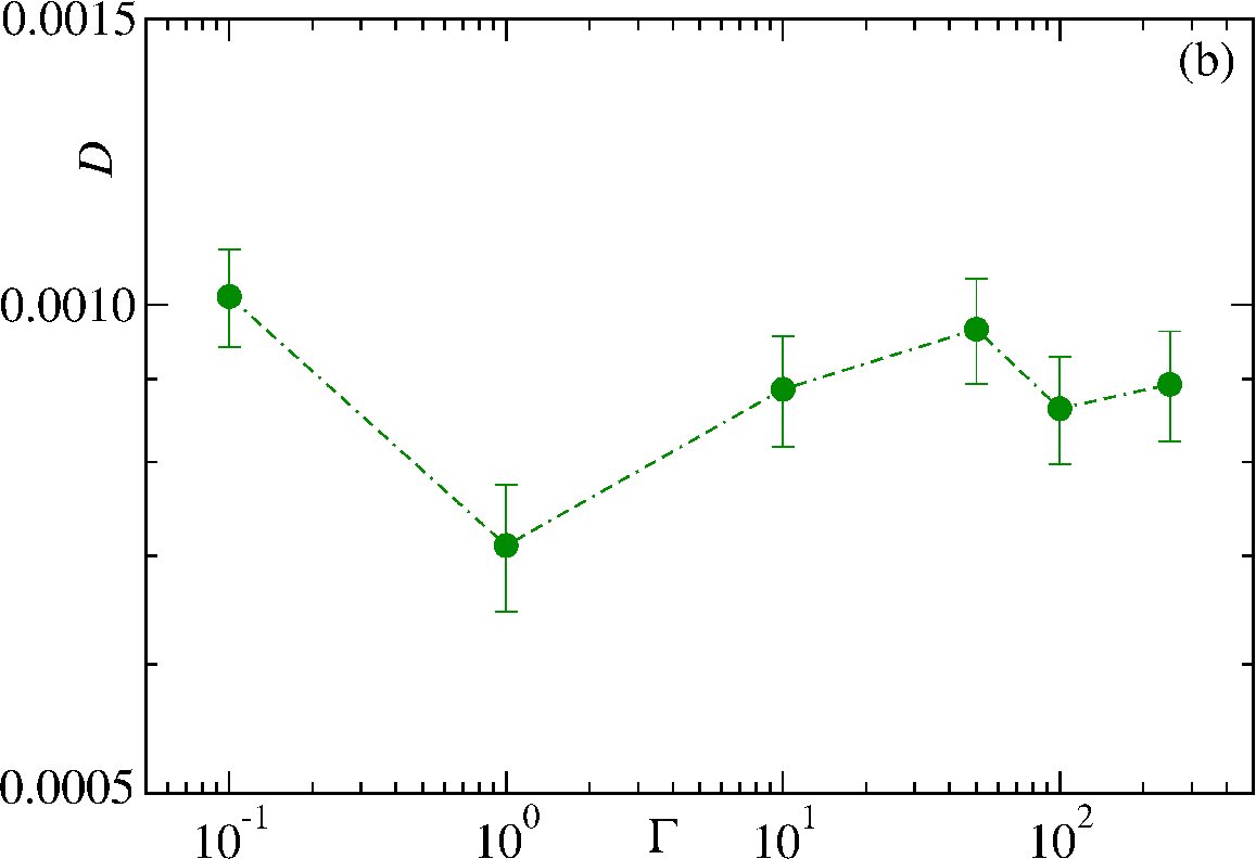
Finally, in Fig. 3(b) we show the dependence of the self-diffusion coefficient on the collision frequency that controls the effective viscosity of the solvent. The data show no signature of strong dependence, rather in a broader sense seems to be pretty constant for different . This behavior is similar to the conclusion drawn in Ref. [13] where, for an ideal gas, they did not observe any strong dependence of on . Nevertheless, the data presented here are for a relatively high temperature , hence, the influence of viscosity is not severely pronounced. At low temperatures, the diffusion might get suppressed due to high effective viscosity [15].

4 Conclusion
Motivated by dissipative particle dynamics, here, we have constructed an explicit solvent model for a polymer. Instead of using the standard approach of doing it, we rely on the Lowe-Andersen approach of the bath collision. This allows us to control the drag force applied by the solvent on the polymer, i.e., the effective viscosity. Via the scaling of the radius of gyration with the chain length as we confirm that our approach yields the known static critical exponent. The method conserves both the linear and angular momenta locally, thereby preserving the hydrodynamics. The scaling of the self-diffusion coefficient with chain length indicates a much faster dynamics than the Rouse dynamics, and in fact is pretty consistent with Zimm scaling valid in the presence of hydrodynamic effects. The successful application of this method opens up opportunities to explore other aspects of polymer dynamics including nonequilbrium scenarios, e.g., during collapse of a polymer [16, 17, 18, 19]. There, the effect of varying the collision frequency has a stronger influence on the structure formation, and in principle such phenomena could well be tuned by the degree of dissipation [20]. \ackThe work was funded by the Deutsche Forschungsgemeinschaft (DFG) under Grant Nos. JA 483/33-1 and SFB/TRR 102 (project B04), and further supported by the Deutsch-Französische Hochschule (DFH-UFA) through the Doctoral College “” under Grant No. CDFA-02-07, the EU Marie Curie IRSES network DIONICOS under Contract No. PIRSES-GA-2013-612707, and the Leipzig Graduate School of Natural Sciences “BuildMoNa”.
References
References
- [1] de Gennes P-G 1985 Scaling Concepts in Polymer Physics (Cornell University Press, Ithaca)
- [2] Doi M and Edwards S F 1986 The Theory of Polymer Dynamics (Clarendon, Oxford)
- [3] Rouse P E 1953 J. Chem. Phys. 21, 1272
- [4] Zimm B H 1956 J. Chem. Phys. 24, 269
- [5] Smith D E, Perkins T T and Chu S 1996 Macromol. 29 1372
- [6] B Dünweg and Kremer K Phys. Rev. Lett. 66 2996
- [7] Hoogerbrugge P J and Koelman J M V A 1992 Europhys. Lett. 19, 155
- [8] Espanol P and Warren P B 1995 Europhys. Lett. 30, 191
- [9] Groot R D and Warren P B 1997 J. Chem. Phys. 107, 4423
- [10] Marsh C A and Yeomans J M 1997 Europhys. Lett. 37, 511
- [11] Hafskjold B, Liew C C and Shinoda W 2004 Mol. Simul. 30, 879
- [12] Lowe C P 1999 Europhys. Lett. 47, 145
- [13] Koopman E A and Lowe C P 2006 J. Chem. Phys. 124, 204103
- [14] Plimpton S 1995 J. Comput. Phys. 117, 1; http://lammps.sandia.gov
- [15] Majumder S, Christiansen H and Janke W 2018 work in progress
- [16] de Gennes P-G 1985 J. Phys. (France) Lett. 46 639
- [17] Majumder S and Janke W 2015 Europhys. Lett. 110 58001
- [18] Majumder S, Zierenberg J and Janke W 2017 Soft Matter 13 1276
- [19] Christiansen H, Majumder S and Janke W 2017 J. Chem. Phys. 147 094902
- [20] Majumder S, Christiansen H and Janke W 2018 in preparation