跳到论文正文
W Papers独立论文阅读器 arXiv:1810.08204 论文正文 计算阅读时间 · 0%
引用这篇论文根据当前论文元数据生成,正式投稿前建议核对。


License: arXiv.org perpetual non-exclusive license
arXiv:1810.08204v2 [quant-ph] 27 May 2019

Quantum Error Correction with the Semion Code

G. Dauphinais, L. Ortiz, S. Varona, and M.A. Martin-Delgado Affiliation:  Departamento de Física Teórica, Universidad Complutense, 28040 Madrid, Spain
Abstract

We present a full quantum error correcting procedure with the semion code: an off-­shell extension of the double ­semion model. We construct open-string operators that recover the quantum memory from arbitrary errors and closed-string operators that implement the basic logical operations for information processing. Physically, the new open-string operators provide a detailed microscopic description of the creation of semions at their end­points. Remarkably, topological properties of the string operators are determined using fundamental properties of the Hamiltonian, namely, the fact that it is composed of commuting local terms squaring to the identity. In all, the semion code is a topological code that, unlike previously studied topological codes, it is of non-­CSS type and fits into the stabilizer formalism. This is in sharp contrast with previous attempts yielding non-­commutative codes.

I Introduction

Topological properties of quantum systems have become a resource of paramount importance to construct quantum memories that are more robust to external noise and decoherence Kitaev 2003; Dennis et al. 2002; Bravyi and Kitaev 1998; Bombin and Martin-Delgado 2006; Bombin and Martin-Delgado 2007a; Bombin and Martin-Delgado 2007b; Bombin and Martin-Delgado 2007c than standard quantum error correcting codes Shor 1995; Steane 1996a; Shor. 1996; E. Knill 1996; Kitaev 1997; Dorit Aharonov 1996; Nielsen and Chuang 2000; Galindo and Martín-Delgado 2002. The latter are based on a special class of codes - concatenated codes - which enable us to perform longer quantum computations reliably, as we increase the block size.

The Kitaev code is the simplest topological code yielding a quantum memory Kitaev 2003. It can be thought of as a simple two-dimensional lattice gauge theory with gauge group G=ℤ2G=\mathbb{Z}_{2}. In D=2D=2 spatial dimensions, there is another lattice gauge theory with the same gauge group but different topological properties: the Double Semion (DS) model Levin and Wen 2005; Freedman et al. 2004; Freeman and Hastings 2016; Buerschaper et al. 2014; Morampudi et al. 2014; Orús et al. 2014; Qi et al. 2015. Although the Kitaev and the DS models are lattice gauge theories sharing the same gauge group, G=ℤ2G=\mathbb{Z}_{2}, the braiding properties of their quasiparticle excitations are radically different. For example, whereas braiding two elementary quasiparticle excitations (either an electric or a magnetic charge) gives a +1+1 phase in the Kitaev code, doing so in the DS model yields ±i\pm i phase factors.

The DS model was introduced in the context of the search of new topological orders in strongly correlated systems, gapped, non-chiral and based on string-net mechanisms in D=2D=2 dimensions Levin and Wen 2005; Freedman et al. 2004. Generalizations of the DS model to D=3D=3 and to higher dimensions have appeared recently Freeman and Hastings 2016. While the properties of the Kitaev code has been extensively studied in quantum computation and condensed matter, barely nothing is known about the quantum error correcting properties of the DS model despite recent efforts towards realizing such models Furusaki 2017; Li et al. 2017; Syed et al. 2019. In this work we remedy this situation by introducing a new formulation of the DS model that is suitable for a complete treatment as a quantum memory with topological properties.

The first obstacle to tackle the DS model as a quantum memory is the original formulation as a string-net model Levin and Wen 2005. In this formulation, the Hamiltonian is only Hermitian and exactly solvable in a particular subspace, where plaquette operators are Hermitian and commute. Only linear combinations of closed-string configurations, implying the absence of vertex excitations, are allowed in this subspace Levin and Wen 2005; Mesaros and Ran 2013; von Keyserlingk et al. 2013. The microscopic formulation of the original DS model starts with a hexagonal lattice Λ\Lambda with qubits placed at links ee. Vertex operators QvQ_{v} are attached to the three links meeting at a vertex v∈Λv\in\Lambda. Plaquette operators B~p\tilde{B}_{p} are attached to hexagons p∈Λp\in\Lambda with the novel feature that their outer links carry additional phase factors that are missing in the corresponding Kitaev model. Explicitly,

Qv:=σiz​σjz​σkz,Q_{v}:=\sigma^{z}_{i}\sigma^{z}_{j}\sigma^{z}_{k}, (1)

with i,j,ki,\ j,\ k, being the three qubits belonging to vertex vv (see Fig. 1a) and

B~p:=(∏i∈∂pσix)​∏j∈o⁡(p)i12​(1−σjz),\tilde{B}_{p}:=\left(\prod_{i\in\partial p}\sigma^{x}_{i}\right)\prod_{j\in o(p)}i^{\frac{1}{2}\left(1-\sigma^{z}_{j}\right)}, (2)

where ∂p\partial p are the six links of the hexagon and o⁡(p)o(p) is the set of six edges outgoing from each plaquette pp, as it is shown in Fig. 1b. Unlike the Kitaev code, these plaquette operators B~p\tilde{B}_{p} are Hermitian and commute among themselves only in a subspace of the whole Hilbert space, defined by the so-called zero-flux rule Levin and Wen 2005; Mesaros and Ran 2013; von Keyserlingk et al. 2013. This is given by a vertex-free condition on states,

ℋv:={|ψ⟩:Qv|ψ⟩=+|ψ⟩,∀v∈Λ}.{\cal H}_{v}:=\{|\psi\rangle:Q_{v}|\psi\rangle=+|\psi\rangle,\forall v\in\Lambda\}. (3)

Refer to caption

(a)
Refer to caption
(b)
Figure 1: The support of the vertex operator Qv=σ1z​σ2z​σ3zQ_{v}=\sigma^{z}_{1}\sigma^{z}_{2}\sigma^{z}_{3} and plaquette operator B~p\tilde{B}_{p}. The qubits are placed on the edges.

The set of vertex and plaquette operators defines a Hamiltonian

H~DS:=−∑v∈ΛQv+∑p∈ΛB~p.\tilde{H}_{\mathrm{DS}}:=-\sum_{v\in\Lambda}Q_{v}+\sum_{p\in\Lambda}\tilde{B}_{p}. (4)

Due to the involved structure of phases that plaquette operators in Eq. (2) have, it was aforementioned that these operators do not commute out of the vertex-free subspace. This implies that the model is only well-defined when there are no vertex excitations.

Therefore, in order to treat the DS model as a quantum error correcting code Calderbank and Shor 1996; Steane 1996b; Preskill 2004; E. Knill 1996; Terhal 2015, it is necessary to have a formulation of the model that is valid in the whole Hilbert space and not just for the vertex-free subspace (3), since generic noise processes will make the system leave the mentioned subspace. To this end, we introduce an off-shell DS model that we call the semion code. This new model is achieved by making a deformation of the original plaquette operators (2) such that they become commuting and Hermitian operators without imposing the vertex-free condition von Keyserlingk et al. 2013. In addition, we are able to develop the complete program of quantum error correction with the semion code.

I.1 Summary of main results

In order to summarize the main contributions that we present in this paper, we hereby advance a list of some of our most relevant results.

  1. (i)

    We perform a thorough analysis of a formulation of the plaquette operators which commute in the whole Hilbert space von Keyserlingk et al. 2013. This construction consists in adding extra phases to the plaquette operators, which depend on the configuration of the three edges at each vertex. When the vertex-free condition is imposed, we recover the standard definition of the DS model.

  2. (ii)

    We give an explicit construction for string operators along arbitrary paths. They are complete in the sense that any operator acting on the system can be decomposed as a linear superposition of such operators. Additionally, the string operators can be constructed efficiently despite the complex structure of the plaquette operators. Remarkably, a microscopic formulation to create semions was not proven until now.

  3. (iii)

    We analytically show that the excitations of the system behave as semions, via the detailed study of the constructed string operators, which allows us to explicitly calculate the topological S-matrix. Interestingly enough, most of the string operator properties rely on very generic arguments about the structure of the local operators making up the Hamiltonian, namely that they commute and square to the identity.

  4. (iv)

    Closed-string operators are constructed, which allow us to perform logical operations on the quantum memory built from the semion code. Logical operators are closed-string operators whose paths are homologically non-trivial and act non-trivially on the degenerate ground space.

  5. (v)

    Given the above properties, we define a topological quantum error correcting code based on a non-trivial extension of the DS model. We build a code, which is characterized by the following key properties: is topological, satisfies the stabiliser formalism, is non-CSS, non-Pauli and additive.

The topological nature of the code becomes apparent through the fact that global degrees of freedom are used to encode information and only local interactions are considered Kitaev 2003; Bombin and Martin-Delgado 2006. Another remarkable feature of the semion code is that is of non-CSS type since in the plaquette operators both Pauli XX and ZZ operators enter in the definition Calderbank and Shor 1996; Steane 1996a. Consequently, errors in an uncorrelated error model such as independent bit-flip and phase-flip errors cannot be treated separately. However, they can be decomposed as a linear superpositions of fundamental anyonic errors (string operators creating pairs of anyons) with a known effect on the Hilbert space. Moreover, the semion code is not a subgroup of the Pauli group since the complex phases entering its definition (see Eq. (2)) makes impossible to express its generators in terms of tensor products of Pauli matrices Gottesman 1996; Ni et al. 2015. Nevertheless, the semion code is still an additive code: the sum of quantum codewords is also a codeword Calderbank et al. 1997. This last fact is intimitely related to the abelian nature of the semionic excitations Kitaev 2006; Pfeifer et al. 2012.

I.2 Outline

The article is organized as follows. In Sec. II we introduce the off-shell DS model, which is suitable for quantum error correction. In Sec. III we build string operators creating vertex excitations at their endpoints. Sec. IV is devoted to logical operators and quantum error correction. We conclude in Sec. V. Appendices deserve special attention since they contain the detailed explanations of all the constructions used throughout the text. Specifically, App. A presents an explicit example of a string operator, App. B gives the detailed proof of Theorem 1, which presents a systematic way to construct string operators, as well as several key properties of the string operators and finally App. C is devoted to the proof of Theorem 2, which gives the commutation relations among string operators.

II Off-Shell double semion: microscopic model

We begin by considering a microscopic description of the DS model on the entire Hilbert space of states, since it is much better suited for quantum error correction. We call this an off-shell DS code by borrowing the terminology from quantum field theory and other instances in physics where a shell condition amounts to a constraint on the phase space of a system. For instance, the equation of motion is a shell condition for quantum particles but the phase space is more general. In our case, the shell condition is the vertex-free subspace or zero-flux rule introduced in Eq. (3).

II.1 Double semion model in the vertex-free subspace

Let us start by introducing the DS model in a new presentation that is more suitable for building an off-shell formulation of it. We consider the same hexagonal lattice Λ\Lambda with qubits attached to the edges e∈Λe\in\Lambda. The vertex operators QvQ_{v} will remain the same as in Eq. (1), but the plaquette operators in the zero-flux subspace can be rewritten in an equivalent form to that shown in Eq. (2), i.e.,

B~p=(∏j=16σjx)​(∏j=16(−1)nj−1−​nj+),\tilde{B}_{p}=\left(\prod_{j=1}^{6}\sigma^{x}_{j}\right)\left(\prod_{j=1}^{6}\left(-1\right)^{n^{-}_{j-1}n^{+}_{j}}\right), (5)

in which ni±:=12​(1±σiz)n^{\pm}_{i}:=\frac{1}{2}(1\pm\sigma^{z}_{i}) is the projector on the state |0⟩|0\rangle (n+n^{+}) or |1⟩|1\rangle (n−n^{-}) of qubit ii, qubits are labeled as shown in Fig. 1 and we use the convention that n0±n^{\pm}_{0} refers to qubit ‘6’ for simplicity. Remarkably, this expression avoids any reference to the outgoing links of hexagonal plaquettes pp. One readily sees that the vertex operators fulfill the following relations:

Qv2=1,[Qv,Qv′]=0,[Qv,B~p]=0;Q^{2}_{v}=1,\quad[Q_{v},Q_{v^{\prime}}]=0,\quad[Q_{v},\tilde{B}_{p}]=0; (6)

∀v,v′,p∈Λ\forall v,v^{\prime},p\in\Lambda. As for the plaquette operators B~p\tilde{B}_{p}, they also satisfy

B~p2=1,B~p†=B~p,[B~p,B~p′]=0;\tilde{B}^{2}_{p}=1,\quad\tilde{B}^{\dagger}_{p}=\tilde{B}_{p},\quad[\tilde{B}_{p},\tilde{B}_{p^{\prime}}]=0; (7)

∀p,p′∈Λ\forall p,p^{\prime}\in\Lambda, but only in the vertex-free subspace (3). Furthermore, the product of all the vertex and plaquette operators is the identity. A simple counting argument reveals that the ground space is 4g4^{g} degenerate11 1 This is strictly true only if the total number of plaquettes of the system is even. If it is odd, then the ground state must contain a single flux excitation, which can be placed in any of the plaquettes. In that latter case the ground space degeneracy is an extensive quantity. However, any given flux configuration is 4g4^{g}-degenerate. For simplicity, we assume in this work that the system contains an even number of plaquettes., which gg being the genus of the orientable compact surface onto which the lattice is placed.

An explicit unnormalized wavefunction belonging to the ground space is obtained in the following way: we start from the vacuum, i.e., |0⟩⊗N|0\rangle^{\otimes N}, which has +1 eigenvalue for all vertex operators. Then, plaquette operators are used to build projectors and apply them onto the vacuum,

|Ω⟩=∏p∈Λ1−B~p2​|0⟩⊗N.\displaystyle|\Omega\rangle=\prod_{p\in\Lambda}\frac{1-\tilde{B}_{p}}{2}\ |0\rangle^{\otimes N}. (8)

It is straightforward to check that this state fulfills the lowest energy condition for the Hamiltonian (4) within the vertex-free subspace. Expanding the product in Eq. (8), one can see that the ground state is a superposition of closed loops configurations. Due to the condition B~p=−1\tilde{B}_{p}=-1 for the ground state, the coefficients of this superposition of closed loops alternate sign. Thus, we can write the ground state in a different way:

|Ω⟩=∑i→∈{C-S conf.}(−1)NL​(i→)​|i→⟩,\displaystyle|\Omega\rangle=\sum_{\vec{i}\ \in\left\{\text{C-S conf.}\right\}}(-1)^{N_{L}\left(\vec{i}\right)}|\vec{i}\;\rangle, (9)

where i→\vec{i} is a bitstring representing a qubit configuration and {C-S conf.}\left\{\text{C-S conf.}\right\} is the set of all possible closed-string configurations. Each configuration in this set has a certain number of closed loops, NL​(i→)N_{L}(\vec{i}), whose parity determines the sign of the coefficient in the ground state superposition.

Of course the above construction only gives rise to one of the ground states. To find the other ones, the starting configuration can simply be replaced by a configuration containing an homologically non-trivial closed loop (which necessarily belongs to the vertex-free subspace), and proceed with the same construction. Every different homological class for the closed loop corresponds to a different ground state.

Applying the B~p\tilde{B}_{p} operator on a specific loop configuration flips the string occupancy of the interior edges of plaquette pp while acquiring a phase that depends on the specific configuration under consideration. Applying B~p\tilde{B}_{p} on the vacuum simply adds a closed loop around plaquette pp, while applying B~p\tilde{B}_{p} next to a closed loop either enlarges (or shrinks) the existing loop to include (exclude) plaquette pp, while multiplying the wave function by −1-1 factor (see Fig. 2).

Refer to caption
Figure 2: Applying plaquette operator B~q\tilde{B}_{q} adds a closed loop around plaquette qq and multiply the wave function by a −1-1 phase. Each qubit in a given configuration is represented by a filled link of the lattice if it is in state |1⟩|1\rangle, whereas links in |0⟩|0\rangle are left empty (dashed line).

Due to the lack of commutativity of the plaquette operators and the fact that they are not Hermitian, the original DS model is only well-defined when there are no vertex excitations. Moreover, the strings creating vertex excitations are not properly defined either. A naive attempt to construct these strings as a chain of σx\sigma^{x} operators, following the similarities with the Kitaev code, resoundingly fails. As a consequence of the phases on the external legs of plaquette operators, σx\sigma^{x} operators create vertex excitations but also plaquette excitations. In order to get a string that creates only two vertex excitations at the endpoints but commutes with all the plaquette operators along the path 𝒫\mathcal{P}, it is necessary to add some extra phases to the chain of σx\sigma^{x} on the outer legs. An approach to this problem is described in von Keyserlingk et al. 2013 but it is not successfully solved since the strings are only well-defined in the vertex-free subspace.

The DS model gives rise to quasiparticle excitations behaving like anyons. They are called semions, due to the fact that their topological charge is ‘half’ of that of a fermion, i.e., ±i\pm i. There exist two types of semions in the model, one corresponding to a vertex excitation, while the other corresponds to both vertex and adjacent plaquettes excitations. From now on, we name these two different possibilities as chiralities, positive chirality for the former kind, and negative chirality for the latter one. We warn the reader that this choice has been made arbitrarily, and does not necessarily reflect the topological charge of a given specie.

Taking into account all these caveats, we present in the following a formulation of the DS model which gives a microscopic approach to this interesting topological order, fulfilling all the necessary properties in the whole Hilbert space.

II.2 Exactly solvable model in the whole Hilbert space

If we want to consider encoding quantum information in the degenerate ground-state manifold of the standard (on-shell) DS model in Eq. (4), we immediately run into major problems: XX Pauli errors make the state of the system leave the vertex-free subspace. The non-commutativity of the B~p\tilde{B}_{p} operators poses difficulties when interpreting the DS model as a stabilizer code.

To avoid such difficulties, we consider a modified version of the plaquette operators in Eq. (2), which we call the off-shell DS model or semion code

HDS=−∑vQv+∑pBp,H_{\rm{DS}}=-\sum_{v}Q_{v}+\sum_{p}B_{p}, (10)

where the generalized plaquette operator BpB_{p} is a modification of B~p\tilde{B}_{p} obtained by multiplying it by a phase factor that depends on the configuration on which it is applied. More specifically, we have

Bp:=B~p×β~p,B_{p}:=\tilde{B}_{p}\times\tilde{\beta}_{p}, (11)

with

β~p:=∑i→b~p​(i→)​|i→⟩​⟨i→|,\tilde{\beta}_{p}:=\sum_{\vec{i}}\tilde{b}_{p}(\vec{i})|\vec{i}\rangle\langle\vec{i}|, (12)

where the sum runs over all possible configurations of edges 11 through 1212 shown in Fig. 1. b~p​(i→)\tilde{b}_{p}(\vec{i}) is the phase factor corresponding to the string configuration i→\vec{i}. i→\vec{i} represents a state in the computational basis. A qubit in the state |0⟩|0\rangle is interpreted as the absence of a string on its corresponding edge, while the state |1⟩|1\rangle reflects the presence of a string. The phase operator βp\beta_{p} can be decomposed as

β~p=β(6,1,12)​β(1,2,7)​β(2,3,8)​β(3,4,9)​β(4,5,10)​β(5,6,11),\tilde{\beta}_{p}=\beta_{(6,1,12)}\,\beta_{(1,2,7)}\,\beta_{(2,3,8)}\,\beta_{(3,4,9)}\,\beta_{(4,5,10)}\,\beta_{(5,6,11)}, (13)

where β(i,j,k)\beta_{(i,j,k)} is a function of the string configuration of edges i,ji,j and kk connected to vertex v⁡(i,j,k)v(i,j,k). The specific values for each factor β(i,j,k)\beta_{(i,j,k)} are shown graphically in Fig. 3. Note that their specific form differ depending on their position on the plaquette.

For future reference, notice that the generalised plaquette operator BpB_{p} can be written as

Bp=∏i∈∂pσix​(∏j∈∂p(−1)nj−1−​nj+)​∏v∈pβv,B_{p}=\prod_{i\in\partial p}\sigma^{x}_{i}\left(\prod_{j\in\partial p}\left(-1\right)^{n^{-}_{j-1}n^{+}_{j}}\right)\prod_{v\in p}\beta_{v}, (14)

where we use the notation j∈∂pj\in\partial p to indicate the qubit associated to edge jj in plaquette pp. v∈pv\in p identify the vertices belonging to plaquette pp. Notice that this last expression clearly shows that the phase factor appearing in BpB_{p} is a product of phases, βv\beta_{v}, depending on the string configuration of the three edges connected to each vertex of plaquette pp. The complete algebraic expression of the product of all βv\beta_{v} in a plaquette pp is von Keyserlingk et al. 2013

∏v∈pβv\displaystyle\prod_{v\in p}\beta_{v} =in12−​(n1−​n6−−n1+​n6+)​in7−​(n1+​n2+−n1−​n2−)\displaystyle=\ i^{n_{12}^{-}\left(n^{-}_{1}n^{-}_{6}-n^{+}_{1}n^{+}_{6}\right)}i^{n^{-}_{7}\left(n^{+}_{1}n^{+}_{2}-n^{-}_{1}n^{-}_{2}\right)}
×in8+​(n2−​n3+−n2+​n3−)​in9−​(n3−​n4−−n3+​n4+)\displaystyle\times\ i^{n^{+}_{8}\left(n^{-}_{2}n^{+}_{3}-n^{+}_{2}n^{-}_{3}\right)}i^{n^{-}_{9}\left(n^{-}_{3}n^{-}_{4}-n^{+}_{3}n^{+}_{4}\right)} (15)
×in10−​(n4+​n5+−n4−​n5−)​in11+​(n5−​n6+−n5+​n6−).\displaystyle\times\ i^{n^{-}_{10}\left(n^{+}_{4}n^{+}_{5}-n^{-}_{4}n^{-}_{5}\right)}i^{n^{+}_{11}\left(n^{-}_{5}n^{+}_{6}-n^{+}_{5}n^{-}_{6}\right)}.

We can easily check that in the zero-flux rule the factors in Eq. (II.2) reduce to 1, recovering expression (5) for the plaquette operators.

The crucial point now is that the new generalized plaquette operators, BpB_{p}, satisfy the desired properties needed by the stabilizer formalism of quantum error correction. Namely,

Bp2=1,Bp†=Bp,[Bp,Bp′]=0,[Qv,Bp]=0;B^{2}_{p}=1,\ \ B^{\dagger}_{p}=B_{p},\ \ [B_{p},B_{p^{\prime}}]=0,\ \ [Q_{v},B_{p}]=0; (16)

∀p,p′,v∈Λ,\forall p,\ p^{\prime},\ v\in\Lambda, regardless of the vertex-free condition (3). The study of HDSH_{\rm{DS}} is rendered much simpler than that of H~DS\tilde{H}_{\rm{DS}} on the whole Hilbert space of the qubits by the fact that the new plaquette operators commute.

Figure 3: A graphical representation of the various non-trivial phase factors of the form β(i,j,k)\beta_{(i,j,k)}. A trivial phase of +1+1 is applied for any configuration not shown on this picture. The labeling of the edges have been omitted for simplicity, and corresponds to the same as the one on Fig. 1.

III String operators

We seek open-string operators creating excitations at their endpoints without affecting the rest of vertex and plaquette operators, as well as closed-string operators that commute with vertex and plaquette operators. In our case, excited states correspond to states in a −1-1 eigenstate for a vertex operator or a +1+1 eigenstate of a plaquette operator. We say that an excitation is present at vertex vv (plaquette pp) if the state of the system is in a −1-1 (+1+1) eigenstate of QvQ_{v} (BpB_{p}). Since we have that ∏v∈ΛQv=∏p∈ΛBp=1\prod_{v\in\Lambda}Q_{v}=\prod_{p\in\Lambda}B_{p}=1, excitations are always created in pairs.

In order to find such string operators, it is convenient to reexpress the generalized plaquette operators as

Bp=∏i∈pσix​∑i→bp​(i→)​|i→⟩​⟨i→|,B_{p}=\prod_{i\in p}\sigma^{x}_{i}\sum_{\vec{i}}b_{p}\left(\vec{i}\right)|\vec{i}\rangle\langle\vec{i}|, (17)

where pp denotes the interior edges of a plaquette (edges 11 through 66 in Fig. 1) and the string configurations in the sum are taken on edges 11 through 1212. bp​(i→)b_{p}(\vec{i}) denotes the complex phase picked up when applying operator BpB_{p} to the configuration i→\vec{i}. Note that ∑i→bp​(i→)​|i→⟩​⟨i→|\sum_{\vec{i}}b_{p}(\vec{i})|\vec{i}\rangle\langle\vec{i}| differs from the product of the βp\beta_{p}’s in the −1-1 factors appearing in Eq. (14). ∑i→bp​(i→)​|i→⟩​⟨i→|\sum_{\vec{i}}b_{p}(\vec{i})|\vec{i}\rangle\langle\vec{i}| includes the −1-1 factors as well as the product of βv\beta_{v}.

Given two string configurations i→\vec{i} and α→\vec{\alpha} on a set of edges, it is useful to define the string configuration i→⊕α→\vec{i}\oplus\vec{\alpha} to be the configuration i→′\vec{i}^{\prime} where the edges occupied in configuration α→\vec{\alpha} has been flipped. It is equivalent to sum (mod 2) the two bitstrings. Additionally, we define the configuration α→p\vec{\alpha}^{p} of plaquette pp as the string configuration which is empty everywhere except for the six edges in the interior of plaquette pp, corresponding to edges 11 through 66 in Fig. 1. Likewise, α→𝒫\vec{\alpha}^{\mathcal{P}}, will be the configuration which is only occupied for edges of path 𝒫\mathcal{P}.

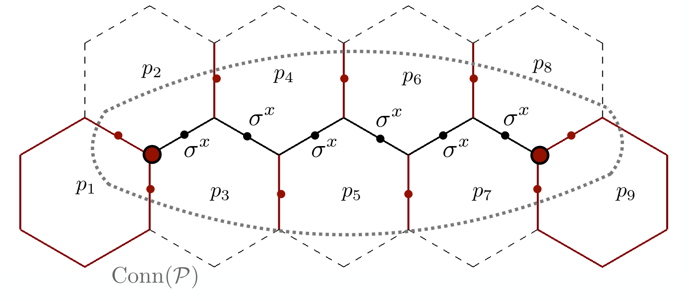
Given a path 𝒫\mathcal{P}, we construct string operators S𝒫+S^{+}_{\mathcal{P}} creating vertex excitations at its endpoints and commuting with every other operators in Hamiltonian (10). Negative chirality strings are defined as S𝒫−:=S𝒫+​S𝒫dual′zS^{-}_{\mathcal{P}}:=S^{+}_{\mathcal{P}}S^{z}_{\mathcal{P^{\prime}_{\textnormal{dual}}}}, where S𝒫dual′zS^{z}_{\mathcal{P^{\prime}_{\textnormal{dual}}}} is a product of σz\sigma^{z} operators forming a path 𝒫dual′\mathcal{P^{\prime}_{\textnormal{dual}}} in the dual lattice which is contained in the support of S𝒫+S^{+}_{\mathcal{P}}. If 𝒫\mathcal{P} is open, S𝒫dual′zS^{z}_{\mathcal{P^{\prime}_{\textnormal{dual}}}} creates excitations at plaquettes containing the vertices at the endpoints of 𝒫\mathcal{P} and opposite to the first and last edges of 𝒫\mathcal{P} (p1p_{1} and p9p_{9} in Fig. 4), while if 𝒫\mathcal{P} is closed, S𝒫dual′zS^{z}_{\mathcal{P^{\prime}_{\textnormal{dual}}}} forms a closed path in the same homological class as 𝒫\mathcal{P}. Note that for a given path 𝒫\mathcal{P}, various paths 𝒫dual′\mathcal{P}^{\prime}_{\textnormal{dual}} are possible, and each one gives rise to a different string operator S𝒫−S^{-}_{\mathcal{P}}.

III.1 An algorithm to generate string operators

In order to find these string operators, we consider the following ansatz:

S𝒫+:=∏i∈𝒫σix​∑i→∈Conn​(𝒫)F𝒫​(i→)​|i→⟩​⟨i→|,S^{+}_{\mathcal{P}}:=\prod_{i\in\mathcal{P}}\sigma^{x}_{i}\sum_{\vec{i}\,\in\,\textnormal{Conn}(\mathcal{P})}F_{\mathcal{P}}\left(\vec{i}\right)|\vec{i}\rangle\langle\vec{i}|, (18)

where F𝒫​(i→)F_{\mathcal{P}}(\vec{i}) is a phase factor acquired when S𝒫+S^{+}_{\mathcal{P}} is applied on configuration i→\vec{i}. F𝒫​(i→)F_{\mathcal{P}}(\vec{i}) only depends on qubits belonging to Conn​(𝒫)\textnormal{Conn}(\mathcal{P}), defined as:

Conn​(𝒫):={links of​𝒫​ and its external legs}.\textnormal{Conn}(\mathcal{P}):=\{\textnormal{links of}\;\mathcal{P}\textnormal{ and its external legs}\}. (19)

It is also useful to define the set of plaquettes

ℬ𝒫:={p:∂p∩Conn​(𝒫)≠∅},\mathcal{B}_{\mathcal{P}}:=\{p:\partial p\;\cap\;\textnormal{Conn}(\mathcal{P})\neq\varnothing\}, (20)

which is the set of plaquettes that have at least one of their interior edges contained in Conn(𝒫\cal{P}). Equivalently, one can define ℬ𝒫\mathcal{B}_{\mathcal{P}} to be the set of plaquettes such that for at least one string configuration i→\vec{i}, bp​(i→⊕α→𝒫)≠bp​(i→)b_{p}(\vec{i}\oplus\vec{\alpha}^{\mathcal{P}})\neq b_{p}(\vec{i}). The structure of S𝒫+S^{+}_{\mathcal{P}} is illustrated in Fig. 4. Note that depending on the context, a configuration i→\vec{i} is either understood to be on the full system, or is the configuration restricted to Conn​(𝒫)\textnormal{Conn}(\mathcal{P}). The specific case considered is explicitly stated in each case.

Ansatz (18) should satisfy the following properties:

  1. (i)

    Anticommutes with vertex operators at the endpoints of 𝒫\cal{P} if it is open, while it commutes with every other vertex and plaquette operators.

  2. (ii)

    Acts trivially on edges outside Conn(𝒫\cal{P}).

Operators satisfying (i) and (ii) are called string operators. Additionally, we may be interested in the properties:

  1. (iii)

    Squares to the identity.

  2. (iv)

    Hermitian.

If these are satisfied, they will be called canonical string operators.
Properties (iii) and (iv) are satisfied (see Lemmas 5 and 6 in App. B) if

F𝒫​(i→⊕α→𝒫)=[F𝒫​(i→)]∗.F_{\mathcal{P}}\left(\vec{i}\oplus\vec{\alpha}^{\mathcal{P}}\right)=\left[F_{\mathcal{P}}\left(\vec{i}\right)\right]^{*}. (21)
Refer to caption
Figure 4: The structure of S𝒫+S^{+}_{\mathcal{P}}, where the path 𝒫\mathcal{P} is indicated by the full black edges where the σx\sigma^{x} operators are applied. The phase factors F𝒫+F^{+}_{\mathcal{P}} depend on the configuration of all the edges identified with a dot, which are collectively denoted by Conn​(𝒫)\textnormal{Conn}(\mathcal{P}). The effect of S𝒫+S^{+}_{\mathcal{P}} on the ground state of the system is to create a pair of vertex excitations at the vertices located at the endpoints of the path 𝒫\mathcal{P}, which are identified by big red dots. Plaquettes p1p_{1} to p9p_{9} constitute the set ℬ𝒫\mathcal{B}_{\mathcal{P}}.

Since we want S𝒫+S^{+}_{\mathcal{P}} to commute with all plaquettes in ℬ𝒫\mathcal{B}_{\mathcal{P}} (for the rest of plaquettes, it commutes by construction), we impose that the commutator vanishes, [S𝒫+,Bp]=0\left[S^{+}_{\mathcal{P}},B_{p}\right]=0, which yields the equation

F𝒫​(i→⊕α→p)=bp​(i→⊕α→𝒫)bp​(i→)​F𝒫​(i→).F_{\mathcal{P}}\left(\vec{i}\oplus\vec{\alpha}^{p}\right)=\frac{b_{p}\left(\vec{i}\oplus\vec{\alpha}^{\mathcal{P}}\right)}{b_{p}\left(\vec{i}\right)}F_{\mathcal{P}}\left(\vec{i}\right). (22)

It is useful to define the function θ𝒫​(i→,p):=bp​(i→⊕α→𝒫)/bp​(i→)\theta_{\mathcal{P}}(\vec{i},p):={b_{p}(\vec{i}\oplus\vec{\alpha}^{\mathcal{P}})}/{b_{p}(\vec{i})}, which relates F𝒫​(i→⊕α→p)F_{\mathcal{P}}(\vec{i}\oplus\vec{\alpha}^{p}) to F𝒫​(i→)F_{\mathcal{P}}(\vec{i}). We can generalize Eq. (22) and function θ𝒫​(i→,p)\theta_{\mathcal{P}}(\vec{i},p) for an arbitrary number of plaquettes, namely,

F𝒫​(i→⊕α→p1⊕…⊕α→pm)=θ𝒫​(i→,p1,…,pm)​F𝒫​(i→),F_{\mathcal{P}}\left(\vec{i}\oplus\vec{\alpha}^{p_{1}}\oplus...\oplus\vec{\alpha}^{p_{m}}\right)=\theta_{\mathcal{P}}\left(\vec{i},p_{1},...,p_{m}\right)F_{\mathcal{P}}\left(\vec{i}\right), (23)

where θ𝒫​(i→,p1,…,pm)\theta_{\mathcal{P}}(\vec{i},p_{1},...,p_{m}) can be expressed as

θ𝒫​(i→,p1,…,pm)=∏i=1mbpi​(i→⊕α→𝒫​⨁j=1i−1α→pj)bpi​(i→​⨁j=1i−1α→pj).\theta_{\mathcal{P}}\left(\vec{i},p_{1},\dots,p_{m}\right)=\prod_{i=1}^{m}\frac{b_{p_{i}}\left(\vec{i}\oplus\vec{\alpha}^{\mathcal{P}}\bigoplus\limits_{j=1}^{i-1}\vec{\alpha}^{p_{j}}\right)}{b_{p_{i}}\left(\vec{i}\bigoplus\limits_{j=1}^{i-1}\vec{\alpha}^{p_{j}}\right)}. (24)

Note that while we use the same symbol for the configurations i→\vec{i} in θ𝒫\theta_{\mathcal{P}} and in F𝒫F_{\mathcal{P}}, the one in θ𝒫\theta_{\mathcal{P}} is over the whole system in order for Eq. (24) to be well-defined. The specific way that the configuration i→\vec{i} is extended over the whole system (i.e which configuration on the rest of the system is appended to it) does not matter, since as a consequence of the structure of the plaquette operators, it does not affect the value of θ𝒫\theta_{\mathcal{P}}. As a consequence of the fact that plaquette operators commute, the order of the plaquettes p1,…,pmp_{1},\ ...,\ p_{m} in θ𝒫​(i→,p1,…,pm)\theta_{\mathcal{P}}(\vec{i},p_{1},...,p_{m}) does not matter (see Lemma 1). The function θ𝒫​(i→,p1,…,pm)\theta_{\mathcal{P}}(\vec{i},p_{1},...,p_{m}) relates the value of F𝒫F_{\mathcal{P}} for configuration i→\vec{i} to that of configuration i→⊕α→p1⊕…⊕α→pm\vec{i}\oplus\vec{\alpha}^{p_{1}}\oplus...\oplus\vec{\alpha}^{p_{m}}. These two configurations differ by a sum of plaquettes and may be considered part of the same configuration class 𝒞𝒫​(i→)\mathcal{C}_{\mathcal{P}}\left(\vec{i}\right), defined as

𝒞𝒫​(i→):={j→:j→=i→​⨁p∈subset⁡(ℬ𝒫)α→p},\mathcal{C}_{\mathcal{P}}\left(\vec{i}\right):=\left\{\vec{j}:\vec{j}=\vec{i}\bigoplus_{p\in\rm{subset}(\mathcal{B}_{\mathcal{P}})}\vec{\alpha}^{p}\right\}, (25)

where the configurations are restricted to Conn​(𝒫)\textnormal{Conn}(\mathcal{P}). These configurations can be regarded as the set of configurations related to i→\vec{i} by adding loops associated with plaquettes in ℬ𝒫\mathcal{B}_{\mathcal{P}}, only in the region where S𝒫+S^{+}_{\mathcal{P}} acts non-trivially. Taking all this into account, one can obtain an algorithm to compute the phases F𝒫+F^{+}_{\mathcal{P}} of the ansatz in Eq. (18). This is given by Algorithm 1.

for every configuration class 𝒞𝒫\mathcal{C}_{\mathcal{P}} do
 Pick a class representative i→∈𝒞𝒫\vec{i}\in\mathcal{C}_{\mathcal{P}}
 Set F𝒫​(i→)=ei​ϕ​(i→)F_{\mathcal{P}}(\vec{i})=e^{i\phi(\vec{i})}  
 for every subset (p1,…,pm)⊆ℬ𝒫(p_{1},\dots,p_{m})\subseteq\mathcal{B}_{\mathcal{P}} do
  F𝒫​(i→​⨁i=1mα→pi)=θ𝒫​(i→,p1,…,pm)​F𝒫​(i→)F_{\mathcal{P}}(\vec{i}\bigoplus\limits_{i=1}^{m}\vec{\alpha}^{p_{i}})=\theta_{\mathcal{P}}(\vec{i},p_{1},\dots,p_{m})F_{\mathcal{P}}(\vec{i})  
 end for
end for
List of Algorithms 1 Determination of the F𝒫F_{\mathcal{P}} functions for a path 𝒫\mathcal{P}. ei​ϕ​(i→)e^{i\phi(\vec{i})} are initial phases that can take any value.

Algorithm 1 begins by picking up a configuration i→\vec{i}, which we call its class representative, and by setting its value to an arbitrary phase ei​ϕ​(i→)e^{i\phi(\vec{i})}. Any phase picked up by the algorithm yields a valid string operator. Once the value for the class representative i→\vec{i} is fixed, the algorithm assigns values to the rest of the configurations in the same configuration class by making use of Eq. (23). Afterwards, a configuration, belonging to a different configuration class, where the values have not yet been fixed, is chosen and the same procedure is repeated until F𝒫F_{\mathcal{P}} has been fixed for all possible configurations. An explicit example of this can be seen in App. A.

As it is shown in App. B, it is always possible to determine F𝒫F_{\mathcal{P}} using Algorithm 1 such that the resulting S𝒫+S^{+}_{\mathcal{P}} is a string operator. Furthermore, it is also possible to enforce the constraint given in Eq. (21) such that we obtain canonical string operators. Those important results are summarized in the following theorem:

Theorem 1.

Let 𝒫\mathcal{P} be a path. Any function F𝒫F_{\mathcal{P}} defined by Algorithm 1 is such that S𝒫+S^{+}_{\mathcal{P}} is a string operator. Furthermore, it is possible to choose the phases ei​ϕe^{i\phi} such that the string operator is canonical.

Note that the open-string operators generated by Algorithm 1, S𝒫+S^{+}_{\mathcal{P}}, have positive chirality, because they anticommute with vertex operators at the endpoints of 𝒫\mathcal{P} and commute with every other vertex and plaquette operators, satisfying property (i). However, the same does not apply to closed-string operators, since closed strings do not have endpoints. Algorithm 1 produces, in general, closed-string operators without a definite chirality.

III.1.1 Concatenation of open-string operators

It is very useful to build strings as a concatenation of smaller strings. This is specially relevant for constructing non-trivial closed strings, since, as it was mentioned before, Algorithm 1 yields, in general, closed strings which have no definite chirality. By building these closed strings out of a multiplication of open strings, which have definite chirality, we obtain positive- and negative-chirality closed strings. Observe that given two paths, 𝒫1\mathcal{P}_{1} and 𝒫2\mathcal{P}_{2}, meeting at one endpoint or forming a closed path, the multiplication of both S𝒫1​#​𝒫2+=S𝒫2+​S𝒫1+S^{+}_{\mathcal{P}_{1}\#\mathcal{P}_{2}}=S^{+}_{\mathcal{P}_{2}}S^{+}_{\mathcal{P}_{1}} is a string operator satisfying properties (i) and (ii). In this way we can build long string operators by concatenating short ones.

III.2 Crossing string operators

In order to understand the algebra of the string operators of the semion code that we build in Sec. IV.1, it is essential to know the commutation relations between them acting on different paths.

Refer to caption
(a)
Refer to caption
(b)
Figure 5: Examples of (a) a self-crossing path 𝒫\mathcal{P} and of (b) a self-overlapping path 𝒬\mathcal{Q}. The dashed blue edges indicate the links where the string Q self-overlaps, since some distant parts of the path are connected.

The notion of crossing paths need to be precisely defined since the region on which the string operators act non-trivially, Conn​(𝒫)\textnormal{Conn}(\mathcal{P}), has a finite thickness. Heuristically, in order to consider that two paths are crossing, the commun edges to both paths must not contain the first nor last vertex of neither of the paths. Note that two paths can cross more than once.

We further need to define the notions of self-crossing and self-overlapping paths. Essentially, a path is self-crossing if an observer moving on the path passes more than once on any given edge. A path is said to be self-overlapping if some regions of the support of the string operator but not the path itself overlap and connect some distant parts of the paths. Fig. 5 illustrates the previous concepts. We refer the reader to App. C for rigorous definitions, as well as the proof of Theorem 2. This theorem summarizes the commutation relations among the string operators.

Theorem 2.

Let 𝒫\mathcal{P} and 𝒬\mathcal{Q} be two paths crossing nn times, composed of non self-overlapping nor self-crossing individual open paths, i.e., 𝒫=𝒫1​#​…​#​𝒫m\mathcal{P}=\mathcal{P}_{1}\#\dots\#\mathcal{P}_{m} and 𝒬=𝒬1​#​…​#​𝒬m′\mathcal{Q}=\mathcal{Q}_{1}\#\dots\#\mathcal{Q}_{m^{\prime}} for some integers mm and m′m^{\prime}. We have that

[S𝒫+,S𝒬+]=0​ if ​n​ is even,{S𝒫+,S𝒬+}=0​ if ​n​ is odd.\displaystyle\begin{aligned} [S^{+}_{\mathcal{P}},S^{+}_{\mathcal{Q}}]&=0\textnormal{ if }n\textnormal{ is even},\\ \{S^{+}_{\mathcal{P}},S^{+}_{\mathcal{Q}}\}&=0\textnormal{ if }n\textnormal{ is odd}.\end{aligned} (26)

Given the definition of negative chirality string operators, and using the above results, we find that [S𝒫−,S𝒬−]=0[S^{-}_{\mathcal{P}},S^{-}_{\mathcal{Q}}]=0 if nn is even, while {S𝒫−,S𝒬−}=0\{S^{-}_{\mathcal{P}},S^{-}_{\mathcal{Q}}\}=0 if nn is odd. We also find [S𝒫±,S𝒬∓]=0[S^{\pm}_{\mathcal{P}},S^{\mp}_{\mathcal{Q}}]=0 for any nn.

Interpreting a vertex (in the case of S𝒫+S^{+}_{\mathcal{P}}) or the combination of a vertex and plaquette excitations (in the case of S𝒫−S^{-}_{\mathcal{P}}) as the presence of a quasiparticle labeled by s+s^{+} and s−s^{-} respectively, the topological SS matrix Kitaev 2006, written in the basis (1,s+,s−,s+​s−)(1,s^{+},s^{-},s^{+}s^{-}) where 11 denotes the vacuum, i.e. the absence of excitation, and s+​s−s^{+}s^{-} the composite object excitation, is found to be

S=12​(11111−11−111−1−11−1−11).S=\frac{1}{2}\left(\begin{matrix}1&1&1&1\\ 1&-1&1&-1\\ 1&1&-1&-1\\ 1&-1&-1&1\end{matrix}\right). (27)

We can thus interpret the string operators S𝒫+S^{+}_{\mathcal{P}} and S𝒫−S^{-}_{\mathcal{P}} as creating pairs of semions of different chirality at their endpoints.

III.2.1 The need for path concatenation

Notice that Theorem 2 does not state anything about closed paths (homologically trivial or not) which are composed of a single path. One can check that when such a path crosses another one, in general they do not commute nor anti-commute. Such paths thus cannot be considered as ‘fundamental’ string operators in the sense that they do not possess a definite chirality.

Algorithm 1 enforces that the ∑i→F𝒫​(i→)​|i→⟩​⟨i→|\sum_{\vec{i}}F_{\mathcal{P}}(\vec{i})|\vec{i}\rangle\langle\vec{i}| operator does not contain any open S𝒫dual′zS^{z}_{\mathcal{P}^{\prime}_{\textnormal{dual}}} operator for an open path, since by construction, Algortihm 1 builds a string operator which commutes with every plaquette operator. For a closed path however, one can add S𝒫dual′zS^{z}_{\mathcal{P}^{\prime}_{\textnormal{dual}}} to ∑i→F𝒫​(i→)​|i→⟩​⟨i→|→(∑i→F𝒫​(i→)​|i→⟩​⟨i→|)​S𝒫dual′z\sum_{\vec{i}}F_{\mathcal{P}}(\vec{i})|\vec{i}\rangle\langle\vec{i}|\rightarrow\left(\sum_{\vec{i}}F_{\mathcal{P}}(\vec{i})|\vec{i}\rangle\langle\vec{i}|\right)S^{z}_{\mathcal{P}^{\prime}_{\textnormal{dual}}}, which is also a valid output of Algorithm 1. In fact, such a S𝒫dual′zS^{z}_{\mathcal{P}^{\prime}_{\textnormal{dual}}} operator can be added selectively to only a subset of configuration classes, causing a ‘mixing’ of the chiralities. This is explained in detail in App. C.3.

By producing closed paths starting from smaller open paths as their basic constituents, one can enforce the production of strings of a definite chirality. This is caused by the fact that the individual components cannot carry flux excitations by construction, and so neither can their concatenation. The physical intuition is that each small open string operator creates a pair of semions of positive chirality at their endpoints. Since the created semions are their own anti-particles, they subsequently all fuse to the vacuum, returning the system to the ground space.

III.3 Completeness of the string operators

In this section, we seek to decompose a string of σx\sigma^{x} operators into the strings operators defined in our model, S+S^{+} and SzS^{z}.

We first note that any matrix ρ\rho of size 2n×2n2^{n}\times 2^{n} can be written as a linear combination of Pauli operators, i.e.,

ρ=∑Px,Pzc⁡(Px,Pz)​Px​Pz,\rho=\sum_{P_{x},P_{z}}c(P_{x},P_{z})P_{x}P_{z}, (28)

where Px​(Pz)P_{x}(P_{z}) are Pauli operators acting on nn qubits and formed of products of identities and σx\sigma^{x} (σz)(\sigma^{z}) operators only and where c⁡(Px,Pz)c(P_{x},P_{z}) are non-zero complex numbers. Given the matrix ρ\rho, one can recover the coefficients c⁡(Px,Pz)c(P_{x},P_{z}) using the formula

c⁡(Px,Pz)=12n​Tr​(Px​Pz​ρ).c(P_{x},P_{z})=\frac{1}{2^{n}}\textnormal{Tr}\left(P_{x}P_{z}\rho\right). (29)

In our case, a chain of σx\sigma^{x} operators on path 𝒫\mathcal{P}, denoted by X𝒫X_{\mathcal{P}}, can be written as

X𝒫=S𝒫+×∑i→[F𝒫​(i→)]∗​|i→⟩​⟨i→|.X_{\mathcal{P}}=S^{+}_{\mathcal{P}}\times\sum_{\vec{i}}[F_{\mathcal{P}}(\vec{i})]^{\ast}|\vec{i}\rangle\langle\vec{i}|. (30)

Given the form of ∑i→[F𝒫​(i→)]∗​|i→⟩​⟨i→|\sum_{\vec{i}}[F_{\mathcal{P}}(\vec{i})]^{\ast}|\vec{i}\rangle\langle\vec{i}|, we can write

X𝒫=S𝒫+×∑Pz∈Conn​(𝒫)c⁡(Pz)​Pz,X_{\mathcal{P}}=S^{+}_{\mathcal{P}}\times\sum_{P_{z}\in{\textnormal{Conn}(\mathcal{P})}}c(P_{z})P_{z}, (31)

where PzP_{z} are Pauli operators containing only identities and σz\sigma^{z} and where we write Pz∈Conn​(𝒫)P_{z}\in{\textnormal{Conn}(\mathcal{P})} in an abuse of notation to signify that PzP_{z} acts non-trivially only on the qubits in Conn​(𝒫)\textnormal{Conn}(\mathcal{P}). The coefficients c⁡(Pz)c(P_{z}) are given by

c⁡(Pz)=12|Conn​(𝒫)|​∑i→⟨i→|Pz|i→⟩​[F𝒫​(i→)]∗,c(P_{z})=\frac{1}{2^{|\textnormal{Conn}(\mathcal{P})|}}\sum_{\vec{i}}\langle\vec{i}|P_{z}|\vec{i}\rangle[F_{\mathcal{P}}(\vec{i})]^{\ast}, (32)

where |Conn​(𝒫)||\textnormal{Conn}(\mathcal{P})| is the number of edges in Conn​(𝒫)\textnormal{Conn}(\mathcal{P}). Chains of σz\sigma^{z} operators form valid string operators SzS^{z}, which create flux excitations at their endpoints. This clearly shows that any Pauli operator acting on the system can be written in terms of string operators. Since any operator acting on the system can be decomposed as a linear combination of Pauli operators, we find that the string operators are complete in the sense that any operator can be expressed in terms of them.

IV The semion code

The tools we have developed in previous sections can be used to build a quantum error correction code using as code space the ground space of the off-shell DS model, given by Hamiltonian (4). The information encoded is topologically protected since we are using global degrees of freedom that cannot be affected by local errors. Additionally, we perform quantum error correction using the DS model as a stabilizer code, where plaquette and vertex operators are our stabilizers.

IV.1 Logical operators

Recalling that a surface of genus gg can be seen as the connected sum of gg tori Nakahara 2003, we can define two pairs of anti-commutating logical operators for every torus in the connected sum Bombin and Martin-Delgado 2007d. One pair consists of string operators SV+S^{+}_{V} and SH+S^{+}_{H}, with VV(HH) any homologically non-trivial path along the vertical (horizontal) direction,while the other pair consists of SV−S^{-}_{V} and SH−S^{-}_{H}, Both pairs are made up of open non self-crossing nor self-overlapping individual paths, as prescribed by Theorem 2. Fig. 6 illustrates two such pairs for a genus 11 torus.

Refer to caption
Figure 6: A cartoon example of 22 sets of logical operators on a 11-torus. {SV+,SH+}={SV−,SH−}=0\{S^{+}_{V},S^{+}_{H}\}=\{S^{-}_{V},S^{-}_{H}\}=0, while [SV+,SH−]=[SV−,SH+]=0[S^{+}_{V},S^{-}_{H}]=[S^{-}_{V},S^{+}_{H}]=0. Arrows indicate identified boundaries.

IV.2 Quantum error correction

The stabilizer operators, vertices and plaquette defined in Eqs. (1) and (11), can be periodically measured to detect any errors occurring in the system. Once the syndrome pattern is obtained, assuming a given noise model, it is fed into a decoder. It outputs a recovery operation using the string operators developed in this work in order to bring the system back to the encoded subspace, where the probability of applying a non-trivial logical operation is minimized. While we leave the development of decoders specifically designed for the semion code for future work, one could imagine adapting some of the various existing decoders developed for topological codes Dennis et al. 2002; Wang et al. 2010; Duclos-Cianci and Poulin 2010; Bravyi and Haah 2013; Fowler et al. 2012; Anwar et al. 2014; Delfosse and Zémor 2017; Delfosse and Nickerson 2017; Maskara et al. 2018; Kubica and Preskill 2018; Herold et al. 2015; Wootton 2015; Sarvepalli and Raussendorf 2012; Harrington 2004; Chamberland and Ronagh 2018; Herold et al. 2017; Dauphinais and Poulin 2017; Sweke et al. 2018; Breuckmann et al. 2017; Breuckmann and Ni 2018; Wootton and Loss 2012; Hutter et al. 2014; Bravyi et al. 2014; Darmawan and Poulin 2018.

Tab. 1 shows the probabilities of measuring a given flux configurations after applying a single σx\sigma^{x} on the ground state for the three possible edge orientations shown in Fig. 7. Note that as Eqs. (30) and (31) suggest, the probabilities in Tab. 1 do not depend of the phases used to initialize the F{e}F_{\{e\}} function in Algorithm 1. More details giving a deeper understanding on the structure of the string operators S𝒫+S^{+}_{\mathcal{P}} can be found in App. B.3.

A distinctive feature of the probability distributions in Tab. 1 is that there is a directionality in the error pattern. A σx\sigma^{x} error affecting a vertical edge (orientation (b)) is much more likely to leave flux excitations behind than for the other two orientations. This is clearly due to the specific structure of the plaquette operators, and could be used advantageously when dealing with asymmetric noise Bombin et al. 2012; Tuckett et al. 2018. Another major difference with the toric code is the fact that chains of σx\sigma^{x} errors are likely to leave flux excitations along their path. This additional information could be used by the decoder and may lead to a higher threshold value.

Refer to caption
(a)
Refer to caption
(b)
Refer to caption
(c)
Figure 7: The three possible edge orientations on which the σx\sigma^{x} operator can be applied. Qubit 33 is affected in all cases, and may leave flux excitations on the four surrounding plaquettes labeled by pp, qq, rr and ss. The probabilities of measuring a given flux pattern are given in Tab. 1.
Probability
(bp,bq,br,bs)(b_{p},b_{q},b_{r},b_{s}) Orientation (a) Orientation (b) Orientation (c)
(0,0,0,0)\left(0,0,0,0\right) 9/169/16 1/161/16 9/169/16
(1,1,0,0)\left(1,1,0,0\right) 1/161/16 1/161/16 1/161/16
(1,0,1,0)\left(1,0,1,0\right) 1/161/16 1/161/16 1/161/16
(0,1,1,0)\left(0,1,1,0\right) 1/161/16 9/169/16 1/161/16
(1,0,0,1)\left(1,0,0,1\right) 1/161/16 1/161/16 1/161/16
(0,1,0,1)\left(0,1,0,1\right) 1/161/16 1/161/16 1/161/16
(0,0,1,1)\left(0,0,1,1\right) 1/161/16 1/161/16 1/161/16
(1,1,1,1)\left(1,1,1,1\right) 1/161/16 1/161/16 1/161/16
Table 1: The various probabilities of getting a given flux excitation configuration after the application of the operator σx\sigma^{x} on a qubit, for the three possible orientations. The plaquettes label correspond to the ones in Fig. 7.

V Conclusions and outlook

One of the key features of the off-­shell DS model developed here for error correction is that it is a non­-CSS code Laflamme et al. 1996; DiVincenzo and Shor 1996. This is not novel in the theory of quantum error correcting codes. In fact, the answer to the important question of what is the minimal complete error correction code that is able to encode one logical qubit and correct for an arbitrary error was precisely a non-­CSS code of five qubits Laflamme et al. 1996; DiVincenzo and Shor 1996. This is consistent with the quantum Hamming bound Gottesman 1996, and is in sharp contrast with the classical case where the solution is the repetition code of three bits. However, what is peculiar of the off­-shell DS code is that, to our knowledge, this is the first non-CSS topological quantum memory that being a stabilizer code, it is also a topological code throughout the whole Hilbert space. In a sense, this was a missing link in the theory of topological quantum error correction codes and we have filled this gap with the tools introduced in our work.

We notice that a previous study Ni et al. 2015 attempted to construct a quantum error correction code using the DS model as the starting point. The main difference with our work is that they construct a non­-commuting quantum correcting code, whereas we have succeeded in constructing an extension that belongs to the stabilizer formalism. As a consequence of this, the whole error correction procedure of the off­-shell DS code is topological. On the contrary, the topological nature of the non­-commuting code in Ni et al. 2015 is unproven. Both constructions share the feature of using non-­Pauli operators to construct the basic string operators of the model.

The outcome of our work is a complete characterization of the error correction procedure for a quantum memory based on a topological non-­CSS stabilizer code. This is a major step for the reason explained above. However, a fully­-fledged quantum computer will demand more, namely, a universal gate set and a fault­-tolerant procedure to battle errors dynamically Preskill 1997. With the tools deployed here, it is conceivable that this goal will be achieved elsewhere.

A new way of constructing quantum codes opens up with this work. The tools introduced here for models like the DS based on Abelian lattice gauge theories can be generalized to other Levin-�Wen models Levin and Wen 2005; Levin and Gu 2012; Ortiz and Martin-Delgado 2016, like doubled Fibonacci models, or twisted versions of fracton models Song et al. 2018. This is the subject of further study.

Acknowledgements.
We thank Fiona Burnell and Juan Miguel Nieto for helpful discussions. We acknowledge financial support from the Spanish MINECO grants FIS2012-33152, FIS2015-67411, and the CAM research consortium QUITEMAD+, Grant No. S2013/ICE-2801. The research of M.A.M.-D. has been supported in part by the U.S. Army Research Office through Grant No. W911N F-14-1-0103. S.V. thanks FPU MECD Grant.

Appendix A Example of an open-string operator

It is instructive to illustrate the workings of Algorithm 1 to find string operators S𝒫+S^{+}_{\mathcal{P}} in order to gain a more intuitive understanding. Consider the very simple path 𝒫={e}\mathcal{P}=\{e\}, consisting only of edge ee shown in Fig. 8. Any given configuration on the five edges included in Conn​({e})\textnormal{Conn}(\{e\}) is represented by a bit string of length 55, for which a 00 indicates the absence of a string, while a 11 indicates that it is occupied. One can also interpret the bit string as a state in the computational basis, a 00 indicating a +1+1 eigenstate of the corresponding σz\sigma^{z}, while a 11 indicates a −1-1 eigenstate of σz\sigma^{z}. We compute the function F{e}+F^{+}_{\{e\}} so that S{e}+S^{+}_{\{e\}} is a canonical string operator, i.e., it also fulfills Eq. (21). Following Algorithm 1, the configuration (0,0,0,0,0)(0,0,0,0,0) is first chosen and we set F{e}+​(0,0,0,0,0)=1F^{+}_{\{e\}}(0,0,0,0,0)=1. Noting that ℬ{e}\mathcal{B}_{\{e\}} contains the 44 plaquettes identified as p,q,rp,q,r and ss in Fig. 8, we find the following values for F{e}+F^{+}_{\{e\}}:

F{e}​(0,0,0,0,0)=1,F{e}​(1,1,0,0,0)=−i,F{e}​(1,0,1,1,0)=−i,F{e}​(0,0,0,1,1)=−i,F{e}​(0,0,1,0,0)=1,F{e}​(1,1,1,0,0)=i,F{e}​(1,0,0,1,0)=i,F{e}​(0,0,1,1,1)=i,F{e}​(0,1,1,0,1)=−i,F{e}​(1,1,1,1,1)=−1,F{e}​(0,1,1,1,0)=−i,F{e}​(1,0,0,0,1)=i,F{e}​(0,1,0,0,1)=i,F{e}​(1,1,0,1,1)=−1,F{e}​(0,1,0,1,0)=i,F{e}​(1,0,1,0,1)=−i.\displaystyle\begin{aligned} &F_{\{e\}}(0,0,0,0,0)=1,&&F_{\{e\}}(1,1,0,0,0)=-i,\\ &F_{\{e\}}(1,0,1,1,0)=-i,&&F_{\{e\}}(0,0,0,1,1)=-i,\\ &F_{\{e\}}(0,0,1,0,0)=1,&&F_{\{e\}}(1,1,1,0,0)=i,\\ &F_{\{e\}}(1,0,0,1,0)=i,&&F_{\{e\}}(0,0,1,1,1)=i,\\ &F_{\{e\}}(0,1,1,0,1)=-i,&&F_{\{e\}}(1,1,1,1,1)=-1,\\ &F_{\{e\}}(0,1,1,1,0)=-i,&&F_{\{e\}}(1,0,0,0,1)=i,\\ &F_{\{e\}}(0,1,0,0,1)=i,&&F_{\{e\}}(1,1,0,1,1)=-1,\\ &F_{\{e\}}(0,1,0,1,0)=i,&&F_{\{e\}}(1,0,1,0,1)=-i.\end{aligned}

Here we are not only computing the values for configuration class 𝒞{e}​(0→)\mathcal{C}_{\{e\}}(\vec{0}), but also for configuration class 𝒞{e}​(α→{e})\mathcal{C}_{\{e\}}(\vec{\alpha}^{\{e\}}), since these two are related by Eq. (21)and therefore Algorithm 1 makes the assignment F{e}​(i1,i2,i3⊕1,i4,i5)=[F{e}​(i1,i2,i3,i4,i5)]∗F_{\{e\}}(i_{1},i_{2},i_{3}\oplus 1,i_{4},i_{5})=[F_{\{e\}}(i_{1},i_{2},i_{3},i_{4},i_{5})]^{\ast}.

Choosing next the configuration (0,0,0,0,1)(0,0,0,0,1) and setting F{e}​(0,0,0,0,1)=1F_{\{e\}}(0,0,0,0,1)=1, we can fix the following values of F{e}F_{\{e\}} :

F{e}​(0,0,0,0,1)=1,F{e}​(0,0,0,1,0)=1,F{e}​(1,1,0,0,1)=−i,F{e}​(1,1,0,1,0)=−i,F{e}​(0,0,1,0,1)=1,F{e}​(0,0,1,1,0)=1,F{e}​(1,1,1,0,1)=i,F{e}​(1,1,1,1,0)=i,F{e}​(1,0,1,1,1)=−1,F{e}​(0,1,1,1,1)=−1,F{e}​(0,1,1,0,0)=i,F{e}​(1,0,1,0,0)=i,F{e}​(1,0,0,1,1)=−1,F{e}​(0,1,0,1,1)=−1,F{e}​(0,1,0,0,0)=−i,F{e}​(1,0,0,0,0)=−i.\displaystyle\begin{aligned} &F_{\{e\}}(0,0,0,0,1)=1,&&F_{\{e\}}(0,0,0,1,0)=1,\\ &F_{\{e\}}(1,1,0,0,1)=-i,&&F_{\{e\}}(1,1,0,1,0)=-i,\\ &F_{\{e\}}(0,0,1,0,1)=1,&&F_{\{e\}}(0,0,1,1,0)=1,\\ &F_{\{e\}}(1,1,1,0,1)=i,&&F_{\{e\}}(1,1,1,1,0)=i,\\ &F_{\{e\}}(1,0,1,1,1)=-1,&&F_{\{e\}}(0,1,1,1,1)=-1,\\ &F_{\{e\}}(0,1,1,0,0)=i,&&F_{\{e\}}(1,0,1,0,0)=i,\\ &F_{\{e\}}(1,0,0,1,1)=-1,&&F_{\{e\}}(0,1,0,1,1)=-1,\\ &F_{\{e\}}(0,1,0,0,0)=-i,&&F_{\{e\}}(1,0,0,0,0)=-i.\end{aligned}

Again, two class of configurations are fixed due to the fact that the string is canonical. We keep doing this till all configuration classes have been fixed. As a result, we obtain S{e}+S^{+}_{\{e\}}, which commutes with the four neighbouring plaquette operators Bp,Bq,BrB_{p},B_{q},B_{r} and BsB_{s} shown in Fig. 8, as well as all the other plaquette operators which are farther away.

Refer to caption
Figure 8: The layout we consider to find a possible string operator Se+S^{+}_{e} creating a pair of vertex excitations at v1,2,3v_{1,2,3} and v3,4,5v_{3,4,5}. The red edges correspond to the qubits in Conn​(e)\textnormal{Conn}(e), the ones on which Se+S^{+}_{e} acts non-trivially, with edge ee corresponding to qubit 33. Se+S^{+}_{e} anti commutes with both vertex operators Qv1,2,3=σ1z​σ2z​σ3zQ_{v_{1,2,3}}=\sigma^{z}_{1}\sigma^{z}_{2}\sigma^{z}_{3} and Qv3,4,5=σ3z​σ4z​σ5zQ_{v_{3,4,5}}=\sigma^{z}_{3}\sigma^{z}_{4}\sigma^{z}_{5}, while commuting with every other vertex operators as well as every generalized plaquette operators.

Appendix B Proofs regarding string operators produced by Algorithm 1

In order to prove Theorem 1, we begin by stating several technical results in the following section.

B.1 Useful technical lemmas

Lemma 1.

Let {p1,p2,…,pn}\{p_{1},p_{2},\dots,p_{n}\} an ordered set of plaquettes and let {q1,q2,…,qn}\{q_{1},q_{2},\dots,q_{n}\} be a permutation of it. For any configuration i→\vec{i}, we have that θ𝒫​(i→,p1,p2,…,pn)=θ𝒫​(i→,q1,q2,…,qn)\theta_{\mathcal{P}}\left(\vec{i},p_{1},p_{2},\dots,p_{n}\right)=\theta_{\mathcal{P}}\left(\vec{i},q_{1},q_{2},\dots,q_{n}\right).

Proof.

According to Eq. (24), we have that

θ𝒫​(i→,p1,…,pm)=⟨i→​⨁i=1mα→pi⊕α→𝒫|Bpm​…​Bp1|i→⊕α→𝒫⟩⟨i→​⨁i=1mα→pi|Bpm​…​Bp1|i→⟩=⟨i→​⨁i=1mα→qi⊕α→𝒫|Bq⁡(pm)​…​Bq⁡(p1)|i→⊕α→𝒫⟩⟨i→​⨁i=1mα→qi|Bq⁡(pm)​…​Bq⁡(p1)|i→⟩=θ𝒫​(q1,…,qm),\displaystyle\begin{aligned} &\theta_{\mathcal{P}}(\vec{i},p_{1},\dots,p_{m})=\frac{\langle\vec{i}\bigoplus\limits_{i=1}^{m}\vec{\alpha}^{p_{i}}\oplus\vec{\alpha}^{\mathcal{P}}|B_{p_{m}}\dots B_{p_{1}}|\vec{i}\oplus\vec{\alpha}^{\mathcal{P}}\rangle}{\langle\vec{i}\bigoplus\limits_{i=1}^{m}\vec{\alpha}^{p_{i}}|B_{p_{m}}\dots B_{p_{1}}|\vec{i}\rangle}\\ &=\frac{\langle\vec{i}\bigoplus\limits_{i=1}^{m}\vec{\alpha}^{q_{i}}\oplus\vec{\alpha}^{\mathcal{P}}|B_{q(p_{m})}\dots B_{q(p_{1})}|\vec{i}\oplus\vec{\alpha}^{\mathcal{P}}\rangle}{\langle\vec{i}\bigoplus\limits_{i=1}^{m}\vec{\alpha}^{q_{i}}|B_{q(p_{m})}\dots B_{q(p_{1})}|\vec{i}\rangle}\\ &=\theta_{\mathcal{P}}(q_{1},\dots,q_{m}),\end{aligned} (33)

where q⁡(pi)q(p_{i}) denotes the permutation of plaquettes that exchange {p1,…,pm}\{p_{1},\dots,p_{m}\} to {q1,…,qm}\{q_{1},\dots,q_{m}\}, and where we used the fact that the plaquette operators all commute. ∎

Lemma 2.

Let {p1,p2,…,pm}\{p_{1},p_{2},\dots,p_{m}\} and {q1,q2,…,qk}\{q_{1},q_{2},\dots,q_{k}\} be two different set of plaquettes in ℬ𝒫\mathcal{B}_{\mathcal{P}} such that ⨁i=1mα→pi=⨁i=1kα→qi\bigoplus\limits_{i=1}^{m}\vec{\alpha}^{p_{i}}=\bigoplus\limits_{i=1}^{k}\vec{\alpha}^{q_{i}} on the string configuration of Conn​(𝒫)\;\textnormal{Conn}(\mathcal{P}). Then, for any configuration i→\vec{i}, we find that

θ𝒫​(i→,p1,p2,…,pm)=θ𝒫​(i→,q1,q2,…,qk).\theta_{\mathcal{P}}\left(\vec{i},p_{1},p_{2},\dots,p_{m}\right)=\theta_{\mathcal{P}}\left(\vec{i},q_{1},q_{2},\dots,q_{k}\right). (34)
Proof.

First notice that given the structure of the plaquette operators, ⨁i=1mα→pi=⨁i=1kα→qi\bigoplus\limits_{i=1}^{m}\vec{\alpha}^{p_{i}}=\bigoplus\limits_{i=1}^{k}\vec{\alpha}^{q_{i}} on Conn​(𝒫)\textnormal{Conn}(\mathcal{P}) implies that ∏i=1mBpi​∏j=1kBqj​∏l=1sBrl=1\prod\limits_{i=1}^{m}B_{p_{i}}\prod\limits_{j=1}^{k}B_{q_{j}}\prod\limits_{l=1}^{s}B_{r_{l}}=1, where {r1,…,rs}\{r_{1},\dots,r_{s}\} are all the plaquettes outside of ℬ𝒫\mathcal{B}_{\mathcal{P}}. We also have that ⨁i=1mα→pi=(⨁j=1kα→qj)⊕(⨁l=1sα→rl)\bigoplus_{i=1}^{m}\vec{\alpha}^{p_{i}}=\left(\bigoplus_{j=1}^{k}\vec{\alpha}^{q_{j}}\right)\oplus\left(\bigoplus_{l=1}^{s}\vec{\alpha}^{r_{l}}\right), where the configurations are taken over the whole system. Using those facts, we find

θ𝒫​(i→,p1,…,pm)=⟨i→​⨁i=1mα→pi⊕α→𝒫|Bpm​…​Bp1​∏i=1mBpi​∏j=1kBqj​∏l=1sBrl|i→⊕α→𝒫⟩⟨i→​⨁i=1mα→pi|Bpm​…​Bp1​∏i=1mBp1​∏j=1kBqj​∏l=1sBrl|i→⟩=⟨i→​⨁i=1mα→pi⊕α→𝒫|∏j=1kBqj​∏l=1sBrl|i→⊕α→𝒫⟩⟨i→​⨁i=1mα→pi|∏j=1kBqj​∏l=1sBrl|i→⟩=⟨i→​⨁i=1mα→pi⊕α→𝒫|∏l=1sBrl​(∑j→|j→⟩​⟨j→|)​∏j=1kBqj|i→⊕α→𝒫⟩⟨i→​⨁i=1mα→pi|∏l=1sBrl​(∑j→|j→⟩​⟨j→|)​∏j=1kBqj|i→⟩=⟨i→​⨁j=1kα→qj⊕(⨁l=1sα→rl)⊕α→𝒫|∏l=1sBrl|i→​⨁j=1kα→qj⊕α→𝒫⟩⟨i→​⨁j=1kα→qj⊕(⨁l=1sα→rl)|∏l=1sBrl|i→​⨁j=1kα→qj⟩​⟨i→​⨁j=1kα→qj⊕α→𝒫|∏j=1kBqj|i→⊕α→𝒫⟩⟨i→​⨁j=1kα→qj|∏j=1kBqj|i→⟩=⟨i→​⨁j=1kα→qj⊕(⨁l=1sα→rl)|X𝒫​∏l=1sBrl​X𝒫|i→​⨁j=1kα→qj⟩⟨i→​⨁j=1kα→qj⊕(⨁l=1sα→rl)|∏l=1sBrl|i→​⨁j=1kα→qj⟩θ𝒫(i→,q1,…,qk),=θ𝒫(i→,q1,…,qk),\displaystyle\begin{aligned} &\theta_{\mathcal{P}}(\vec{i},p_{1},\dots,p_{m})=\frac{\langle\vec{i}\bigoplus\limits_{i=1}^{m}\vec{\alpha}^{p_{i}}\oplus\vec{\alpha}^{\mathcal{P}}|B_{p_{m}}\dots B_{p_{1}}\prod_{i=1}^{m}B_{p_{i}}\prod_{j=1}^{k}B_{q_{j}}\prod_{l=1}^{s}B_{r_{l}}|\vec{i}\oplus\vec{\alpha}^{\mathcal{P}}\rangle}{\langle\vec{i}\bigoplus\limits_{i=1}^{m}\vec{\alpha}^{p_{i}}|B_{p_{m}}\dots B_{p_{1}}\prod_{i=1}^{m}B_{p_{1}}\prod_{j=1}^{k}B_{q_{j}}\prod_{l=1}^{s}B_{r_{l}}|\vec{i}\rangle}\\ &=\frac{\langle\vec{i}\bigoplus\limits_{i=1}^{m}\vec{\alpha}^{p_{i}}\oplus\vec{\alpha}^{\mathcal{P}}|\prod_{j=1}^{k}B_{q_{j}}\prod_{l=1}^{s}B_{r_{l}}|\vec{i}\oplus\vec{\alpha}^{\mathcal{P}}\rangle}{\langle\vec{i}\bigoplus\limits_{i=1}^{m}\vec{\alpha}^{p_{i}}|\prod_{j=1}^{k}B_{q_{j}}\prod_{l=1}^{s}B_{r_{l}}|\vec{i}\rangle}=\frac{\langle\vec{i}\bigoplus\limits_{i=1}^{m}\vec{\alpha}^{p_{i}}\oplus\vec{\alpha}^{\mathcal{P}}|\prod_{l=1}^{s}B_{r_{l}}\left(\sum_{\vec{j}}|\vec{j}\rangle\langle\vec{j}|\right)\prod_{j=1}^{k}B_{q_{j}}|\vec{i}\oplus\vec{\alpha}^{\mathcal{P}}\rangle}{\langle\vec{i}\bigoplus\limits_{i=1}^{m}\vec{\alpha}^{p_{i}}|\prod_{l=1}^{s}B_{r_{l}}\left(\sum_{\vec{j}}|\vec{j}\rangle\langle\vec{j}|\right)\prod_{j=1}^{k}B_{q_{j}}|\vec{i}\rangle}\\ &=\frac{\langle\vec{i}\bigoplus_{j=1}^{k}\vec{\alpha}^{q_{j}}\oplus\left(\bigoplus_{l=1}^{s}\vec{\alpha}^{r_{l}}\right)\oplus\vec{\alpha}^{\mathcal{P}}|\prod_{l=1}^{s}B_{r_{l}}|\vec{i}\bigoplus_{j=1}^{k}\vec{\alpha}^{q_{j}}\oplus\vec{\alpha}^{\mathcal{P}}\rangle}{\langle\vec{i}\bigoplus_{j=1}^{k}\vec{\alpha}^{q_{j}}\oplus\left(\bigoplus_{l=1}^{s}\vec{\alpha}^{r_{l}}\right)|\prod_{l=1}^{s}B_{r_{l}}|\vec{i}\bigoplus_{j=1}^{k}\vec{\alpha}^{q_{j}}\rangle}\frac{\langle\vec{i}\bigoplus_{j=1}^{k}\vec{\alpha}^{q_{j}}\oplus\vec{\alpha}^{\mathcal{P}}|\prod_{j=1}^{k}B_{q_{j}}|\vec{i}\oplus\vec{\alpha}^{\mathcal{P}}\rangle}{\langle\vec{i}\bigoplus_{j=1}^{k}\vec{\alpha}^{q_{j}}|\prod_{j=1}^{k}B_{q_{j}}|\vec{i}\rangle}\\ &=\frac{\langle\vec{i}\bigoplus_{j=1}^{k}\vec{\alpha}^{q_{j}}\oplus\left(\bigoplus_{l=1}^{s}\vec{\alpha}^{r_{l}}\right)|X_{\mathcal{P}}\prod_{l=1}^{s}B_{r_{l}}X_{\mathcal{P}}|\vec{i}\bigoplus_{j=1}^{k}\vec{\alpha}^{q_{j}}\rangle}{\langle\vec{i}\bigoplus_{j=1}^{k}\vec{\alpha}^{q_{j}}\oplus\left(\bigoplus_{l=1}^{s}\vec{\alpha}^{r_{l}}\right)|\prod_{l=1}^{s}B_{r_{l}}|\vec{i}\bigoplus_{j=1}^{k}\vec{\alpha}^{q_{j}}\rangle}\theta_{\mathcal{P}}(\vec{i},q_{1},\dots,q_{k}),=\theta_{\mathcal{P}}(\vec{i},q_{1},\dots,q_{k}),\end{aligned} (35)

where we used the fact that X𝒫X_{\mathcal{P}} commutes with the plaquette operators BrlB_{r_{l}}, since the plaquettes in {r1,…,rs}\{r_{1},\dots,r_{s}\} are not in Conn​(𝒫)\textnormal{Conn}(\mathcal{P}). X𝒫X_{\mathcal{P}} is the string of σx\sigma_{x} corresponding to the string operator defined on 𝒫\mathcal{P}. ∎

Lemma 3.

The functions F𝒫F_{\mathcal{P}} constructed by Algorithm 1 are well-defined.

Proof.

First note that Lemma 1 states that the order in which the plaquettes {p1,…,pn}\{p_{1},\dots,p_{n}\} appear in a specific subset of ℬ𝒫\mathcal{B}_{\mathcal{P}} and the order into which the subsets are chosen do not affect its value.

Next, we show that if there are two different sets of plaquettes {p1,…,pm}⊂ℬ𝒫\{p_{1},\dots,p_{m}\}\subset\mathcal{B}_{\mathcal{P}} and {q1,…,qk}⊂ℬ𝒫\{q_{1},\dots,q_{k}\}\subset\mathcal{B}_{\mathcal{P}} such that α→p1⊕⋯⊕α→pm=α→q1⊕⋯⊕α→qk\vec{\alpha}^{p_{1}}\oplus\dots\oplus\vec{\alpha}^{p_{m}}=\vec{\alpha}^{q_{1}}\oplus\dots\oplus\vec{\alpha}^{q_{k}}, where it is understood that the configurations are equal on Conn​(𝒫)\textnormal{Conn}(\mathcal{P}) (as opposed to the whole lattice), then Algorithm 1 ensures that F𝒫​(i→⊕α→p1⊕⋯⊕α→pn)=F𝒫​(i→⊕α→q1⊕⋯⊕α→qm)F_{\mathcal{P}}(\vec{i}\oplus\vec{\alpha}^{p_{1}}\oplus\dots\oplus\vec{\alpha}^{p_{n}})=F_{\mathcal{P}}(\vec{i}\oplus\vec{\alpha}^{q_{1}}\oplus\dots\oplus\vec{\alpha}^{q_{m}}), for any configurations i→\vec{i} (and for configuration i→⊕α→𝒫\vec{i}\oplus\vec{\alpha}^{\mathcal{P}} as well). This is a simple consequence of Lemma 34, which tells us that θ𝒫​(i→,p1,…,pm)=θ𝒫​(i→,q1,…,qk)\theta_{\mathcal{P}}(\vec{i},p_{1},\dots,p_{m})=\theta_{\mathcal{P}}(\vec{i},q_{1},\dots,q_{k}), and of the way that the F𝒫F_{\mathcal{P}} functions are built;

F𝒫​(i→⊕α→p1⊕⋯⊕α→pm)=θ𝒫​(i→,p1,…,pm)​F𝒫​(i→)=θ𝒫​(i→,q1,…,qk)​F𝒫​(i→)=F𝒫​(i→⊕α→q1⊕⋯⊕α→qk).\displaystyle\begin{aligned} F_{\mathcal{P}}(\vec{i}\oplus\vec{\alpha}^{p_{1}}\oplus\dots\oplus\vec{\alpha}^{p_{m}})&=\theta_{\mathcal{P}}(\vec{i},p_{1},\dots,p_{m})F_{\mathcal{P}}(\vec{i})\\ &=\theta_{\mathcal{P}}(\vec{i},q_{1},\dots,q_{k})F_{\mathcal{P}}(\vec{i})\\ &=F_{\mathcal{P}}(\vec{i}\oplus\vec{\alpha}^{q_{1}}\oplus\dots\oplus\vec{\alpha}^{q_{k}}).\end{aligned}

∎

Lemma 4.

Let F𝒫F_{\mathcal{P}} be a function determined by Algorithm 1. Then F𝒫F_{\mathcal{P}} simultaneously satisfies all the constraints (22).

Proof.

Consider an arbitrary configuration i→\vec{i} for which the value of F𝒫​(i→)F_{\mathcal{P}}(\vec{i}) has been determined using Algorithm 1. Two possible cases need to be analyzed:

  1. 1.

    If i→\vec{i} is one of the configuration picked to set an unknown value of F𝒫​(i→)F_{\mathcal{P}}(\vec{i}), then we find that for any plaquette pp,

    F𝒫​(i→⊕α→p)=bp​(i→⊕α→𝒫)bp​(i→)​F𝒫​(i→),F_{\mathcal{P}}(\vec{i}\oplus\vec{\alpha}^{p})=\frac{b_{p}(\vec{i}\oplus\vec{\alpha}^{\mathcal{P}})}{b_{p}(\vec{i})}F_{\mathcal{P}}(\vec{i}), (36)

    by definition of θ𝒫\theta_{\mathcal{P}}.

  2. 2.

    If i→\vec{i} is not one of the configurations picked, then there is another configuration i→′\vec{i}^{\prime} which was picked as a class representative and a set of plaquettes {p1,…,pm}⊂ℬ𝒫\{p_{1},\dots,p_{m}\}\subset\mathcal{B}_{\mathcal{P}} such that i→=i→′⊕α→p1⊕⋯⊕α→pm\vec{i}=\vec{i}^{\prime}\oplus\vec{\alpha}^{p_{1}}\oplus\dots\oplus\vec{\alpha}^{p_{m}}. For any plaquette pp, according to Algorithm 1, we find that

    F𝒫​(i→⊕α→p)F𝒫​(i→)=θ𝒫​(i→′,p1,…,pm,p)θ𝒫​(i→′,p1,…,pm).\frac{F_{\mathcal{P}}(\vec{i}\oplus\vec{\alpha}^{p})}{F_{\mathcal{P}}(\vec{i})}=\frac{\theta_{\mathcal{P}}(\vec{i}^{\prime},p_{1},\dots,p_{m},p)}{\theta_{\mathcal{P}}(\vec{i}^{\prime},p_{1},\dots,p_{m})}. (37)

    By using definition (24), we find

    θ𝒫​(i→′,p1,…,pm,p)θ𝒫​(i→′,p1,…,pm)=bp​(i→′⊕α→p1⊕⋯⊕α→pm⊕α→𝒫)bp​(i→′⊕α→p1⊕⋯⊕α→pm)=bp​(i→⊕α→𝒫)bp​(i→).\displaystyle\begin{aligned} \frac{\theta_{\mathcal{P}}(\vec{i}^{\prime},p_{1},\dots,p_{m},p)}{\theta_{\mathcal{P}}(\vec{i}^{\prime},p_{1},\dots,p_{m})}&=\frac{b_{p}(\vec{i}^{\prime}\oplus\vec{\alpha}^{p_{1}}\oplus\dots\oplus\vec{\alpha}^{p_{m}}\oplus\vec{\alpha}^{\mathcal{P}})}{b_{p}(\vec{i}^{\prime}\oplus\vec{\alpha}^{p_{1}}\oplus\dots\oplus\vec{\alpha}^{p_{m}})}\\ &=\frac{b_{p}(\vec{i}\oplus\vec{\alpha}^{\mathcal{P}})}{b_{p}(\vec{i})}.\end{aligned}

We thus have that in both cases, all the constraints (22) are satisfied.

∎

Lemma 5.

(canonical strings) F𝒫​(i→⊕α→𝒫)=[F𝒫​(i→)]∗F_{\mathcal{P}}(\vec{i}\oplus\vec{\alpha}^{\mathcal{P}})=[F_{\mathcal{P}}(\vec{i})]^{\ast} for any string configuration i→\vec{i} if and only if [S𝒫+]2=1[S^{+}_{\mathcal{P}}]^{2}=1.

Proof.

Explicit calculation of [S𝒫+]2[S^{+}_{\mathcal{P}}]^{2} gives

[S𝒫+]2=(∏i∈𝒫σix​∑String conf. ​i→F𝒫​(i→)​|i→⟩​⟨i→|)×(∏i′∈𝒫σi′x​∑String conf. ​i→′F𝒫​(i→′)​|i→′⟩​⟨i→′|)=∑String conf. ​i→F𝒫​(i→)​|i→⊕α→𝒫⟩​⟨i→⊕α→𝒫|×∑String conf. ​i→′F𝒫​(i→′)​|i→′⟩​⟨i→′|=∑String conf. ​i→F𝒫​(i→⊕α→𝒫)​F𝒫​(i→)​|i→⟩​⟨i→|.\displaystyle\begin{aligned} [S^{+}_{\mathcal{P}}]^{2}&=\left(\prod\limits_{i\in\,\mathcal{P}}\sigma^{x}_{i}\sum\limits_{\textnormal{String conf. }\vec{i}}F_{\mathcal{P}}(\vec{i})|\vec{i}\rangle\langle\vec{i}|\right)\\ &\times\left(\prod\limits_{i^{\prime}\in\,\mathcal{P}}\sigma^{x}_{i^{\prime}}\sum\limits_{\textnormal{String conf. }\vec{i}^{\prime}}F_{\mathcal{P}}(\vec{i}^{\prime})|\vec{i}^{\prime}\rangle\langle\vec{i}^{\prime}|\right)\\ &=\sum\limits_{\textnormal{String conf. }\vec{i}}F_{\mathcal{P}}(\vec{i})|\vec{i}\oplus\vec{\alpha}^{\mathcal{P}}\rangle\langle\vec{i}\oplus\vec{\alpha}^{\mathcal{P}}|\\ &\times\sum\limits_{\textnormal{String conf. }\vec{i}^{\prime}}F_{\mathcal{P}}(\vec{i}^{\prime})|\vec{i}^{\prime}\rangle\langle\vec{i}^{\prime}|\\ &=\sum\limits_{\textnormal{String conf. }\vec{i}}F_{\mathcal{P}}(\vec{i}\oplus\vec{\alpha}^{\mathcal{P}})F_{\mathcal{P}}(\vec{i})|\vec{i}\rangle\langle\vec{i}|.\end{aligned}

Clearly, F𝒫​(i→⊕α→𝒫)=[F𝒫​(i→)]∗F_{\mathcal{P}}(\vec{i}\oplus\vec{\alpha}^{\mathcal{P}})=[F_{\mathcal{P}}(\vec{i})]^{\ast} implies that [S𝒫+]2=1[S^{+}_{\mathcal{P}}]^{2}=1, since F𝒫​(i→)F_{\mathcal{P}}(\vec{i}) is a complex number lying on the unit circle. On the other hand, [S𝒫+]2=1[S^{+}_{\mathcal{P}}]^{2}=1 implies that F𝒫​(i→)​F𝒫​(i→⊕α→𝒫)=1F_{\mathcal{P}}(\vec{i})F_{\mathcal{P}}(\vec{i}\oplus\vec{\alpha}^{\mathcal{P}})=1, which means that F𝒫​(i→⊕α→𝒫)=[F𝒫​(i→)]∗F_{\mathcal{P}}(\vec{i}\oplus\vec{\alpha}^{\mathcal{P}})=[F_{\mathcal{P}}(\vec{i})]^{\ast}, once again because F𝒫​(i→)F_{\mathcal{P}}(\vec{i}) is a complex number lying on the unit circle.

∎

Lemma 6.

(canonical strings) [S𝒫+]†=S𝒫+[S^{+}_{\mathcal{P}}]^{\dagger}=S^{+}_{\mathcal{P}} if and only if F𝒫​(i→⊕α→𝒫)=[F𝒫​(i→)]∗F_{\mathcal{P}}(\vec{i}\oplus\vec{\alpha}^{\mathcal{P}})=[F_{\mathcal{P}}(\vec{i})]^{\ast} for any configuration i→\vec{i}.

Proof.

Explicit calculation of [S𝒫+]†[S^{+}_{\mathcal{P}}]^{\dagger} gives

[S𝒫+]†=∑String conf. ​i→[F𝒫​(i→)]∗​|i→⟩​⟨i→|​∏i∈𝒫σix=∑String conf. ​i→[F𝒫​(i→)]∗​(∏j∈𝒫σjx)2​|i→⟩​⟨i→|​∏i∈𝒫σix=∏i∈𝒫σix​∑String conf. ​i→[F𝒫​(i→)]∗​|i→⊕α→𝒫⟩​⟨i→⊕α→𝒫|,\displaystyle\begin{aligned} &[S^{+}_{\mathcal{P}}]^{\dagger}=\sum\limits_{\textnormal{String conf. }\vec{i}}[F_{\mathcal{P}}(\vec{i})]^{\ast}|\vec{i}\rangle\langle\vec{i}|\prod\limits_{i\in\mathcal{P}}\sigma^{x}_{i}\\ &=\sum\limits_{\textnormal{String conf. }\vec{i}}[F_{\mathcal{P}}(\vec{i})]^{\ast}\left(\prod\limits_{j\in\mathcal{P}}\sigma^{x}_{j}\right)^{2}|\vec{i}\rangle\langle\vec{i}|\prod\limits_{i\in\mathcal{P}}\sigma^{x}_{i}\\ &=\prod\limits_{i\in\mathcal{P}}\sigma^{x}_{i}\sum\limits_{\textnormal{String conf. }\vec{i}}[F_{\mathcal{P}}(\vec{i})]^{\ast}|\vec{i}\oplus\vec{\alpha}^{\mathcal{P}}\rangle\langle\vec{i}\oplus\vec{\alpha}^{\mathcal{P}}|,\end{aligned}

Suppose that [S𝒫+]†=S𝒫+[S^{+}_{\mathcal{P}}]^{\dagger}=S^{+}_{\mathcal{P}}. In that case, it is clear that [F𝒫​(i→)]∗=F𝒫​(i→⊕α→𝒫)[F_{\mathcal{P}}(\vec{i})]^{\ast}=F_{\mathcal{P}}(\vec{i}\oplus\vec{\alpha}^{\mathcal{P}}).

It is also clear that [F𝒫​(i→)]∗=F𝒫​(i→⊕α→𝒫)[F_{\mathcal{P}}(\vec{i})]^{\ast}=F_{\mathcal{P}}(\vec{i}\oplus\vec{\alpha}^{\mathcal{P}}) implies that [S𝒫+]†=S𝒫+[S^{+}_{\mathcal{P}}]^{\dagger}=S^{+}_{\mathcal{P}}. ∎

Lemma 7.

(canonical strings) Suppose that for any set of plaquettes {p1,p2,…,pm}⊂ℬ𝒫\{p_{1},p_{2},\dots,p_{m}\}\subset\mathcal{B}_{\mathcal{P}} and for a string configuration i→\vec{i}, we have that F𝒫​(i→⊕α→p1⊕⋯⊕α→pm)=θ𝒫​(i→,p1,…,pm)​F𝒫​(i→)F_{\mathcal{P}}(\vec{i}\oplus\vec{\alpha}^{p_{1}}\oplus\dots\oplus\vec{\alpha}^{p_{m}})=\theta_{\mathcal{P}}(\vec{i},p_{1},\dots,p_{m})F_{\mathcal{P}}(\vec{i}) and F𝒫​(i→⊕α→𝒫⊕α→p1⊕⋯⊕α→pm)=θ𝒫​(i→⊕α→𝒫,p1,…,pm)​F𝒫​(i→⊕α→𝒫)F_{\mathcal{P}}(\vec{i}\oplus\vec{\alpha}^{\mathcal{P}}\oplus\vec{\alpha}^{p_{1}}\oplus\dots\oplus\vec{\alpha}^{p_{m}})=\theta_{\mathcal{P}}(\vec{i}\oplus\vec{\alpha}^{\mathcal{P}},p_{1},\dots,p_{m})F_{\mathcal{P}}(\vec{i}\oplus\vec{\alpha}^{\mathcal{P}}). If F𝒫​(i→⊕α→𝒫)=[F𝒫​(i→)]∗F_{\mathcal{P}}(\vec{i}\oplus\vec{\alpha}^{\mathcal{P}})=[F_{\mathcal{P}}(\vec{i})]^{\ast}, then for any set of plaquettes {q1,…,qk}⊂ℬ𝒫\{q_{1},\dots,q_{k}\}\subset\mathcal{B}_{\mathcal{P}}, we have that F𝒫​(i→⊕α→𝒫⊕α→q1⊕⋯⊕α→qk)=[F𝒫​(i→⊕α→q1⊕⋯⊕α→qk)]∗F_{\mathcal{P}}(\vec{i}\oplus\vec{\alpha}^{\mathcal{P}}\oplus\vec{\alpha}^{q_{1}}\oplus\dots\oplus\vec{\alpha}^{q_{k}})=[F_{\mathcal{P}}(\vec{i}\oplus\vec{\alpha}^{q_{1}}\oplus\dots\oplus\vec{\alpha}^{q_{k}})]^{\ast}.

Proof.

By hypothesis, we have that

F𝒫​(i→⊕α→q1)=θ𝒫​(i→,q1)​F𝒫​(i→),F_{\mathcal{P}}(\vec{i}\oplus\vec{\alpha}^{q_{1}})=\theta_{\mathcal{P}}(\vec{i},q_{1})F_{\mathcal{P}}(\vec{i}), (38)

as well as

F𝒫​(i→⊕α→𝒫⊕α→q1)=[θ𝒫​(i→,q1)]−1​F𝒫​(i→⊕α→𝒫),F_{\mathcal{P}}(\vec{i}\oplus\vec{\alpha}^{\mathcal{P}}\oplus\vec{\alpha}^{q_{1}})=[\theta_{\mathcal{P}}(\vec{i},q_{1})]^{-1}F_{\mathcal{P}}(\vec{i}\oplus\vec{\alpha}^{\mathcal{P}}), (39)

where we took advantage of the fact that θ𝒫​(i→⊕α→𝒫,q1)=[θ𝒫​(i→,q1)]−1\theta_{\mathcal{P}}(\vec{i}\oplus\vec{\alpha}^{\mathcal{P}},q_{1})=[\theta_{\mathcal{P}}(\vec{i},q_{1})]^{-1}, as is clear from Eq. (21).

Using the fact that F𝒫​(i→⊕α→𝒫)=[F𝒫​(i→)]∗F_{\mathcal{P}}(\vec{i}\oplus\vec{\alpha}^{\mathcal{P}})=[F_{\mathcal{P}}(\vec{i})]^{\ast} in Eq. (38), we find

[F𝒫​(i→⊕α→𝒫)]∗=[θ𝒫​(i→,q1)]−1​F𝒫​(i→⊕α→q1)=F𝒫​(i→⊕α→𝒫⊕α→q1)F𝒫​(i→⊕α→𝒫)​F𝒫​(i→⊕α→q1).\displaystyle\begin{aligned} [F_{\mathcal{P}}(\vec{i}\oplus\vec{\alpha}^{\mathcal{P}})]^{\ast}&=[\theta_{\mathcal{P}}(\vec{i},q_{1})]^{-1}F_{\mathcal{P}}(\vec{i}\oplus\vec{\alpha}^{q_{1}})\\ &=\frac{F_{\mathcal{P}}(\vec{i}\oplus\vec{\alpha}^{\mathcal{P}}\oplus\vec{\alpha}^{q_{1}})}{F_{\mathcal{P}}(\vec{i}\oplus\vec{\alpha}^{\mathcal{P}})}F_{\mathcal{P}}(\vec{i}\oplus\vec{\alpha}^{q_{1}}).\end{aligned} (40)

Since F𝒫F_{\mathcal{P}} lies on the unit circle, we find that

F𝒫​(i→⊕α→𝒫⊕α→q1)​F𝒫​(i→⊕α→q1)=1,F_{\mathcal{P}}(\vec{i}\oplus\vec{\alpha}^{\mathcal{P}}\oplus\vec{\alpha}^{q_{1}})F_{\mathcal{P}}(\vec{i}\oplus\vec{\alpha}^{q_{1}})=1, (41)

which in turn implies that

F𝒫​(i→⊕α→𝒫⊕α→q1)=[F𝒫​(i→⊕α→q1)]∗.F_{\mathcal{P}}(\vec{i}\oplus\vec{\alpha}^{\mathcal{P}}\oplus\vec{\alpha}^{q_{1}})=[F_{\mathcal{P}}(\vec{i}\oplus\vec{\alpha}^{q_{1}})]^{\ast}. (42)

The same reasoning can be recursively employed to show that

F𝒫​(i→⊕α→𝒫⊕α→q1⊕⋯⊕α→qk)=[F𝒫​(i→⊕α→q1⊕⋯⊕α→qk)]∗.F_{\mathcal{P}}(\vec{i}\oplus\vec{\alpha}^{\mathcal{P}}\oplus\vec{\alpha}^{q_{1}}\oplus\dots\oplus\vec{\alpha}^{q_{k}})=[F_{\mathcal{P}}(\vec{i}\oplus\vec{\alpha}^{q_{1}}\oplus\dots\oplus\vec{\alpha}^{q_{k}})]^{\ast}. (43)

∎

Lemma 8.

(canonical strings) Let F𝒫F_{\mathcal{P}} be a function determined by Algorithm 1. If the phases ei​ϕe^{i\phi} are assigned to the class representatives i→\vec{i} in such a way that F𝒫​(i→)=[F𝒫​(i→⊕α→𝒫)]∗F_{\mathcal{P}}(\vec{i})=[F_{\mathcal{P}}(\vec{i}\oplus\vec{\alpha}^{\mathcal{P}})]^{\ast}, then F𝒫F_{\mathcal{P}} simultaneously satisfies all the constraints in Eq. (21).

Proof.

As it was done before, two possible cases are considered.

  1. 1.

    If i→\vec{i} is one of the configuration picked as a class representative to set the value of F𝒫​(i→)F_{\mathcal{P}}(\vec{i}), then we trivially have that F𝒫​(i→⊕α→𝒫)=[F𝒫​(i→)]∗F_{\mathcal{P}}(\vec{i}\oplus\vec{\alpha}^{\mathcal{P}})=[F_{\mathcal{P}}(\vec{i})]^{\ast}.

  2. 2.

    If i→\vec{i} is not one of the configurations picked, then once again we find that i→=i→′⊕α→p1⊕⋯⊕α→pm\vec{i}=\vec{i}^{\prime}\oplus\vec{\alpha}^{p_{1}}\oplus\dots\oplus\vec{\alpha}^{p_{m}}, as mentioned above.

    We find

    F𝒫​(i→⊕α→𝒫)=F𝒫​(i→′⊕α→𝒫⊕α→p1⊕⋯⊕α→pm).\displaystyle\begin{aligned} F_{\mathcal{P}}(\vec{i}\oplus\vec{\alpha}^{\mathcal{P}})&=F_{\mathcal{P}}(\vec{i}^{\prime}\oplus\vec{\alpha}^{\mathcal{P}}\oplus\vec{\alpha}^{p_{1}}\oplus\dots\oplus\vec{\alpha}^{p_{m}}).\end{aligned} (44)

    Using Algorithm 1, we find that

    F𝒫​(i→′​⨁j=1mα→pj)=θ𝒫​(i→′,p1,…,pm)​F𝒫±​(i→′),F𝒫​(i→′⊕α→𝒫​⨁j=1mα→pj)=θ𝒫​(i→′⊕α→𝒫,p1,…,pm)​F𝒫+​(i→′⊕α→𝒫).\displaystyle\begin{aligned} &F_{\mathcal{P}}(\vec{i}^{\prime}\bigoplus\limits_{j=1}^{m}\vec{\alpha}^{p_{j}})=\theta_{\mathcal{P}}(\vec{i}^{\prime},p_{1},\dots,p_{m})F^{\pm}_{\mathcal{P}}(\vec{i}^{\prime}),\\ &F_{\mathcal{P}}(\vec{i}^{\prime}\oplus\vec{\alpha}^{\mathcal{P}}\bigoplus\limits_{j=1}^{m}\vec{\alpha}^{p_{j}})=\\ &\quad\quad\theta_{\mathcal{P}}(\vec{i}^{\prime}\oplus\vec{\alpha}^{\mathcal{P}},p_{1},\dots,p_{m})F^{+}_{\mathcal{P}}(\vec{i}^{\prime}\oplus\vec{\alpha}^{\mathcal{P}}).\end{aligned}

    Since all the conditions of Lemma 7 are satisfied, we have that

    F𝒫​(i→′⊕α→𝒫⊕α→p1⊕⋯⊕α→pm)=[F𝒫​(i→′⊕α→p1⊕⋯⊕α→pm)]∗=[F𝒫​(i→)]∗.\displaystyle\begin{aligned} &F_{\mathcal{P}}(\vec{i}^{\prime}\oplus\vec{\alpha}^{\mathcal{P}}\oplus\vec{\alpha}^{p_{1}}\oplus\dots\oplus\vec{\alpha}^{p_{m}})\\ &=[F_{\mathcal{P}}(\vec{i}^{\prime}\oplus\vec{\alpha}^{p_{1}}\oplus\dots\oplus\vec{\alpha}^{p_{m}})]^{\ast}\\ &=[F_{\mathcal{P}}(\vec{i})]^{\ast}.\end{aligned} (45)

∎

B.2 Proof of Theorem 1

Given all the previous technical results, it is straightforward to give the proof of Theorem 1, which we restate here for ease of reading:

Theorem 1.

Let 𝒫\mathcal{P} be a path. Any function F𝒫F_{\mathcal{P}} defined by Algorithm 1 is such that S𝒫±S^{\pm}_{\mathcal{P}} is a string operator. Furthermore, it is possible to choose the phases ei​ϕ​(i)e^{i\phi(i)} such that the string operator is canonical.

Proof.

First note that according to Lemma 3, F𝒫F_{\mathcal{P}} is well-defined. By construction, F𝒫F_{\mathcal{P}} has non-trivial support only in Conn​(𝒫)\textnormal{Conn}(\mathcal{P}), thus any operator S𝒫±S^{\pm}_{\mathcal{P}} built from it satisfies condition (ii). Furthermore, Lemma 4 states that S𝒫+S^{+}_{\mathcal{P}} satisfies conditions (22). We thus have that condition (i) is satisfied as well, proving that S𝒫±S^{\pm}_{\mathcal{P}} is a string operator.

In order to show that it is always possible to choose the phases ei​ϕ​(i→)e^{i\phi(\vec{i})}’s so that S𝒫±S^{\pm}_{\mathcal{P}} is canonical, we must consider two cases, depending on whether 𝒫\mathcal{P} is open or close.

Suppose first that the path 𝒫\mathcal{P} is open. In that case, we have that configurations i→\vec{i} and i→⊕α→𝒫\vec{i}\oplus\vec{\alpha}^{\mathcal{P}} are in two distinct configuration classes. Given the class representative i→\vec{i} for which we set F𝒫​(i→)=ei​ϕF_{\mathcal{P}}(\vec{i})=e^{i\phi}, we simply pick class representative i→⊕α→𝒫\vec{i}\oplus\vec{\alpha}^{\mathcal{P}} as representative for its corresponding class, and set F𝒫​(i→⊕α→𝒫)=e−i​ϕF_{\mathcal{P}}(\vec{i}\oplus\vec{\alpha}^{\mathcal{P}})=e^{-i\phi}.

If 𝒫\mathcal{P} is close, then we find that i→\vec{i} and i→⊕α→𝒫\vec{i}\oplus\vec{\alpha}^{\mathcal{P}} belong to the same class of configurations, since there exists a set of plaquettes {p1,…,pm}⊆ℬ𝒫\{p_{1},\dots,p_{m}\}\subseteq\mathcal{B}_{\mathcal{P}} such that on Conn​(𝒫)\textnormal{Conn}(\mathcal{P}), i→⊕α→𝒫=i→⊕α→p1⊕⋯⊕α→pm\vec{i}\oplus\vec{\alpha}^{\mathcal{P}}=\vec{i}\oplus\vec{\alpha}^{p_{1}}\oplus\dots\oplus\vec{\alpha}^{p_{m}}. Setting F𝒫​(i→)=[θ𝒫​(i→,p1,…,pm)]−12F_{\mathcal{P}}(\vec{i})=[\theta_{\mathcal{P}}(\vec{i},p_{1},\dots,p_{m})]^{-\frac{1}{2}}, we find that F𝒫​(i→⊕α→𝒫)=[F𝒫]∗F_{\mathcal{P}}(\vec{i}\oplus\vec{\alpha}^{\mathcal{P}})=[F_{\mathcal{P}}]^{\ast}.

In both cases, we can use Lemma 8 to find that all constraints of Eq. (21) are fulfilled and therefore, conditions (iii) and (iv) are also satisfied.

∎

B.3 Consistency of the probability of measuring an excitation configuration

The decomposition of X𝒫X_{\mathcal{P}} in terms of string operators given by Eq. (31) is not unique given that in Algorithm 1, we are free to choose different initial phases for the various class representatives. However, we show here that the probabilities associated with finding a given excitation pattern after the application X𝒫X_{\mathcal{P}} are insensitive to those initial phases. For simplicity, we assume that 𝒫\mathcal{P} is a single non-overlapping and non-crossing open path. The arguments below generalize in a straightforward manner to the case where we need to consider 𝒫=𝒫1​#​…​#​𝒫m\mathcal{P}=\mathcal{P}_{1}\#\dots\#\mathcal{P}_{m} for some m>1m>1. First note that

|i→⟩​⟨i→|=∏i12​(1+(−1)αi​σiz),|\vec{i}\rangle\langle\vec{i}|=\prod_{i}\frac{1}{2}(1+(-1)^{\alpha_{i}}\sigma^{z}_{i}), (46)

where i→=(α1,…,αn)\vec{i}=(\alpha_{1},\dots,\alpha_{n}). We can thus write F𝒫​(i→)​|i→⟩​⟨i→|=∑PzcPz​(i→)​PzF_{\mathcal{P}}(\vec{i})|\vec{i}\rangle\langle\vec{i}|=\sum_{P_{z}}c_{P_{z}}(\vec{i})P_{z}, where PzP_{z} are all the possible Pauli operators acting on the qubits in Conn​(𝒫)\textnormal{Conn}(\mathcal{P}) and composed of σz\sigma^{z} and identities only, and where cPz​(i→)c_{P_{z}}(\vec{i}) are complex coefficients given by Eq. (46) multiplied by F𝒫​(i→)F_{\mathcal{P}}(\vec{i}). Given F~𝒫\tilde{F}_{\mathcal{P}} differing of F𝒫F_{\mathcal{P}} by the choice of phases associated with the different class representatives, we have that F~𝒫​(i→)​|i→⟩​⟨i→|=∑PzcPz​(i→)​ei​φ​(j→)​Pz\tilde{F}_{\mathcal{P}}(\vec{i})|\vec{i}\rangle\langle\vec{i}|=\sum_{P_{z}}c_{P_{z}}(\vec{i})e^{i\varphi(\vec{j})}P_{z}, where j→\vec{j} is the representative of the configuration class into which i→\vec{i} belongs, and φ⁡(j→)\varphi(\vec{j}) is the phase difference used between F𝒫F_{\mathcal{P}} and F~𝒫\tilde{F}_{\mathcal{P}} to initialize Algorithm 1.

We define the orthonormal basis {|L,C⟩}\{|L,C\rangle\} where CC labels the vertex and flux excitations configuration while LL is a label for the 4g4^{g} degenerate states corresponding to a given configuration. The probability of the transition |L,C⟩→|L′,C′⟩|L,C\rangle\rightarrow|L^{\prime},C^{\prime}\rangle caused by the application of X𝒫X_{\mathcal{P}} is given by

P(|L,C⟩→|L′,C′⟩)=|⟨L′,C′​|S𝒫+​∑j→∑i→∈𝒞𝒫​(j→)∑PzcPz∗​(i→)​e−i​φ​(j→)​Pz|​L,C⟩|2=∑j→,j→′∑i→∈𝒞𝒫​(j→)i→′∈𝒞𝒫​(j→′)∑Pz​ s.t. |⟨L′,C′​|S𝒫+​Pz|​L,C⟩|=1Pz′​ s.t. |⟨L′,C′​|S𝒫+​Pz′|​L,C⟩|=1cPz∗​(i→)​cPz′​(i→′)​ei⁡(φ⁡(j→)−φ⁡(j→′)).\displaystyle\begin{aligned} P(|L,C\rangle\rightarrow|L^{\prime},C^{\prime}\rangle)&=|\langle L^{\prime},C^{\prime}|S^{+}_{\mathcal{P}}\sum_{\vec{j}}\sum_{\vec{i}\in\mathcal{C}_{\mathcal{P}}(\vec{j})}\sum_{P_{z}}c_{P_{z}}^{\ast}(\vec{i})e^{-i\varphi(\vec{j})}P_{z}|L,C\rangle|^{2}\\ &=\sum_{\vec{j},\vec{j}^{\prime}}\sum_{\begin{subarray}{c}\vec{i}\in\mathcal{C}_{\mathcal{P}}(\vec{j})\\ \vec{i}^{\prime}\in\mathcal{C}_{\mathcal{P}}(\vec{j}^{\prime})\end{subarray}}\sum_{\begin{subarray}{c}P_{z}\textnormal{ s.t. }|\langle L^{\prime},C^{\prime}|S^{+}_{\mathcal{P}}P_{z}|L,C\rangle|=1\\ P_{z}^{\prime}\textnormal{ s.t. }|\langle L^{\prime},C^{\prime}|S^{+}_{\mathcal{P}}P_{z}^{\prime}|L,C\rangle|=1\end{subarray}}c_{P_{z}}^{\ast}(\vec{i})c_{P_{z}^{\prime}}(\vec{i}^{\prime})e^{i(\varphi(\vec{j})-\varphi(\vec{j}^{\prime}))}.\end{aligned} (47)

Clearly, PzP_{z} and Pz′P_{z}^{\prime} share the same endpoints and belong to the same homological class, i.e. Pz​Pz′P_{z}P_{z}^{\prime} form a trivial closed loop. Given the decomposition in Eq. (46), we find that for j→≠j→′\vec{j}\neq\vec{j}^{\prime}

∑Pz​ s.t. |⟨L′,C′​|S𝒫+​Pz|​L,C⟩|=1Pz′​ s.t. |⟨L′,C′​|S𝒫+​Pz′|​L,C⟩|=1cPz∗​(i→)​cPz′​(i→′)=0.\sum_{\begin{subarray}{c}P_{z}\textnormal{ s.t. }|\langle L^{\prime},C^{\prime}|S^{+}_{\mathcal{P}}P_{z}|L,C\rangle|=1\\ P_{z}^{\prime}\textnormal{ s.t. }|\langle L^{\prime},C^{\prime}|S^{+}_{\mathcal{P}}P_{z}^{\prime}|L,C\rangle|=1\end{subarray}}c_{P_{z}}^{\ast}(\vec{i})c_{P_{z}^{\prime}}(\vec{i}^{\prime})=0. (48)

To see this, we rewrite Eq. (48) as

∑Pz​ s.t. |⟨L′,C′​|S𝒫+​Pz|​L,C⟩|=1∑Qz⊆{Qν}cPz∗​(i→)​cPz⋅Qz​(i→′),\sum_{P_{z}\textnormal{ s.t. }|\langle L^{\prime},C^{\prime}|S^{+}_{\mathcal{P}}P_{z}|L,C\rangle|=1}\sum_{Q_{z}\subseteq\{Q_{\nu}\}}c_{P_{z}}^{\ast}(\vec{i})c_{P_{z}\cdot Q_{z}}(\vec{i}^{\prime}), (49)

where {Qν}\{Q_{\nu}\} denotes the set of all subsets of products of charge operators associated with the vertices in path 𝒫\mathcal{P}. Noting that since i→\vec{i} and i→′\vec{i}^{\prime} belongs to different configuration classes, there exists a vertex ν′\nu^{\prime} such that cPz​(i→′)=−cPz⋅Qν′​(i→′)c_{P_{z}}(\vec{i}^{\prime})=-c_{P_{z}\cdot Q_{\nu^{\prime}}}(\vec{i}^{\prime}). Using this last fact, we get

∑Pz​ s.t. |⟨L′,C′​|S𝒫+​Pz|​L,C⟩|=1∑Qz⊆{Qν}\Qν′[cPz∗​(i→)​cPz⋅Qz​(i→′)+cPz∗​(i→)​cPz⋅Qz​Qν′​(i→′)],\sum_{P_{z}\textnormal{ s.t. }|\langle L^{\prime},C^{\prime}|S^{+}_{\mathcal{P}}P_{z}|L,C\rangle|=1}\sum_{Q_{z}\subseteq\{Q_{\nu}\}\backslash Q_{\nu^{\prime}}}\big[c_{P_{z}}^{\ast}(\vec{i})c_{P_{z}\cdot Q_{z}}(\vec{i}^{\prime})+c_{P_{z}}^{\ast}(\vec{i})c_{P_{z}\cdot Q_{z}Q_{\nu^{\prime}}}(\vec{i}^{\prime})\big], (50)

which clearly equals 00.

The probability transition is thus given by

P(|L,C⟩→|L′,C′⟩)=∑j∑i,i′∈𝒞𝒫​(j→)∑Pz​ s.t. |⟨L′,C′​|Pz|​L,C⟩|=1Pz′​ s.t. |⟨L′,C′​|Pz′|​L,C⟩|=1cPz∗(i→′)cPz′(i→)⟨L,C|PzPz′|L,C⟩,P(|L,C\rangle\rightarrow|L^{\prime},C^{\prime}\rangle)=\sum_{j}\sum_{i,i^{\prime}\in\mathcal{C}_{\mathcal{P}}(\vec{j})}\sum_{\begin{subarray}{c}P_{z}\textnormal{ s.t. }|\langle L^{\prime},C^{\prime}|P_{z}|L,C\rangle|=1\\ P_{z}^{\prime}\textnormal{ s.t. }|\langle L^{\prime},C^{\prime}|P_{z}^{\prime}|L,C\rangle|=1\end{subarray}}c_{P_{z}}^{\ast}(\vec{i}^{\prime})c_{P_{z}^{\prime}}(\vec{i})\langle L,C|P_{z}P_{z}^{\prime}|L,C\rangle, (51)

which is independent of the phases ei​φ​(j→)e^{i\varphi(\vec{j})}.

Appendix C Topological properties of strings operators

Before presenting various technical results, we begin by precisely defining what we mean by crossing paths.

Definition 1.

Let a path 𝒫={e1,e2,…,en}\mathcal{P}=\{e_{1},e_{2},\dots,e_{n}\} be a sequence of edges such that edge eie_{i} connects vertices vi−1v_{i-1} to viv_{i}. If v0=vnv_{0}=v_{n}, we say that the path 𝒫\mathcal{P} is closed; otherwise it is open. If there exists 0<i<n0<i<n and j≠ij\neq i, 0≤j≤n0\leq j\leq n such that vi=vjv_{i}=v_{j} in the sequence of vertices it contains, v𝒫={v0,v1,…,vn}v_{\mathcal{P}}=\{v_{0},v_{1},\dots,v_{n}\}, then 𝒫\mathcal{P} is said to be self-crossing. If there exists a plaquette containing two or more vertices of v𝒫v_{\mathcal{P}} that cannot form a single consecutive sequence, then path 𝒫\mathcal{P} is said to be self-overlapping. Note that the notions of self-overlapping and self-crossing do not imply each other (see Fig. 5).

Definition 2.

Consider two paths 𝒫={e1𝒫,…,en𝒫}\mathcal{P}=\{e^{\mathcal{P}}_{1},\dots,e^{\mathcal{P}}_{n}\} and 𝒬={e1𝒬,…,en′𝒬}\mathcal{Q}=\{e^{\mathcal{Q}}_{1},\dots,e^{\mathcal{Q}}_{n^{\prime}}\} connecting vertices {v0𝒫,…,vn𝒫}\{v^{\mathcal{P}}_{0},\dots,v^{\mathcal{P}}_{n}\} and {v0𝒬,…,vn′𝒬}\{v^{\mathcal{Q}}_{0},\dots,v^{\mathcal{Q}}_{n^{\prime}}\} respectively. Consider a sequence of edges in common of both paths 𝒫\mathcal{P} and 𝒬\mathcal{Q}, and consider the largest (possibly empty) such sequence (supposing for now that it is unique), E𝒫,𝒬={ei𝒫=ej𝒬,…,ei′𝒫=ej′𝒬}E_{\mathcal{P},\mathcal{Q}}=\{e^{\mathcal{P}}_{i}=e^{\mathcal{Q}}_{j},\dots,e^{\mathcal{P}}_{i^{\prime}}=e^{\mathcal{Q}}_{j^{\prime}}\} (with both sequences ordered in increasing order of simplicity, i.e. i′>ii^{\prime}>i and j′>jj^{\prime}>j) connecting the common vertices in 𝒫\mathcal{P} and 𝒬\mathcal{Q}, denoted by Λ𝒫,𝒬={vi−1𝒫=vj−1𝒬,…,vi′𝒫=vj′𝒬}\Lambda_{\mathcal{P},\mathcal{Q}}=\{v^{\mathcal{P}}_{i-1}=v^{\mathcal{Q}}_{j-1},\dots,v^{\mathcal{P}}_{i^{\prime}}=v^{\mathcal{Q}}_{j^{\prime}}\}. Consider the following properties :

  • i)

    (in the case where both paths open) none of the vertices v0𝒫v^{\mathcal{P}}_{0}, vn𝒫v^{\mathcal{P}}_{n}, v0𝒬v^{\mathcal{Q}}_{0} and vn′𝒬v^{\mathcal{Q}}_{n^{\prime}} are in Λ𝒫,𝒬\Lambda_{\mathcal{P},\mathcal{Q}},

  • i)

    (in the case where one path is open (𝒫\mathcal{P}), the other is closed (𝒬\mathcal{Q}) ) none of the vertices v0𝒫v^{\mathcal{P}}_{0} and vn𝒫v^{\mathcal{P}}_{n} are in Λ𝒫,𝒬\Lambda_{\mathcal{P},\mathcal{Q}},

  • ii)

    both pairs of edges (ei−1𝒫,ej−1𝒬)(e^{\mathcal{P}}_{i-1},e^{\mathcal{Q}}_{j-1}) and (ei′+1𝒫,ej′+1𝒬)(e^{\mathcal{P}}_{i^{\prime}+1},e^{\mathcal{Q}}_{j^{\prime}+1}) have the same relative orientation, i.e., clockwise or counter-clockwise.

If condition 𝑂𝑃𝐸𝑁i)i) is satisfied, we say that paths 𝒫\mathcal{P} and 𝒬\mathcal{Q} cross over the edges E𝒫,𝒬E_{\mathcal{P},\mathcal{Q}}. Note that for the case of two closed paths, we always say that they cross. If condition (ii) is not satisfied (including the case where E𝒫,𝒬E_{\mathcal{P},\mathcal{Q}} is the empty set), we say that 𝒫\mathcal{P} and 𝒬\mathcal{Q} cross 00 times, otherwise we say that paths 𝒫\mathcal{P} and 𝒬\mathcal{Q} cross once. Finally, if there is more than one pair of sequences E𝒫,𝒬iE^{i}_{\mathcal{P},\mathcal{Q}} and Λ𝒫,𝒬i\Lambda^{i}_{\mathcal{P},\mathcal{Q}} where ii runs from 11 through mm which all satisfy conditions 𝑂𝑃𝐸𝑁i)i), we say that paths 𝒫\mathcal{P} and 𝒬\mathcal{Q} cross. For all the regions E𝒫,𝒬i1,…,E𝒫,𝒬im′E^{i_{1}}_{\mathcal{P},\mathcal{Q}},\dots,E^{i_{m^{\prime}}}_{\mathcal{P},\mathcal{Q}} and Λ𝒫,𝒬i1,…,Λ𝒫,𝒬im′\Lambda^{i_{1}}_{\mathcal{P},\mathcal{Q}},\dots,\Lambda^{i_{m^{\prime}}}_{\mathcal{P},\mathcal{Q}} for which 𝑂𝑃𝐸𝑁i​i)ii) is satisfied, with m′≤mm^{\prime}\leq m, we say that paths 𝒫\mathcal{P} and 𝒬\mathcal{Q} cross over the relevant region, and we additionally say that paths 𝒫\mathcal{P} and 𝒬\mathcal{Q} cross m′m^{\prime} times. See Fig. 9 for explicit examples.

Refer to caption
(a)
Refer to caption
(b)
Refer to caption
(c)
Refer to caption
(d)
Figure 9: Example of two open paths 𝒫\mathcal{P} and 𝒬\mathcal{Q} which, according to criteria OPENi)i) of Definition 2 are crossing over the edge E𝒫,𝒬={e4𝒫=e4𝒬}E_{\mathcal{P},\mathcal{Q}}=\{e_{4}^{\mathcal{P}}=e_{4}^{\mathcal{Q}}\}(a), as well as paths 𝒫\mathcal{P} and 𝒬′\mathcal{Q}^{\prime} which are not crossing (b), since path 𝒬\mathcal{Q} contains vertex v6𝒫v_{6}^{\mathcal{P}}. The two open paths 𝒫\mathcal{P} and 𝒬\mathcal{Q} cross 00 times in (c), according to criteria OPENi​i)ii), while they cross once in (d). The arrows indicate the relative orientation among the strings.

Note that in the previous definition, paths 𝒫\mathcal{P} and 𝒬\mathcal{Q} can be formed of smaller paths, i.e., 𝒫=𝒫1​#​…​#​𝒫m\mathcal{P}=\mathcal{P}_{1}\#\dots\#\mathcal{P}_{m} and 𝒬=𝒬1​#​…​#​𝒬n\mathcal{Q}=\mathcal{Q}_{1}\#\dots\#\mathcal{Q}_{n}. Notice that when 𝒫\mathcal{P} and 𝒬\mathcal{Q} cross, we may define a reference frame such that one of the paths plays the role of the horizontal and the other the vertical. In the following, we consider that path 𝒫\mathcal{P} is the horizontal and 𝒬\mathcal{Q} the vertical.

It is useful to define ℬ𝒫𝒬,left={p1left,…,pmleft}\mathcal{B}_{\mathcal{P}}^{\mathcal{Q},\textnormal{left}}=\{p^{\textnormal{left}}_{1},\dots,p^{\textnormal{left}}_{m}\}, the set of plaquettes in ℬ𝒫\mathcal{B}_{\mathcal{P}} such that α→p1left⊕⋯⊕α→pmleft=α→𝒬\vec{\alpha}^{p^{\textnormal{left}}_{1}}\oplus\dots\oplus\vec{\alpha}^{p^{\textnormal{left}}_{m}}=\vec{\alpha}^{\mathcal{Q}} when restricted to Conn​(𝒫)\textnormal{Conn}(\mathcal{P}) and containing the left-most plaquette of ℬ𝒫\mathcal{B}_{\mathcal{P}}. In a complementary way, we define ℬ𝒫𝒬,right=ℬ𝒫\ℬ𝒫𝒬,left\mathcal{B}_{\mathcal{P}}^{\mathcal{Q},\textnormal{right}}=\mathcal{B}_{\mathcal{P}}\backslash\mathcal{B}_{\mathcal{P}}^{\mathcal{Q},\textnormal{left}}. In a similar way, ℬ𝒬𝒫,up\mathcal{B}_{\mathcal{Q}}^{\mathcal{P},\textnormal{up}} and ℬ𝒬𝒫,down\mathcal{B}_{\mathcal{Q}}^{\mathcal{P},\textnormal{down}} can be defined for a suitable path 𝒬\mathcal{Q}. The nomenclature of left vs right is an arbitrary choice (just as is the case for up vs down).

Note that we implicitly used the fact that paths 𝒫\mathcal{P} and 𝒬\mathcal{Q} cross, are open, and that they are not self-overlapping nor self-crossing in the above definition. If it were not the case, then it would not be possible to find a set of plaquettes such that the associated configuration corresponds to the configuration of the other path on its connected region.

Furthermore, for a general path 𝒫=𝒫1​#​…​#​𝒫m\mathcal{P}=\mathcal{P}_{1}\#\dots\#\mathcal{P}_{m} with every path {𝒫i}\{\mathcal{P}_{i}\} open, not self-crossing nor self-overlapping, but for which it is not necessarily true for the whole path 𝒫\mathcal{P}, and for a path 𝒬\mathcal{Q} such that 𝒫\mathcal{P} and 𝒬\mathcal{Q} are crossing, it is always possible to similarly define ℬ𝒫i𝒬,left (right)\mathcal{B}^{\mathcal{Q},\textnormal{left (right)}}_{\mathcal{P}_{i}} for i∈{1,…,m}i\in\{1,\dots,m\}.

Consider two crossing paths 𝒫=𝒫1​#​…​#​𝒫m\mathcal{P}=\mathcal{P}_{1}\#\dots\#\mathcal{P}_{m} and 𝒬=𝒬1​#​…​#​𝒬n\mathcal{Q}=\mathcal{Q}_{1}\#\dots\#\mathcal{Q}_{n} such that every individual path 𝒫i\mathcal{P}_{i} and 𝒬j\mathcal{Q}_{j} is open, is not self-crossing nor self-overlapping, and we are interested in computing the commutation relations between S𝒫1​#​…​#​𝒫m+S^{+}_{\mathcal{P}_{1}\#\dots\#\mathcal{P}_{m}} and S𝒬1​#​…​#​𝒬n+S^{+}_{\mathcal{Q}_{1}\#\dots\#\mathcal{Q}_{n}}. Explicit calculations give

S𝒫1​#​…​#​𝒫m+​S𝒬1​#​…​#​𝒬n+=∏i∈𝒫σix​∏j∈𝒬σjx​∑string conf. ​i→∏i=1mF𝒫i​(i→⊕α→𝒬​⨁j=1i−1α→𝒫j)​∏i′=1nF𝒬i′​(i→​⨁j′=1i′−1α→𝒬j′)​|i→⟩​⟨i→|,\displaystyle\begin{aligned} S^{+}_{\mathcal{P}_{1}\#\dots\#\mathcal{P}_{m}}S^{+}_{\mathcal{Q}_{1}\#\dots\#\mathcal{Q}_{n}}=\prod_{i\in\mathcal{P}}\sigma^{x}_{i}\prod_{j\in\mathcal{Q}}\sigma^{x}_{j}\sum_{\textnormal{string conf. }\vec{i}}\prod_{i=1}^{m}F_{\mathcal{P}_{i}}(\vec{i}\oplus\vec{\alpha}^{\mathcal{Q}}\bigoplus_{j=1}^{i-1}\vec{\alpha}^{\mathcal{P}_{j}})\prod_{i^{\prime}=1}^{n}F_{\mathcal{Q}_{i^{\prime}}}(\vec{i}\bigoplus_{j^{\prime}=1}^{i^{\prime}-1}\vec{\alpha}^{\mathcal{Q}_{j^{\prime}}})|\vec{i}\rangle\langle\vec{i}|,\end{aligned} (52)

where the product over the small strings are taken in the reverse order, and where the string configurations are considered over the whole system.

Similarly computing the product of the string operators in the reverse order, we get

S𝒬1​#​…​#​𝒬n+​S𝒫1​#​…​#​𝒫m+=∏i∈𝒫σix​∏j∈𝒬σjx​∑string conf. ​i→∏i=1mF𝒫i​(i→​⨁j=1i−1α→𝒫j)​∏i′=1nF𝒬i′​(i→⊕α→𝒫​⨁j′=1i′−1α→𝒬j′)​|i→⟩​⟨i→|.\displaystyle\begin{aligned} S^{+}_{\mathcal{Q}_{1}\#\dots\#\mathcal{Q}_{n}}S^{+}_{\mathcal{P}_{1}\#\dots\#\mathcal{P}_{m}}=\prod_{i\in\mathcal{P}}\sigma^{x}_{i}\prod_{j\in\mathcal{Q}}\sigma^{x}_{j}\sum_{\textnormal{string conf. }\vec{i}}\prod_{i=1}^{m}F_{\mathcal{P}_{i}}(\vec{i}\bigoplus_{j=1}^{i-1}\vec{\alpha}^{\mathcal{P}_{j}})\prod_{i^{\prime}=1}^{n}F_{\mathcal{Q}_{i^{\prime}}}(\vec{i}\oplus\vec{\alpha}^{\mathcal{P}}\bigoplus_{j^{\prime}=1}^{i^{\prime}-1}\vec{\alpha}^{\mathcal{Q}_{j^{\prime}}})|\vec{i}\rangle\langle\vec{i}|.\end{aligned} (53)

Considering Eq. (52) and (53), we define the quantity

ℛ𝒫1​#​…​#​𝒫m,𝒬1​#​…​#​𝒬n​(i→)=∏i=1mF𝒫i​(i→⊕α→𝒬​⨁j=1i−1α→𝒫j)​∏i′=1nF𝒬i′​(i→​⨁j′=1i′−1α→𝒬j′)∏i=1mF𝒫i​(i→​⨁j=1i−1α→𝒫j)​∏i′=1nF𝒬i′​(i→⊕α→𝒫​⨁j′=1i′−1α→𝒬j′).\mathcal{R}_{\mathcal{P}_{1}\#\dots\#\mathcal{P}_{m},\mathcal{Q}_{1}\#\dots\#\mathcal{Q}_{n}}(\vec{i})=\frac{\prod_{i=1}^{m}F_{\mathcal{P}_{i}}(\vec{i}\oplus\vec{\alpha}^{\mathcal{Q}}\bigoplus_{j=1}^{i-1}\vec{\alpha}^{\mathcal{P}_{j}})\prod_{i^{\prime}=1}^{n}F_{\mathcal{Q}_{i^{\prime}}}(\vec{i}\bigoplus_{j^{\prime}=1}^{i^{\prime}-1}\vec{\alpha}^{\mathcal{Q}_{j^{\prime}}})}{\prod_{i=1}^{m}F_{\mathcal{P}_{i}}(\vec{i}\bigoplus_{j=1}^{i-1}\vec{\alpha}^{\mathcal{P}_{j}})\prod_{i^{\prime}=1}^{n}F_{\mathcal{Q}_{i^{\prime}}}(\vec{i}\oplus\vec{\alpha}^{\mathcal{P}}\bigoplus_{j^{\prime}=1}^{i^{\prime}-1}\vec{\alpha}^{\mathcal{Q}_{j^{\prime}}})}. (54)

which gives the commutation relations between S𝒫1​#​…​#​𝒫m+S^{+}_{\mathcal{P}_{1}\#\dots\#\mathcal{P}_{m}} and S𝒬1​#​…​#​𝒬n+S^{+}_{\mathcal{Q}_{1}\#\dots\#\mathcal{Q}_{n}}.The quantity defined in Eq. (54) is independent on the specific string configuration i→\vec{i}, which is shown in Lemma 9 and 10, and that it does not depend on the specific way that the paths 𝒫\mathcal{P} and 𝒬\mathcal{Q} are partitioned in the smaller paths {𝒫i}\{\mathcal{P}_{i}\} and {𝒬j}\{\mathcal{Q}_{j}\}, as long as those are not self-crossing nor self-overlapping. It can also be shown that if paths 𝒫\mathcal{P} and 𝒬\mathcal{Q} are transformed to paths 𝒫′\mathcal{P}^{\prime} and 𝒬′\mathcal{Q}^{\prime} using a series of elongations, reductions and valid deformations such that none of the elementary step makes a path crossing an endpoint of the other path, then we find ℛ𝒫,𝒬=ℛ𝒫′,𝒬′\mathcal{R}_{\mathcal{P},\mathcal{Q}}=\mathcal{R}_{\mathcal{P}^{\prime},\mathcal{Q}^{\prime}}. This is done in Lemmas 11 through 15 as well as in Corollary 1. If paths 𝒫\mathcal{P} and 𝒬\mathcal{Q} cross an odd number of times, one can then proceed to transforms paths 𝒫\mathcal{P} and 𝒬\mathcal{Q} to minimal configurations 𝒫min\mathcal{P}_{\textnormal{min}} and 𝒬min\mathcal{Q}_{\textnormal{min}} such that ℛ𝒫,𝒬=ℛ𝒫min,𝒬min\mathcal{R}_{\mathcal{P},\mathcal{Q}}=\mathcal{R}_{\mathcal{P}_{\textnormal{min}},\mathcal{Q}_{\textnormal{min}}} (see Fig. 12). Explicitly computing this last quantity for a given string configuration yields ℛ𝒫,𝒬=−1\mathcal{R}_{\mathcal{P},\mathcal{Q}}=-1. If, on the other hand, 𝒫\mathcal{P} and 𝒬\mathcal{Q} cross an even number of times, one can consider the deformed paths 𝒫0\mathcal{P}_{0} and 𝒬0\mathcal{Q}_{0} such that ℛ𝒫,𝒬=ℛ𝒫0,𝒬0\mathcal{R}_{\mathcal{P},\mathcal{Q}}=\mathcal{R}_{\mathcal{P}_{0},\mathcal{Q}_{0}} and such that 𝒫0\mathcal{P}_{0} and 𝒬0\mathcal{Q}_{0} supports are disjoint, showing that ℛ𝒫,𝒬=+1\mathcal{R}_{\mathcal{P},\mathcal{Q}}=+1. Remarkably, all those previous results are essentially due to the fact that the plaquette operators commute and square to the identity.

C.1 Useful technical lemmas

Lemmas mentioned before are introduced here. They are necessary to show Theorem 2.

Lemma 9.

Let {p1i,…,pmii}=ℬ𝒫i𝒬,ai\{p_{1}^{i},\dots,p_{m^{i}}^{i}\}=\mathcal{B}_{\mathcal{P}_{i}}^{\mathcal{Q},a_{i}} and {q1j,…,qnjj}=ℬ𝒬j𝒫,bj\{q_{1}^{j},\dots,q_{n^{j}}^{j}\}=\mathcal{B}_{\mathcal{Q}_{j}}^{\mathcal{P},b_{j}} with ai=lefta_{i}=\textnormal{left} or ai=righta_{i}=\textnormal{right} and bj=upb_{j}=\textnormal{up} or bj=downb_{j}=\textnormal{down}, as it is shown in Fig. 10. Then, ℛ𝒫1​#​…​#​𝒫m,𝒬1​#​…​#​𝒬n​(i→)\mathcal{R}_{\mathcal{P}_{1}\#\dots\#\mathcal{P}_{m},\mathcal{Q}_{1}\#\dots\#\mathcal{Q}_{n}}(\vec{i}) can be written as:

ℛ𝒫1​#​…​#​𝒫m,𝒬1​#​…​#​𝒬n​(i→)=∏i=1m⟨i→​⨁j=1iα→𝒫j​⨁k=1miα→pki|∏j=1miBpji|i→​⨁j=1iα→𝒫j⟩⟨i→​⨁j=1i−1α→𝒫j​⨁k=1miα→pki|∏j=1miBpji|i→​⨁j=1i−1α→𝒫j⟩×∏i=1n⟨i→​⨁j=1i−1α→𝒬j​⨁k=1niα→qki|∏j=1niBqji|i→​⨁j=1i−1α→𝒬j⟩⟨i→​⨁j=1iα→𝒬j​⨁k=1niα→qki|∏j=1niBqji|i→​⨁j=1iα→𝒬j⟩.\displaystyle\begin{aligned} \mathcal{R}_{\mathcal{P}_{1}\#\dots\#\mathcal{P}_{m},\mathcal{Q}_{1}\#\dots\#\mathcal{Q}_{n}}(\vec{i})&=\prod_{i=1}^{m}\frac{\langle\vec{i}\bigoplus_{j=1}^{i}\vec{\alpha}^{\mathcal{P}_{j}}\bigoplus_{k=1}^{m^{i}}\vec{\alpha}^{p_{k}^{i}}|\prod_{j=1}^{m^{i}}B_{p_{j}^{i}}|\vec{i}\bigoplus_{j=1}^{i}\vec{\alpha}^{\mathcal{P}_{j}}\rangle}{\langle\vec{i}\bigoplus_{j=1}^{i-1}\vec{\alpha}^{\mathcal{P}_{j}}\bigoplus_{k=1}^{m^{i}}\vec{\alpha}^{p_{k}^{i}}|\prod_{j=1}^{m^{i}}B_{p_{j}^{i}}|\vec{i}\bigoplus_{j=1}^{i-1}\vec{\alpha}^{\mathcal{P}_{j}}\rangle}\\ \times&\prod_{i=1}^{n}\frac{\langle\vec{i}\bigoplus_{j=1}^{i-1}\vec{\alpha}^{\mathcal{Q}_{j}}\bigoplus_{k=1}^{n^{i}}\vec{\alpha}^{q_{k}^{i}}|\prod_{j=1}^{n^{i}}B_{q_{j}^{i}}|\vec{i}\bigoplus_{j=1}^{i-1}\vec{\alpha}^{\mathcal{Q}_{j}}\rangle}{\langle\vec{i}\bigoplus_{j=1}^{i}\vec{\alpha}^{\mathcal{Q}_{j}}\bigoplus_{k=1}^{n^{i}}\vec{\alpha}^{q_{k}^{i}}|\prod_{j=1}^{n^{i}}B_{q_{j}^{i}}|\vec{i}\bigoplus_{j=1}^{i}\vec{\alpha}^{\mathcal{Q}_{j}}\rangle}.\end{aligned} (55)
Refer to caption
Figure 10: An example of the structure of string operators S𝒫+S^{+}_{\mathcal{P}} and S𝒬+S^{+}_{\mathcal{Q}} on crossing paths 𝒫\mathcal{P} and 𝒬\mathcal{Q}, shown in dark blue and red, respectively. The various sets of plaquettes ℬ𝒫𝒬,left (right)\mathcal{B}_{\mathcal{P}}^{\mathcal{Q},\textnormal{left (right)}} and ℬ𝒬𝒫,up (down)\mathcal{B}_{\mathcal{Q}}^{\mathcal{P},\textnormal{up (down)}} are presented in various matching colours. The edge over which both paths 𝒫\mathcal{P} and 𝒬\mathcal{Q} are overlapping is circled by a dashed line.
Proof.

We begin by considering the quantity

F𝒫i​(i→⊕α→𝒬​⨁j=1i−1α→𝒫j)F𝒫i​(i→​⨁j=1i−1α→𝒫j),\frac{F_{\mathcal{P}_{i}}(\vec{i}\oplus\vec{\alpha}^{\mathcal{Q}}\bigoplus_{j=1}^{i-1}\vec{\alpha}^{\mathcal{P}_{j}})}{F_{\mathcal{P}_{i}}(\vec{i}\bigoplus_{j=1}^{i-1}\vec{\alpha}^{\mathcal{P}_{j}})}, (56)

which appears in Eq. (54). Using the definition of ℬ𝒫i𝒬,ai\mathcal{B}_{\mathcal{P}_{i}}^{\mathcal{Q},a_{i}}, we find

F𝒫i​(i→⊕α→𝒬​⨁j=1i−1α→𝒫j)F𝒫i​(i→​⨁j=1i−1α→𝒫j)=F𝒫i​(i→​⨁j=1miα→pji​⨁j=1i−1α→𝒫j)F𝒫i​(i→​⨁j=1i−1α→𝒫j).\frac{F_{\mathcal{P}_{i}}(\vec{i}\oplus\vec{\alpha}^{\mathcal{Q}}\bigoplus_{j=1}^{i-1}\vec{\alpha}^{\mathcal{P}_{j}})}{F_{\mathcal{P}_{i}}(\vec{i}\bigoplus_{j=1}^{i-1}\vec{\alpha}^{\mathcal{P}_{j}})}=\frac{F_{\mathcal{P}_{i}}(\vec{i}\bigoplus_{j=1}^{m^{i}}\vec{\alpha}^{p_{j}^{i}}\bigoplus_{j=1}^{i-1}\vec{\alpha}^{\mathcal{P}_{j}})}{F_{\mathcal{P}_{i}}(\vec{i}\bigoplus_{j=1}^{i-1}\vec{\alpha}^{\mathcal{P}_{j}})}. (57)

Using the structure of the F𝒫iF_{\mathcal{P}_{i}} as defined by Algorithm 1, we find that there exists a configuration i→′\vec{i}^{\prime} and a set of plaquettes {p1′,…,pm′′}\{p^{\prime}_{1},\dots,p^{\prime}_{m^{\prime}}\} (possibly empty) such that i→​⨁j=1i−1α→𝒫j=i→′​⨁j=1m′α→pj′\vec{i}\bigoplus_{j=1}^{i-1}\vec{\alpha}^{\mathcal{P}_{j}}=\vec{i}^{\prime}\bigoplus_{j=1}^{m^{\prime}}\vec{\alpha}^{p^{\prime}_{j}} when restricted to Conn​(𝒫i)\textnormal{Conn}(\mathcal{P}_{i}). We can thus write

F𝒫i​(i→⊕α→𝒬​⨁j=1i−1α→𝒫j)F𝒫i​(i→​⨁j=1i−1α→𝒫j)=θ𝒫i​(i→′,p1′,…,pm′′,p1i,…,pmii)θ𝒫i​(i→′,p1′,…,pm′′)=θ𝒫i​(i→,p1i,…,pmii),\displaystyle\begin{aligned} \frac{F_{\mathcal{P}_{i}}(\vec{i}\oplus\vec{\alpha}^{\mathcal{Q}}\bigoplus_{j=1}^{i-1}\vec{\alpha}^{\mathcal{P}_{j}})}{F_{\mathcal{P}_{i}}(\vec{i}\bigoplus_{j=1}^{i-1}\vec{\alpha}^{\mathcal{P}_{j}})}&=\frac{\theta_{\mathcal{P}_{i}}(\vec{i}^{\prime},p^{\prime}_{1},\dots,p^{\prime}_{m^{\prime}},p_{1}^{i},\dots,p_{m^{i}}^{i})}{\theta_{\mathcal{P}_{i}}(\vec{i}^{\prime},p^{\prime}_{1},\dots,p^{\prime}_{m^{\prime}})}\\ &=\theta_{\mathcal{P}_{i}}(\vec{i},p_{1}^{i},\dots,p_{m^{i}}^{i}),\end{aligned} (58)

where we made use of Eq. (24). Note that using Lemma 2, we are free to choose the values for aia_{i}=left/right and bjb_{j}=up/down, as we please. This will turn out to be very useful later on.

Using Eq. (24), we find

F𝒫i+​(i→⊕α→𝒬​⨁j=1i−1α→𝒫j)F𝒫i+​(i→​⨁j=1i−1α→𝒫j)=⟨i→​⨁j=1iα→𝒫j​⨁k=1miα→pki|∏j=1miBpji|i→​⨁j=1iα→𝒫j⟩⟨i→​⨁j=1i−1α→𝒫j​⨁k=1miα→pki|∏j=1miBpji|i→​⨁j=1i−1α→𝒫j⟩.\displaystyle\begin{aligned} \frac{F^{+}_{\mathcal{P}_{i}}(\vec{i}\oplus\vec{\alpha}^{\mathcal{Q}}\bigoplus_{j=1}^{i-1}\vec{\alpha}^{\mathcal{P}_{j}})}{F^{+}_{\mathcal{P}_{i}}(\vec{i}\bigoplus_{j=1}^{i-1}\vec{\alpha}^{\mathcal{P}_{j}})}&=\frac{\langle\vec{i}\bigoplus_{j=1}^{i}\vec{\alpha}^{\mathcal{P}_{j}}\bigoplus_{k=1}^{m^{i}}\vec{\alpha}^{p_{k}^{i}}|\prod_{j=1}^{m^{i}}B_{p_{j}^{i}}|\vec{i}\bigoplus_{j=1}^{i}\vec{\alpha}^{\mathcal{P}_{j}}\rangle}{\langle\vec{i}\bigoplus_{j=1}^{i-1}\vec{\alpha}^{\mathcal{P}_{j}}\bigoplus_{k=1}^{m^{i}}\vec{\alpha}^{p_{k}^{i}}|\prod_{j=1}^{m^{i}}B_{p_{j}^{i}}|\vec{i}\bigoplus_{j=1}^{i-1}\vec{\alpha}^{\mathcal{P}_{j}}\rangle}.\end{aligned} (59)

A similar reasoning holding for the quantity

(F𝒬i′+​(i→​⨁j′=1i′−1α→𝒬j′)F𝒬i′+​(i→⊕α→𝒫​⨁j′=1i′−1α→𝒬j′))−1,\left(\frac{F^{+}_{\mathcal{Q}_{i^{\prime}}}(\vec{i}\bigoplus_{j^{\prime}=1}^{i^{\prime}-1}\vec{\alpha}^{\mathcal{Q}_{j^{\prime}}})}{F^{+}_{\mathcal{Q}_{i^{\prime}}}(\vec{i}\oplus\vec{\alpha}^{\mathcal{P}}\bigoplus_{j^{\prime}=1}^{i^{\prime}-1}\vec{\alpha}^{\mathcal{Q}_{j^{\prime}}})}\right)^{-1}, (60)

this completes the proof. ∎

The precedent lemma stipulates that ℛ𝒫,𝒬​(i→)\mathcal{R}_{\mathcal{P},\mathcal{Q}}(\vec{i}) can be written in terms of the phases acquired by the product of the plaquette operators of the plaquettes contained in ℬ𝒫𝒬,a\mathcal{B}_{\mathcal{P}}^{\mathcal{Q},a} and ℬ𝒬𝒫,b\mathcal{B}_{\mathcal{Q}}^{\mathcal{P},b}, on the appropriate string configurations.

Lemma 10.

The quantity ℛ𝒫1​#​…​#​𝒫m,𝒬1​#​…​#​𝒬n​(i→)\mathcal{R}_{\mathcal{P}_{1}\#\dots\#\mathcal{P}_{m},\mathcal{Q}_{1}\#\dots\#\mathcal{Q}_{n}}(\vec{i}) is independent of the string configuration i→\vec{i}.

Proof.

Consider an arbitrary edge ee and its associated canonical string operator Se+S^{+}_{e}, which we can always find according to Theorem 1. Further let {p1i,…,pmii}=ℬ𝒫i𝒬,ai\{p_{1}^{i},\dots,p_{m^{i}}^{i}\}=\mathcal{B}_{\mathcal{P}_{i}}^{\mathcal{Q},a_{i}} and {q1j,…,qnjj}=ℬ𝒬j𝒫,bj\{q_{1}^{j},\dots,q_{n^{j}}^{j}\}=\mathcal{B}_{\mathcal{Q}_{j}}^{\mathcal{P},b_{j}} with ai=lefta_{i}=\textnormal{left} or ai=righta_{i}=\textnormal{right} and bj=upb_{j}=\textnormal{up} or bj=downb_{j}=\textnormal{down}, and which we are always free to choose according to Lemma 2. Using Lemma 9 and the fact that Se+S^{+}_{e} is canonical and therefore squares to one, the quantity ℛ𝒫1​#​…​#​𝒫m,𝒬1​#​…​#​Qm​(i→)\mathcal{R}_{\mathcal{P}_{1}\#\dots\#\mathcal{P}_{m},\mathcal{Q}_{1}\#\dots\#Q_{m}}(\vec{i}) is given by

ℛ𝒫1​#​…​#​𝒫m,𝒬1​#​…​#​𝒬n​(i→)=∏i=1m(⟨i→​⨁j=1iα→𝒫j​⨁k=1miα→pki|Se+​∏j=1miBpji​Se+|i→​⨁j=1iα→𝒫j⟩⟨i→​⨁j=1i−1α→𝒫j​⨁k=1miα→pki|Se+​∏j=1miBpji​Se+|i→​⨁j=1i−1α→𝒫j⟩)×∏i=1n(⟨i→​⨁j=1i−1α→𝒬j​⨁k=1niα→qki|Se+​∏j=1niBqji​Se+|i→​⨁j=1i−1α→𝒬j⟩⟨i→​⨁j=1iα→𝒬j​⨁k=1niα→qki|Se+​∏j=1niBqji​Se+|i→​⨁j=1iα→𝒬j⟩)=∏i=1m(⟨i→​⨁j=1iα→𝒫j​⨁k=1miα→pki⊕α→e|∏j=1miBpji|i→​⨁j=1iα→𝒫j⊕α→e⟩⟨i→​⨁j=1i−1α→𝒫j​⨁k=1miα→pki⊕α→e|∏j=1miBpji|i→​⨁j=1i−1α→𝒫j⊕α→e⟩)×∏i=1n(⟨i→​⨁j=1i−1α→𝒬j​⨁k=1niα→qki⊕α→e|∏j=1niBqji|i→​⨁j=1i−1α→𝒬j⊕α→e⟩⟨i→​⨁j=1iα→𝒬j​⨁k=1niα→qki⊕α→e|∏j=1niBqji|i→​⨁j=1iα→𝒬j⊕α→e⟩)×∏i=1m(Fe​(i→​⨁j=1iα→𝒫j​⨁k=1miα→pki⊕α→e)​Fe​(i→​⨁j=1iα→𝒫j)Fe​(i→​⨁j=1i−1α→𝒫j)​Fe​(i→​⨁j=1i−1α→𝒫j​⨁k=1miα→pki⊕α→e))×∏i=1n(Fe​(i→​⨁j=1i−1α→𝒬j​⨁k=1niα→qki⊕α→e)​Fe​(i→​⨁j=1i−1α→𝒬j)Fe​(i→​⨁j=1iα→𝒬j)​Fe​(i→​⨁j=1iα→𝒬j​⨁k=1niα→qki⊕α→e)).\displaystyle\begin{aligned} \mathcal{R}_{\mathcal{P}_{1}\#\dots\#\mathcal{P}_{m},\mathcal{Q}_{1}\#\dots\#\mathcal{Q}_{n}}(\vec{i})&=\prod_{i=1}^{m}\left(\frac{\langle\vec{i}\bigoplus_{j=1}^{i}\vec{\alpha}^{\mathcal{P}_{j}}\bigoplus_{k=1}^{m^{i}}\vec{\alpha}^{p_{k}^{i}}|S^{+}_{e}\prod_{j=1}^{m^{i}}B_{p_{j}^{i}}S^{+}_{e}|\vec{i}\bigoplus_{j=1}^{i}\vec{\alpha}^{\mathcal{P}_{j}}\rangle}{\langle\vec{i}\bigoplus_{j=1}^{i-1}\vec{\alpha}^{\mathcal{P}_{j}}\bigoplus_{k=1}^{m^{i}}\vec{\alpha}^{p_{k}^{i}}|S^{+}_{e}\prod_{j=1}^{m^{i}}B_{p_{j}^{i}}S^{+}_{e}|\vec{i}\bigoplus_{j=1}^{i-1}\vec{\alpha}^{\mathcal{P}_{j}}\rangle}\right)\\ \times&\prod_{i=1}^{n}\left(\frac{\langle\vec{i}\bigoplus_{j=1}^{i-1}\vec{\alpha}^{\mathcal{Q}_{j}}\bigoplus_{k=1}^{n^{i}}\vec{\alpha}^{q_{k}^{i}}|S^{+}_{e}\prod_{j=1}^{n^{i}}B_{q_{j}^{i}}S^{+}_{e}|\vec{i}\bigoplus_{j=1}^{i-1}\vec{\alpha}^{\mathcal{Q}_{j}}\rangle}{\langle\vec{i}\bigoplus_{j=1}^{i}\vec{\alpha}^{\mathcal{Q}_{j}}\bigoplus_{k=1}^{n^{i}}\vec{\alpha}^{q_{k}^{i}}|S^{+}_{e}\prod_{j=1}^{n^{i}}B_{q_{j}^{i}}S^{+}_{e}|\vec{i}\bigoplus_{j=1}^{i}\vec{\alpha}^{\mathcal{Q}_{j}}\rangle}\right)\\ &=\prod_{i=1}^{m}\left(\frac{\langle\vec{i}\bigoplus_{j=1}^{i}\vec{\alpha}^{\mathcal{P}_{j}}\bigoplus_{k=1}^{m^{i}}\vec{\alpha}^{p_{k}^{i}}\oplus\vec{\alpha}^{e}|\prod_{j=1}^{m^{i}}B_{p_{j}^{i}}|\vec{i}\bigoplus_{j=1}^{i}\vec{\alpha}^{\mathcal{P}_{j}}\oplus\vec{\alpha}^{e}\rangle}{\langle\vec{i}\bigoplus_{j=1}^{i-1}\vec{\alpha}^{\mathcal{P}_{j}}\bigoplus_{k=1}^{m^{i}}\vec{\alpha}^{p_{k}^{i}}\oplus\vec{\alpha}^{e}|\prod_{j=1}^{m^{i}}B_{p_{j}^{i}}|\vec{i}\bigoplus_{j=1}^{i-1}\vec{\alpha}^{\mathcal{P}_{j}}\oplus\vec{\alpha}^{e}\rangle}\right)\\ &\times\prod_{i=1}^{n}\left(\frac{\langle\vec{i}\bigoplus_{j=1}^{i-1}\vec{\alpha}^{\mathcal{Q}_{j}}\bigoplus_{k=1}^{n^{i}}\vec{\alpha}^{q_{k}^{i}}\oplus\vec{\alpha}^{e}|\prod_{j=1}^{n^{i}}B_{q_{j}^{i}}|\vec{i}\bigoplus_{j=1}^{i-1}\vec{\alpha}^{\mathcal{Q}_{j}}\oplus\vec{\alpha}^{e}\rangle}{\langle\vec{i}\bigoplus_{j=1}^{i}\vec{\alpha}^{\mathcal{Q}_{j}}\bigoplus_{k=1}^{n^{i}}\vec{\alpha}^{q_{k}^{i}}\oplus\vec{\alpha}^{e}|\prod_{j=1}^{n^{i}}B_{q_{j}^{i}}|\vec{i}\bigoplus_{j=1}^{i}\vec{\alpha}^{\mathcal{Q}_{j}}\oplus\vec{\alpha}^{e}\rangle}\right)\\ &\times\prod_{i=1}^{m}\left(\frac{F_{e}(\vec{i}\bigoplus_{j=1}^{i}\vec{\alpha}^{\mathcal{P}_{j}}\bigoplus_{k=1}^{m^{i}}\vec{\alpha}^{p_{k}^{i}}\oplus\vec{\alpha}^{e})F_{e}(\vec{i}\bigoplus_{j=1}^{i}\vec{\alpha}^{\mathcal{P}_{j}})}{F_{e}(\vec{i}\bigoplus_{j=1}^{i-1}\vec{\alpha}^{\mathcal{P}_{j}})F_{e}(\vec{i}\bigoplus_{j=1}^{i-1}\vec{\alpha}^{\mathcal{P}_{j}}\bigoplus_{k=1}^{m^{i}}\vec{\alpha}^{p_{k}^{i}}\oplus\vec{\alpha}^{e})}\right)\\ &\times\prod_{i=1}^{n}\left(\frac{F_{e}(\vec{i}\bigoplus_{j=1}^{i-1}\vec{\alpha}^{\mathcal{Q}_{j}}\bigoplus_{k=1}^{n^{i}}\vec{\alpha}^{q_{k}^{i}}\oplus\vec{\alpha}^{e})F_{e}(\vec{i}\bigoplus_{j=1}^{i-1}\vec{\alpha}^{\mathcal{Q}_{j}})}{F_{e}(\vec{i}\bigoplus_{j=1}^{i}\vec{\alpha}^{\mathcal{Q}_{j}})F_{e}(\vec{i}\bigoplus_{j=1}^{i}\vec{\alpha}^{\mathcal{Q}_{j}}\bigoplus_{k=1}^{n^{i}}\vec{\alpha}^{q_{k}^{i}}\oplus\vec{\alpha}^{e})}\right).\end{aligned} (61)

Carefully looking at the right-hand side of the equality, we find that

ℛ𝒫1​#​…​#​𝒫m,𝒬1​#​…​#​𝒬n​(i→)=ℛ𝒫1​#​…​#​𝒫m,𝒬1​#​…​#​𝒬n​(i→⊕α→e)×∏i=1m(Fe​(i→​⨁j=1iα→𝒫j​⨁k=1miα→pki⊕α→e)​Fe​(i→​⨁j=1iα→𝒫j)Fe​(i→​⨁j=1i−1α→𝒫j)​Fe​(i→​⨁j=1i−1α→𝒫j​⨁k=1miα→pki⊕α→e))×∏i=1n(Fe​(i→​⨁j=1i−1α→𝒬j​⨁k=1niα→qki⊕α→e)​Fe​(i→​⨁j=1i−1α→𝒬j)Fe​(i→​⨁j=1iα→𝒬j)​Fe​(i→​⨁j=1iα→𝒬j​⨁k=1niα→qki⊕α→e)).\displaystyle\begin{aligned} \mathcal{R}_{\mathcal{P}_{1}\#\dots\#\mathcal{P}_{m},\mathcal{Q}_{1}\#\dots\#\mathcal{Q}_{n}}(\vec{i})&=\mathcal{R}_{\mathcal{P}_{1}\#\dots\#\mathcal{P}_{m},\mathcal{Q}_{1}\#\dots\#\mathcal{Q}_{n}}(\vec{i}\oplus\vec{\alpha}^{e})\\ &\times\prod_{i=1}^{m}\left(\frac{F_{e}(\vec{i}\bigoplus_{j=1}^{i}\vec{\alpha}^{\mathcal{P}_{j}}\bigoplus_{k=1}^{m^{i}}\vec{\alpha}^{p_{k}^{i}}\oplus\vec{\alpha}^{e})F_{e}(\vec{i}\bigoplus_{j=1}^{i}\vec{\alpha}^{\mathcal{P}_{j}})}{F_{e}(\vec{i}\bigoplus_{j=1}^{i-1}\vec{\alpha}^{\mathcal{P}_{j}})F_{e}(\vec{i}\bigoplus_{j=1}^{i-1}\vec{\alpha}^{\mathcal{P}_{j}}\bigoplus_{k=1}^{m^{i}}\vec{\alpha}^{p_{k}^{i}}\oplus\vec{\alpha}^{e})}\right)\\ &\times\prod_{i=1}^{n}\left(\frac{F_{e}(\vec{i}\bigoplus_{j=1}^{i-1}\vec{\alpha}^{\mathcal{Q}_{j}}\bigoplus_{k=1}^{n^{i}}\vec{\alpha}^{q_{k}^{i}}\oplus\vec{\alpha}^{e})F_{e}(\vec{i}\bigoplus_{j=1}^{i-1}\vec{\alpha}^{\mathcal{Q}_{j}})}{F_{e}(\vec{i}\bigoplus_{j=1}^{i}\vec{\alpha}^{\mathcal{Q}_{j}})F_{e}(\vec{i}\bigoplus_{j=1}^{i}\vec{\alpha}^{\mathcal{Q}_{j}}\bigoplus_{k=1}^{n^{i}}\vec{\alpha}^{q_{k}^{i}}\oplus\vec{\alpha}^{e})}\right).\end{aligned} (62)

Note that it is always possible to choose the aia_{i}’s and the bjb_{j}’s so that, in case of need, we can add some additional plaquettes in ℬ𝒫i𝒬,ai\mathcal{B}_{\mathcal{P}_{i}}^{\mathcal{Q},a_{i}} and ℬ𝒬j𝒫,bj\mathcal{B}_{\mathcal{Q}_{j}}^{\mathcal{P},b_{j}} respectively without affecting ℛ𝒫1​#​…​#​𝒫m,𝒬1​#​…​#​𝒬n​(i→)\mathcal{R}_{\mathcal{P}_{1}\#\dots\#\mathcal{P}_{m},\mathcal{Q}_{1}\#\dots\#\mathcal{Q}_{n}}(\vec{i}), in order to have that on Conn​({e})\textnormal{Conn}(\mathcal{\{}e\}), we find α→p1i⊕⋯⊕α→pmii=α→𝒬\vec{\alpha}^{p^{i}_{1}}\oplus\dots\oplus\vec{\alpha}^{p^{i}_{m^{i}}}=\vec{\alpha}^{\mathcal{Q}} for any ii, and α→q1j⊕⋯⊕α→qnjj=α→𝒫\vec{\alpha}^{q^{j}_{1}}\oplus\dots\oplus\vec{\alpha}^{q^{j}_{n^{j}}}=\vec{\alpha}^{\mathcal{P}} for any jj. Using this, we find

∏i=1m(Fe​(i→​⨁j=1iα→𝒫j​⨁k=1miα→pki⊕α→e)​Fe​(i→​⨁j=1iα→𝒫j)Fe​(i→​⨁j=1i−1α→𝒫j)​Fe​(i→​⨁j=1i−1α→𝒫j​⨁k=1miα→pki⊕α→e))×∏i=1n(Fe​(i→​⨁j=1i−1α→𝒬j​⨁k=1niα→qki⊕α→e)​Fe​(i→​⨁j=1i−1α→𝒬j)Fe​(i→​⨁j=1iα→𝒬j)​Fe​(i→​⨁j=1iα→𝒬j​⨁k=1niα→qki⊕α→e))=Fe​(i→⊕α→𝒫⊕α→𝒬⊕α→e)​Fe​(i→⊕α→𝒫)Fe​(i→)​Fe​(i→⊕α→𝒬⊕α→e)×Fe​(i→⊕α→𝒫⊕α→e)​Fe​(i→)Fe​(i→⊕α→𝒬)​Fe​(i→⊕α→𝒬⊕α→𝒫⊕α→e)=1,\displaystyle\begin{aligned} &\prod_{i=1}^{m}\left(\frac{F_{e}(\vec{i}\bigoplus_{j=1}^{i}\vec{\alpha}^{\mathcal{P}_{j}}\bigoplus_{k=1}^{m^{i}}\vec{\alpha}^{p_{k}^{i}}\oplus\vec{\alpha}^{e})F_{e}(\vec{i}\bigoplus_{j=1}^{i}\vec{\alpha}^{\mathcal{P}_{j}})}{F_{e}(\vec{i}\bigoplus_{j=1}^{i-1}\vec{\alpha}^{\mathcal{P}_{j}})F_{e}(\vec{i}\bigoplus_{j=1}^{i-1}\vec{\alpha}^{\mathcal{P}_{j}}\bigoplus_{k=1}^{m^{i}}\vec{\alpha}^{p_{k}^{i}}\oplus\vec{\alpha}^{e})}\right)\\ &\times\prod_{i=1}^{n}\left(\frac{F_{e}(\vec{i}\bigoplus_{j=1}^{i-1}\vec{\alpha}^{\mathcal{Q}_{j}}\bigoplus_{k=1}^{n^{i}}\vec{\alpha}^{q_{k}^{i}}\oplus\vec{\alpha}^{e})F_{e}(\vec{i}\bigoplus_{j=1}^{i-1}\vec{\alpha}^{\mathcal{Q}_{j}})}{F_{e}(\vec{i}\bigoplus_{j=1}^{i}\vec{\alpha}^{\mathcal{Q}_{j}})F_{e}(\vec{i}\bigoplus_{j=1}^{i}\vec{\alpha}^{\mathcal{Q}_{j}}\bigoplus_{k=1}^{n^{i}}\vec{\alpha}^{q_{k}^{i}}\oplus\vec{\alpha}^{e})}\right)\\ &=\frac{F_{e}(\vec{i}\oplus\vec{\alpha}^{\mathcal{P}}\oplus\vec{\alpha}^{\mathcal{Q}}\oplus\vec{\alpha}^{e})F_{e}(\vec{i}\oplus\vec{\alpha}^{\mathcal{P}})}{F_{e}(\vec{i})F_{e}(\vec{i}\oplus\vec{\alpha}^{\mathcal{Q}}\oplus\vec{\alpha}^{e})}\times\frac{F_{e}(\vec{i}\oplus\vec{\alpha}^{\mathcal{P}}\oplus\vec{\alpha}^{e})F_{e}(\vec{i})}{F_{e}(\vec{i}\oplus\vec{\alpha}^{\mathcal{Q}})F_{e}(\vec{i}\oplus\vec{\alpha}^{\mathcal{Q}}\oplus\vec{\alpha}^{\mathcal{P}}\oplus\vec{\alpha}^{e})}\\ &=1,\end{aligned} (63)

where we used that Fe​(i→′⊕α→e)=[Fe​(i→′)]−1F_{e}(\vec{i}^{\prime}\oplus\vec{\alpha}^{e})=[F_{e}(\vec{i}^{\prime})]^{-1} for any string configuration i→′\vec{i}^{\prime}, since Se+S^{+}_{e} is canonical.

∎

Lemma 11.

Let 𝒫=𝒫1​#​…,#​𝒫i​#​𝒫i+1​#​…​#​𝒫m\mathcal{P}=\mathcal{P}_{1}\#\dots,\#\mathcal{P}_{i}\#\mathcal{P}_{i+1}\#\dots\#\mathcal{P}_{m} and 𝒬=𝒬1​#​…​#​𝒬n\mathcal{Q}=\mathcal{Q}_{1}\#\dots\#\mathcal{Q}_{n} be two crossing paths. For any i∈{1,…,m−1}i\in\{1,\dots,m-1\}, we denote 𝒫i={e1𝒫i,…,e|𝒫i|𝒫i}\mathcal{P}_{i}=\{e^{\mathcal{P}_{i}}_{1},\dots,e^{\mathcal{P}_{i}}_{|\mathcal{P}_{i}|}\}, we define 𝒫i+={e1𝒫i,…,e|𝒫i|𝒫i,e1𝒫i+1}\mathcal{P}_{i}^{+}=\{e^{\mathcal{P}_{i}}_{1},\dots,e^{\mathcal{P}_{i}}_{|\mathcal{P}_{i}|},e^{\mathcal{P}_{i+1}}_{1}\}, 𝒫i+={e|𝒫i−1|𝒫i−1,e1𝒫i,…,e|𝒫i|𝒫i}{}^{+}\mathcal{P}_{i}=\{e^{\mathcal{P}_{i-1}}_{|\mathcal{P}_{i-1}|},e^{\mathcal{P}_{i}}_{1},\dots,e^{\mathcal{P}_{i}}_{|\mathcal{P}_{i}|}\}, and similarly for 𝒫i−\mathcal{P}_{i}^{-} and −𝒫i{}^{-}\mathcal{P}_{i}, this time removing the first or last edge, depending on the case. If the paths 𝒫i±\mathcal{P}^{\pm}_{i} and ±𝒫i+1{}^{\pm}\mathcal{P}_{i+1}^{\phantom{\pm}} are not self-overlapping nor self-crossing, we have that

ℛ𝒫1​#​…​#​𝒫i​#​𝒫i+1​#​…​#​𝒫m,𝒬1​#​…​#​𝒬n=ℛ𝒫1#…#𝒫i+#−𝒫i+1#…#𝒫m,𝒬1#…#𝒬n=ℛ𝒫1#…#𝒫i−#+𝒫i+1#…#𝒫m,𝒬1#…#𝒬n.\displaystyle\begin{aligned} \mathcal{R}_{\mathcal{P}_{1}\#\dots\#\mathcal{P}_{i}\#\mathcal{P}_{i+1}\#\dots\#\mathcal{P}_{m},\mathcal{Q}_{1}\#\dots\#\mathcal{Q}_{n}}&=\mathcal{R}_{\mathcal{P}_{1}\#\dots\#\mathcal{P}_{i}^{+}\#{}^{-}\mathcal{P}_{i+1}\#\dots\#\mathcal{P}_{m},\mathcal{Q}_{1}\#\dots\#\mathcal{Q}_{n}}\\ &=\mathcal{R}_{\mathcal{P}_{1}\#\dots\#\mathcal{P}_{i}^{-}\#{}^{+}\mathcal{P}_{i+1}\#\dots\#\mathcal{P}_{m},\mathcal{Q}_{1}\#\dots\#\mathcal{Q}_{n}}.\end{aligned} (64)
Proof.

Consider the edge e1𝒫x+1e^{\mathcal{P}_{x+1}}_{1} and the corresponding canonical string operator, written as Se+S^{+}_{e}. We then have that

ℛ𝒫1​#​…​#​𝒫x​#​𝒫x+1​#​…​𝒫m,𝒬1​#​…​#​𝒬n=∏i=1m⟨i→​⨁j=1iα→𝒫j​⨁k=1miα→pki|[Se+]δx,i​∏j=1miBpji​[Se+]δx,i|i→​⨁j=1iα→𝒫j⟩⟨i→​⨁j=1i−1α→𝒫j​⨁k=1miα→pki|[Se+]δx,i+1​∏j=1miBpji​[Se+]δx,i+1|i→​⨁j=1i−1α→𝒫j⟩×∏i=1n⟨i→​⨁j=1i−1α→𝒬j​⨁k=1niα→qki|∏j=1niBqji|i→​⨁j=1i−1α→𝒬j⟩⟨i→​⨁j=1iα→𝒬j​⨁k=1niα→qki|∏j=1niBqji|i→​⨁j=1iα→𝒬j⟩,\displaystyle\begin{aligned} \mathcal{R}_{\mathcal{P}_{1}\#\dots\#\mathcal{P}_{x}\#\mathcal{P}_{x+1}\#\dots\mathcal{P}_{m},\mathcal{Q}_{1}\#\dots\#\mathcal{Q}_{n}}&=\prod_{i=1}^{m}\frac{\langle\vec{i}\bigoplus_{j=1}^{i}\vec{\alpha}^{\mathcal{P}_{j}}\bigoplus_{k=1}^{m^{i}}\vec{\alpha}^{p_{k}^{i}}|[S^{+}_{e}]^{\delta_{x,i}}\prod_{j=1}^{m^{i}}B_{p_{j}^{i}}[S^{+}_{e}]^{\delta_{x,i}}|\vec{i}\bigoplus_{j=1}^{i}\vec{\alpha}^{\mathcal{P}_{j}}\rangle}{\langle\vec{i}\bigoplus_{j=1}^{i-1}\vec{\alpha}^{\mathcal{P}_{j}}\bigoplus_{k=1}^{m^{i}}\vec{\alpha}^{p_{k}^{i}}|[S^{+}_{e}]^{\delta_{x,i+1}}\prod_{j=1}^{m^{i}}B_{p_{j}^{i}}[S^{+}_{e}]^{\delta_{x,i+1}}|\vec{i}\bigoplus_{j=1}^{i-1}\vec{\alpha}^{\mathcal{P}_{j}}\rangle}\\ \times&\prod_{i=1}^{n}\frac{\langle\vec{i}\bigoplus_{j=1}^{i-1}\vec{\alpha}^{\mathcal{Q}_{j}}\bigoplus_{k=1}^{n^{i}}\vec{\alpha}^{q_{k}^{i}}|\prod_{j=1}^{n^{i}}B_{q_{j}^{i}}|\vec{i}\bigoplus_{j=1}^{i-1}\vec{\alpha}^{\mathcal{Q}_{j}}\rangle}{\langle\vec{i}\bigoplus_{j=1}^{i}\vec{\alpha}^{\mathcal{Q}_{j}}\bigoplus_{k=1}^{n^{i}}\vec{\alpha}^{q_{k}^{i}}|\prod_{j=1}^{n^{i}}B_{q_{j}^{i}}|\vec{i}\bigoplus_{j=1}^{i}\vec{\alpha}^{\mathcal{Q}_{j}}\rangle},\end{aligned} (65)

We thus get

ℛ𝒫1​#​…​#​𝒫x​#​𝒫x+1​#​…​#​Pm,𝒬1​#​…​#​𝒬n=ℛ𝒫1​#​…​#​𝒫x+​#−​Px+1​#​…​#​Pm,𝒬1​#​…​#​𝒬n×Fe​(i→​⨁j=1xα→𝒫j)​Fe​(i→​⨁jxα→𝒫j​⨁k=1mxα→pkx⊕α→e)Fe​(i→​⨁j=1xα→𝒫j)​Fe​(i→​⨁jxα→𝒫j​⨁k=1mx+1α→pkx+1⊕α→e).\displaystyle\begin{aligned} \mathcal{R}_{\mathcal{P}_{1}\#\dots\#\mathcal{P}_{x}\#\mathcal{P}_{x+1}\#\dots\mathcal{\#}P_{m},\mathcal{Q}_{1}\#\dots\#\mathcal{Q}_{n}}=&\mathcal{R}_{\mathcal{P}_{1}\#\dots\#\mathcal{P}_{x}^{+}\#\mathcal{}^{-}P_{x+1}\#\dots\mathcal{\#}P_{m},\mathcal{Q}_{1}\#\dots\#\mathcal{Q}_{n}}\\ &\times\frac{F_{e}(\vec{i}\bigoplus_{j=1}^{x}\vec{\alpha}^{\mathcal{P}_{j}})F_{e}(\vec{i}\bigoplus_{j}^{x}\vec{\alpha}^{\mathcal{P}_{j}}\bigoplus_{k=1}^{m^{x}}\vec{\alpha}^{p^{x}_{k}}\oplus\vec{\alpha}^{e})}{F_{e}(\vec{i}\bigoplus_{j=1}^{x}\vec{\alpha}^{\mathcal{P}_{j}})F_{e}(\vec{i}\bigoplus_{j}^{x}\vec{\alpha}^{\mathcal{P}_{j}}\bigoplus_{k=1}^{m^{x+1}}\vec{\alpha}^{p^{x+1}_{k}}\oplus\vec{\alpha}^{e})}.\end{aligned} (66)

As in the reasoning of the proof of Lemma 10, we used our freedom to add some plaquettes to ℬ𝒫x𝒬,ax\mathcal{B}_{\mathcal{P}_{x}}^{\mathcal{Q},a_{x}} and ℬ𝒫x+1𝒬,ax+1\mathcal{B}_{\mathcal{P}_{x+1}}^{\mathcal{Q},a_{x+1}}, so that we have ℬ𝒫x+𝒬,ax⊂ℬ𝒫x𝒬,ax\mathcal{B}_{\mathcal{P}^{+}_{x}}^{\mathcal{Q},a_{x}}\subset\mathcal{B}_{\mathcal{P}_{x}}^{\mathcal{Q},a_{x}} and ℬ−𝒫x+1𝒬,ax+1⊂ℬ𝒫x+1𝒬,ax+1\mathcal{B}_{{}^{-}\mathcal{P}_{x+1}}^{\mathcal{Q},a_{x+1}}\subset\mathcal{B}_{\mathcal{P}_{x+1}}^{\mathcal{Q},a_{x+1}}. Additionally, when can choose them such that when restricted to Conn​({e})\textnormal{Conn}(\mathcal{\{}e\}), we have that ⨁k=1mxα→pkx=⨁k=1mx+1α→pkx+1=𝒬\bigoplus_{k=1}^{m^{x}}\vec{\alpha}^{p^{x}_{k}}=\bigoplus_{k=1}^{m^{x+1}}\vec{\alpha}^{p^{x+1}_{k}}=\mathcal{Q}. We thus find that

ℛ𝒫1​#​…​#​𝒫x​#​𝒫x+1​#​…​𝒫m,𝒬1​#​…​#​𝒬n=ℛ𝒫1​#​…​#​𝒫x+​#−​Px+1​#​…​#​𝒫m,𝒬1​#​…​#​𝒬n.\mathcal{R}_{\mathcal{P}_{1}\#\dots\#\mathcal{P}_{x}\#\mathcal{P}_{x+1}\#\dots\mathcal{P}_{m},\mathcal{Q}_{1}\#\dots\#\mathcal{Q}_{n}}=\mathcal{R}_{\mathcal{P}_{1}\#\dots\#\mathcal{P}_{x}^{+}\#\mathcal{}^{-}P_{x+1}\#\dots\#\mathcal{P}_{m},\mathcal{Q}_{1}\#\dots\#\mathcal{Q}_{n}}. (67)

A similar reasoning shows that

ℛ𝒫1​#​…​#​𝒫x​#​𝒫x+1​#​…​𝒫m,𝒬1​#​…​#​𝒬n=ℛ𝒫1​#​…​#​𝒫x−​#+​Px+1​#​…​#​𝒫m,𝒬1​#​…​#​𝒬n.\mathcal{R}_{\mathcal{P}_{1}\#\dots\#\mathcal{P}_{x}\#\mathcal{P}_{x+1}\#\dots\mathcal{P}_{m},\mathcal{Q}_{1}\#\dots\#\mathcal{Q}_{n}}=\mathcal{R}_{\mathcal{P}_{1}\#\dots\#\mathcal{P}_{x}^{-}\#\mathcal{}^{+}P_{x+1}\#\dots\#\mathcal{P}_{m},\mathcal{Q}_{1}\#\dots\#\mathcal{Q}_{n}}. (68)

∎

Corollary 1.

Let 𝒫=𝒫1​#​…​#​𝒫m\mathcal{P}=\mathcal{P}_{1}\#\dots\#\mathcal{P}_{m} and 𝒬=𝒬1​#​…​#​𝒬n\mathcal{Q}=\mathcal{Q}_{1}\#\dots\#\mathcal{Q}_{n} be two crossing paths. For any i∈{1,…,n−1}i\in\{1,\dots,n-1\}, we have that

ℛ𝒫1​#​…​#​𝒫m,𝒬1​#​…​#​𝒬i​#​𝒬i+1​#​…​#​𝒬n=ℛ𝒫1#…#𝒫m,𝒬1#…#𝒬i+#−𝒬i+1#…#𝒬n=ℛ𝒫1#…#𝒫m,𝒬1#…#𝒬i−#+𝒬i+1#…#𝒬n.\displaystyle\begin{aligned} \mathcal{R}_{\mathcal{P}_{1}\#\dots\#\mathcal{P}_{m},\mathcal{Q}_{1}\#\dots\#\mathcal{Q}_{i}\#\mathcal{Q}_{i+1}\#\dots\#\mathcal{Q}_{n}}&=\mathcal{R}_{\mathcal{P}_{1}\#\dots\#\mathcal{P}_{m},\mathcal{Q}_{1}\#\dots\#\mathcal{Q}_{i}^{+}\#{}^{-}\mathcal{Q}_{i+1}\#\dots\#\mathcal{Q}_{n}}\\ &=\mathcal{R}_{\mathcal{P}_{1}\#\dots\#\mathcal{P}_{m},\mathcal{Q}_{1}\#\dots\#\mathcal{Q}_{i}^{-}\#{}^{+}\mathcal{Q}_{i+1}\#\dots\#\mathcal{Q}_{n}}.\end{aligned} (69)
Proof.

To see that Eq. (69) holds, it suffices to use the same reasoning than in Lemma 11, this time for the appropriate path 𝒬x\mathcal{Q}_{x}. ∎

Given the fact that the quantity ℛ𝒫1​#​…​#​𝒫m,𝒬1​#​…​#​𝒬n\mathcal{R}_{\mathcal{P}_{1}\#\dots\#\mathcal{P}_{m},\mathcal{Q}_{1}\#\dots\#\mathcal{Q}_{n}} is insensitive to the specific decomposition of the paths 𝒫\mathcal{P} and 𝒬\mathcal{Q} as long as they are composed of simple paths which are not self-crossing nor self-overlapping, from now on we will simply write ℛ𝒫,𝒬\mathcal{R}_{\mathcal{P},\mathcal{Q}}.

Lemma 12.

Consider the paths 𝒫\mathcal{P}, 𝒫′=𝒫0​#​𝒫​#​𝒫m+1\mathcal{P}^{\prime}=\mathcal{P}_{0}\#\mathcal{P}\#\mathcal{P}_{m+1}, 𝒬\mathcal{Q} and 𝒬′=𝒬0​#​𝒬​#​𝒬n+1\mathcal{Q}^{\prime}=\mathcal{Q}_{0}\#\mathcal{Q}\#\mathcal{Q}_{n+1}, such that 𝒫\mathcal{P} and 𝒬\mathcal{Q} are crossing, and such that 𝒫0\mathcal{P}_{0}, 𝒫m+1\mathcal{P}_{m+1} do not contain edges in Conn​(𝒬′)\textnormal{Conn}(\mathcal{Q}^{\prime}), as well as 𝒬0\mathcal{Q}_{0}, 𝒬n+1\mathcal{Q}_{n+1} do not contain edges in Conn​(𝒫′)\textnormal{Conn}(\mathcal{P}^{\prime}). Then, we have that

ℛ𝒫,𝒬=ℛ𝒫′,𝒬′.\mathcal{R}_{\mathcal{P},\mathcal{Q}}=\mathcal{R}_{\mathcal{P}^{\prime},\mathcal{Q}^{\prime}}. (70)
Proof.

We begin by considering ℛ𝒫0​#​𝒫,𝒬\mathcal{R}_{\mathcal{P}_{0}\#\mathcal{P},\mathcal{Q}}, given by

ℛ𝒫0​#​𝒫,𝒬=∏i=0m⟨i→​⨁j=0iα→𝒫j​⨁k=1miα→pki|∏j=1miBpji|i→​⨁j=0iα→𝒫j⟩⟨i→​⨁j=0i−1α→𝒫j​⨁k=1miα→pki|∏j=1miBpji|i→​⨁j=0i−1α→𝒫j⟩×∏i=1n⟨i→​⨁j=1i−1α→𝒬j​⨁k=1niα→qki|∏j=1niBqji|i→​⨁j=1i−1α→𝒬j⟩⟨i→​⨁j=1iα→𝒬j​⨁k=1niα→qki|∏j=1niBqji|i→​⨁j=1iα→𝒬j⟩.\displaystyle\begin{aligned} \mathcal{R}_{\mathcal{P}_{0}\#\mathcal{P},\mathcal{Q}}=&\prod_{i=0}^{m}\frac{\langle\vec{i}\bigoplus_{j=0}^{i}\vec{\alpha}^{\mathcal{P}_{j}}\bigoplus_{k=1}^{m^{i}}\vec{\alpha}^{p_{k}^{i}}|\prod_{j=1}^{m^{i}}B_{p_{j}^{i}}|\vec{i}\bigoplus_{j=0}^{i}\vec{\alpha}^{\mathcal{P}_{j}}\rangle}{\langle\vec{i}\bigoplus_{j=0}^{i-1}\vec{\alpha}^{\mathcal{P}_{j}}\bigoplus_{k=1}^{m^{i}}\vec{\alpha}^{p_{k}^{i}}|\prod_{j=1}^{m^{i}}B_{p_{j}^{i}}|\vec{i}\bigoplus_{j=0}^{i-1}\vec{\alpha}^{\mathcal{P}_{j}}\rangle}\\ \times&\prod_{i=1}^{n}\frac{\langle\vec{i}\bigoplus_{j=1}^{i-1}\vec{\alpha}^{\mathcal{Q}_{j}}\bigoplus_{k=1}^{n^{i}}\vec{\alpha}^{q_{k}^{i}}|\prod_{j=1}^{n^{i}}B_{q_{j}^{i}}|\vec{i}\bigoplus_{j=1}^{i-1}\vec{\alpha}^{\mathcal{Q}_{j}}\rangle}{\langle\vec{i}\bigoplus_{j=1}^{i}\vec{\alpha}^{\mathcal{Q}_{j}}\bigoplus_{k=1}^{n^{i}}\vec{\alpha}^{q_{k}^{i}}|\prod_{j=1}^{n^{i}}B_{q_{j}^{i}}|\vec{i}\bigoplus_{j=1}^{i}\vec{\alpha}^{\mathcal{Q}_{j}}\rangle}.\end{aligned} (71)

Inserting [S𝒫0+]2[S^{+}_{\mathcal{P}_{0}}]^{2} at various appropriate locations, with S𝒫0+S^{+}_{\mathcal{P}_{0}} a canonical string operator, and rearranging the terms, we find

ℛ𝒫0​#​𝒫,𝒬=∏i=1m⟨i→⊕α→𝒫0​⨁j=1iα→𝒫j​⨁k=1miα→pki|∏j=1miBpji|i→⊕α→𝒫0​⨁j=1iα→𝒫j⟩⟨i→⊕α→𝒫0​⨁j=1i−1α→𝒫j​⨁k=1miα→pki|∏j=1miBpji|i→⊕α→𝒫0​⨁j=1i−1α→𝒫j⟩×∏i=1n⟨i→​⨁j=1i−1α→𝒬j​⨁k=1niα→qki|S𝒫0+​∏j=1niBqji​S𝒫0+|i→​⨁j=1i−1α→𝒬j⟩⟨i→​⨁j=1iα→𝒬j​⨁k=1niα→qki|S𝒫0+​∏j=1niBqji​S𝒫0+|i→​⨁j=1iα→𝒬j⟩×⟨i→⊕α→𝒫0​⨁k=1m0α→pk0|S𝒫0+​∏j=1m0Bpj0​S𝒫0+|i→⊕α→𝒫0⟩⟨i→​⨁k=1m0α→pk0|∏j=1m0Bpj0|i→⟩.\displaystyle\begin{aligned} \mathcal{R}_{\mathcal{P}_{0}\#\mathcal{P},\mathcal{Q}}=&\prod_{i=1}^{m}\frac{\langle\vec{i}\oplus\vec{\alpha}^{\mathcal{P}_{0}}\bigoplus_{j=1}^{i}\vec{\alpha}^{\mathcal{P}_{j}}\bigoplus_{k=1}^{m^{i}}\vec{\alpha}^{p_{k}^{i}}|\prod_{j=1}^{m^{i}}B_{p_{j}^{i}}|\vec{i}\oplus\vec{\alpha}^{\mathcal{P}_{0}}\bigoplus_{j=1}^{i}\vec{\alpha}^{\mathcal{P}_{j}}\rangle}{\langle\vec{i}\oplus\vec{\alpha}^{\mathcal{P}_{0}}\bigoplus_{j=1}^{i-1}\vec{\alpha}^{\mathcal{P}_{j}}\bigoplus_{k=1}^{m^{i}}\vec{\alpha}^{p_{k}^{i}}|\prod_{j=1}^{m^{i}}B_{p_{j}^{i}}|\vec{i}\oplus\vec{\alpha}^{\mathcal{P}_{0}}\bigoplus_{j=1}^{i-1}\vec{\alpha}^{\mathcal{P}_{j}}\rangle}\\ \times&\prod_{i=1}^{n}\frac{\langle\vec{i}\bigoplus_{j=1}^{i-1}\vec{\alpha}^{\mathcal{Q}_{j}}\bigoplus_{k=1}^{n^{i}}\vec{\alpha}^{q_{k}^{i}}|S^{+}_{\mathcal{P}_{0}}\prod_{j=1}^{n^{i}}B_{q_{j}^{i}}S^{+}_{\mathcal{P}_{0}}|\vec{i}\bigoplus_{j=1}^{i-1}\vec{\alpha}^{\mathcal{Q}_{j}}\rangle}{\langle\vec{i}\bigoplus_{j=1}^{i}\vec{\alpha}^{\mathcal{Q}_{j}}\bigoplus_{k=1}^{n^{i}}\vec{\alpha}^{q_{k}^{i}}|S^{+}_{\mathcal{P}_{0}}\prod_{j=1}^{n^{i}}B_{q_{j}^{i}}S^{+}_{\mathcal{P}_{0}}|\vec{i}\bigoplus_{j=1}^{i}\vec{\alpha}^{\mathcal{Q}_{j}}\rangle}\\ &\times\frac{\langle\vec{i}\oplus\vec{\alpha}^{\mathcal{P}_{0}}\bigoplus_{k=1}^{m^{0}}\vec{\alpha}^{p_{k}^{0}}|S^{+}_{\mathcal{P}_{0}}\prod_{j=1}^{m^{0}}B_{p_{j}^{0}}S^{+}_{\mathcal{P}_{0}}|\vec{i}\oplus\vec{\alpha}^{\mathcal{P}_{0}}\rangle}{\langle\vec{i}\bigoplus_{k=1}^{m^{0}}\vec{\alpha}^{p_{k}^{0}}|\prod_{j=1}^{m^{0}}B_{p_{j}^{0}}|\vec{i}\rangle}.\end{aligned} (72)

Using the structure of S𝒫0+S^{+}_{\mathcal{P}_{0}}, we find that

ℛ𝒫0​#​𝒫,𝒬=∏i=1m⟨i→⊕α→𝒫0​⨁j=1iα→𝒫j​⨁k=1miα→pki|∏j=1miBpji|i→⊕α→𝒫0​⨁j=1iα→𝒫j⟩⟨i→⊕α→𝒫0​⨁j=1i−1α→𝒫j​⨁k=1miα→pki|∏j=1miBpji|i→⊕α→𝒫0​⨁j=1i−1α→𝒫j⟩×∏i=1n⟨i→⊕α→𝒫0​⨁j=1i−1α→𝒬j​⨁k=1niα→qki|∏j=1niBqji|i→⊕α→𝒫0​⨁j=1i−1α→𝒬j⟩⟨i→⊕α→𝒫0​⨁j=1iα→𝒬j​⨁k=1niα→qki|∏j=1niBqji|i→⊕α→𝒫0​⨁j=1iα→𝒬j⟩×F𝒫0​(i→​⨁k=1niα→qki⊕α→𝒫0)​F𝒫0​(i→)F𝒫0​(i→⊕α→𝒬​⨁k=1niα→qki⊕α→𝒫0)​F𝒫0​(i→⊕α→𝒬)​F𝒫0​(i→⊕α→𝒫0)​F𝒫0​(i→​⨁k=1m0α→pk0).\displaystyle\begin{aligned} \mathcal{R}_{\mathcal{P}_{0}\#\mathcal{P},\mathcal{Q}}=&\prod_{i=1}^{m}\frac{\langle\vec{i}\oplus\vec{\alpha}^{\mathcal{P}_{0}}\bigoplus_{j=1}^{i}\vec{\alpha}^{\mathcal{P}_{j}}\bigoplus_{k=1}^{m^{i}}\vec{\alpha}^{p_{k}^{i}}|\prod_{j=1}^{m^{i}}B_{p_{j}^{i}}|\vec{i}\oplus\vec{\alpha}^{\mathcal{P}_{0}}\bigoplus_{j=1}^{i}\vec{\alpha}^{\mathcal{P}_{j}}\rangle}{\langle\vec{i}\oplus\vec{\alpha}^{\mathcal{P}_{0}}\bigoplus_{j=1}^{i-1}\vec{\alpha}^{\mathcal{P}_{j}}\bigoplus_{k=1}^{m^{i}}\vec{\alpha}^{p_{k}^{i}}|\prod_{j=1}^{m^{i}}B_{p_{j}^{i}}|\vec{i}\oplus\vec{\alpha}^{\mathcal{P}_{0}}\bigoplus_{j=1}^{i-1}\vec{\alpha}^{\mathcal{P}_{j}}\rangle}\\ \times&\prod_{i=1}^{n}\frac{\langle\vec{i}\oplus\vec{\alpha}^{\mathcal{P}_{0}}\bigoplus_{j=1}^{i-1}\vec{\alpha}^{\mathcal{Q}_{j}}\bigoplus_{k=1}^{n^{i}}\vec{\alpha}^{q_{k}^{i}}|\prod_{j=1}^{n^{i}}B_{q_{j}^{i}}|\vec{i}\oplus\vec{\alpha}^{\mathcal{P}_{0}}\bigoplus_{j=1}^{i-1}\vec{\alpha}^{\mathcal{Q}_{j}}\rangle}{\langle\vec{i}\oplus\vec{\alpha}^{\mathcal{P}_{0}}\bigoplus_{j=1}^{i}\vec{\alpha}^{\mathcal{Q}_{j}}\bigoplus_{k=1}^{n^{i}}\vec{\alpha}^{q_{k}^{i}}|\prod_{j=1}^{n^{i}}B_{q_{j}^{i}}|\vec{i}\oplus\vec{\alpha}^{\mathcal{P}_{0}}\bigoplus_{j=1}^{i}\vec{\alpha}^{\mathcal{Q}_{j}}\rangle}\\ &\times\frac{F_{\mathcal{P}_{0}}(\vec{i}\bigoplus_{k=1}^{n^{i}}\vec{\alpha}^{q_{k}^{i}}\oplus\vec{\alpha}^{\mathcal{P}_{0}})F_{\mathcal{P}_{0}}(\vec{i})}{F_{\mathcal{P}_{0}}(\vec{i}\oplus\vec{\alpha}^{\mathcal{Q}}\bigoplus_{k=1}^{n^{i}}\vec{\alpha}^{q_{k}^{i}}\oplus\vec{\alpha}^{\mathcal{P}_{0}})F_{\mathcal{P}_{0}}(\vec{i}\oplus\vec{\alpha}^{\mathcal{Q}})}F_{\mathcal{P}_{0}}(\vec{i}\oplus\vec{\alpha}^{\mathcal{P}_{0}})F_{\mathcal{P}_{0}}(\vec{i}\bigoplus_{k=1}^{m^{0}}\vec{\alpha}^{p_{k}^{0}}).\end{aligned} (73)

Since we have that 𝒫0∩Conn​(𝒬)=∅\mathcal{P}_{0}\cap\textnormal{Conn}(\mathcal{Q})=\emptyset and since paths 𝒫\mathcal{P} and 𝒬\mathcal{Q} are crossing, we find that for any string configuration i→′\vec{i}^{\prime}, F𝒫0​(i→′⊕α→𝒬)=F𝒫0​(i→′)F_{\mathcal{P}_{0}}(\vec{i}^{\prime}\oplus\vec{\alpha}^{\mathcal{Q}})=F_{\mathcal{P}_{0}}(\vec{i}^{\prime}). We thus conclude that

F𝒫0​(i→​⨁k=1niα→qki⊕α→𝒫0)​F𝒫0​(i→)F𝒫0​(i→⊕α→𝒬​⨁k=1niα→qki⊕α→𝒫0)​F𝒫0​(i→⊕α→𝒬)​F𝒫0​(i→⊕α→𝒫0)​F𝒫0​(i→​⨁k=1m0α→pk0)=1.\frac{F_{\mathcal{P}_{0}}(\vec{i}\bigoplus_{k=1}^{n^{i}}\vec{\alpha}^{q_{k}^{i}}\oplus\vec{\alpha}^{\mathcal{P}_{0}})F_{\mathcal{P}_{0}}(\vec{i})}{F_{\mathcal{P}_{0}}(\vec{i}\oplus\vec{\alpha}^{\mathcal{Q}}\bigoplus_{k=1}^{n^{i}}\vec{\alpha}^{q_{k}^{i}}\oplus\vec{\alpha}^{\mathcal{P}_{0}})F_{\mathcal{P}_{0}}(\vec{i}\oplus\vec{\alpha}^{\mathcal{Q}})}F_{\mathcal{P}_{0}}(\vec{i}\oplus\vec{\alpha}^{\mathcal{P}_{0}})F_{\mathcal{P}_{0}}(\vec{i}\bigoplus_{k=1}^{m^{0}}\vec{\alpha}^{p_{k}^{0}})=1. (74)

Furthermore, using Lemma 10, we see that

∏i=1m⟨i→⊕α→𝒫0​⨁j=1iα→𝒫j​⨁k=1miα→pki|∏j=1miBpji|i→⊕α→𝒫0​⨁j=1iα→𝒫j⟩⟨i→⊕α→𝒫0​⨁j=1i−1α→𝒫j​⨁k=1miα→pki|∏j=1miBpji|i→⊕α→𝒫0​⨁j=1i−1α→𝒫j⟩×∏i=1n⟨i→⊕α→𝒫0​⨁j=1i−1α→𝒬j​⨁k=1niα→qki|∏j=1niBqji|i→⊕α→𝒫0​⨁j=1i−1α→𝒬j⟩⟨i→⊕α→𝒫0​⨁j=1iα→𝒬j​⨁k=1niα→qki|∏j=1niBqji|i→⊕α→𝒫0​⨁j=1iα→𝒬j⟩=ℛ𝒫,𝒬.\displaystyle\begin{aligned} &\prod_{i=1}^{m}\frac{\langle\vec{i}\oplus\vec{\alpha}^{\mathcal{P}_{0}}\bigoplus_{j=1}^{i}\vec{\alpha}^{\mathcal{P}_{j}}\bigoplus_{k=1}^{m^{i}}\vec{\alpha}^{p_{k}^{i}}|\prod_{j=1}^{m^{i}}B_{p_{j}^{i}}|\vec{i}\oplus\vec{\alpha}^{\mathcal{P}_{0}}\bigoplus_{j=1}^{i}\vec{\alpha}^{\mathcal{P}_{j}}\rangle}{\langle\vec{i}\oplus\vec{\alpha}^{\mathcal{P}_{0}}\bigoplus_{j=1}^{i-1}\vec{\alpha}^{\mathcal{P}_{j}}\bigoplus_{k=1}^{m^{i}}\vec{\alpha}^{p_{k}^{i}}|\prod_{j=1}^{m^{i}}B_{p_{j}^{i}}|\vec{i}\oplus\vec{\alpha}^{\mathcal{P}_{0}}\bigoplus_{j=1}^{i-1}\vec{\alpha}^{\mathcal{P}_{j}}\rangle}\\ &\times\prod_{i=1}^{n}\frac{\langle\vec{i}\oplus\vec{\alpha}^{\mathcal{P}_{0}}\bigoplus_{j=1}^{i-1}\vec{\alpha}^{\mathcal{Q}_{j}}\bigoplus_{k=1}^{n^{i}}\vec{\alpha}^{q_{k}^{i}}|\prod_{j=1}^{n^{i}}B_{q_{j}^{i}}|\vec{i}\oplus\vec{\alpha}^{\mathcal{P}_{0}}\bigoplus_{j=1}^{i-1}\vec{\alpha}^{\mathcal{Q}_{j}}\rangle}{\langle\vec{i}\oplus\vec{\alpha}^{\mathcal{P}_{0}}\bigoplus_{j=1}^{i}\vec{\alpha}^{\mathcal{Q}_{j}}\bigoplus_{k=1}^{n^{i}}\vec{\alpha}^{q_{k}^{i}}|\prod_{j=1}^{n^{i}}B_{q_{j}^{i}}|\vec{i}\oplus\vec{\alpha}^{\mathcal{P}_{0}}\bigoplus_{j=1}^{i}\vec{\alpha}^{\mathcal{Q}_{j}}\rangle}\\ &=\mathcal{R}_{\mathcal{P},\mathcal{Q}}.\end{aligned} (75)

A similar reasoning allows one to add the remaining paths 𝒫m+1\mathcal{P}_{m+1}, 𝒬0\mathcal{Q}_{0} and 𝒬n+1\mathcal{Q}_{n+1}, to finally find that

ℛ𝒫′,𝒬′=ℛ𝒫,𝒬.\mathcal{R}_{\mathcal{P}^{\prime},\mathcal{Q}^{\prime}}=\mathcal{R}_{\mathcal{P},\mathcal{Q}}. (76)

∎

Lemma 13.

Let 𝒫=𝒫1​#​…​#​𝒫m\mathcal{P}=\mathcal{P}_{1}\#\dots\#\mathcal{P}_{m} and 𝒬=𝒬1​#​…​#​𝒬n\mathcal{Q}=\mathcal{Q}_{1}\#\dots\#\mathcal{Q}_{n} be two crossing paths. Assume further that path 𝒫\mathcal{P} is not self-crossing. Consider a set of distinct paths {𝒫βp}\{\mathcal{P}^{p}_{\beta}\} differing from path 𝒫\mathcal{P} by a plaquette pp, i.e., α→𝒫=⨁βα→𝒫βp⊕α→p\vec{\alpha}^{\mathcal{P}}=\bigoplus_{\beta}\vec{\alpha}^{\mathcal{P}^{p}_{\beta}}\oplus\vec{\alpha}^{p}, with the plaquette pp not containing the vertices at the endpoint of path 𝒬\mathcal{Q} and such that every 𝒫βp\mathcal{P}^{p}_{\beta} is composed of non self-overlapping nor self-crossing individual open paths. Then we have that ℛ𝒫,𝒬=∏βℛ𝒫βp,𝒬\mathcal{R}_{\mathcal{P},\mathcal{Q}}=\prod_{\beta}\mathcal{R}_{\mathcal{P}^{p}_{\beta},\mathcal{Q}}.

Refer to caption
Figure 11: This illustration shows a specific example on path deformation. Three distinct paths ({𝒫β1,𝒫β2,𝒫β3}\{\mathcal{P}_{\beta_{1}},\mathcal{P}_{\beta_{2}},\mathcal{P}_{\beta_{3}}\}, in dark red) are created by applying a plaquette pp (in dark blue) to the original path 𝒫\mathcal{P}(dark red). 𝒫i​b1,𝒫i​b2,𝒫i​b3\mathcal{P}_{ib_{1}},\mathcal{P}_{ib_{2}},\mathcal{P}_{ib_{3}} are individual paths which give the parts of path 𝒫\mathcal{P} that overlaps with plaquette pp. 𝒫i​b4′,𝒫i​b5′,𝒫i​b6′\mathcal{P}^{\prime}_{ib_{4}},\mathcal{P}^{\prime}_{ib_{5}},\mathcal{P}^{\prime}_{ib_{6}} are the individual paths which complete plaquette pp and are contained in the newly formed paths.

.

Proof.

First notice that since paths 𝒫\mathcal{P} and 𝒬\mathcal{Q} cross, we have that paths 𝒫βp\mathcal{P}^{p}_{\beta} and 𝒬\mathcal{Q} also cross, since the set of paths {𝒫βp}\{\mathcal{P}^{p}_{\beta}\} and 𝒫\mathcal{P} differs only by a plaquette, which cannot change its endpoints, and since the plaquette pp does not contain the endpoints of path 𝒬\mathcal{Q}.

We can decompose the path 𝒫p\mathcal{P}_{p} of the plaquette in a series of small paths 𝒫b1​#​…​#​𝒫bk\mathcal{P}_{b_{1}}\#\dots\#\mathcal{P}_{b_{k}} with k≤6k\leq 6 which are not self-overlapping nor self-crossing. Furthermore, using Lemma 11, we can assume without loss of generality that the parts of path 𝒫\mathcal{P} that overlap with plaquette pp are given by individuals paths 𝒫ib1,…,𝒫ibl\mathcal{P}_{i_{b_{1}}},\dots,\mathcal{P}_{i_{b_{l}}}, while the rest of the plaquette is given by individual paths 𝒫bl+1′,…,𝒫bk′\mathcal{P}^{\prime}_{b_{l+1}},\dots,\mathcal{P}^{\prime}_{b_{k}} (see Fig. 11). Note that the various individual paths 𝒫ib1,…,Pibl\mathcal{P}_{i_{b_{1}}},\dots,P_{i_{b_{l}}} (as well as 𝒫ibl+1′,…,𝒫ibk′\mathcal{P}^{\prime}_{i_{b_{l+1}}},\dots,\mathcal{P}^{\prime}_{i_{b_{k}}}) need not be adjacent to each other. We note that in order for {𝒫βp}\{\mathcal{P}^{p}_{\beta}\} to contain more than one path, the path 𝒫\mathcal{P} must have at least two different sequences of individual paths in {𝒫ib1,…,𝒫ibl}\{\mathcal{P}_{i_{b_{1}}},\dots,\mathcal{P}_{i_{b_{l}}}\} such that they are separated by some paths in {𝒫ibl+1′,…,𝒫ibk′}\{\mathcal{P}^{\prime}_{i_{b_{l+1}}},\dots,\mathcal{P}^{\prime}_{i_{b_{k}}}\}. Given the structure of a plaquette and of the connected region of a path, and using the fact that 𝒫\mathcal{P} is not self-crossing, we find that the resulting set of paths {𝒫βp}\{\mathcal{P}^{p}_{\beta}\} is such that any path in it does not contain any edge which is in the connected regions of the other ones.

For convenience, we denote the newly formed paths 𝒫βp=𝒫β,1​#​…​#​𝒫β,mβ\mathcal{P}^{p}_{\beta}=\mathcal{P}_{\beta,1}\#\dots\#\mathcal{P}_{\beta,m^{\beta}}, and the corresponding paths 𝒫bl+1′,…,𝒫bk′\mathcal{P}^{\prime}_{b_{l+1}},\dots,\mathcal{P}^{\prime}_{b_{k}} that are in 𝒫βp\mathcal{P}^{p}_{\beta} as {𝒫β,iβ1,…,𝒫β,iβl′}\{\mathcal{P}_{\beta,i_{\beta_{1}}},\dots,\mathcal{P}_{\beta,i_{\beta_{l^{\prime}}}}\}, appearing in order. Note that l′≤k−ll^{\prime}\leq k-l, and its dependance on β\beta has been omitted for the sake of clarity.

We begin by considering ℛ𝒫,𝒬+,+\mathcal{R}^{+,+}_{\mathcal{P},\mathcal{Q}} which is given by

ℛ𝒫,𝒬=∏i=1m⟨i→​⨁j=1iα→𝒫j​⨁k=1miα→pki|S𝒫⁡[i]+​∏j=1miBpji​[S𝒫⁡[i]+]†|i→​⨁j=1iα→𝒫j⟩⟨i→​⨁j=1i−1α→𝒫j​⨁k=1miα→pki|S𝒫⁡[i−1]+​∏j=1miBpji​[S𝒫⁡[i−1]+]†|i→​⨁j=1i−1α→𝒫j⟩×∏i=1n⟨i→​⨁j=1i−1α→𝒬j​⨁k=1niα→qki|Bp​(∏j=1niBqji​Bp)|i→​⨁j=1i−1α→𝒬j⟩⟨i→​⨁j=1iα→𝒬j​⨁k=1niα→qki|Bp​(∏j=1niBqji​Bp)|i→​⨁j=1iα→𝒬j⟩,\displaystyle\begin{aligned} \mathcal{R}_{\mathcal{P},\mathcal{Q}}&=\prod_{i=1}^{m}\frac{\langle\vec{i}\bigoplus_{j=1}^{i}\vec{\alpha}^{\mathcal{P}_{j}}\bigoplus_{k=1}^{m^{i}}\vec{\alpha}^{p_{k}^{i}}|S^{+}_{\mathcal{P}[i]}\prod_{j=1}^{m^{i}}B_{p_{j}^{i}}[S^{+}_{\mathcal{P}[i]}]^{\dagger}|\vec{i}\bigoplus_{j=1}^{i}\vec{\alpha}^{\mathcal{P}_{j}}\rangle}{\langle\vec{i}\bigoplus_{j=1}^{i-1}\vec{\alpha}^{\mathcal{P}_{j}}\bigoplus_{k=1}^{m^{i}}\vec{\alpha}^{p_{k}^{i}}|S^{+}_{\mathcal{P}[i-1]}\prod_{j=1}^{m^{i}}B_{p_{j}^{i}}[S^{+}_{\mathcal{P}[i-1]}]^{\dagger}|\vec{i}\bigoplus_{j=1}^{i-1}\vec{\alpha}^{\mathcal{P}_{j}}\rangle}\\ &\times\prod_{i=1}^{n}\frac{\langle\vec{i}\bigoplus_{j=1}^{i-1}\vec{\alpha}^{\mathcal{Q}_{j}}\bigoplus_{k=1}^{n^{i}}\vec{\alpha}^{q_{k}^{i}}|B_{p}\left(\prod_{j=1}^{n^{i}}B_{q_{j}^{i}}B_{p}\right)|\vec{i}\bigoplus_{j=1}^{i-1}\vec{\alpha}^{\mathcal{Q}_{j}}\rangle}{\langle\vec{i}\bigoplus_{j=1}^{i}\vec{\alpha}^{\mathcal{Q}_{j}}\bigoplus_{k=1}^{n^{i}}\vec{\alpha}^{q_{k}^{i}}|B_{p}\left(\prod_{j=1}^{n^{i}}B_{q_{j}^{i}}B_{p}\right)|\vec{i}\bigoplus_{j=1}^{i}\vec{\alpha}^{\mathcal{Q}_{j}}\rangle},\end{aligned} (77)

where we have defined

S𝒫⁡[i]+={1 for i<ib1,S𝒫ib1+​…​S𝒫ibj+ for ibj≤i<ibj+1,j<lS𝒫ib1+​…​S𝒫ibl+ for i≥ibl,S^{+}_{\mathcal{P}[i]}=\begin{cases}1\quad&\textnormal{ for }\quad i<i_{b_{1}},\\ S^{+}_{\mathcal{P}_{i_{b_{1}}}}\dots S^{+}_{\mathcal{P}_{i_{b_{j}}}}\quad&\textnormal{ for }\quad i_{b_{j}}\leq i<i_{b_{j+1}},j<l\\ S^{+}_{\mathcal{P}_{i_{b_{1}}}}\dots S^{+}_{\mathcal{P}_{i_{b_{l}}}}\quad&\textnormal{ for }\quad i\geq i_{b_{l}},\end{cases} (78)

and where BpB_{p} is the plaquette operator associated to plaquette pp. We thus get

ℛ𝒫,𝒬=∏i=1i∉{ib1,…,ibl}m⟨i→​⨁j=1j∉{ib1,…,ibl}iα→𝒫j​⨁k=1miα→pki|∏j=1miBpji|i→​⨁j=1j∉{ib1,…,ibl}iα→𝒫j⟩⟨i→​⨁j=1j∉{ib1,…,ibl}i−1α→𝒫j​⨁k=1miα→pki|∏j=1miBpji|i→​⨁j=1j∉{ib1,…,ibl}i−1α→𝒫j⟩×∏i=1n⟨i→​⨁i−1α→𝒬j​⨁k=1niα→qki⊕α→p|∏j=1niBqji​Bp|i→​⨁j=1i−1α→𝒬j⟩⟨i→​⨁j=1iα→𝒬j​⨁k=1niα→qki⊕α→p|∏j=1niBqji​Bp|i→​⨁j=1iα→𝒬j⟩×∏j=1lF𝒫ibj​(i→⊕α→𝒫⊕α→𝒬​⨁i=1j−1α→𝒫ibi)​F𝒫ibj​(i→⊕α→𝒫​⨁i=1jα→𝒫ibi)×bp​(i→⊕α→𝒫)bp​(i→⊕α→𝒫⊕α→𝒬),\displaystyle\begin{aligned} \mathcal{R}_{\mathcal{P},\mathcal{Q}}&=\prod_{\begin{subarray}{c}i=1\\ i\notin\{i_{b_{1}},\dots,i_{b_{l}}\}\end{subarray}}^{m}\frac{\langle\vec{i}\bigoplus_{\begin{subarray}{c}j=1\\ j\notin\{i_{b_{1}},\dots,i_{b_{l}}\}\end{subarray}}^{i}\vec{\alpha}^{\mathcal{P}_{j}}\bigoplus_{k=1}^{m^{i}}\vec{\alpha}^{p_{k}^{i}}|\prod_{j=1}^{m^{i}}B_{p_{j}^{i}}|\vec{i}\bigoplus_{\begin{subarray}{c}j=1\\ j\notin\{i_{b_{1}},\dots,i_{b_{l}}\}\end{subarray}}^{i}\vec{\alpha}^{\mathcal{P}_{j}}\rangle}{\langle\vec{i}\bigoplus_{\begin{subarray}{c}j=1\\ j\notin\{i_{b_{1}},\dots,i_{b_{l}}\}\end{subarray}}^{i-1}\vec{\alpha}^{\mathcal{P}_{j}}\bigoplus_{k=1}^{m^{i}}\vec{\alpha}^{p_{k}^{i}}|\prod_{j=1}^{m^{i}}B_{p_{j}^{i}}|\vec{i}\bigoplus_{\begin{subarray}{c}j=1\\ j\notin\{i_{b_{1}},\dots,i_{b_{l}}\}\end{subarray}}^{i-1}\vec{\alpha}^{\mathcal{P}_{j}}\rangle}\\ &\times\prod_{i=1}^{n}\frac{\langle\vec{i}\bigoplus^{i-1}\vec{\alpha}^{\mathcal{Q}_{j}}\bigoplus_{k=1}^{n^{i}}\vec{\alpha}^{q_{k}^{i}}\oplus\vec{\alpha}^{p}|\prod_{j=1}^{n^{i}}B_{q_{j}^{i}}B_{p}|\vec{i}\bigoplus_{j=1}^{i-1}\vec{\alpha}^{\mathcal{Q}_{j}}\rangle}{\langle\vec{i}\bigoplus_{j=1}^{i}\vec{\alpha}^{\mathcal{Q}_{j}}\bigoplus_{k=1}^{n^{i}}\vec{\alpha}^{q_{k}^{i}}\oplus\vec{\alpha}^{p}|\prod_{j=1}^{n^{i}}B_{q_{j}^{i}}B_{p}|\vec{i}\bigoplus_{j=1}^{i}\vec{\alpha}^{\mathcal{Q}_{j}}\rangle}\\ &\times\prod_{j=1}^{l}F_{\mathcal{P}_{i_{b_{j}}}}(\vec{i}\oplus\vec{\alpha}^{\mathcal{P}}\oplus\vec{\alpha}^{\mathcal{Q}}\bigoplus_{i=1}^{j-1}\vec{\alpha}^{\mathcal{P}_{i_{b_{i}}}})F_{\mathcal{P}_{i_{b_{j}}}}(\vec{i}\oplus\vec{\alpha}^{\mathcal{P}}\bigoplus_{i=1}^{j}\vec{\alpha}^{\mathcal{P}_{i_{b_{i}}}})\\ &\times\frac{b_{p}(\vec{i}\oplus\vec{\alpha}^{\mathcal{P}})}{b_{p}(\vec{i}\oplus\vec{\alpha}^{\mathcal{P}}\oplus\vec{\alpha}^{\mathcal{Q}})},\end{aligned} (79)

where we have implicitly used our freedom in choosing the sets of plaquettes ℬ𝒫i𝒬,ai\mathcal{B}_{\mathcal{P}_{i}}^{\mathcal{Q},a_{i}}, ℬ𝒬j𝒫,bj\mathcal{B}_{\mathcal{Q}_{j}}^{\mathcal{P},b_{j}} and of adding plaquettes if necessary without affecting the value of ℛ𝒫,𝒬\mathcal{R}_{\mathcal{P},\mathcal{Q}} in order to have that on Conn​(𝒫ibj)\textnormal{Conn}(\mathcal{P}_{i_{b_{j}}}), we have that ⨁k=1miα→pki=α→𝒬\bigoplus_{k=1}^{m^{i}}\vec{\alpha}^{p^{i}_{k}}=\vec{\alpha}^{\mathcal{Q}} for any i∈{1,…,m}i\in\{1,\dots,m\} and for any j∈{1,…,l}j\in\{1,\dots,l\}, and where we also have modified the set of plaquettes ℬ𝒬j𝒫,bj\mathcal{B}_{\mathcal{Q}_{j}}^{\mathcal{P},b_{j}} so that on Conn​(𝒫p)\textnormal{Conn}(\mathcal{P}_{p}), ⨁k=1njα→qkj=α→𝒫\bigoplus_{k=1}^{n^{j}}\vec{\alpha}^{q^{j}_{k}}=\vec{\alpha}^{\mathcal{P}} for any j∈{1,…,n}j\in\{1,\dots,n\} and such that ⋃βℬ𝒬j𝒫βp,bβ,j=ℬ𝒬j𝒫,bj∪{p}\bigcup_{\beta}\mathcal{B}_{\mathcal{Q}_{j}}^{\mathcal{P}_{\beta}^{p},b_{\beta,j}}=\mathcal{B}_{\mathcal{Q}_{j}}^{\mathcal{P},b_{j}}\cup\{p\}.

We next introduce the various individual paths 𝒫ibl+1′,…,𝒫ibk′\mathcal{P}^{\prime}_{i_{b_{l+1}}},\dots,\mathcal{P}^{\prime}_{i_{b_{k}}} and rearrange the terms in an appropriate order so as to explicitly make appear the various 𝒫βp\mathcal{P}^{p}_{\beta}’s. Note that in order to do so, we used the fact that the various paths do not have support on the other path’s connected regions. We get

ℛ𝒫,𝒬=∏β(∏i=1mβ⟨i→​⨁j=1iα→𝒫β,jp​⨁k=1mβ,iα→pkβ,i|S𝒫βp​[i]+​∏j=1mβ,iBpjβ,i​[S𝒫βp​[i]+]†|i→​⨁j=1iα→𝒫β,jp⟩⟨i→​⨁j=1i−1α→𝒫β,jp​⨁k=1mβ,iα→pkβ,i|S𝒫βp​[i−1]+​∏j=1miBpjβ,i​[S𝒫βp​[i−1]+]†|i→​⨁j=1i−1α→𝒫β,jp⟩)×∏β(∏i=1nβ⟨i→​⨁i−1α→𝒬j​⨁k=1nβ,iα→qkβ,i|∏j=1nβ,iBqjβ,i|i→​⨁j=1i−1α→𝒬j⟩⟨i→​⨁j=1iα→𝒬j​⨁k=1nβ,iα→qkβ,i|∏j=1nβ,iBqjβ,i|i→​⨁j=1iα→𝒬j⟩)×(∏j=1lF𝒫ibj​(i→⊕α→𝒫⊕α→𝒬​⨁i=1j−1α→𝒫ibi)F𝒫ibj​(i→⊕α→𝒫​⨁i=1j−1α→𝒫ibi))​bp​(i→⊕α→𝒫)bp​(i→⊕α→𝒫⊕α→𝒬),\displaystyle\begin{aligned} \mathcal{R}_{\mathcal{P},\mathcal{Q}}=&\prod_{\beta}\left(\prod_{i=1}^{m^{\beta}}\frac{\langle\vec{i}\bigoplus_{\begin{subarray}{c}j=1\end{subarray}}^{i}\vec{\alpha}^{\mathcal{P}^{p}_{\beta,j}}\bigoplus_{k=1}^{m^{\beta,i}}\vec{\alpha}^{p_{k}^{\beta,i}}|S^{+}_{\mathcal{P}^{p}_{\beta}[i]}\prod_{j=1}^{m^{\beta,i}}B_{p_{j}^{\beta,i}}[S^{+}_{\mathcal{P}^{p}_{\beta}[i]}]^{\dagger}|\vec{i}\bigoplus_{\begin{subarray}{c}j=1\end{subarray}}^{i}\vec{\alpha}^{\mathcal{P}^{p}_{\beta,j}}\rangle}{\langle\vec{i}\bigoplus_{\begin{subarray}{c}j=1\end{subarray}}^{i-1}\vec{\alpha}^{\mathcal{P}^{p}_{\beta,j}}\bigoplus_{k=1}^{m^{\beta,i}}\vec{\alpha}^{p_{k}^{\beta,i}}|S^{+}_{\mathcal{P}^{p}_{\beta}[i-1]}\prod_{j=1}^{m^{i}}B_{p_{j}^{\beta,i}}[S^{+}_{\mathcal{P}^{p}_{\beta}[i-1]}]^{\dagger}|\vec{i}\bigoplus_{\begin{subarray}{c}j=1\end{subarray}}^{i-1}\vec{\alpha}^{\mathcal{P}^{p}_{\beta,j}}\rangle}\right)\\ &\times\prod_{\beta}\left(\prod_{i=1}^{n^{\beta}}\frac{\langle\vec{i}\bigoplus^{i-1}\vec{\alpha}^{\mathcal{Q}_{j}}\bigoplus_{k=1}^{n^{\beta,i}}\vec{\alpha}^{q_{k}^{\beta,i}}|\prod_{j=1}^{n^{\beta,i}}B_{q_{j}^{\beta,i}}|\vec{i}\bigoplus_{j=1}^{i-1}\vec{\alpha}^{\mathcal{Q}_{j}}\rangle}{\langle\vec{i}\bigoplus_{j=1}^{i}\vec{\alpha}^{\mathcal{Q}_{j}}\bigoplus_{k=1}^{n^{\beta,i}}\vec{\alpha}^{q_{k}^{\beta,i}}|\prod_{j=1}^{n^{\beta,i}}B_{q_{j}^{\beta,i}}|\vec{i}\bigoplus_{j=1}^{i}\vec{\alpha}^{\mathcal{Q}_{j}}\rangle}\right)\\ &\times\left(\prod_{j=1}^{l}\frac{F_{\mathcal{P}_{i_{b_{j}}}}(\vec{i}\oplus\vec{\alpha}^{\mathcal{P}}\oplus\vec{\alpha}^{\mathcal{Q}}\bigoplus_{i=1}^{j-1}\vec{\alpha}^{\mathcal{P}_{i_{b_{i}}}})}{F_{\mathcal{P}_{i_{b_{j}}}}(\vec{i}\oplus\vec{\alpha}^{\mathcal{P}}\bigoplus_{i=1}^{j-1}\vec{\alpha}^{\mathcal{P}_{i_{b_{i}}}})}\right)\frac{b_{p}(\vec{i}\oplus\vec{\alpha}^{\mathcal{P}})}{b_{p}(\vec{i}\oplus\vec{\alpha}^{\mathcal{P}}\oplus\vec{\alpha}^{\mathcal{Q}})},\end{aligned} (80)

where we have defined

S𝒫βp​[i]+={1 for ​i<iβ1S𝒫β,iβ1+​…​S𝒫β,iβj+ for ​iβj≤i<iβj+1,j<l′S𝒫β,iβ1+​…​S𝒫β,iβl+ for ​i≥iβl′,S^{+}_{\mathcal{P}^{p}_{\beta}[i]}=\begin{cases}1\quad&\textnormal{ for }i<i_{\beta_{1}}\\ S^{+}_{\mathcal{P}_{\beta,i_{\beta_{1}}}}\dots S^{+}_{\mathcal{P}_{\beta,i_{\beta_{j}}}}\quad&\textnormal{ for }i_{\beta_{j}}\leq i<i_{\beta_{j+1}},j<l^{\prime}\\ S^{+}_{\mathcal{P}_{\beta,i_{\beta_{1}}}}\dots S^{+}_{\mathcal{P}_{\beta,i_{\beta_{l}}}}\quad&\textnormal{ for }i\geq i_{\beta_{l^{\prime}}},\end{cases} (81)

and where we have {pjβ,i}=ℬ𝒫β,i𝒬,aβ,i\{p_{j}^{\beta,i}\}=\mathcal{B}_{\mathcal{P}_{\beta,i}}^{\mathcal{Q},a_{\beta,i}}, {qjβ,i}=ℬ𝒬𝒫β,i,bβ,i\{q_{j}^{\beta,i}\}=\mathcal{B}_{\mathcal{Q}}^{\mathcal{P}_{\beta,i},b_{\beta,i}}.

Under close inspection, it thus becomes clear that

ℛ𝒫,𝒬=∏βℛ𝒫βp×(∏j=1kF𝒫ibj​(i→⊕α→𝒫⊕α→𝒬​⨁i=1j−1α→𝒫ibi)F𝒫ibj​(i→⊕α→𝒫​⨁i=1j−1α→𝒫ibi))​bp​(i→⊕α→𝒫)bp​(i→⊕α→𝒫⊕α→𝒬).\displaystyle\begin{aligned} \mathcal{R}_{\mathcal{P},\mathcal{Q}}=&\prod_{\beta}\mathcal{R}_{\mathcal{P}^{p}_{\beta}}\times\left(\prod_{j=1}^{k}\frac{F_{\mathcal{P}_{i_{b_{j}}}}(\vec{i}\oplus\vec{\alpha}^{\mathcal{P}}\oplus\vec{\alpha}^{\mathcal{Q}}\bigoplus_{i=1}^{j-1}\vec{\alpha}^{\mathcal{P}_{i_{b_{i}}}})}{F_{\mathcal{P}_{i_{b_{j}}}}(\vec{i}\oplus\vec{\alpha}^{\mathcal{P}}\bigoplus_{i=1}^{j-1}\vec{\alpha}^{\mathcal{P}_{i_{b_{i}}}})}\right)\frac{b_{p}(\vec{i}\oplus\vec{\alpha}^{\mathcal{P}})}{b_{p}(\vec{i}\oplus\vec{\alpha}^{\mathcal{P}}\oplus\vec{\alpha}^{\mathcal{Q}})}.\end{aligned} (82)

We first notice that since all the paths 𝒫βp\mathcal{P}^{p}_{\beta} and 𝒫\mathcal{P} cross with path 𝒬\mathcal{Q}, we can define ℬ𝒫p𝒬={p𝒬,1,…,p𝒬,o}\mathcal{B}_{\mathcal{P}_{p}}^{\mathcal{Q}}=\{p_{\mathcal{Q},1},\dots,p_{\mathcal{Q},o}\}, a set of plaquettes in ℬ𝒫p\mathcal{B}_{\mathcal{P}_{p}} such that on Conn​(𝒫b)\textnormal{Conn}(\mathcal{P}_{b}), we have that ⨁i=1oα→p𝒬,i=α→𝒬\bigoplus_{i=1}^{o}\vec{\alpha}^{p_{\mathcal{Q},i}}=\vec{\alpha}^{\mathcal{Q}}. Using the same reasoning as in Lemma 9, we find that

bp​(i→⊕α→𝒫)bp​(i→⊕α→𝒫⊕α→𝒬)=⟨i→⊕α→𝒫​⨁i=1oα→p𝒬,i|∏i=1oBp𝒬,i|i→⊕α→𝒫⟩⟨i→⊕α→𝒫⊕α→𝒫p​⨁i=1oα→p𝒬,i|∏i=1oBp𝒬,i|i→⊕α→𝒫⊕α→𝒫p⟩.\frac{b_{p}(\vec{i}\oplus\vec{\alpha}^{\mathcal{P}})}{b_{p}(\vec{i}\oplus\vec{\alpha}^{\mathcal{P}}\oplus\vec{\alpha}^{\mathcal{Q}})}=\frac{\langle\vec{i}\oplus\vec{\alpha}^{\mathcal{P}}\bigoplus_{i=1}^{o}\vec{\alpha}^{p_{\mathcal{Q},i}}|\prod_{i=1}^{o}B_{p_{\mathcal{Q},i}}|\vec{i}\oplus\vec{\alpha}^{\mathcal{P}}\rangle}{\langle\vec{i}\oplus\vec{\alpha}^{\mathcal{P}}\oplus\vec{\alpha}^{\mathcal{P}_{p}}\bigoplus_{i=1}^{o}\vec{\alpha}^{p_{\mathcal{Q},i}}|\prod_{i=1}^{o}B_{p_{\mathcal{Q},i}}|\vec{i}\oplus\vec{\alpha}^{\mathcal{P}}\oplus\vec{\alpha}^{\mathcal{P}_{p}}\rangle}. (83)

On the other hand, we find that

∏j=1kF𝒫ibj​(i→⊕α→𝒫⊕α→𝒬​⨁i=1j−1α→𝒫ibi)F𝒫ibj​(i→⊕α→𝒫​⨁i=1j−1α→𝒫ibi)=∏j=1k⟨i→⊕α→𝒫​⨁i=1oα→p𝒬,i​⨁i=1jα→𝒫ibi|∏i=1oBp𝒬,i|i→⊕α→𝒫​⨁i=1jα→𝒫ibi⟩⟨i→⊕α→𝒫​⨁i=1oα→p𝒬,i​⨁i=1j−1α→𝒫ibi|∏i=1oBp𝒬,i|i→⊕α→𝒫​⨁i=1j−1α→𝒫ibi⟩=⟨i→⊕α→𝒫⊕α→𝒫p​⨁i=1oα→p𝒬,i|∏i=1oBp𝒬,i|i→⊕α→𝒫⊕α→𝒫p⟩⟨i→⊕α→𝒫​⨁i=1oα→p𝒬,i|∏i=1oBp𝒬,i|i→⊕α→𝒫⟩.\displaystyle\begin{aligned} \prod_{j=1}^{k}&\frac{F_{\mathcal{P}_{i_{b_{j}}}}(\vec{i}\oplus\vec{\alpha}^{\mathcal{P}}\oplus\vec{\alpha}^{\mathcal{Q}}\bigoplus_{i=1}^{j-1}\vec{\alpha}^{\mathcal{P}_{i_{b_{i}}}})}{F_{\mathcal{P}_{i_{b_{j}}}}(\vec{i}\oplus\vec{\alpha}^{\mathcal{P}}\bigoplus_{i=1}^{j-1}\vec{\alpha}^{\mathcal{P}_{i_{b_{i}}}})}=\\ &\prod_{j=1}^{k}\frac{\langle\vec{i}\oplus\vec{\alpha}^{\mathcal{P}}\bigoplus_{i=1}^{o}\vec{\alpha}^{p_{\mathcal{Q},i}}\bigoplus_{i=1}^{j}\vec{\alpha}^{\mathcal{P}_{i_{b_{i}}}}|\prod_{i=1}^{o}B_{p_{\mathcal{Q},i}}|\vec{i}\oplus\vec{\alpha}^{\mathcal{P}}\bigoplus_{i=1}^{j}\vec{\alpha}^{\mathcal{P}_{i_{b_{i}}}}\rangle}{\langle\vec{i}\oplus\vec{\alpha}^{\mathcal{P}}\bigoplus_{i=1}^{o}\vec{\alpha}^{p_{\mathcal{Q},i}}\bigoplus_{i=1}^{j-1}\vec{\alpha}^{\mathcal{P}_{i_{b_{i}}}}|\prod_{i=1}^{o}B_{p_{\mathcal{Q},i}}|\vec{i}\oplus\vec{\alpha}^{\mathcal{P}}\bigoplus_{i=1}^{j-1}\vec{\alpha}^{\mathcal{P}_{i_{b_{i}}}}\rangle}\\ &=\frac{\langle\vec{i}\oplus\vec{\alpha}^{\mathcal{P}}\oplus\vec{\alpha}^{\mathcal{P}_{p}}\bigoplus_{i=1}^{o}\vec{\alpha}^{p_{\mathcal{Q},i}}|\prod_{i=1}^{o}B_{p_{\mathcal{Q},i}}|\vec{i}\oplus\vec{\alpha}^{\mathcal{P}}\oplus\vec{\alpha}^{\mathcal{P}_{p}}\rangle}{\langle\vec{i}\oplus\vec{\alpha}^{\mathcal{P}}\bigoplus_{i=1}^{o}\vec{\alpha}^{p_{\mathcal{Q},i}}|\prod_{i=1}^{o}B_{p_{\mathcal{Q},i}}|\vec{i}\oplus\vec{\alpha}^{\mathcal{P}}\rangle}.\end{aligned} (84)

Putting Eqs. (82), (83) and (84) together, we conclude that

ℛ𝒫,𝒬=∏βℛ𝒫βp.\mathcal{R}_{\mathcal{P},\mathcal{Q}}=\prod_{\beta}\mathcal{R}_{\mathcal{P}^{p}_{\beta}}. (85)

To finally conclude the proof, we remark that according to Lemma 11 we are free to modify the composition in terms of individual paths of the various {𝒫βp}\{\mathcal{P}_{\beta}^{p}\}’s as long as the their individual paths remain non self-overlapping nor self-crossing. ∎

Lemma 14.

Let 𝒫\mathcal{P} and 𝒬\mathcal{Q} be two crossing paths such that each of them is made of simple non self-overlapping nor self-crossing open paths, and such that 𝒫\mathcal{P} is not self-crossing. If they cross an even number of times, then ℛ𝒫,𝒬=1\mathcal{R}_{\mathcal{P},\mathcal{Q}}=1.

Proof.

The idea of the proof is to deform the path 𝒫\mathcal{P} using the results of Lemma 13, as well as path 𝒬\mathcal{Q} by some elongation and reductions using Lemma 12, in order to get a set of paths {𝒫β}\{\mathcal{P}_{\beta}\} and path 𝒬′\mathcal{Q}^{\prime} such that ℛ𝒫,𝒬=∏βℛ𝒫β,𝒬′\mathcal{R}_{\mathcal{P},\mathcal{Q}}=\prod_{\beta}\mathcal{R}_{\mathcal{P}_{\beta},\mathcal{Q}^{\prime}}, and such that all of them are outside of Conn​(𝒬′)\textnormal{Conn}(\mathcal{Q}^{\prime}), thus implying that R𝒫β,𝒬=1R_{\mathcal{P}_{\beta},\mathcal{Q}}=1.

We first note that if 𝒫\mathcal{P} and 𝒬\mathcal{Q} do not have any edges in common, then they trivially commute, since by supposition they are crossing each other. This implies that ℛ𝒫,𝒬=1\mathcal{R}_{\mathcal{P},\mathcal{Q}}=1.

Consider the case where 𝒫\mathcal{P} and 𝒬\mathcal{Q} have some edges in common. Suppose first that 𝒫\mathcal{P} and 𝒬\mathcal{Q} have a single contiguous set of common edges, ℰ\mathcal{E}. In that case, the path 𝒫\mathcal{P} can be sequentially deformed along the set of contiguous plaquettes in Conn​(𝒬)\textnormal{Conn}(\mathcal{Q}) containing the edges in ℰ\mathcal{E} as well as the two edges in 𝒫\ℰ\mathcal{P}\backslash\mathcal{E} sharing vertices with the edges in ℰ\mathcal{E} in order to give a new sets of paths {𝒫β}\{\mathcal{P}_{\beta}\}. Note that since 𝒫\mathcal{P} and 𝒬\mathcal{Q} cross 00 times, we can assume that none of the paths in {𝒫β}\{\mathcal{P}_{\beta}\} contains edges in Conn​(𝒬)\textnormal{Conn}(\mathcal{Q}). If it is not the case, then we can use Lemma 12 to first find a shorter path 𝒬′\mathcal{Q}^{\prime} such that ℛ𝒫,𝒬=ℛ𝒫,𝒬′\mathcal{R}_{\mathcal{P},\mathcal{Q}}=\mathcal{R}_{\mathcal{P},\mathcal{Q}^{\prime}} and for which it is true. By suitably choosing a decomposition of those plaquettes such that they are non self-overlapping nor self-crossing, we can use Lemma 13, to find that ℛ𝒫,𝒬=∏βℛ𝒫β,𝒬=1\mathcal{R}_{\mathcal{P},\mathcal{Q}}=\prod_{\beta}\mathcal{R}_{\mathcal{P}_{\beta},\mathcal{Q}}=1.

Refer to caption
Figure 12: The quantity ℛ𝒫,𝒬\mathcal{R}_{\mathcal{P},\mathcal{Q}} for 22 paths 𝒫\mathcal{P} and 𝒬\mathcal{Q} crossing an odd number of times is equal to ℛ𝒫min,𝒬min\mathcal{R}_{\mathcal{P}_{\textnormal{min}},\mathcal{Q}_{\textnormal{min}}}, for the minimal paths 𝒫min\mathcal{P}_{\textnormal{min}} and 𝒬min\mathcal{Q}_{\textnormal{min}} shown above.

Suppose next that 𝒫\mathcal{P} and 𝒬\mathcal{Q} have two or more different contiguous sets of common edges {ℰi}\{\mathcal{E}_{i}\}. In that case, we can deform 𝒫\mathcal{P} by a subset of plaquettes in ℬ𝒬\mathcal{B}_{\mathcal{Q}} so as to form a single contiguous set of common edges ℰ\mathcal{E} such that ℰ∪δ​ℰ⊃⋃iℰi\mathcal{E}\cup\delta\mathcal{E}\supset\bigcup_{i}\mathcal{E}_{i}, where δ​ℰ\delta\mathcal{E} denotes the first and last edges in 𝒬\mathcal{Q} which are also in ℰ\mathcal{E}, and such that all newly formed paths {𝒫β}\{\mathcal{P}_{\beta}\} cross 𝒬\mathcal{Q}, where we have again chosen a suitable decomposition of the paths along the plaquettes. Again using Lemma 13 and considering a shortened path 𝒬′\mathcal{Q}^{\prime} using Lemma 12 if necessary, we find that ℛ𝒫,𝒬=∏βℛ𝒫β,𝒬′\mathcal{R}_{\mathcal{P},\mathcal{Q}}=\prod_{\beta}\mathcal{R}_{\mathcal{P}_{\beta},\mathcal{Q}^{\prime}}, where one of the 𝒫β\mathcal{P}_{\beta}’s have a single set of edges (ℰ\mathcal{E}) in common with 𝒬′\mathcal{Q}^{\prime}, and where the other paths cross 00 times with 𝒬′\mathcal{Q}^{\prime}. Since modifying the path 𝒫\mathcal{P} by a set of plaquettes cannot change the parity of the number of crossing, we have that the former path crosses 00 times with 𝒬′\mathcal{Q}^{\prime} as well. By the previous reasoning, we thus find that ℛ𝒫,𝒬=1\mathcal{R}_{\mathcal{P},\mathcal{Q}}=1.

∎

Lemma 15.

Let 𝒫\mathcal{P} and 𝒬\mathcal{Q} be two crossing paths such that each of them is made of simple non self-overlapping nor self-crossing open paths, and such that 𝒫\mathcal{P} is not self-crossing. If they cross an odd number of times, then ℛ𝒫,𝒬=−1\mathcal{R}_{\mathcal{P},\mathcal{Q}}=-1.

Proof.

The idea of the proof closely follows that of Lemma 14. We begin by sequentially deforming the path 𝒫\mathcal{P} into a set of paths {𝒫β}\{\mathcal{P}_{\beta}\} such that all of them are crossing with path 𝒬\mathcal{Q}, and such that there is a single set of contiguous edges between one of the path 𝒫o∈{𝒫β}\mathcal{P}_{o}\in\{\mathcal{P}_{\beta}\} and 𝒬\mathcal{Q}, and such that ℛ𝒫,𝒬=∏βℛ𝒫β,𝒬′\mathcal{R}_{\mathcal{P},\mathcal{Q}}=\prod_{\beta}\mathcal{R}_{\mathcal{P}_{\beta},\mathcal{Q}^{\prime}}, where 𝒬′\mathcal{Q}^{\prime} may be a shortened path of 𝒬\mathcal{Q}, as described in the proof of Lemma 14. Since any path 𝒫β≠𝒫o\mathcal{P}_{\beta}\neq\mathcal{P}_{o} crosses path 𝒬′\mathcal{Q}^{\prime} 00 times, we have that ℛ𝒫β,𝒬=1\mathcal{R}_{\mathcal{P}_{\beta},\mathcal{Q}}=1 for β≠o\beta\neq o. We thus have that ℛ𝒫,𝒬=ℛ𝒫o,𝒬′\mathcal{R}_{\mathcal{P},\mathcal{Q}}=\mathcal{R}_{\mathcal{P}_{o},\mathcal{Q}^{\prime}}.

In order to calculate ℛ𝒫o,𝒬′\mathcal{R}_{\mathcal{P}_{o},\mathcal{Q}^{\prime}}, we note that we can first sequentially deform path 𝒫o\mathcal{P}_{o} as described previously so that there is a single common edge between the two paths, and we can use Lemma 12 to bring the endpoints of the two paths as close as possible in order to minimize the length of the paths. We thus find that computing ℛ𝒫,𝒬\mathcal{R}_{\mathcal{P},\mathcal{Q}} reduces to computing this quantity for a single minimal path configurations 𝒫min\mathcal{P}_{\textnormal{min}} and 𝒬min\mathcal{Q}_{\textnormal{min}} illustrated in Fig. 12. Explicit calculations using Eq. (54) for a single underlying string configuration (Lemma 10 ensures that its value is independent of the configuration), gives that ℛ𝒫min,𝒬min=−1\mathcal{R}_{\mathcal{P}_{\textnormal{min}},\mathcal{Q}_{\textnormal{min}}}=-1.

∎

C.2 Proof of Theorem 2

Having introduced all previous technical lemmas, we are in a position to complete the demonstration of Theorem 2.

Theorem 2.

Let 𝒫\mathcal{P} and 𝒬\mathcal{Q} be two paths crossing nn times, composed of non self-overlapping nor self-crossing individual open paths. We have that

[S𝒫+,S𝒬+]=0​ if ​n​ is even,{S𝒫+,S𝒬+}=0​ if ​n​ is odd.\displaystyle\begin{aligned} [S^{+}_{\mathcal{P}},S^{+}_{\mathcal{Q}}]&=0\textnormal{ if }n\textnormal{ is even},\\ \{S^{+}_{\mathcal{P}},S^{+}_{\mathcal{Q}}\}&=0\textnormal{ if }n\textnormal{ is odd}.\end{aligned} (86)
Proof.

Consider first the case where path 𝒫\mathcal{P} is not self-crossing. Given the definition in Eq. (54) of ℛ𝒫,𝒬\mathcal{R}_{\mathcal{P},\mathcal{Q}}, Lemma 14 shows that [S𝒫+,S𝒬+]=0[S^{+}_{\mathcal{P}},S^{+}_{\mathcal{Q}}]=0 if nn is even, while Lemma 15 shows that {S𝒫+,S𝒬+}=0\{S^{+}_{\mathcal{P}},S^{+}_{\mathcal{Q}}\}=0 is nn is odd.

Consider next the case where 𝒫\mathcal{P} is self-crossing. Using Lemma 11, we can always find paths 𝒫1,…,𝒫m\mathcal{P}_{1},\dots,\mathcal{P}_{m} for which 𝒫=𝒫1​#​…​#​𝒫m\mathcal{P}=\mathcal{P}_{1}\#\dots\#\mathcal{P}_{m}, such that none of those are self-crossing, with ℛ𝒫1​#​…​#​𝒫m,𝒬=ℛ𝒫,𝒬\mathcal{R}_{\mathcal{P}_{1}\#\dots\#\mathcal{P}_{m},\mathcal{Q}}=\mathcal{R}_{\mathcal{P},\mathcal{Q}}. Suppose that all those paths cross with 𝒬\mathcal{Q}. Since S𝒫1​#​…​#​𝒫m+=S𝒫m+​…​S𝒫1+S^{+}_{\mathcal{P}_{1}\#\dots\#\mathcal{P}_{m}}=S^{+}_{\mathcal{P}_{m}}\dots S^{+}_{\mathcal{P}_{1}}, it suffices to know the commutation relations between every of the operators S𝒫1+,…,S𝒫m+S^{+}_{\mathcal{P}_{1}},\dots,S^{+}_{\mathcal{P}_{m}} and S𝒬+S^{+}_{\mathcal{Q}}. Since none of the corresponding paths are self-overlapping, the reasoning of the above paragraph can be used to find the same result.

It may be impossible to decompose path 𝒫=𝒫1​#​…​#​𝒫m\mathcal{P}=\mathcal{P}_{1}\#\dots\#\mathcal{P}_{m} such that all of its components cross with 𝒬\mathcal{Q}. This happens only in the case where some edges in path 𝒫\mathcal{P} appear at more than one position. In that case, suppose for simplicity that path 𝒫=𝒫1​#​…​#​𝒫l−1​#​𝒫l​#​𝒫l+1​#​…​#​𝒫o−1​#​𝒫o​#​𝒫o+1​#​…​#​𝒫m\mathcal{P}=\mathcal{P}_{1}\#\dots\#\mathcal{P}_{l-1}\#\mathcal{P}_{l}\#\mathcal{P}_{l+1}\#\dots\#\mathcal{P}_{o-1}\#\mathcal{P}_{o}\#\mathcal{P}_{o+1}\#\dots\#\mathcal{P}_{m} can be decomposed such that pahts 𝒫l=𝒫o\mathcal{P}_{l}=\mathcal{P}_{o} are the only ones with edges in common (possibly in reversed order). The following reasoning works in the same way if there are more than a single pair of such paths. Consider the quantity

∏i=1m⟨i→​⨁j=1iα→𝒫j​⨁k=1miα→pki|S𝒫⁡[i]+​∏j=1miBpji​S𝒫⁡[i]+|i→​⨁j=1iα→𝒫j⟩⟨i→​⨁j=1i−1α→𝒫j​⨁k=1miα→pki|S𝒫⁡[i−1]+​∏j=1miBpji​S𝒫⁡[i−1]+|i→​⨁j=1i−1α→𝒫j⟩=∏i=1i≠l,om⟨i→​⨁j=1iα→𝒫j​⨁k=1miα→pki|∏j=1miBpji|i→​⨁j=1iα→𝒫j⟩⟨i→​⨁j=1i−1α→𝒫j​⨁k=1miα→pki|∏j=1miBpji|i→​⨁j=1i−1α→𝒫j⟩×∏i=lo−1F𝒫l​(i→​⨁j=1iα𝒫j​⨁k=1miα→pki⊕α→𝒫l)F𝒫l​(i→​⨁j=1iα𝒫j​⨁k=1mi+1α→pki+1⊕α→𝒫l),\displaystyle\begin{aligned} &\prod_{i=1}^{m}\frac{\langle\vec{i}\bigoplus_{j=1}^{i}\vec{\alpha}^{\mathcal{P}_{j}}\bigoplus_{k=1}^{m^{i}}\vec{\alpha}^{p_{k}^{i}}|S^{+}_{\mathcal{P}[i]}\prod_{j=1}^{m^{i}}B_{p_{j}^{i}}S^{+}_{\mathcal{P}[i]}|\vec{i}\bigoplus_{j=1}^{i}\vec{\alpha}^{\mathcal{P}_{j}}\rangle}{\langle\vec{i}\bigoplus_{j=1}^{i-1}\vec{\alpha}^{\mathcal{P}_{j}}\bigoplus_{k=1}^{m^{i}}\vec{\alpha}^{p_{k}^{i}}|S^{+}_{\mathcal{P}[i-1]}\prod_{j=1}^{m^{i}}B_{p_{j}^{i}}S^{+}_{\mathcal{P}[i-1]}|\vec{i}\bigoplus_{j=1}^{i-1}\vec{\alpha}^{\mathcal{P}_{j}}\rangle}\\ &=\prod_{\begin{subarray}{c}i=1\\ i\neq l,o\end{subarray}}^{m}\frac{\langle\vec{i}\bigoplus_{j=1}^{i}\vec{\alpha}^{\mathcal{P}_{j}}\bigoplus_{k=1}^{m^{i}}\vec{\alpha}^{p_{k}^{i}}|\prod_{j=1}^{m^{i}}B_{p_{j}^{i}}|\vec{i}\bigoplus_{j=1}^{i}\vec{\alpha}^{\mathcal{P}_{j}}\rangle}{\langle\vec{i}\bigoplus_{j=1}^{i-1}\vec{\alpha}^{\mathcal{P}_{j}}\bigoplus_{k=1}^{m^{i}}\vec{\alpha}^{p_{k}^{i}}|\prod_{j=1}^{m^{i}}B_{p_{j}^{i}}|\vec{i}\bigoplus_{j=1}^{i-1}\vec{\alpha}^{\mathcal{P}_{j}}\rangle}\\ &\times\prod_{i=l}^{o-1}\frac{F_{\mathcal{P}_{l}}(\vec{i}\bigoplus_{j=1}^{i}\alpha^{\mathcal{P}_{j}}\bigoplus_{k=1}^{m^{i}}\vec{\alpha}^{p_{k}^{i}}\oplus\vec{\alpha}^{\mathcal{P}_{l}})}{F_{\mathcal{P}_{l}}(\vec{i}\bigoplus_{j=1}^{i}\alpha^{\mathcal{P}_{j}}\bigoplus_{k=1}^{m^{i+1}}\vec{\alpha}^{p_{k}^{i+1}}\oplus\vec{\alpha}^{\mathcal{P}_{l}})},\end{aligned} (87)

where

S𝒫⁡[i]+={S𝒫l+ if ​l≤i<o1 otherwise.S^{+}_{\mathcal{P}[i]}=\begin{cases}S^{+}_{\mathcal{P}_{l}}&\textnormal{ if }l\leq i<o\\ 1&\textnormal{ otherwise.}\end{cases} (88)

Using Lemma 11, for any i∈{l,…,o}i\in\{l,\dots,o\} it is always possible to find a path decomposition and sets of plaquettes ℬ𝒫i𝒬,ai\mathcal{B}_{\mathcal{P}_{i}}^{\mathcal{Q},a_{i}} such that on Conn​(𝒫l)\textnormal{Conn}(\mathcal{P}_{l}), ⨁k=1miα→pki=α→𝒬\bigoplus_{k=1}^{m^{i}}\vec{\alpha}^{p_{k}^{i}}=\vec{\alpha}^{\mathcal{Q}}. This can simply be achieved by taking individual paths of lenght 11 in the decomposition of path 𝒫\mathcal{P}. We thus find that

∏i=lo−1F𝒫l​(i→​⨁j=1iα𝒫j​⨁k=1miα→pki⊕α→𝒫l)F𝒫l​(i→​⨁j=1iα𝒫j​⨁k=1mi+1α→pki+1⊕α→𝒫l)=1,\prod_{i=l}^{o-1}\frac{F_{\mathcal{P}_{l}}(\vec{i}\bigoplus_{j=1}^{i}\alpha^{\mathcal{P}_{j}}\bigoplus_{k=1}^{m^{i}}\vec{\alpha}^{p_{k}^{i}}\oplus\vec{\alpha}^{\mathcal{P}_{l}})}{F_{\mathcal{P}_{l}}(\vec{i}\bigoplus_{j=1}^{i}\alpha^{\mathcal{P}_{j}}\bigoplus_{k=1}^{m^{i+1}}\vec{\alpha}^{p_{k}^{i+1}}\oplus\vec{\alpha}^{\mathcal{P}_{l}})}=1, (89)

which, given Equation (55), leads us to the conclusion that

ℛ𝒫1​#​…​#​𝒫l−1​#​𝒫l​#​𝒫l+1​#​…​#​𝒫o−1​#​𝒫o​#​𝒫o+1​#​…​#​𝒫m,𝒬=ℛ𝒫1​#​…​#​𝒫l−1​#​𝒫l+1​#​…​#​𝒫o−1​#​𝒫o+1​#​…​#​𝒫m,𝒬.\mathcal{R}_{\mathcal{P}_{1}\#\dots\#\mathcal{P}_{l-1}\#\mathcal{P}_{l}\#\mathcal{P}_{l+1}\#\dots\#\mathcal{P}_{o-1}\#\mathcal{P}_{o}\#\mathcal{P}_{o+1}\#\dots\#\mathcal{P}_{m},\mathcal{Q}}=\mathcal{R}_{\mathcal{P}_{1}\#\dots\#\mathcal{P}_{l-1}\#\mathcal{P}_{l+1}\#\dots\#\mathcal{P}_{o-1}\#\mathcal{P}_{o+1}\#\dots\#\mathcal{P}_{m},\mathcal{Q}}. (90)

To complete the proof, it suffices to notice that we can now apply the reasoning of the first two paragraphs of this proof.

∎

C.3 The need for path concatenation

Each time Algorithm 1 picks a configuration representative i→\vec{i}, an initial phase must be chosen. All of these choices yield valid string operators. One may wonder what is the physical difference between different choices. To answer this question, note that two string operators S𝒫+S^{+}_{\mathcal{P}} and S~𝒫+\tilde{S}^{+}_{\mathcal{P}} obtained by a different choice of phases in Algorithm 1 are related through

S~𝒫+=S𝒫+​∑c∈𝒞𝒫ei​θc​Pc,\tilde{S}^{+}_{\mathcal{P}}=S^{+}_{\mathcal{P}}\sum_{c\in\mathcal{C}_{\mathcal{P}}}e^{i\theta_{c}}P_{c}, (91)

where 𝒞𝒫\mathcal{C}_{\mathcal{P}} denotes the set of all configuration classes of path 𝒫\mathcal{P}, Pc=∑i→∈c|i→⟩​⟨i→|P_{c}=\sum_{\vec{i}\in c}|\vec{i}\rangle\langle\vec{i}| is the projector on the states of configuration class cc, and ei​θce^{i\theta_{c}} is an independent arbitrary complex phase for every class configuration.

Equivalently, given a string operator S𝒫+S^{+}_{\mathcal{P}}, we can obtain another string operator S~𝒫+\tilde{S}^{+}_{\mathcal{P}} multiplying S𝒫+S^{+}_{\mathcal{P}} by an operator S𝒞dualzS^{z}_{\mathcal{C}_{\textnormal{dual}}}, where 𝒞dual\mathcal{C}_{\textnormal{dual}} is a closed loop in the dual lattice affecting only qubits in Conn(𝒫\mathcal{P}). Since S𝒞dualzS^{z}_{\mathcal{C}_{\textnormal{dual}}} is a loop, it may be expressed as a multiplication of vertex operators (unless it is a non-trivial loop, which may happen for closed strings). Therefore S~𝒫+\tilde{S}^{+}_{\mathcal{P}} still commutes with all plaquette and vertex operators and it is contained in Conn(𝒫\mathcal{P}), satisfying properties (i) and (ii). It is also possible to obtain another string operator multiplying S𝒫+S^{+}_{\mathcal{P}} by a linear combination of SzS^{z} operators on closed loops, i.e.,

S~𝒫+=S𝒫+​(𝕀+c⁡(α→𝒞1)​S𝒞1z+c⁡(α→𝒞2)​S𝒞2z+…),\tilde{S}^{+}_{\mathcal{P}}=S^{+}_{\mathcal{P}}\left(\mathbb{I}+c\left(\vec{\alpha}^{\mathcal{C}_{1}}\right)S^{z}_{\mathcal{C}_{1}}+c\left(\vec{\alpha}^{\mathcal{C}_{2}}\right)S^{z}_{\mathcal{C}_{2}}+...\right), (92)

where c⁡(α→i𝒞)c(\vec{\alpha}^{\mathcal{C}}_{i}) are coefficients associated with the closed-string operator S𝒞zS^{z}_{\mathcal{C}} and 𝒞1\mathcal{C}_{1}, …, 𝒞n\mathcal{C}_{n} are closed paths in the dual lattice contained in Conn(𝒫\mathcal{P}). For any two strings generated by Algorithm 1 differing only in the choice of initial phases, we can always find a relation of the form given by Eq. (92).
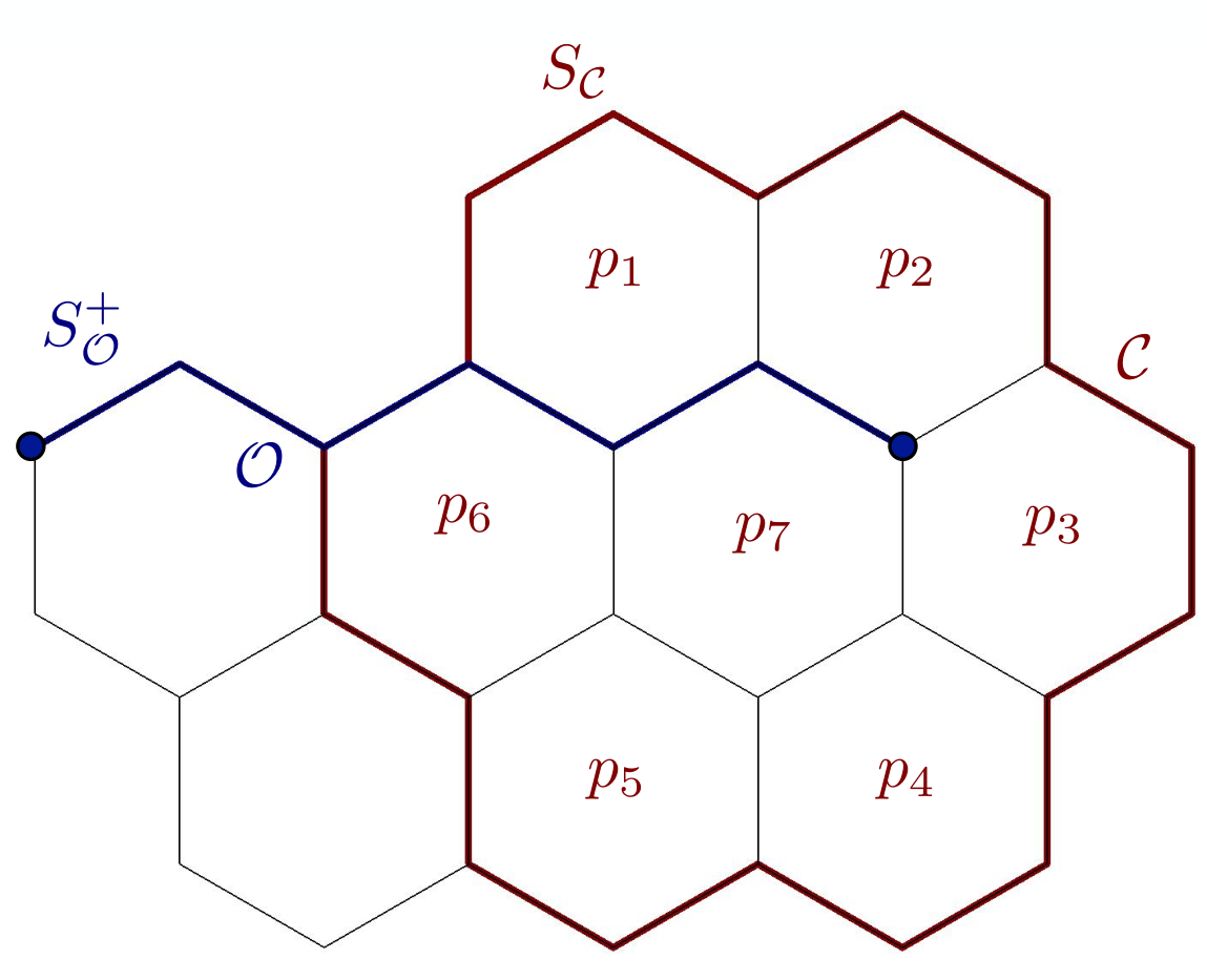
Refer to caption
Figure 13: A closed string, S𝒞S_{\mathcal{C}}, and a positive-chirality open string, S𝒪+S^{+}_{\mathcal{O}}, where paths 𝒪\mathcal{O} and 𝒞\mathcal{C} cross once. α→𝒞\vec{\alpha}^{\mathcal{C}} can be written in this particular example as α→𝒞=α→p1⊕⋯⊕α→p6\vec{\alpha}^{\mathcal{C}}=\vec{\alpha}^{p_{1}}\oplus\dots\oplus\vec{\alpha}^{p_{6}}, restricted to Conn(𝒞\mathcal{C}) . The multiplication of plaquettes inside 𝒞\mathcal{C}, i.e., Bp1​…​Bp7B_{p_{1}}...B_{p_{7}} is a negative-chirality string in Conn(𝒞\mathcal{C}).

C.3.1 Closed-string operators

If we consider now a closed path, 𝒞\mathcal{C}, and we use Algorithm 1 to find a closed-string operator, we will not find in general a positive-chirality nor a negative-chirality string, but some mixing of both. Physically, this is caused by the fact that for a closed string there is no difference in the pattern of plaquette violations between positive- and negative-chirality strings, since there are no endpoints. From Eq. (92) we can see that starting from a positive-chirality string, S𝒞+S^{+}_{\mathcal{C}}, it is possible to add SzS^{z} operators forming a loop which cannot be expressed as the product of vertex operators (which we call a non trivial loop in the remainder of the section) to the linear superposition. Once this is done, the resulting operator, S~𝒞\tilde{S}_{\mathcal{C}}, does not have a well-defined chirality. Remember, that for an open string, we may obtain the negative-chirality string by multiplying it by an open string SzS^{z}, violating the plaquettes at the endpoints. For closed strings we may proceed analogously to obtain the opposite chirality by multiplying by a non-trivial closed string S𝒞′zS^{z}_{\mathcal{C^{\prime}}}. Since we are multiplying S𝒞+S^{+}_{\mathcal{C}} by a linear combination of trivial and non-trivial loops of SzS^{z}, the chirality of S~𝒞\tilde{S}_{\mathcal{C}} is no longer positive nor negative. Thus, we drop the ‘++’ superscript in S~𝒞\tilde{S}_{\mathcal{C}}.

The mixing of chiralities becomes apparent when computing the commutator between a closed string, S𝒞S_{\mathcal{C}}, and a positive-chirality open string, S𝒪+S^{+}_{\mathcal{O}}, where paths 𝒞\mathcal{C} and 𝒪\mathcal{O} cross once (see Fig. 13):

ℛ𝒪,𝒞=⟨i→|[S𝒪+,S𝒞]|i→⟩=F𝒪​(i→⊕α→𝒞)​F𝒞​(i→)F𝒪​(i→)​F𝒞​(i→⊕α→𝒪),\mathcal{R_{O,C}}=\langle\vec{i}\;|\left[S^{+}_{\mathcal{O}},S_{\mathcal{C}}\right]|\vec{i}\;\rangle=\frac{F_{\mathcal{O}}\left(\vec{i}\oplus\vec{\alpha}^{\mathcal{C}}\right)F_{\mathcal{C}}\left(\vec{i}\;\right)}{F_{\mathcal{O}}\left(\vec{i}\;\right)F_{\mathcal{C}}\left(\vec{i}\oplus\vec{\alpha}^{\mathcal{O}}\right)}, (93)

where here [⋅,⋅][\cdot\;,\cdot] is the commutator in the group sense, i.e., [g,h]=g−1​h−1​g​h[g,h]=g^{-1}h^{-1}gh. In this case, notice that on Conn​(𝒞)\textnormal{Conn}(\mathcal{C}), the configurations i→\vec{i} and i→⊕α→𝒪\vec{i}\oplus\vec{\alpha}^{\mathcal{O}} do not belong to the same class. Using Eq. (91), it is thus clear that ℛ𝒪,𝒞\mathcal{R}_{\mathcal{O},\mathcal{C}} can be modified by selecting different phases to initialize F𝒞F_{\mathcal{C}} in Algorithm 1.

References