Near-critical percolation with heavy-tailed impurities,
forest fires and frozen percolation

We now describe in more detail the processes studied in, or relevant for, this paper. First, for the study of forest fire models, it appears to be very convenient to compare (couple) them with the classical percolation model, introduced by Broadbent and Hammersley [6] in 1957. More precisely, we consider Bernoulli site percolation with parameter $p\in[0,1]$ on a connected, countably infinite, graph $G=(V,E)$. In this model, each vertex $v\in V$ is occupied (or open, denoted by $1$), with probability $p$, and vacant (or closed, denoted by $0$), with probability $1-p$, independently of the other vertices. There is a critical value $p_{c}=p_{c}^{\textrm{site}}(G)\in[0,1]$ for the parameter $p$, below which (almost surely) all occupied clusters are finite, and above which there may be an infinite occupied cluster. This model (and variations, such as bond percolation) has been widely studied, especially on “nice” planar lattices like the square and the triangular lattices, and on the hypercubic lattices $\mathbb{Z}^{d}$, $d\geq 3$, with nearest-neighbor edges (the vertices of this lattice are the points with integer coordinates, and two such points $v$, $v^{\prime}$ are connected by an edge iff they differ along exactly one coordinate, by $\pm 1$).

The following model, which we will call the $N$-volume-frozen percolation model, or, sometimes, simply parameter-$N$ model, was studied in [38, 37], motivated by work by Aldous [1] (who in turn was inspired by phenomena concerning sol-gel transitions [32]). It has a (typically very large) parameter $N\geq 1$, and it is defined in terms of i.i.d. random variables $(\tau_{v})_{v\in V}$ uniformly distributed on $[0,1]$. Each vertex $v$ is vacant at time $0$, and becomes occupied at time $\tau_{v}$ unless some neighbor of $v$ already belongs to an occupied cluster with size (i.e. number of vertices) at least $N$ (in which case $v$ remains vacant). In other words, a cluster stops growing as soon as it has size $\geq N$: such a large cluster, together with its boundary, is said to be frozen, or “giant”.

What can we say about the probability that a given vertex eventually (i.e. at time $1$) belongs to a giant cluster? Of course, this is a function of $N$, and we are interested in what happens as $N\to\infty$. Does the above-mentioned probability go to $0$? Or is it bounded away from $0$? What is, typically, the final size (at time $1$) of the cluster of a given vertex? Of course, it cannot be larger than $d(N-1)+1$, where $d$ is the maximal degree of the graph, but is it typically smaller than $N$, and even of smaller order than $N$?

In the case where the graph is a binary tree, it was shown in [36] (by extending ideas from [1]) that with high probability as $N\to\infty$, the final cluster of a given vertex is either giant (i.e. has size $\geq N$) or “microscopic” (of order $1$). For the square lattice (and other “nice” planar lattices), it was shown in [38] that there is a sequence of functions ($\sqrt{N}\asymp$) $f_{1}(N)\ll f_{2}(N)\ll\ldots$ called exceptional scales such that the following holds: for each $i$, for the model in the box with side length $f_{i}(N)$, the probability that $0$ is eventually in a giant cluster is bounded away from $0$ as $N\to\infty$; however, for every function $f(N)$ with $f_{i}(N)\ll f(N)\ll f_{i+1}(N)$, the above-mentioned probability goes to $0$ as $N\to\infty$. In [37], it was shown (in the particular case of the triangular lattice) that this probability also tends to $0$ if $f(N)\gg f_{i}(N)$ for every $i\geq 1$, as well as for the process on the entire lattice.

As suggested above, the $N$-volume-frozen percolation model above can be interpreted as a simple model for gelation (sol-gel transition). It could (but see remarks below) also be interpreted as a model of forest fires (or epidemics) without recovery, where the ignitions (infections) are very rare ($N$ being very large), but once an ignition takes place, the fire spreads very fast, in effect wiping out instantaneously the entire occupied cluster. Initially, at each vertex there is one seed; once this seed has become a plant and this plant is burnt by fire, no other plant will grow at its location, and neither at neighboring locations. The role of the parameter $N$, i.e. that a cluster with size $\leq N$ cannot burn, is not very realistic for this interpretation: it makes the dynamic quite rigid. Also, the rule that nothing can grow any more on the sites along the external boundary of a burnt cluster of plants looks a bit artificial.

More realistic, as a model of forest fires without recovery, is the following, where time is now indexed by $[0,+\infty)$, and which has a (typically very small) parameter $\zeta>0$. Again, at time $0$, all vertices are vacant (or, better, contain a seed). Independently of each other, they become occupied (the seeds become plants) at rate $1$. Each occupied vertex (plant) is ignited at rate $\zeta$, in which case its entire occupied cluster is instantaneously burnt (and remains so). Note that in this process, there are three possible states for a vertex: $0$ (vacant, or “seed”: initially, all vertices are in this state), $1$ (occupied, or “plant”), and $-1$ (burnt). We will denote this process by the earlier-mentioned abbreviation FFWoR. It is clear from the description above that, for each $\zeta>0$, the probability that a given vertex is eventually in state $-1$ (i.e. burnt) is equal to $1$. The resulting configuration is depicted in Figure 1.1.

Analogs of (some of) the earlier questions are the following. Does, for each $t>0$, the probability that a given vertex burns before time $t$ go to $0$ as $\zeta\searrow 0$? Or are there values of $t$ for which this probability is bounded away from $0$ as $\zeta\searrow 0$? At first sight, one might expect that this model can be analyzed in the same way as the “parameter-$N$ model”, with (roughly) $N$ replaced by $\frac{1}{\zeta}$. Apart from the fact that this replacement is too naive, the arguments become considerably more complicated, due to quite delicate problems concerning what we call “near-critical percolation with impurities”, as we heuristically indicate now.

We will compare the parameter-$N$ model in a box with side length $f(N)$ with the FFWoR model with parameter $\zeta$ in a box with side length $g(\zeta)$. The heuristic arguments (made rigorous in [38]) for the parameter-$N$ model on the square lattice are roughly as follows. If $f(N)=C\sqrt{N}$ with $C>1$, then, clearly (since the total number of vertices is $>N$) at least one burning / freezing event will take place. Hence, a positive fraction ($\geq\frac{1}{C^{2}}$) of the vertices will freeze, which suggests (and this can be quite easily proved) that the probability that $0$ eventually freezes / burns is bounded away from $0$ (in fact, has limit $\frac{1}{C^{2}}$) as $N\to\infty$. Now, we try to find a function $f(N)\gg\sqrt{N}$ where this also holds, i.e. where the probability that $0$ burns / freezes is bounded away from $0$ as $N\to\infty$. To do this, let $\tau$ denote the first time that a giant cluster arises (recall that the time line in this model is the interval $[0,1]$). The biggest cluster at time $\tau$ has size roughly $\theta(\tau)f(N)^{2}$, where $\theta(\tau)$ is the probability (for Bernoulli site percolation on the whole lattice) that $0$ lies in an infinite occupied cluster at time $\tau$. We thus want

The freezing of this cluster disconnects the box into “islands” of diameter roughly of order $L(\tau)$ (the characteristic length for percolation with parameter $\tau$: see Section 2 for precise definitions of this and other notions). So if $\tau$ is such that $L(\tau)$ is of order $\sqrt{N}$, then $0$ will (after this freezing event) typically be in the interior of an island with diameter of order $\sqrt{N}$, and hence be in a similar situation as the previous case (i.e. the case where the box has side length $C\sqrt{N}$), so that the probability that $0$ freezes is bounded away from $0$. So we may choose $f(N)$ such that besides (1.1), also the following equation holds:

A celebrated and classical result by Kesten [18] says that $\theta(\tau)\asymp\pi_{1}(L(\tau))$, where $\pi_{1}(.)$ is the one-arm probability at $p_{c}$ (see (2.1) below). Combining (1.1) and (1.2) with this result gives $\pi_{1}(\sqrt{N})f(N)^{2}\asymp N$, hence

As a conclusion, if $f(N)$ is indeed of this order, then, for the parameter-$N$ model in a box with side length $f(N)$, the probability that $0$ freezes is bounded away from $0$ as $N\to\infty$. We say that $\sqrt{N}$ is the first exceptional scale, and (1.3) above is the second. Iterating this procedure produces a sequence of exceptional scales.

We now turn to the FFWoR model with parameter $\zeta>0$, and we will see that already the “construction” of the second exceptional scale involves new and delicate technical difficulties. First of all, similarly as in the parameter-$N$ model, it is not hard to see that for the process in a box with side length $\asymp\frac{1}{\sqrt{\zeta}}$, for each $t>t_{c}$, the probability that $0$ burns before time $t$ is bounded away from $0$ as $\zeta\searrow 0$ (here, time $t$ is related to the percolation parameter $p$ by $p=1-e^{-t}$; in particular, $p_{c}=1-e^{-t_{c}}$). The heuristic argument to find the next scale (call it $g(\zeta)$ for the moment) for which this happens is now as follows. Let $\tau$ be the first time that a big burning takes place, after which $0$ is separated from the boundary of the box. Analogously to the beginning of the argument for the parameter-$N$ model, the size of the biggest cluster at time $\tau>t_{c}$ is

At time $t_{c}$ it is much smaller, but at time $\frac{t_{c}+\tau}{2}$ it has already a size of order (1.4). So, to have a reasonable chance that the cluster burns “near” time $\tau$, we need

We apply again the earlier-mentioned relation by Kesten, which in the current notation is

as well as the following relation, also established by Kesten:

($\pi_{4}(.)$ is the probability at $p_{c}$ of observing four arms with alternating types from a given vertex, see (2.1)). Combining (1.5), (1.6) and (1.7) gives

Analogously as for the parameter-$N$ case, we want to take $g(\zeta)$ such that $L(\tau)\asymp\frac{1}{\sqrt{\zeta}}$ (so that after the burning, $0$ finds itself roughly in the same situation as before, i.e. the probability that $0$ burns before time $t$ does not vanish as $\zeta\searrow 0$). Plugging this requirement into (1.8), we get, as an analog of (1.3),

(and the next exceptional scales can be derived in a similar way).

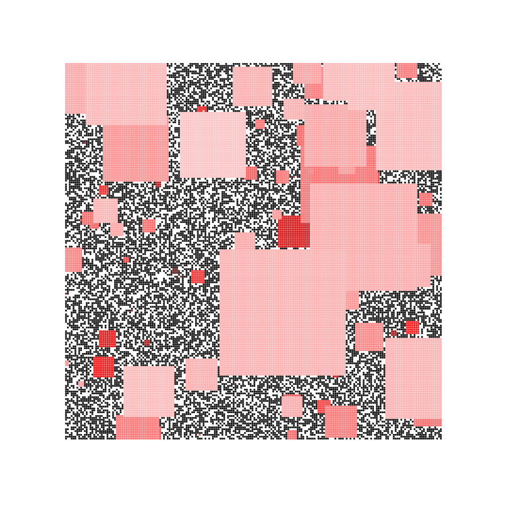
Note that the heuristics (and the formula: (1.9) involves not only $\pi_{1}$, but also $\pi_{4}$) for the FFWoR process is more “tricky” than that for the parameter-$N$ model. Moreover, there is a much more serious complication. Although the reasoning leading to (1.9) might look sound, there is a delicate issue which was “swept under the rug” and which has no analog in the parameter-$N$ model. Indeed, we ignored the smaller burnings which took place already before time $\tau$ and created “impurities” in the lattice (see Figure 1.2, produced by using the same realizations of the birth and the ignition processes as for Figure 1.1). For instance, the estimate (1.4) comes from ordinary percolation, but how do we know that in a model with impurities, this formula is still (more or less) correct? In fact, as we will see, the impurities are far from microscopic: we can consider them as “heavy-tailed”, and we have to understand their cumulative effect. This effect turns out to be much more complicated (and interesting) than we anticipated in the short, speculative, last section (Section 8) of [37].

We will present and study a quite general form of near-critical percolation with impurities, which happens to be crucial for a thorough analysis of the behavior of forest fire processes near (and beyond) the critical time, and in particular for handling the delicate issue mentioned above. Roughly speaking, we have to show that, for a certain class of “impurities”, the “global” connectivity properties of the percolation model are not (too) much worse than in the model without impurities (i.e. ordinary percolation). Figure 1.3 gives an illustration of the type of environments that we have to analyze.

The models of impurities that we are led to study are parametrized by a positive integer denoted by $m$, and they can be described as follows. Each vertex $v\in V$, independently of the other vertices, is the center of an impurity (a square box with a random side length) with a probability that we denote by $\pi^{(m)}$. If there is an impurity centered at $v$, the probability that it has a side length $\geq r$ is written as $\rho^{(m)}([r,+\infty))$ (for all $r\geq 0$). After removing all the impurities from the lattice, we perform Bernoulli percolation with parameter $p$ on the remaining graph.

Let us describe our choice of $\pi^{(m)}$ and $\rho^{(m)}$ more precisely. Let $c_{1},c_{2},c_{3}>0$ be constants, as well as $\alpha$ and $\beta$. Suppose that $\rho^{(m)}$ and $\pi^{(m)}$ are of the form

We then establish two kinds of results (which, so far, we can only prove for the triangular lattice, see Remark 2.1 below).

• 1.

  Stability properties for percolation with impurities. Results of the first kind say that the resulting percolation model mentioned above (i.e. Bernoulli percolation with parameter $p$, on the graph obtained by removing impurities) satisfies, under certain conditions, connectivity properties comparable to these of the pure percolation model. In particular, under some hypotheses on the values of $\alpha$ and $\beta$, and on the relation between $m$ and $L(p)$, the four-arm probabilities remain comparable (Theorem 4.1). We then use this to show that also one-arm probabilities, certain box-crossing probabilities, and, finally, the size of the largest cluster in a big box, remain comparable (see Propositions 5.1, 5.2, and 5.5).

• 2.

  Exceptional scales for forest fires with Poisson ignitions. These results are then used to derive the second kind of results, involving applications to the model of forest fires without recovery. In particular, these results give a rigorous verification of the existence of exceptional scales mentioned (and heuristically derived) in Section 1.2. This is done in Section 6 (where the relation with the general model with impurities is proved), and Section 7 (see Theorems 7.1 and 7.2).

The four-arm stability result (Theorem 4.1) turns out to be rather subtle. Indeed, we have to understand the effect of (possibly “mesoscopic”) impurities on “pivotal” events, which relies on a delicate balance between “helping” vacant arms with the impurities, but “hindering” occupied arms. Our proof uses the inequality $\alpha_{2}\geq\alpha_{4}+1$ between the two- and four-arm exponents for critical percolation, which can be checked (it is even an equality) from the actual values of these exponents. See Remark 4.2 and Section 4.3 for more background and details.

We comment a bit further on the percolation process with impurities, still assuming that $\rho^{(m)}$ and $\pi^{(m)}$ are of the form (1.10). Different behaviors arise according to the values of $\alpha$ and $\beta$, and we obtain the “phase diagram” depicted in Figure 1.4. After the present section, we will focus on Domain I, i.e. $\alpha\in\big(\frac{3}{4},2\big)$ and $\beta>\alpha$, which contains the relevant values for forest fires (this is Assumption 2 in Section 3.1): typically, $\alpha=\frac{55}{48}+\upsilon$ and $\beta=\alpha+\upsilon^{\prime}$, for some arbitrarily small $\upsilon,\upsilon^{\prime}>0$. We want to emphasize that the somewhat informal discussion in this section is mostly about other domains, rather than the one we concentrate on, and it is not required for the understanding of the rest of the paper.

First, note that as a special case, our framework contains classical near-critical percolation, studied in [18, 7, 26, 11]. Indeed, near-critical percolation with parameter $p<p_{c}$ can be constructed from the critical regime by performing single-site updates, i.e. letting the sites independently switch from occupied to vacant. It is obtained by taking $\rho^{(m)}=\delta_{0}$ (i.e. the Dirac mass at $0$, so that only impurities of radius $0$ are created) and $\pi^{(m)}\asymp\frac{1}{m^{2}\pi_{4}(m)}=m^{-\frac{1}{\nu}+o(1)}$, where $\nu=\frac{4}{3}$ is the critical exponent associated with $L$. This means that if we start from the critical regime and update the sites with a probability $\pi^{(m)}\asymp m^{-\beta}$, the resulting configuration is subcritical for $\beta<\frac{1}{\nu}=\frac{3}{4}$, and it stays near-critical for $\beta>\frac{1}{\nu}$.

We now briefly discuss the various domains in Figure 1.4. Observe that a short computation (similar to the one in Lemma 3.2 below) shows that the “density” of impurities, i.e. the probability for each vertex to be contained in at least one impurity, is of order $m^{\alpha_{+}-\beta}$.

• •

  Domain I: As mentioned in the previous section, we show that under appropriate hypotheses, percolation in the complement of the impurities stays comparable, in terms of connectedness, to ordinary percolation near criticality. We want to highlight that this behavior holds even when $\beta$ is very close to $\alpha$, which means that the exponent $\alpha-\beta$ for the density of impurities can be made arbitrarily close to $0$. This stands in contrast with the usual case of single-site updates, where this density has to stay below $m^{-\frac{3}{4}+o(1)}$. Roughly speaking, the behavior exhibited in Domain I comes from the particular way in which updates of sites are “arranged” spatially. Since they are grouped into balls, each of them has individually less effect. It emerges from explicit computations that the contribution of pivotal impurities is mainly produced by large impurities, with a radius of order $m$.

• •

  Domain II: Similar properties as in Domain I hold in this case, which is essentially covered by our proofs (see Section 4.2.4 below). However, the phenomenology in this domain is rather different since the main contribution of pivotal impurities is produced by microscopic impurities. Hence, the fact that the percolation configuration stays near-critical comes essentially from the same reasons as for single-site updates (this classical case corresponds to $\alpha=-\infty$ formally). Furthermore, for a given $\alpha<\frac{3}{4}$, the exponent $\alpha_{+}-\beta$ in the density of impurities stays smaller than $\alpha_{+}-\frac{3}{4}$, and so cannot be made arbitrarily close to $0$, contrary to Domain I.

• •

  Domain III: In this case, the configuration with impurities is clearly dominated by a configuration of Bernoulli percolation, obtained by using the same $\pi^{(m)}$, but with single-site updates (i.e. $\rho^{(m)}=\delta_{0}$). We know that in this case, the resulting configuration is subcritical for $\beta<\frac{3}{4}$.

• •

  Domain IV: When $\alpha>\beta$, the process is completely “degenerate”. For example, it is easy to see that for all $K>0$, with high probability (as $m\to\infty$), there exists an impurity centered on some $v\in B_{Km}$ that covers entirely $B_{Km}$.

We conclude this discussion by mentioning some works with a somewhat similar flavor, although the techniques and questions that we are studying in this paper are quite different in nature. Percolation on fractal-like graphs has been studied in e.g. [27, 20, 28, 29, 13, 15] (see also the discussion in Section 2.1 of [24]). There is also an extensive literature about a random walk / Brownian motion among randomly distributed obstacles: see for example the classical reference [33], the recent review [2], and the references therein.

Section 2 contains preliminaries about usual Bernoulli percolation. We first set notations, and then we collect classical results on the behavior of two-dimensional percolation through its phase transition, i.e. at and near its critical point.

In Sections 3 to 5, we analyze the percolation process with heavy-tailed impurities. We introduce it and present some of its properties in Section 3. Section 4 is devoted to stating and proving a stability result for four-arm events in the near-critical regime. This property is instrumental to derive further stability results, which we do in Section 5, culminating with a volume estimate for the largest connected component in a box.

We then make the connection with forest fire processes in Section 6: we introduce the exceptional scales $(m_{k}(\zeta))_{k\geq 1}$, and we collect some of their properties. We also explain how forest fires can be coupled to the process with impurities. In Section 7, we present some applications of the results developed earlier: we show that the scales $m_{k}$ are indeed exceptional for forest fire processes without recovery. Finally, in Section 8, we briefly discuss forest fire processes with recovery.

In the present paper, we work with the triangular lattice $\mathbb{T}=(V,E)$, with vertex set

and edge set $E:=\{\{v,v^{\prime}\}\>:\>v,v^{\prime}\in V\text{ with }|v-v^{\prime}|=1\}$ (using the standard identification $\mathbb{R}^{2}\simeq\mathbb{C}$). Two vertices $v,v^{\prime}\in V$ are said to be neighbors if they are connected by an edge, and we denote it by $v\sim v^{\prime}$. From now on, we always use the $L^{\infty}$ norm $\|.\|=\|.\|_{\infty}$. The inner (resp. outer) boundary of a subset $A\subseteq V$ is defined as $\partial^{\textrm{in}}A:=\{v\in A\>:\>v\sim v^{\prime}$ for some $v^{\prime}\in A^{c}\}$ (resp. $\partial^{\textrm{out}}A:=\partial^{\textrm{in}}(A^{c})$), and its volume, denoted by $|A|$, is simply the number of vertices that it contains.

Recall that Bernoulli site percolation on $\mathbb{T}$ with parameter $p\in[0,1]$ is obtained by declaring each vertex $v\in V$ either occupied or vacant, with respective probabilities $p$ and $1-p$, independently of the other vertices. We denote by $\mathbb{P}_{p}$ the corresponding product probability measure on configurations of sites $(\omega_{v})_{v\in V}\in\{0,1\}^{V}=:\Omega$.

A path of length $k$ ($k\geq 1$) is a sequence of vertices $v_{0}\sim v_{1}\sim\ldots\sim v_{k}$. Two vertices $v,v^{\prime}\in V$ are connected (denoted by $v\leftrightarrow v^{\prime}$) if there exists a path of length $k$ from $v$ to $v^{\prime}$, for some $k\geq 1$, containing only occupied sites (in particular, $v$ and $v^{\prime}$ have to be occupied). More generally, two subsets $A,A^{\prime}\subseteq V$ are connected if there exist $v\in A$ and $v^{\prime}\in A^{\prime}$ such that $v\leftrightarrow v^{\prime}$, which we denote by $A\leftrightarrow A^{\prime}$. Occupied vertices can be grouped into maximal connected components, or clusters. For a vertex $v\in V$, we denote by $\mathcal{C}(v)$ the occupied cluster of $v$, setting $\mathcal{C}(v)=\emptyset$ when $v$ is vacant. We write $v\leftrightarrow\infty$ for the event that $|\mathcal{C}(v)|=\infty$, i.e. $v$ lies in an infinite occupied cluster, and we introduce $\theta(p):=\mathbb{P}_{p}(0\leftrightarrow\infty)$. Site percolation on $\mathbb{T}$ displays a phase transition at the percolation threshold $p_{c}=p_{c}^{\textrm{site}}(\mathbb{T})$, and it is now a classical result [16] that $p_{c}=\frac{1}{2}$. Moreover, it is also known that $\theta(p_{c})=0$. Hence, for each $p\leq p_{c}=\frac{1}{2}$, there is almost surely no infinite cluster, while for $p>\frac{1}{2}$, there is almost surely a unique such cluster. The reader can consult the classical references [17, 12] for more background on percolation theory.

For a rectangle of the form $R=[x_{1},x_{2}]\times[y_{1},y_{2}]$ ($x_{1}<x_{2}$, $y_{1}<y_{2}$), an occupied path in $R$ “connecting the left and right (resp. top and bottom) sides” is called a horizontal (resp. vertical) crossing. Here, we use quotation marks because $R$ does not exactly “fit” the triangular lattice $\mathbb{T}$, so the definition needs to be made more accurate: this can be done easily, see for instance Definition 1 in Section 3.3 of [17] (the same remark applies to arm events, defined below). The event that such a crossing exists is denoted by $\mathcal{C}_{H}(R)$ (resp. $\mathcal{C}_{V}(R)$). We also write $\mathcal{C}_{H}^{*}(R)$ and $\mathcal{C}_{V}^{*}(R)$ for the corresponding events with paths of vacant vertices.

Let $B_{n}:=[-n,n]^{2}$ be the ball of radius $n\geq 0$ around $0$ for $\|.\|_{\infty}$. For $0\leq n_{1}<n_{2}$, we denote by $A_{n_{1},n_{2}}:=B_{n_{2}}\setminus B_{n_{1}}$ the annulus with radii $n_{1}$ and $n_{2}$ centered at $0$. For $z\in\mathbb{C}$, we write $B_{n}(z):=z+B_{n}$, and $A_{n_{1},n_{2}}(z):=z+A_{n_{1},n_{2}}$. Finally, we denote $A_{n_{1},\infty}(z):=(B_{n_{1}}(z))^{c}$. For an annulus $A=A_{n_{1},n_{2}}(z)$ ($0\leq n_{1}<n_{2}<\infty$, $z\in\mathbb{C}$), we denote by $\mathcal{O}(A)$ (resp. $\mathcal{O}^{*}(A)$) the existence of an occupied (resp. vacant) circuit in $A$. For $k\geq 1$ and $\sigma\in\mathfrak{S}_{k}:=\{o,v\}^{k}$ (where $o$ and $v$ stand for “occupied” and “vacant”, resp.), we introduce the arm event $\mathcal{A}_{\sigma}(A)$ that there exist $k$ disjoint paths $(\gamma_{i})_{1\leq i\leq k}$ in $A$, in counter-clockwise order, each with type prescribed by $\sigma_{i}$ (i.e. occupied or vacant path) and connecting $\partial^{\textrm{out}}B_{n_{1}}(z)$ to $\partial^{\textrm{in}}B_{n_{2}}(z)$. We use the notation

and we write $\pi_{\sigma}(n):=\pi_{\sigma}(1,n)$. For $k\geq 1$, we use the shorthand notations $\mathcal{A}_{k}$ and $\pi_{k}$ in the particular case when $\sigma=(ovo\ldots)\in\mathfrak{S}_{k}$ is alternating.

The usual characteristic length $L$ is defined by:

and $L(p)=L(1-p)$ for $p>p_{c}$. It follows from the Russo-Seymour-Welsh (RSW) bounds that at $p=p_{c}$, the probability in the right-hand side of (2.2) is $>0.001$ for all $n\geq 1$, so $L(p)\to\infty$ as $p\to p_{c}$, and we define $L(p_{c}):=\infty$. In the present paper, we consider a regularized version $\tilde{L}$, defined as follows. First, we set $\tilde{L}(p)=L(p)$ at each point of discontinuity $p\in(0,p_{c})\cup(p_{c},1)$ of $L$, $L(0)=L(1)=0$, and then we extend linearly $\tilde{L}$ to $[0,1]\setminus\{p_{c}\}$. The function $\tilde{L}$ has the additional property of being continuous and strictly increasing (resp. strictly decreasing) on $[0,p_{c})$ (resp. $(p_{c},1]$). In particular, it is a bijection from $[0,p_{c})$ (resp. $(p_{c},1]$) to $[0,\infty)$. In the following, we simply write $L$ instead of $\tilde{L}$.

Throughout the paper, we make use of the following classical properties of Bernoulli percolation, at and near the critical point $p_{c}$.

1. (i)

   RSW-type bounds. For all $K\geq 1$, there exists a constant $\delta_{4}=\delta_{4}(K)>0$ such that: for all $p\in(0,1)$ and $n\leq KL(p)$,

   $$\mathbb{P}_{p}\big(\mathcal{C}_{H}([0,4n]\times[0,n])\big)\geq\delta_{4}\quad\text{and}\quad\mathbb{P}_{p}\big(\mathcal{C}_{H}^{*}([0,4n]\times[0,n])\big)\geq\delta_{4}.$$

   (2.3)

   Note that since $L(p_{c})=\infty$, the first inequality actually holds for all $p\geq p_{c}$ and $n\geq 1$.

2. (ii)

   Exponential decay property. There exist universal constants $C_{1},C_{2}>0$ such that: for all $p>p_{c}$ and $n\geq 1$,

   $$\mathbb{P}_{p}\big(\mathcal{C}_{H}([0,4n]\times[0,n])\big)\geq 1-C_{1}e^{-C_{2}\frac{n}{L(p)}}$$

   (2.4)

   (see Lemma 39 in [25]).

3. (iii)

   Extendability of arm events. For all $k\geq 1$ and $\sigma\in\mathfrak{S}_{k}$, there exists a constant $C>0$ (that depends on $\sigma$ only) such that: for all $0\leq n_{1}<n_{2}$,

   $$\pi_{\sigma}\Big(\frac{n_{1}}{2},n_{2}\Big),\>\pi_{\sigma}(n_{1},2n_{2})\geq C\pi_{\sigma}(n_{1},n_{2})$$

   (2.5)

   (see Proposition 16 in [25]).

4. (iv)

   Quasi-multiplicativity of arm events. For all $k\geq 1$ and $\sigma\in\mathfrak{S}_{k}$, there exist $C_{1},C_{2}>0$ (depending only on $\sigma$) such that: for all $0\leq n_{1}<n_{2}<n_{3}$,

   $$C_{1}\pi_{\sigma}(n_{1},n_{3})\leq\pi_{\sigma}(n_{1},n_{2})\pi_{\sigma}(n_{2},n_{3})\leq C_{2}\pi_{\sigma}(n_{1},n_{3})$$

   (2.6)

   (see Proposition 17 in [25]).

5. (v)

   Arm exponents at criticality. For all $k\geq 1$, and $\sigma\in\mathfrak{S}_{k}$, there exists $\alpha_{\sigma}>0$ such that

   $$\pi_{\sigma}(k,n)=n^{-\alpha_{\sigma}+o(1)}\quad\text{as $n\to\infty$.}$$

   (2.7)

   Moreover, the value of $\alpha_{\sigma}$ is known, except in the monochromatic case (for $k\geq 2$ arms of the same type).

   • •

     For $k=1$, $\alpha_{\sigma}=\frac{5}{48}$.

   • •

     For all $k\geq 2$, and $\sigma\in\mathfrak{S}_{k}$ containing both types, $\alpha_{\sigma}=\frac{k^{2}-1}{12}$.

   These arm exponents were derived in [23, 31], based on the conformal invariance property of critical percolation [30] and properties of the Schramm-Loewner Evolution (SLE) processes (with parameter $6$, here) [21, 22].

6. (vi)

   Upper bound on monochromatic arm events. For all $k\geq 2$, let $\sigma=(o\ldots o)\in\mathfrak{S}_{k}$ be the monochromatic sequence of length $k$. There exist $C_{k},\beta_{k}>0$ such that: for all $0\leq n_{1}<n_{2}$,

   $$\pi_{\sigma}(n_{1},n_{2})\leq C_{k}\bigg(\frac{n_{1}}{n_{2}}\bigg)^{\beta_{k}}\pi_{k}(n_{1},n_{2}).$$

   (2.8)

   This follows from the proof of Theorem 5 in [4] (see in particular Step 1).

7. (vii)

   Stability for arm events near criticality. For all $k\geq 1$, $\sigma\in\mathfrak{S}_{k}$, and $K\geq 1$, there exist constants $C_{1},C_{2}>0$ (depending on $\sigma$ and $K$) such that: for all $p\in(0,1)$, and all $0\leq n_{1}<n_{2}\leq KL(p)$,

   $$C_{1}\pi_{\sigma}(n_{1},n_{2})\leq\mathbb{P}_{p}\big(\mathcal{A}_{\sigma}(A_{n_{1},n_{2}})\big)\leq C_{2}\pi_{\sigma}(n_{1},n_{2})$$

   (2.9)

   (see Theorem 27 in [25]).

8. (viii)

   Asymptotic equivalences for $\theta$ and $L$. We have

   $$\theta(p)\asymp\pi_{1}(L(p))\quad\text{as $p\searrow p_{c}$}$$

   (2.10)

   (see Theorem 2 in [18], or (7.25) in [25]), and

   $$\big|p-p_{c}\big|L(p)^{2}\pi_{4}\big(L(p)\big)\asymp 1\quad\text{as $p\to p_{c}$}$$

   (2.11)

   (see (4.5) in [18], or Proposition 34 in [25]).

9. (ix)

   A-priori bounds on arm events. There exist universal constants $C_{i}>0$ ($1\leq i\leq 4$) and $\beta_{j}>0$ ($1\leq j\leq 3$) such that the following inequalities hold. For all $p\in(0,1)$ and $0\leq n_{1}<n_{2}\leq L(p)$,

   $$C_{1}\bigg(\frac{n_{1}}{n_{2}}\bigg)^{1/2}\leq\mathbb{P}_{p}\big(\mathcal{A}_{1}(A_{n_{1},n_{2}})\big)\leq C_{2}\bigg(\frac{n_{1}}{n_{2}}\bigg)^{\beta_{1}}$$

   (2.12)

   (the upper bound is an immediate consequence of (2.3), while the lower bound follows from the van den Berg-Kesten inequality), and

   $$C_{3}\bigg(\frac{n_{1}}{n_{2}}\bigg)^{2-\beta_{2}}\leq\mathbb{P}_{p}\big(\mathcal{A}_{4}(A_{n_{1},n_{2}})\big)\leq C_{4}\bigg(\frac{n_{1}}{n_{2}}\bigg)^{1+\beta_{3}}.$$

   (2.13)

   The left-hand inequality in (2.13) follows from the “universal” arm exponent for $\mathcal{A}_{5}$ which is equal to $2$ (see Theorem 24 (3) in [25]) together with (2.12), and the right-hand inequality follows from Corollary 2 in [18] (more precisely, the lower bound on the critical exponent $\nu$ associated with $L$) combined with (2.11).

10. (x)

    Volume estimates. Let $(n_{k})_{k\geq 1}$ be a sequence of integers, with $n_{k}\to\infty$ as $k\to\infty$, and $(p_{k})_{k\geq 1}$ satisfying $p_{c}<p_{k}<1$. If $L(p_{k})\ll n_{k}$ as $k\to\infty$, then

    $$\text{for all $\varepsilon>0$,}\quad\mathbb{P}_{p_{k}}\left(\frac{|\mathcal{C}^{\textrm{max}}_{B_{n_{k}}}|}{\theta(p_{k})|B_{n_{k}}|}\notin(1-\varepsilon,1+\varepsilon)\right)\mathrel{{\mathop{\longrightarrow}\limits}}0,$$

    (2.14)

    where we denote by $|\mathcal{C}^{\textrm{max}}_{B_{n_{k}}}|$ the volume of the largest occupied cluster in $B_{n_{k}}$ (see Theorem 3.2 in [5]).

The following geometric construction is used repeatedly in our proofs.

For the percolation configuration inside $B_{n}$, the event $\mathcal{N}_{p}(n,\kappa)$ implies the existence of a $p$-occupied connected set $\mathcal{N}$ such that all the connected components of its complement (so in particular, all the $p$-occupied and $p$-vacant connected components other than the cluster $\mathcal{C}_{\mathcal{N}}$ of $\mathcal{N}$ in $B_{n}$) have a diameter at most $4\kappa$. Such a set $\mathcal{N}$ is called net with mesh $\kappa$. Note also that $\mathcal{N}_{p}(n,\kappa)$ does not depend on the sites in $B_{\kappa}$.

Recall the following exponential upper bound for the probability of observing abnormally large clusters (see Lemma 4.4 in [37]).

We will also need a more uniform version of (2.7).

Recall the forest fire processes described in the Introduction. Intuitively, as $t$ approaches $t_{c}$, larger and larger clusters appear, thus creating larger and larger vacant regions when they burn. We have to understand the cumulative effect of these burnings on the connectivity of the percolation configuration: in principle, the “destroyed” areas could, at some point, be so large that they hinder the creation of new large connected components. We study the interplay between these competing effects by introducing a percolation process on a “randomly perforated” lattice. Roughly speaking, as we will see later, this process provides a good picture of the forest slightly before time $t_{c}$, in particular whether it is sufficiently connected for large-scale fires to occur.

In the following, we consider a lattice with “impurities”, that we call holes from now on. Let $\pi$ be a parameter in $[0,1]$, and $\rho$ a distribution on $[0,+\infty)$ that describes the radii of the holes. We put holes on $V$ in the following fashion. For each vertex $v\in V$, independently of the other vertices, we draw a radius $r_{v}$ distributed according to $\rho$, and we put a hole centered on $v$ with a probability $\pi$ (typically $\ll 1$): in this case, we remove from the lattice all the vertices in the hole $H_{v}:=B_{r_{v}}(v)$, i.e. within a distance $r_{v}$ (for the norm $\|.\|_{\infty}$) from $v$ (see Figure 3.1). If there is no hole centered on $v$, we set $H_{v}:=\emptyset$.

For technical reasons, we also need to allow $\pi$ to depend on $v$, i.e. we consider inhomogeneous $\pi=(\pi_{v})_{v\in V}$. Let $I_{v}$ be the indicator that there is a hole centered at $v$ (so that $I_{v}=1$ with probability $\pi_{v}$). We always assume that the random variables $(I_{v})_{v\in V}$ and $(r_{v})_{v\in V}$ are independent.

We obtain in this way a random subgraph of $\mathbb{T}$, and we are interested in its connectedness. In particular, we want to study independent site percolation with parameter $p\in[0,1]$ on this subgraph, i.e. on the complement of the holes. Note that a totally equivalent way of seeing it is by first considering an independent site percolation configuration on $\mathbb{T}$, and then partially “destroy” it with holes (we think of the vertices in the holes as simply being vacant): are the large-scale connectivity properties of the percolation configuration significantly affected by the holes? We obtain a probability measure on configurations of holes and percolation configurations on the complement of the holes, that we denote by $\overline{\mathbb{P}}_{p}^{\pi,\rho}$. Sometimes, we forget about the dependence on $\pi$ and $\rho$, when they are clear from the context, and we just write $\overline{\mathbb{P}}_{p}$. For events regarding only the configuration of holes, we use the notation $\overline{\mathbb{P}}^{\pi,\rho}$.

Of course, the macroscopic behavior of the $\overline{\mathbb{P}}_{p}^{\pi,\rho}$ process depends on the particular choice of $\pi$ and $\rho$, and we focus on the following setting where they depend on a parameter $m\to\infty$. We assume that $\rho^{(m)}$ is “heavy-tailed”, and that a uniform power-law upper bound on $\pi^{(m)}_{v}$ holds. More precisely:

We will be mostly interested in values of $p$ in near-critical windows around $p_{c}$ of the form $\{p\>:\>L(p)\geq\kappa m\}$, for fixed $\kappa>0$. As we explain in Section 6.4, the $\overline{\mathbb{P}}_{p}^{(m)}$ processes arise naturally in the study of forest fires, at times close to the critical time $t_{c}$. In this case, the truncation parameter $m$ (the typical radius of the largest holes) plays the role of a characteristic scale for the holes created by fires up to some time slightly before $t_{c}$.

As we mentioned in Section 1.4, the $\overline{\mathbb{P}}_{p}^{(m)}$ process behaves asymptotically (as $m\to\infty$) in very different ways according to the values of $\alpha<2$ and $\beta>0$. For applications to forest fires, the relevant values turn out to belong to Domain I of Figure 1.4. We thus focus on this domain, i.e. we assume the following in the remainder of the paper.

As we will see, the most interesting behavior arises precisely in this domain. We prove that for any such $\alpha$ and $\beta$, the holes do not have a significant effect on the connectedness of the lattice, in the following sense. As $m\to\infty$, for values $p\in(p_{c},1)$ satisfying $L(p)\asymp m$, percolation outside the holes stays “near-critical”: it is comparable to critical percolation up to scales of order $m$, and to supercritical percolation on larger scales (see Sections 4 and 5 for precise statements).

Recall that from now on (and until the end of Section 5), we consider a sequence of measures $\overline{\mathbb{P}}_{p}^{(m)}=\overline{\mathbb{P}}_{p}^{\pi^{(m)},\rho^{(m)}}$, where we assume that $\rho^{(m)}$ and $(\pi^{(m)}_{v})_{v\in V}$ satisfy (3.1) for some given $c_{1},c_{2},c_{3}\in(0,+\infty)$, and $(\alpha,\beta)$ as in (3.3), i.e. in Domain I. All the asymptotic results stated below for $m\to\infty$ are uniform in such $\rho^{(m)}$ and $(\pi^{(m)}_{v})_{v\in V}$, although we will not repeat it every time, for the sake of conciseness.

The following lemma turns out to be particularly handy, and we make repeated use of it in our proofs. For an annulus $A=A_{n_{1},n_{2}}(z)$ ($z\in\mathbb{C}$, $1\leq n_{1}<n_{2}$), we introduce the event that it is “crossed” by a hole, i.e.

Note that in this definition, we do not require the vertex $v$ to be in $A$: the crossing hole is allowed to be centered outside of $A$. Occasionally, we will use the straightforward generalization of (3.4) when instead of $B_{n_{1}}(z)$ and $B_{n_{2}}(z)$, we have rectangles $R$ and $R^{\prime}$ with $R\subseteq R^{\prime}$.

References

• [1] David J. Aldous. The percolation process on a tree where infinite clusters are frozen. Math. Proc. Cambridge Philos. Soc., 128(3):465–477, 2000.
• [2] Siva Athreya, Alexander Drewitz, and Rongfeng Sun. Random walk among mobile/immobile traps: a short review. Preprint arXiv:1703.06617, 2017.
• [3] Per Bak. How nature works: the science of self-organized criticality. Copernicus, New York, 1996.
• [4] Vincent Beffara and Pierre Nolin. On monochromatic arm exponents for 2D critical percolation. Ann. Probab., 39(4):1286–1304, 2011.
• [5] Christian Borgs, Jennifer T. Chayes, Harry Kesten, and Joel Spencer. The birth of the infinite cluster: finite-size scaling in percolation. Comm. Math. Phys., 224(1):153–204, 2001.
• [6] S. R. Broadbent and J. M. Hammersley. Percolation processes. I. Crystals and mazes. Proc. Cambridge Philos. Soc., 53:629–641, 1957.
• [7] Federico Camia, Luiz Renato G. Fontes, and Charles M. Newman. The scaling limit geometry of near-critical 2D percolation. J. Stat. Phys., 125(5-6):1159–1175, 2006.
• [8] Michael Damron, Artëm Sapozhnikov, and Bálint Vágvölgyi. Relations between invasion percolation and critical percolation in two dimensions. Ann. Probab., 37(6):2297–2331, 2009.
• [9] Barbara Drossel and Franz Schwabl. Self-organized critical forest-fire model. Phys. Rev. Lett., 69:1629–1632, 1992.
• [10] Maximilian Dürre. Existence of multi-dimensional infinite volume self-organized critical forest-fire models. Electron. J. Probab., 11:no. 21, 513–539, 2006.
• [11] Christophe Garban, Gábor Pete, and Oded Schramm. The scaling limits of near-critical and dynamical percolation. J. Eur. Math. Soc., 20(5):1195–1268, 2018.
• [12] Geoffrey Grimmett. Percolation, volume 321 of Grundlehren der Mathematischen Wissenschaften. Springer-Verlag, Berlin, second edition, 1999.
• [13] Yasunari Higuchi and Xian-Yuan Wu. Uniqueness of the critical probability for percolation in the two-dimensional Sierpiński carpet lattice. Kobe J. Math., 25(1-2):1–24, 2008.
• [14] Henrik J. Jensen. Self-organized criticality: emergent complex behavior in physical and biological systems, volume 10 of Cambridge Lecture Notes in Physics. Cambridge University Press, Cambridge, 1998.
• [15] Michael Keane and Masato Takei. A conditionally sure ergodic theorem with an application to percolation. Stochastic Process. Appl., 124(11):3651–3660, 2014.
• [16] Harry Kesten. The critical probability of bond percolation on the square lattice equals 1/2. Comm. Math. Phys., 74(1):41–59, 1980.
• [17] Harry Kesten. Percolation theory for mathematicians, volume 2 of Progress in Probability and Statistics. Birkhäuser, Boston, 1982.
• [18] Harry Kesten. Scaling relations for 22D-percolation. Comm. Math. Phys., 109(1):109–156, 1987.
• [19] Demeter Kiss, Ioan Manolescu, and Vladas Sidoravicius. Planar lattices do not recover from forest fires. Ann. Probab., 43(6):3216–3238, 2015.
• [20] Takashi Kumagai. Percolation on pre-Sierpinski carpets. In New trends in stochastic analysis (Charingworth, 1994), pages 288–304. World Sci. Publ., River Edge, NJ, 1997.
• [21] Gregory F. Lawler, Oded Schramm, and Wendelin Werner. Values of Brownian intersection exponents. I. Half-plane exponents. Acta Math., 187(2):237–273, 2001.
• [22] Gregory F. Lawler, Oded Schramm, and Wendelin Werner. Values of Brownian intersection exponents. II. Plane exponents. Acta Math., 187(2):275–308, 2001.
• [23] Gregory F. Lawler, Oded Schramm, and Wendelin Werner. One-arm exponent for critical 2D percolation. Electron. J. Probab., 7:no. 2, 13 pp., 2002.
• [24] Jason Miller, Scott Sheffield, and Wendelin Werner. CLE percolations. Forum Math. Pi, 5:e4, 102 pp., 2017.
• [25] Pierre Nolin. Near-critical percolation in two dimensions. Electron. J. Probab., 13:no. 55, 1562–1623, 2008.
• [26] Pierre Nolin and Wendelin Werner. Asymmetry of near-critical percolation interfaces. J. Amer. Math. Soc., 22(3):797–819, 2009.
• [27] Masato Shinoda. Percolation on the pre-Sierpiński gasket. Osaka J. Math., 33(2):533–554, 1996.
• [28] Masato Shinoda. Existence of phase transition of percolation on Sierpiński carpet lattices. J. Appl. Probab., 39(1):1–10, 2002.
• [29] Masato Shinoda. Non-existence of phase transition of oriented percolation on Sierpinski carpet lattices. Probab. Theory Related Fields, 125(3):447–456, 2003.
• [30] Stanislav Smirnov. Critical percolation in the plane: conformal invariance, Cardy’s formula, scaling limits. C. R. Acad. Sci. Paris Sér. I Math., 333(3):239–244, 2001.
• [31] Stanislav Smirnov and Wendelin Werner. Critical exponents for two-dimensional percolation. Math. Res. Lett., 8(5-6):729–744, 2001.
• [32] Walter H. Stockmayer. Theory of molecular size distribution and gel formation in branched-chain polymers. Journal of Chemical Physics, 11:45–55, 1943.
• [33] Alain-Sol Sznitman. Brownian motion, obstacles and random media. Springer Monographs in Mathematics. Springer-Verlag, Berlin, 1998.
• [34] Jacob van den Berg and Rachel Brouwer. Self-destructive percolation. Random Structures Algorithms, 24(4):480–501, 2004.
• [35] Jacob van den Berg and Rachel Brouwer. Self-organized forest-fires near the critical time. Comm. Math. Phys., 267(1):265–277, 2006.
• [36] Jacob van den Berg, Demeter Kiss, and Pierre Nolin. A percolation process on the binary tree where large finite clusters are frozen. Electron. Commun. Probab., 17(2):1–11, 2012.
• [37] Jacob van den Berg, Demeter Kiss, and Pierre Nolin. Two-dimensional volume-frozen percolation: deconcentration and prevalence of mesoscopic clusters. Ann. Sci. Éc. Norm. Supér. (4), 51(4):1017–1084, 2018.
• [38] Jacob van den Berg and Pierre Nolin. Two-dimensional volume-frozen percolation: exceptional scales. Ann. Appl. Probab., 27(1):91–108, 2017.
• [39] David Wilkinson and Jorge F. Willemsen. Invasion percolation: a new form of percolation theory. Journal of Physics A: Mathematical and General, 16:3365–3376, 1983.