A Unified Approach to Translate Classical Bandit Algorithms to the Structured Bandit Setting
Abstract
We consider a finite-armed structured bandit problem in which mean rewards of different arms are known functions of a common hidden parameter . Since we do not place any restrictions on these functions, the problem setting subsumes several previously studied frameworks that assume linear or invertible reward functions. We propose a novel approach to gradually estimate the hidden and use the estimate together with the mean reward functions to substantially reduce exploration of sub-optimal arms. This approach enables us to fundamentally generalize any classical bandit algorithm including UCB and Thompson Sampling to the structured bandit setting. We prove via regret analysis that our proposed UCB-C algorithm (structured bandit versions of UCB) pulls only a subset of the sub-optimal arms times while the other sub-optimal arms (referred to as non-competitive arms) are pulled times. As a result, in cases where all sub-optimal arms are non-competitive, which can happen in many practical scenarios, the proposed algorithm achieves bounded regret. We also conduct simulations on the Movielens recommendations dataset to demonstrate the improvement of the proposed algorithms over existing structured bandit algorithms.
1 Introduction
1.1 Overview
The Multi-armed bandit problem (Lai and Robbins 1985) (MAB) falls under the umbrella of sequential decision-making problems. It has numerous applications such as clinical trials (Villar et al. 2015), system testing (Tekin and Turgay 2017), scheduling in computing systems (Nino-Mora 2009), and web optimization (White 2012; Sen et al. 2017), to name a few. In the classical -armed bandit formulation, a player is presented with arms. At each time step , she decides to pull an arm and receives a random reward with unknown mean . The goal of the player is to maximize their expected cumulative reward (or equivalently, minimize expected cumulative regret) over time steps. In order to do so, the player must strike a balance between estimating the unknown rewards accurately by pulling all the arms (exploration) and always pulling the current best arm (exploitation). The seminal work of Lai and Robins (1985) proposed the Upper Confidence Bound (UCB) algorithm that balances the exploration-exploitation tradeoff in the MAB problem. Subsequently, several algorithms such as UCB1 (Auer et al. 2002), Thompson Sampling (TS) (Agrawal and Goyal 2012) and KL-UCB (Garivier and Cappé 2011) were proposed and analyzed for the classical MAB setting.
In this paper, we study a fundamental variant of classical multi-armed bandits called the structured multi-armed bandit problem, where mean rewards of the arms are functions of a hidden parameter . That is, the expected reward of arm is a known function of the parameter that lies in a (known) set . However, the true value of , denoted as , is unknown. The dependence of mean rewards on the common parameter introduces a structure in the MAB problem. For example, rewards observed from an arm may provide partial information about the mean rewards of other arms, making it possible to significantly lower the resulting cumulative regret as compared to the classical MAB setting.
Structured bandit models arise in many applications and have been studied by several authors with motivating applications including dynamic pricing (described in Atan et al. 2015), cellular coverage optimization (by Shen et al. 2018), drug dosage optimization (discussed in Wang et al. 2018) and system diagnosis; see Section 1.2 for an illustrative application of the structured MAB framework. In this paper, we consider a general version of the structured MAB framework that subsumes and generalizes several previously considered settings. More importantly, we propose a novel and unified approach that would allow extending any current or future MAB algorithm (UCB, TS, KL-UCB, etc.) to the structured setting; see Sections 1.3 and 3 for our main contributions and a comparison of our work with related literature.
1.2 An Illustrative Example

For illustration purposes, consider the example of movie recommendation, where a company would like to decide which movie(s) to recommend to each user with the goal of maximizing user engagement (e.g., in terms of click probability and time spent watching, etc.). In order to achieve this, the company needs to identify the most appealing movie for the user in an online manner and this is where multi-armed bandit algorithms can be helpful. However, classical MAB algorithms are typically based on the (implicit) assumption that rewards from different arms (i.e., different movies in this context) are independent of each other. This assumption is unlikely to hold in reality since the user choices corresponding to different movies are likely to be related to each other; e.g., the engagement corresponding to different movies may depend on the age/occupation/income/taste of the user.
To address this, contextual bandits (Li et al. 2010; Sen et al. 2018) have been proposed and studied widely for personalized recommendations. There, it is assumed that before making a choice (of which movie to recommend), a context feature of the user is observed; the context can include personal information of the user including age, occupation, income, or previous browsing information. Contextual bandit algorithms aim to learn the mapping from context information to the most appealing arm, and can prove useful in applications involving personalized recommendations (or, advertising). However in several use cases, observing contextual features leads to privacy concerns. In addition, the contextual features may not be visible for new users or users who are signed in anonymously to protect their identity.
The structured bandit setting considered in this paper (and by many others Atan et al. 2015; Shen et al. 2018; Wang et al. 2018) can be viewed as the same problem setting with contextual bandits with the following difference. Unlike contextual bandits, the context of the users are hidden in the structured setting, but in return it is assumed that the mappings from the contexts to mean rewards of arms are known a priori. It is anticipated that the mean reward mappings can be learned from paid surveys in which users participate with their consent. The proposed structured bandit framework’s goal is to use this information to provide the best recommendation to an anonymous user whose context vector is unknown; e.g., see Figure 1. Thus, our problem formulation is complementary to contextual bandits; in contextual bandits the context is known while the reward mappings are unknown, whereas in our setting is unknown and the mean rewards are known. A detailed problem formulation discussing the assumptions and extensions of this set-up is given in Section 2.
1.3 Main Contributions and Organization
We summarize the key contributions of the paper below. The upcoming sections will develop each of these in detail.
- 1.
General Setting Subsuming Previous Works: Structured bandits have been studied in the past (Atan et al. 2015; Wang et al. 2018; Mersereau et al. 2009; Filippi et al. 2010; Lattimore and Szepesvari 2016; Graves and Lai 1997) but with certain restrictions (e.g., being linear, invertible, etc.) on the mean reward mappings . We consider a general setting that puts no restrictions on the mean reward mappings. In fact, our setting subsumes recently studied models such as Global Bandits (Atan et al. 2015), Regional Bandits (Wang et al. 2018) and structured bandits with linear rewards (Mersereau et al. 2009); see Section 3 for a detailed comparison with previous works.
There are a couple of recent works (Lattimore and Munos 2014; Combes et al. 2017) that do consider a general structured bandit setting similar to our work – see Section 3 for details. Our approach differs from these in its flexibility to extend any classical bandit algorithm (UCB, Thompson sampling, etc.) to the structured bandit setting. In particular, using Thompson sampling (Thompson 1933; Agrawal and Goyal 2013b) as the underlying bandit algorithm yields a robust and empirically superior way (see Section 5.4) to minimize superfluous exploration. The UCB-S algorithm proposed in (Lattimore and Munos 2014) extends the UCB algorithm to structured setting. However, the approach presented in (Lattimore and Munos 2014) can not be extended to Thompson sampling or other classical bandit algorithms; in fact, this point was highlighted in (Lattimore and Munos 2014) as an open question for future work. In (Combes et al. 2017), there are several assumptions in the model that are not imposed here, including the assumption that the conditional reward distributions are known and reward mappings are continuous. In addition, the main focus of (Combes et al. 2017) is the parameter regime where regret scales logarithmically with time , while our approach demonstrates the possibility of achieving bounded regret.
- 2.
Extending any classical bandit algorithm to the structured bandit setting: We propose a novel and unified approach that would allow extending any classical or future MAB algorithm (that is developed for the non-structured setting) to the structured bandit framework given in Figure 2. Put differently, we propose a class of structured bandit algorithms referred to as Algorithm-C, where “Algorithm" can be any classical bandit algorithm including UCB, TS, KL-UCB, etc. A detailed description of the resulting algorithms, e.g., UCB-C, TS-C, etc., are given in Section 4 with their steps illustrated in Figure 3.
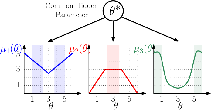
Figure 2: Structured bandit setup: mean rewards of different arms share a common hidden parameter. This example illustrates a 3-armed bandit problem with shaded regions indicating the values of for which the particular arm is optimal. - 3.
Unified regret analysis: A key benefit of our algorithms is that they pull a subset of the arms (referred to as the non-competitive arms) only times. Intuitively, an arm is non-competitive if it can be identified as sub-optimal with high probability using only the samples from the optimal arm . This is in contrast to classical MAB algorithms where all sub-optimal arms are pulled times, where is the total number of rounds. This is shown by analyzing the expected regret , which is the difference between the expected cumulative reward obtained by using the proposed algorithm and the expected cumulative reward of a genie policy that always pulls the optimal arm . In particular, we provide rigorous regret analysis for UCB-C as summarized in the theorem below, and describe how our proof technique can be extended to other classical MAB algorithms.
Theorem 1 (Expected Regret Scaling).
The expected regret of the UCB-C algorithm has the following scaling with respect to the number of rounds :
(1) where is the number of competitive arms (including the optimal arm ) and is the true value of the hidden parameter. The remaining arms are called non-competitive. An arm is said to be non-competitive if there exists an such that for all , where (more details in Section 5).
The exact regret upper bound with all the constants follows from 2 and 3 in Section 5. Recall that for the standard MAB setting (Lai and Robbins 1985), the regret upper bound is , where is the total number of arms. 1 reveals that with our algorithms only out of the sub-optimal arms are pulled times. The other arms are pulled only times.
- 4.
Reduction in the effective number of arms. For any given set of reward functions , the number of competitive arms depends on the unknown parameter ; see Figure 4 in Section 5 for an illustration of this fact. We show that can be much smaller than in many practical cases. This is because, the reward functions (particularly that corresponding to the optimal arm) can provide enough information about the hidden , which in turn can help infer the sub-optimality of several other arms. More specifically, this happens when the reward functions are not flat around , that is, the pre-image set of { is small. In the special case where the optimal arm is invertible or has a unique maximum at , and our algorithms can achieve regret.
- 5.
Evaluation on real-world datasets: In Section 5, we present extensive simulations comparing the regret of the proposed algorithm with previous methods such as GLM-UCB (Filippi et al. 2010) and UCB-S (Lattimore and Munos 2014). We also present simulation results for the case where the hidden parameter is a vector. In Section 7, we perform experiments on the Movielens dataset to demonstrate the applicability of the UCB-C and TS-C algorithms. Our experimental results show that both UCB-C and TS-C lead to significant improvement over the performance of existing bandit strategies. In particular, TS-C is shown to consistently outperform all other algorithms across a wide range of settings.
2 Problem Formulation
Consider a multi-armed bandit setting with the set of arms . At each round , the player pulls arm and observes a reward . The reward is a random variable with mean , where is a fixed, but unknown parameter which lies in a known set ; see Figure 2.
We denote the (unknown) true value of by . There are no restrictions on the set . Although we focus on scalar in this paper for brevity, the proposed algorithms and regret analysis can be generalized to the case where we have a hidden parameter vector . In Section 5, we present simulation results for the case of a parameter vector . The mean reward functions for can be arbitrary functions of with no linearity or continuity constraints imposed. While are known to the player, the conditional distribution of rewards, i.e., is not known.
We assume that the rewards are sub-Gaussian with variance proxy , i.e.,
, and is known to the player. Both assumptions are common in the multi-armed bandit literature (Bubeck et al. 2012; Jamieson and Nowak 2014; Atan et al. 2015; Lattimore and Munos 2014).
In particular, the sub-Gaussianity of rewards enables us to apply Hoeffding’s inequality, which is essential for the analysis of regret (defined below).
The objective of the player is to select arm in round so as to maximize her cumulative reward after rounds. If the player had known the hidden , then she would always pull arm that yields the highest mean reward at . We refer to as the optimal arm. Maximizing the cumulative reward is equivalent to minimizing the cumulative regret, which is defined as
where is the number of times arm is pulled in slots and is the sub-optimality gap of arm . Minimizing the cumulative regret is in turn equivalent to minimizing , the number of times each sub-optimal arm is pulled.
Remark 1 (Connection to classical Multi-armed Bandits).
The classical multi-armed bandit setting, which does not explicitly consider a structure among the mean rewards of different arms, is a special case of the proposed structured bandit framework. It corresponds to having a hidden parameter vector and the mean reward of each arm being . In fact, our proposed algorithm described in Section 4 reduces to standard UCB or Thompson sampling (Lai and Robbins 1985; Auer et al. 2002) in this special case.
The proposed structured bandit subsumes several previously considered models where the rewards are assumed to be linear (Mersereau et al. 2009; Lattimore and Szepesvari 2016), invertible and Hölder continuous (Atan et al. 2015; Wang et al. 2018), etc. See Section 3 for a detailed comparison with these works.
3 Related Work
Since we do not make any assumptions on the mean reward functions , our model subsumes several previously studied frameworks (Atan et al. 2015; Wang et al. 2018; Mersereau et al. 2009). The similarities and differences between our model and existing works are discussed below.
Structured bandits with linear rewards (Mersereau et al. 2009). In (Mersereau et al. 2009), the authors consider a similar model with a common hidden parameter , but the mean reward functions, are linear in . Under this assumption, they design a greedy policy that achieves bounded regret. Our formulation does not make linearity assumptions on the reward functions. In the special case when are linear, our proposed algorithm also achieves bounded regret.
Global and regional bandits. The papers (Atan et al. 2015; Wang et al. 2018) generalize this to invertible and Hölder-continuous reward functions. Instead of scalar , (Wang et al. 2018) considers common unknown parameters, that is, . Under these assumptions, (Atan et al. 2015; Wang et al. 2018) demonstrate that it is possible to achieve bounded regret through a greedy policy. In contrast, our work makes no invertibility or continuity assumptions on the reward functions . In the special case when are invertible, our proposed algorithm also achieves bounded regret.
Finite-armed generalized linear bandits. In the finite-armed linear bandit setting (Lattimore and Szepesvari 2016), the reward function of arm is , which is subsumed by our formulation. For the case when , our setting becomes the generalized linear bandit setting (Filippi et al. 2010), for some known function . Here, is the shared unknown parameter. Due to the particular form of the mean reward functions, linear bandit algorithms construct confidence ellipsoid for to make decisions. This approach cannot be easily extended to non-linear settings. Although designed for the more general non-linear setting, our algorithms demonstrate comparable regret to the GLM-UCB (Filippi et al. 2010), which is designed for linear bandits.
Minimal exploration in structured bandits (Combes et al. 2017) The problem formulation in (Combes et al. 2017) is very similar to this paper. However, (Combes et al. 2017) assumes knowledge of the conditional reward distribution in addition to knowing the mean reward functions . It also assumes that the mappings are continuous. As noted before, none of these assumptions are imposed in this paper. Another major difference of (Combes et al. 2017) with our work is that they focus on obtaining asymptotically optimal results for the regimes where regret scales as . When all arms are non-competitive (the case where our algorithms lead to regret), the solution to the optimization problem described in (Combes et al. 2017, Theorem 1) becomes , causing the algorithm to get stuck in the exploitation phase. Put differently, the algorithm proposed in (Combes et al. 2017) is not applicable to cases where . An important contribution of (Combes et al. 2017) is that it provides a lower bound on the regret of structured bandit algorithms. In fact, the lower bound presented in this paper is directly based on the lower bound in (Combes et al. 2017).
Finite-armed structured bandits (Lattimore and Munos 2014). The work closest to ours is (Lattimore and Munos 2014). They consider the same model that we consider and propose the UCB-S algorithm, which is a UCB-style algorithm for this setting. Our approach allows us to extend our UCB-style algorithm to other classical bandit algorithms such as Thompson sampling. In Section 5 and Section 7, we extensively compare our proposed algorithms (both qualitatively and empirically) with the UCB-S algorithm proposed in (Lattimore and Munos 2014). As observed in the simulations, UCB-S is susceptible to small changes in the mean reward functions and , whereas the UCB-C algorithm that we propose here is seen to be much more robust to such variations.
Connection to information-directed sampling. Works such as (Russo and Van Roy 2014; Gopalan et al. 2014) consider a similar structured setting but assume that the conditional reward distributions and the prior are known, whereas we only consider that the mean reward functions are known. The proposed algorithms are based on Thompson sampling from the posterior distribution of . Firstly, this approach will require a good prior over , and secondly, updating the posterior can be computationally expensive since it requires computing integrals over possibly high-dimensional spaces. The focus of (Russo and Van Roy 2014) is on worst-case regret bounds (which are typically ), where the minimum gap between two arms can scale as , while (Gopalan et al. 2014) gives gap-dependent regret bounds in regimes where the regret scales as . In addition to providing gap-dependent regret bounds, we also identify regimes where it is possible to achieve regret.
Best-arm identification. In several applications such as as hyper-parameter optimization (Li et al. 2017) and crowd-sourced ranking (Tánczos et al. 2017; Jamieson et al. 2015; Heckel et al. 2016), the objective is to maximize the probability of identifying the arm with the highest expected reward within a given time budget of slots instead of maximizing the cumulative reward; that is, the focus is on exploration rather than exploitation. Best-arm identification started to be studied fairly recently (Bubeck et al. 2009; Audibert et al. 2010; Jamieson et al. 2014). A variant of the fixed-time budget setting is the fixed-confidence setting (Jamieson and Nowak 2014; Kaufmann et al. 2016; Mannor and Tsitsiklis 2004; Garivier and Kaufmann 2016; Gabillon et al. 2012), where the aim is to minimize the number of slots required to reach a -error in identifying the best arm. Very few best-arm identification works consider structured rewards (Sen et al. 2017; Soare et al. 2014; Huang et al. 2017; Tao et al. 2018), and they mostly assume linear rewards. The algorithm design and analysis tools are quite different in the best-armed bandit identification problem as compared to regret minimization. Thus, extending our approach to best-arm identification would be a non-trivial future research direction.
4 PROPOSED ALGORITHM: Algorithm-C
For the problem formulation described in Section 2, we propose the following three-step algorithm called Algorithm-Competitive, or, in short, Algorithm-C. Figure 3 illustrates the algorithm steps for the mean reward functions shown in Figure 2. Step 3 can employ any classical multi-armed bandit algorithm such as UCB or Thompson Sampling (TS), which we denote by Algorithm. Thus, we give a unified approach to translate any classical bandit algorithm to the structured bandit setting. The formal description of Algorithm-C with UCB and TS as final steps is given in Algorithm 1 and Algorithm 2, respectively.

At each round , the algorithm performs the following steps:
Step 1: Constructing a confidence set, . From the samples observed till round , we define the confidence set as follows:
Here, is the empirical mean of rewards obtained from the pulls of arm . For each arm , we construct a confidence set of such that the true mean is within an interval of size from . This is illustrated by the error bars along the y-axis in Figure 3(a), with the corresponding confidence sets shown in grey for each arm. Taking the intersection of these confidence sets gives us , wherein lies with high probability, as shown in Figure 3(b).
Step 2: Finding the set of -Competitive arms. We let denote the set of -Competitive arms at round , defined as follows.
Definition 1 (-Competitive arm).
An arm is said to be -Competitive if its mean reward is the highest among all arms for some ; i.e., such that .
Definition 2 (-Non-competitive arm).
An arm is said to be -Non-competitive if it is not -Competitive; i.e., if for all .
If an arm is -Non-competitive, then it cannot be optimal if the true parameter lies inside the confidence set . These -Non-competitive arms are not considered in Step 3 of the algorithm for round . However, these arms can be -Competitive in subsequent rounds; see also 2. For example, in Figure 3(b), the mean reward of Arm 3 (shown in green) is strictly lower than the two other arms for all . Hence, this arm is declared as -Non-competitive and only Arms 1 and 2 are included in the competitive set . In the rare case when is empty, we set and go directly to step 3 below.
Step 3: Pull an arm from the set using a classical bandit algorithm. At round , we choose one of the -Competitive arms using any classical bandit Algorithm (for e.g., UCB, Thompson sampling, KL-UCB, or any algorithm to be developed for the classical bandit framework which does not explicitly model a structure connecting the rewards of different arms). Formal descriptions for UCB-C and TS-C, i.e., the structured bandit versions on UCB (Lai and Robbins 1985; Auer et al. 2002) and Thompson Sampling (Thompson 1933) algorithms, are presented in Algorithm 1 and Algorithm 2, respectively. The ability to employ any bandit algorithm in its last step is an important advantage of our algorithm. In particular, Thompson sampling has attracted a lot of attention (Thompson 1933; Chapelle and Li 2011; Agrawal and Goyal 2012; Russo et al. 2017) due to its superior empirical performance. Extending it to the structured bandit setting results in significant regret improvement over previously proposed structured bandit algorithms.
Remark 2 (Connection to successive elimination algorithms for best-arm identification).
Note that the empirically competitive set is updated at every round . Thus, an arm that is empirically non-competitive at some round can be empirically competitive in subsequent rounds. Hence, the proposed algorithm is different from successive elimination methods used for best-arm identification (Bubeck et al. 2009; Audibert et al. 2010; Jamieson and Nowak 2014; Jamieson et al. 2014). Unlike successive elimination methods, the proposed algorithm does not permanently eliminate empirically non-competitive arms but allows them to become competitive again in subsequent rounds.
Remark 3 (Comparison with UCB-S proposed in (Lattimore and Munos 2014)).
The paper (Lattimore and Munos 2014) proposes an algorithm called UCB-S for the same structured bandit framework considered in this work. UCB-S constructs the confidence set in the same way as Step 1 described above. It then pulls the arm . Taking the supremum of over makes UCB-S sensitive to small changes in and to the confidence set . Our approach of identifying competitive arms is more robust, as observed in Section 5 and Section 7. Moreover, the flexibility of using Thompson Sampling in Step 3 results in a significant reduction in regret over UCB-S. As noted in (Lattimore and Munos 2014), the approach used to design UCB-S cannot be directly generalized to Thompson Sampling and other bandit algorithms.
Remark 4 (Computational complexity of Algorithm-C).
The computational complexity of Algorithm-C depends on the construction of and identifying -competitive arms. The algorithm is easy to implement in cases where the set is small or in situations where the pre-image of mean reward functions can be easily computed. For our simulations and experiments, we discretize the set wherever is uncountable.
5 Regret Analysis and Insights
In this section, we evaluate the performance of the UCB-C algorithm through a finite-time analysis of the expected cumulative regret defined as
| (2) |
where and is the number of times arm is pulled in a total of time steps. To analyze the expected regret, we need to determine for each sub-optimal arm . We derive separately for competitive and non-competitive arms. Our proof presents a novel technique to show that each non-competitive arm is pulled only times; i.e., our algorithms stop pulling non-competitive arms after some finite time. To establish the fact that competitive arms are pulled times each, we prove that the proposed algorithm effectively reduces a -armed bandit problem to a -armed bandit problem, allowing us to extend the regret analysis of the underlying classical multi-armed bandit algorithm (UCB, Thompson Sampling, etc.)
5.1 Competitive and Non-competitive Arms
In Section 4, we defined the notion of competitiveness of arms with respect to the confidence set at a fixed round . For our regret analysis, we need asymptotic notions of competitiveness of arms, which are given below.

Definition 3 (Non-competitive and Competitive Arms).
For any , let
An arm is said to be non-competitive if there exists an such that is not the optimal arm for any ; i.e., if for all . Otherwise, the arm is said to be competitive; i.e., if for all , such that . The number of competitive arms is denoted by .
Since the optimal arm is competitive by definition, we have
We can think of as a confidence set for obtained from the samples of the best arm . To intuitively understand the meaning of non-competitiveness, recall that the observed rewards from the arms help infer that lies in the confidence set with high probability. The observed reward of arm will dominate the construction of the confidence set because a good multi-armed bandit strategy pulls the optimal arm times, while other arms are pulled at most times. Thus, for any , we expect the confidence set to converge to as the number of pulls for the optimal arm gets larger. As a result, if a sub-optimal arm is non-competitive as per the definition above, i.e., for all , then the proposed algorithm will identify as -non-competitive (and thus not pull it) with increasing probability at every round . In fact, our regret analysis shows that the likelihood of a non-competitive arm being pulled at time decays as for some , leading to such arms being pulled only finitely many times.
We note that the number of competitive arms is a function of the unknown parameter and the mean reward functions . Figure 4(a) illustrates how is determined for the set of reward functions in Figure 2 and when . If , arm (shown in red) is optimal. The corresponding confidence set is a slightly expanded version of the range of corresponding to the flat part of the reward function around . Arm (shown in green) has sub-optimal mean reward for all , and thus it is non-competitive. On the other hand, Arm (shown in blue) is competitive. Therefore, the number of competitive arms when . Figure 4(b) shows how changes with the value of . When is outside of , i.e., the the flat portion of Arm 2, is a much smaller set and it is possible to show that both Arms and are non-competitive. Therefore, the number of competitive arms when is outside .
5.2 Upper Bounds on Regret
Definition 4 (Degree of Non-competitiveness, ).
The degree of non-competitiveness of a non-competitive arm is the largest for which for all , where . In other words, is the largest for which arm is -non-competitive.
Our first result shows that the expected pulls for non-competitive arms are bounded with respect to time . Arms with a larger degree of non-competitiveness are pulled fewer times.
Theorem 2 (Expected pulls of each of the non-competitive Arms).
If arm is non-competitive, then the number of times it is pulled by UCB-C is upper bounded as
| (3) | ||||
Here,
The constant depends on the degree of competitiveness through . If is large, it means that is small and hence is bounded above by a small constant. The second and third terms in Equation 3 sum up to a constant for .
The next result shows that expected pulls for any competitive arm is . This result holds for any sub-optimal arm, but for non-competitive arms we have a stronger upper bound (of ) as given in 2. Regret analysis of UCB-C is presented in Appendix E. In Appendix D, we present a unified technique to prove results for any other Algorithm-C, going beyond UCB-C. We present the regret analysis of TS-C (with Beta prior and ) in Appendix F.
Theorem 3 (Expected pulls for each of the competitive sub-optimal arms).
The expected number of times a competitive sub-optimal arm is pulled by UCB-C Algorithm is upper bounded as
Plugging the results of 2 and 3 in (2) yields the bound on the expected regret in 1. Note that in this work we consider a finite-armed setting where the number of arms is a fixed constant that does not scale with – we focus on understanding how the cumulative regret scales with while remains constant.
5.3 Proof Sketch
We now present the proof sketch for 2. The detail proof is given in the Appendix. For UCB-C, the proof can be divided into three steps presented below. The analysis is unique to our paper and allows us to prove that the UCB-C algorithm pulls the non-competitive arms only times. The key strength of our approach is that the analysis can be easily extended to any Algorithm-C.
i) The probability of arm being -Non-Competitive is small. Observe that implies that is -competitive. Let denote the event that the optimal arm is -non-competitive at round . As we obtain more and more samples, the probability of lying outside decreases with . Using this, we show that (viz. Lemma 3 in the Appendix)
| (4) |
This enable us to bound the expected number of pulls of a competitive arm as follows.
| (5) |
In view of Equation 4, the first term in Equation 5 sums up to a constant for . The term represents the UCB Index if the last step in the algorithm is UCB, i.e., . The analysis of second term is exactly same as that for the UCB algorithm (Auer et al. 2002). Due to this, the upper bound on expected number of pulls of competitive arms using UCB-C has the same pre-log constants as UCB.
ii) The probability of a non-competitive arm being pulled jointly with the event that is small. Consider the joint event that a non-competitive arm with parameter is pulled at round and the number of pulls of optimal arm till round is at least . In Lemma 4 in Appendix C we show that this event is unlikely. Intuitively, this is because when arm is pulled sufficiently many times, the confidence interval of mean of optimal arm is unlikely to contain any value outside . Due to this, with high probability, arm is eliminated for round in step 2 of the algorithm itself. This leads to the result of Lemma 4 in the appendix,
| (6) |
iii) The probability that a sub-optimal arm is pulled more than times till round is small. In Lemma 6 in the Appendix, we show that
| (7) |
This result is specific to the last step used in Algorithm-C. To show Equation 7 we first derive an intermediate result for UCB-C which states that
Intuitively, if we have large number of samples of arm , its UCB index is likely to be close to , which is unlikely to be larger than the UCB index of optimal arm (which is around if is also large, or even higher if is small due to the exploration term added in UCB index).
The analysis of steps ii) and iii) are unique to our paper and help us obtain the regret for non-competitive arms. Using these results, we can write the expected number of pulls for a non-competitive arm as
| (8) |
The second term in Equation 8 is bounded through step ii) (viz. Equation 6) and the third term in Equation 8 is bounded for each sub-optimal arm through step iii) (viz. Equation 7). Together, steps ii) and iii) imply that the expected number of pulls for a non-competitive arm is bounded.
5.4 Discussion on Regret Bounds
Reduction in the effective number of arms. The classical multi-armed bandit algorithms, which are agnostic to the structure of the problem, pull each of the sub-optimal arms times. In contrast, our UCB-C algorithm pulls only a subset of the sub-optimal arms times, with the rest (i.e., non-competitive arms) being pulled only times. More precisely, our algorithms pull each of the arms that are competitive but sub-optimal times. It is important to note that the upper bound on the pulls of these competitive arms by UCB-C has the same pre-log constants with that of the UCB, as shown in 1. Consequently, the ability of UCB-C to reduce the pulls of non-competitive arms from to results directly in it achieving a smaller cumulative regret than its non-structured counterpart.
The number of competitive arms, i.e., , depends on the functions as well as the hidden parameter . Depending on , it is possible to have , or , or any number in between. When , all sub-optimal arms are non-competitive due to which our proposed algorithms achieve regret. What makes our algorithms appealing is the fact that even though they do not explicitly try to predict the set (or, the number) of competitive arms, they stop pulling any non-competitive arm after finitely many steps.
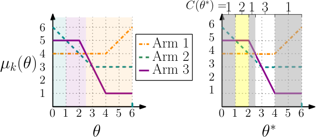
Empirical performance of Algorithm-C. In Figure 6 we compare the regret of Algorithm-C against the regret of Algorithm (UCB/TS/KL-UCB). We plot the cumulative regret attained under Algorithm-C vs. Algorithm of the example shown in Figure 5 for three different values of and . Refer to Figure 5 to see that , and for , and , respectively. Due to this, we see that Algorithm-C achieves bounded regret for , and reduced regret relative to Algorithm for as only one arm is pulled times. For , even though (i.e., all arms are competitive), Algorithm-C achieves empirically smaller regret than Algorithm. We also see the advantage of using TS-C and KL-UCB-C over UCB-C in Figure 6 as Thompson Sampling and KL-UCB are known to outperform UCB empirically. For all the simulations, we set . Rewards are drawn from the distribution , i.e, . We average the regret over experiments. For a given experiment, all algorithms use the same reward realizations.
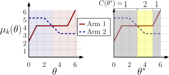
Performance comparison with UCB-S. In the first row of Figure 6, we also plot the performance of the UCB-S algorithm proposed in (Lattimore and Munos 2014), alongside UCB and UCB-C. The UCB-S algorithm constructs the confidence set just like UCB-C, and then in the next step selects the arm . Informally, it finds the maximum possible mean reward over for each arm . As a result, UCB-S tends to favor pulling arms that have the largest mean reward for . This bias renders the performance of UCB-S to depend heavily on . When , UCB-S has the smallest regret among the three algorithms compared in Figure 6, but when it gives even worse regret than UCB. A similar observation can be made in another simulation setting described below.
Figure 8 compares UCB, UCB-S, UCB-C and TS-C for the functions shown in Figure 7. We plot the cumulative regret after 50000 rounds for different values of and observe that TS-C performs the best for most values. As before, the performance of UCB-S varies significantly with . In particular, UCB-S has the smallest regret of all when , but achieves worse regret even compared to UCB when . On the other hand, our UCB-C performs better than or at least as good as UCB for all . While UCB-S also achieves the regret bound of 1, the ability to employ any Algorithm in the last step of Algorithm-C is a key advantage over UCB-S, as Thompson Sampling and KL-UCB can have significantly better empirical performance over UCB.
Comparison in linear bandit and multi-dimensional settings. As highlighted in Section 2, our problem formulation allows to be multi-dimensional as well. Figure 9 shows the performance of UCB-C and TS-C relative to GLM-UCB in a linear bandit setting. In a linear bandit setting, mean reward of arm is . Here is a vector associated with arm , which is known to the player. The parameter is unknown to the player, and hence it fits in our structured bandit framework. It is important to see that while UCB-C and TS-C are designed for a much broader class of problems, they still show competitive performance relative to specialized algorithms (i.e., GLM-UCB) in the linear bandit setting (Figure 9). Figure 10 shows a setting in which is multi-dimensional, but the reward mappings are non-linear and hence the setting is not captured through a linear bandit framework. Our results in Figure 10 demonstrate that the UCB-C and TS-C algorithms work in such settings as well while providing significant improvements over UCB in certain cases.
5.5 When do we get bounded regret?
When , all sub-optimal arms are pulled only times, leading to a bounded regret. Cases with can arise quite often in practical settings. For example, when functions are continuous or is countable, this occurs when the optimal arm is invertible, or has a unique maximum at , or any case where the set is a singleton. These cases lead to all sub-optimal arms being non-competitive, whence UCB-C achieves bounded (i.e., ) regret. There are more general scenarios where bounded regret is possible. To formally present such cases, we utilize a lower bound obtained in (Combes et al. 2017).
Proposition 1 (Lower bound).
For any uniformly good algorithm (Lai and Robbins 1985), and for any , we have:
An algorithm is uniformly good if for all and all . Here is the number of arms that are -Competitive, with being the set .
This suggests that bounded regret is possible only when and logarithmic regret is unavoidable in all other cases. The proof of this proposition follows from a bound derived in (Combes et al. 2017) and it is given in Appendix B.
There is a subtle difference between and . This arises in corner case situations when a -Non-Competitive arm is competitive. Note that the set can be interpreted as the confidence set obtained when we pull the optimal arm infinitely many times. In practice, if we sample the optimal arm a large number of times, we can only obtain the confidence set for some . Due to this, there is a difference between and . Consider the case shown in Figure 11 with . For , Arm 1 is optimal. In this case . For all values of , and hence Arm 2 is -Non-Competitive. However, for any , Arm 2 is -competitive and hence Competitive. Due to this, we have and in this case.
If is a countable set, a -Non-Competitive arm is always -Non-Competitive, that is, . This occurs because one can always choose so that a -Non-Competitive arm is also -Non-Competitive. This shows that when is a countable set (which is true for most practical situations where the hidden parameter is discrete), UCB-C achieves bounded regret whenever possible, that is, whenever . While this property holds true for the case when is a countable set, there can be more general cases where . Our algorithms and regret analysis are valid regardless of being countable or not.

6 Additional Exploration of Non-competitive But Informative Arms
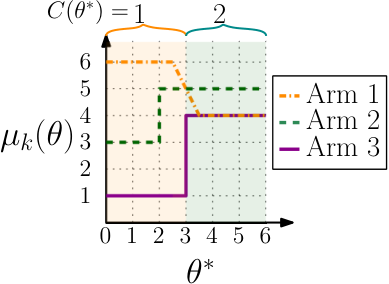
The previous discussion shows that the UCB-C and TS-C algorithms enable substantial reductions in the effective number of arms and the expected cumulative regret. A strength of the proposed algorithms that can be a weakness in some cases is that they stop pulling non-competitive arms that are unlikely to be optimal after some finite number of steps. Although an arm may be non-competitive in terms of its reward yield, it can be useful in inferring the hidden parameter , which in turn may help reduce the regret incurred in subsequent steps. For instance, consider the example shown in Figure 12. Here, Arm 3 is sub-optimal for all values of and is never pulled by UCB-C, but it can help identify whether or . Motivated by this, we propose an add-on to Algorithm-C, named as the Informative Algorithm-C (Algorithm 3), that takes the informativeness of arms into account and performs additional exploration of the most informative arm with a probability that decreases over time.
6.1 Informativeness of an Arm
Intuitively, an arm is informative if it helps us to obtain information about the hidden parameter . At the end of round , we know a confidence interval for the hidden parameter . We aim to quantify the informativeness of an arm with respect to this confidence set . For instance, if in Figure 12, we see that the reward function of Arm 3 has high variance and it suggests that the samples of Arm 3 could be helpful in knowing about . On the other hand, samples of Arm 2 will not be useful in identifying if . There can be several ways of defining the informativeness of an arm with respect to set . We consider the following two metrics in this paper.
KL-Divergence. Assuming that has a uniform distribution in , we can define the informativeness of an arm as the expected KL-Divergence between two samples of arm , i.e., . Our intuition here is that larger expected KL-divergence for an arm indicates that samples from it have substantially different distributions under different values, which in turn indicates that those samples will be useful in inferring the true value of . Assuming that is a Gaussian distribution with mean and variance , then the expected KL-Divergence can be simplified as
where, is the variance in the mean reward function , calculated when is uniformly distributed over the current confidence set . Observe that the metric is easy to evaluate given the functions and the confidence set obtained from Step 1.
Entropy. Alternatively, can be viewed as a derived random variable of , where is uniformly distributed over the current confidence set . The informativeness of arm can then be defined as . When is discrete this will be the Shannon entropy , while for continuous it will be the differential entropy where is the probability density function of the derived random variable . Observe that differential entropy takes into account the shape as well as the range of . For example, if two reward functions are linear in , the one with a higher slope will have higher differential entropy, as we would desire from an informativeness metric. Evaluating the differential entropy in , i.e., , can be computationally challenging.
Other than the two metrics described above, there might be alternative (and potentially more complicated) ways of quantifying the informativeness of an arm. Another candidate would be the information gain metric proposed in (Russo and Van Roy 2014), which defines informativeness in terms of identifying the best arm, rather than inferring . However, as already mentioned in (Russo and Van Roy 2014) by the authors, information gain is computationally challenging to implement in practice outside of certain specific class of problems where prior distribution of is Beta or Gaussian.
6.2 Proposed Informative Algorithm-C and its Expected Regret
Given an informativeness metric , we define the most informative arm for the confidence set as . At round , Informative Algorithm-C (described in Algorithm 3) picks the most informative arm with probability where , and otherwise uses UCB-C or TS-C to pull one of the competitive arms.Here, and are hyperparameters of the Informative UCB-C algorithm. Larger or small results in more exploration during the initial rounds. Setting the probability of pulling the most informative arm as ensures that the algorithm pulls the informative arms more frequently at the beginning. This helps shrink faster. Setting ensures that informative but non-competitive arms are only pulled times in expectation. Thus, asymptotically the algorithm will behave exactly as the underlying Algorithm-C and the regret of Informative-Algorithm-C is at most an constant worse than the Algorithm-C algorithm.
6.3 Simulation results
We implement two versions of Informative-Algorithm-C, namely Algorithm-C-KLdiv and Algorithm-C-Entropy, which use the KL-divergence and Entropy metrics respectively to identify the most informative arm at round . Algorithm-C-KLdiv picks the arm with highest variance in , i.e., . Algorithm-C-Entropy picks an arm whose mean reward function, , has largest shannon entropy for (assuming to be a uniform random variable in ). As a baseline for assessing the effectiveness of the informativeness metrics, we also implement Algorithm-C-Random which selects by sampling one of the arms uniformly at random from the set of all arms at round .
Figure 13 shows the cumulative regret of the aforementioned algorithms for the reward functions shown in Figure 12, where the hidden parameter . Among UCB-C, UCB-C-KLdiv, UCB-C-Entropy and UCB-C-Random, UCB-C-KLdiv has the smallest cumulative regret. This is because UCB-C-KLdiv identifies Arm 3 as the most informative arm, samples of which are helpful in identifying whether or . Hence, occasional pulls of Arm 3 lead to fast shrinkage of the set . In contrast to UCB-C-KLdiv, UCB-C-Entropy identifies Arm 2 as the most informative arm for , due to which UCB-C-Entropy samples Arm 2 more often in the initial stages of the algorithm. As the information obtained from Arm 2 is relatively less useful in deciding whether or not, we see that UCB-C-Entropy/TS-C-Entropy does not perform as well as UCB-C-KLdiv/TS-C-KLdiv in this scenario. UCB-C-Random picks the most informative arm by selecting an arm uniformly at random from the available set of arms. The additional exploration through random sampling is helpful, but the cumulative regret is larger than UCB-C-KLdiv as UCB-C-Random pulls Arm 3 fewer times relative to UCB-C-KLdiv. For this particular example, cumulative regret of UCB-S was 2500, whereas other UCB style algorithms achieve cumulative regret of 600-800 as shown in the Figure 13(a). This is due to the preference of UCB-S to pick Arm 1 in this example. We see similar trends among TS-C, TS-C-KLdiv, TS-C-Entropy and TS-C-Random. The cumulative regret is smaller for Thompson sampling variants as Thompson sampling is known to outperform UCB empirically.
We would like to highlight that the additional exploration by Informative-Algorithm-C is helpful only in cases where non-competitive arms help significantly shrink the confidence set . For the experimental setup presented in Section 7 below, the reward functions are mostly flat as seen in Appendix G and thus, Informative Algorithm-C does not give a significant improvement over the corresponding Algorithm-C. Therefore for clarity of the plots, we do not present experiments results for Informative-C in other settings of this paper.
7 Experiments with Movielens data
We now show the performance of UCB-C and TS-C on a real-world dataset. We use the Movielens dataset (Harper and Konstan 2015) to demonstrate how UCB-C and TS-C can be deployed in practice and demonstrate their superiority over classical UCB and TS. Since movie recommendations is one of many applications of structured bandits, we do not compare with methods such as collaborative filtering that are specific to recommendation systems. Also, we do not compare with contextual bandits since the structured bandit setting has a different goal of making recommendations without accessing a user’s contextual features.
The Movielens dataset contains a total of 1M ratings made by users for movies. There are different user types (based on having distinct age and occupation features) and different genres of movies. The users have given ratings to the movies on a scale of to . Each movie is associated with one (and in some cases, multiple) genres. For the experiments, of the possibly multiple genres for each movie, we choose one uniformly at random. The set of users that belong to a given type is referred to as a meta-user; thus there are different meta-users. These different meta-users correspond to the different values that the hidden parameter can take in our setting. For example, one of the meta-users in the data-set represents college students whose age is between and , and this corresponds to the case . We split the dataset into two equal parts, training and test. This split is done at random, while ensuring that the training dataset has samples from all meta-users.
For a particular meta-user whose features are unknown (i.e., the true value of is hidden), we need to sequentially choose one of the genres (i.e., one of the arms) and recommend a movie from that genre to the user. In doing so, our goal is to maximize the total rating given by this user to the movies we recommended. We use the training dataset ( of the whole data) to learn the mean reward mappings from meta-users () to different genres (arms); these mappings are shown in Appendix G. The learned mappings indicate that the mean-reward mappings of meta-users for different genres are related to one another. For example, on average 56+ year old retired users may like documentaries more than children’s movies. In our experiments, these dependencies are learned during the training. In practical settings of recommendations or advertising, these mappings can be learned from pilot surveys in which users participate with their consent.
We test the algorithm for three different meta-users, i.e., for three different values of . The movie rating samples for these meta-users are obtained from the test dataset, (the remaining of the data). Figure 14 shows that UCB-C and TS-C achieve significantly lower regret than UCB, TS as only a few arms are pulled times. This is because only of the sub-optimal arms are pulled times by our UCB-C and TS-C algorithms. For our experimental setting, the value of depends on (which is unknown to the algorithm). Figure 15 shows how varies with , where it is seen that is significantly smaller than for all . As a result, the performance improvements observed in Figure 14 for our UCB-C and TS-C algorithms will apply to other values as well. There are values for which UCB-C is better than UCB-S, and vice versa. But, TS-C always outperforms UCB-C and UCB-S in our experiments. We tried Informative UCB-C in this setting as well, but the results were similar to that of UCB-C because the arms in this setting are not too informative.
8 Concluding Remarks
In this work, we studied a structured bandit problem in which the mean rewards of different arms are related through a common hidden parameter. Our problem setting makes no assumptions on mean reward functions, due to which it subsumes several previously studied frameworks Atan et al. 2015; Wang et al. 2018; Mersereau et al. 2009. We developed an approach that allows us to extend a classical bandit Algorithm to the structured bandit setting, which we refer to as Algorithm-C. We provide a regret analysis of UCB-C (structured bandit versions of UCB). A key insight from this analysis is that Algorithm-C pulls only of the sub-optimal arms times and all other arms, termed as non-competitive arms, are pulled only times. Through experiments on the Movielens dataset, we demonstrated that UCB-C and TS-C give significant improvements in regret as compared to previously proposed approaches. Thus, the main implication of this paper is that it provides a unified approach to exploit the structured rewards to drastically reduce exploration in a principled manner.
For cases where non-competitive arms can provide information about that can shrink the confidence set , we propose a variant of Algorithm-C called informative-Algorithm-C that takes the informativeness of arms into account without increasing unnecessary exploration. Linear bandit algorithms Abbasi-Yadkori et al. 2011; Filippi et al. 2010; Lattimore and Szepesvari 2016 shrink the confidence set in a better manner by taking advantage of the linearity of the mean reward functions to estimate as the solution to least squares problem Abbasi-Yadkori et al. 2011. Moreover, linearity helps them to use self-normalized concentration bound for vector valued martingale, (Theorem 1 in Abbasi-Yadkori et al. 2011) to construct the confidence intervals. Extending this approach to the general structured bandit setting is a non-trivial open question due to the absence of constraints on the nature of mean reward functions . The paper Combes et al. 2017 proposes a statistical hypothesis testing method for the case of known conditional reward distributions. Generalizing it to the setting considered in this paper is an open future direction. While we state our results for a scenario where mean reward functions are known, our algorithmic approach, analysis and results can also be extended to a setting where only lower and upper bounds on the mean reward function are known. This setting is discussed in Appendix A. Another open direction in this field is to study the problem of structured best-arm identification where the goal is to conduct pure exploration and identify the best arm in the fewest number of rounds.
References
- Abbasi-Yadkori et al. (2011) Yasin Abbasi-Yadkori, Dávid Pál, and Csaba Szepesvári. Improved algorithms for linear stochastic bandits. In Advances in Neural Information Processing Systems, pages 2312–2320, 2011.
- Agrawal and Goyal (2012) Shipra Agrawal and Navin Goyal. Analysis of thompson sampling for the multi-armed bandit problem. In Conference on Learning Theory, pages 39–1, 2012.
- Agrawal and Goyal (2013a) Shipra Agrawal and Navin Goyal. Further optimal regret bounds for thompson sampling. In Artificial Intelligence and Statistics, pages 99–107, 2013a.
- Agrawal and Goyal (2013b) Shipra Agrawal and Navin Goyal. Thompson sampling for contextual bandits with linear payoffs. In Proceedings of the International Conference on Machine Learning (ICML), 2013b. URL http://dl.acm.org/citation.cfm?id=3042817.3043073.
- Atan et al. (2015) Onur Atan, Cem Tekin, and Mihaela van der Schaar. Global multi-armed bandits with Hölder continuity. In AISTATS, 2015.
- Audibert et al. (2010) Jean-Yves Audibert, Sebastien Bubeck, and Rémi Munosr. Best arm identification in multi-armed bandits. In Proceedings of the annual Conference On Learning Theory (COLT), pages 359–376, 2010.
- Auer et al. (2002) Peter Auer, Nicolo Cesa-Bianchi, and Paul Fischer. Finite-time analysis of the multiarmed bandit problem. Machine learning, 47(2-3):235–256, 2002.
- Bubeck et al. (2009) Sébastien Bubeck, Rémi Munos, and Gilles Stoltz. Pure exploration in multi-armed bandits problems. In Ricard Gavaldà, Gábor Lugosi, Thomas Zeugmann, and Sandra Zilles, editors, Algorithmic Learning Theory, pages 23–37, Berlin, Heidelberg, 2009. Springer Berlin Heidelberg.
- Bubeck et al. (2012) Sébastien Bubeck, Nicolo Cesa-Bianchi, et al. Regret analysis of stochastic and nonstochastic multi-armed bandit problems. Foundations and Trends in Machine Learning, 5(1):1–122, 2012.
- Chapelle and Li (2011) Olivier Chapelle and Lihong Li. An empirical evaluation of thompson sampling. In J. Shawe-Taylor, R. S. Zemel, P. L. Bartlett, F. Pereira, and K. Q. Weinberger, editors, Advances in Neural Information Processing Systems, pages 2249–2257, 2011.
- Combes et al. (2017) Richard Combes, Stefan Magureanu, and Alexandre Proutière. Minimal exploration in structured stochastic bandits. In NIPS, 2017.
- Filippi et al. (2010) Sarah Filippi, Olivier Cappe, Aurélien Garivier, and Csaba Szepesvári. Parametric bandits: The generalized linear case. In Advances in Neural Information Processing Systems, pages 586–594, 2010.
- Gabillon et al. (2012) Victor Gabillon, Mohammad Ghavamzadeh, and Alessandro Lazaric. Best arm identification: A unified approach to fixed budget and fixed confidence. In Advances in Neural Information Processing Systems, pages 3212–3220, 2012.
- Garivier and Cappé (2011) Aurélien Garivier and Olivier Cappé. The kl-ucb algorithm for bounded stochastic bandits and beyond. In Proceedings of the 24th annual Conference On Learning Theory, pages 359–376, 2011.
- Garivier and Kaufmann (2016) Aurélien Garivier and Emilie Kaufmann. Optimal best arm identification with fixed confidence. In Annual Conference on Learning Theory (COLT), volume 49 of Proceedings of Machine Learning Research, pages 998–1027, Columbia University, New York, New York, USA, 23–26 Jun 2016. PMLR. URL http://proceedings.mlr.press/v49/garivier16a.html.
- Gopalan et al. (2014) Aditya Gopalan, Shie Mannor, and Yishay Mansour. Thompson sampling for complex online problems. In Proceedings of the 31st International Conference on Machine Learning, volume 32 of Proceedings of Machine Learning Research, pages 100–108, Bejing, China, 22–24 Jun 2014. PMLR. URL http://proceedings.mlr.press/v32/gopalan14.html.
- Graves and Lai (1997) Todd L Graves and Tze Leung Lai. Asymptotically efficient adaptive choice of control laws incontrolled markov chains. SIAM journal on control and optimization, 35(3):715–743, 1997.
- Harper and Konstan (2015) F. Maxwell Harper and Joseph A. Konstan. The movielens datasets: History and context. ACM Transactions on Interactive Intelligent Systems (TiiS), 5, 4, Article 19, 2015.
- Heckel et al. (2016) Reinhard Heckel, Nihar B. Shah, Kannan Ramchandran, and Martin J. Wainwright. Active ranking from pairwise comparisons and the futility of parametric assumptions. arXiv, abs/1606.08842, 2016. URL http://arxiv.org/abs/1606.08842.
- Huang et al. (2017) Ruitong Huang, Mohammad M. Ajallooeian, Csaba Szepesvári, and Martin Müller. Structured best arm identification with fixed confidence. In Proceedings of the International Conference on Algorithmic Learning Theory (ALT), volume 76 of Proceedings of Machine Learning Research, pages 593–616, Kyoto University, Kyoto, Japan, October 2017. URL http://proceedings.mlr.press/v76/huang17a.html.
- Jamieson and Nowak (2014) K. Jamieson and R. Nowak. Best-arm identification algorithms for multi-armed bandits in the fixed confidence setting. In Proceedings on the Annual Conference on Information Sciences and Systems (CISS), pages 1–6, March 2014.
- Jamieson et al. (2014) Kevin Jamieson, Matthew Malloy, Robert Nowak, and Sébastien Bubeck. lil’ucb: An optimal exploration algorithm for multi-armed bandits. In Conference on Learning Theory, pages 423–439, 2014.
- Jamieson et al. (2015) Kevin G Jamieson, Lalit Jain, Chris Fernandez, Nicholas J Glattard, and Rob Nowak. Next: A system for real-world development, evaluation, and application of active learning. In Advances in Neural Information Processing Systems, pages 2656–2664, 2015.
- Kaufmann et al. (2016) Emilie Kaufmann, Olivier Cappé, and Aurélien Garivier. On the complexity of best-arm identification in multi-armed bandit models. The Journal of Machine Learning Research, 17(1):1–42, 2016.
- Lai and Robbins (1985) Tze Leung Lai and Herbert Robbins. Asymptotically efficient adaptive allocation rules. Advances in applied mathematics, 6(1):4–22, 1985.
- Lattimore and Munos (2014) Tor Lattimore and Rémi Munos. Bounded regret for finite-armed structured bandits. In Advances in Neural Information Processing Systems, pages 550–558, 2014.
- Lattimore and Szepesvari (2016) Tor Lattimore and Csaba Szepesvari. The end of optimism? an asymptotic analysis of finite-armed linear bandits. arXiv preprint arXiv:1610.04491, 2016.
- Li et al. (2010) Lihong Li, Wei Chu, John Langford, and Robert E Schapire. A contextual-bandit approach to personalized news article recommendation. In Proceedings of the 19th international conference on World wide web, pages 661–670. ACM, 2010.
- Li et al. (2017) Lisha Li, Kevin Jamieson, Giulia DeSalvo, Afshin Rostamizadeh, and Ameet Talwalkar. Hyperband: A novel bandit-based approach to hyperparameter optimization. Journal of Machine Learning Research, 18(1):6765–6816, January 2017. ISSN 1532-4435. URL http://dl.acm.org/citation.cfm?id=3122009.3242042.
- Mannor and Tsitsiklis (2004) Shie Mannor and John N Tsitsiklis. The sample complexity of exploration in the multi-armed bandit problem. Journal of Machine Learning Research, 5(Jun):623–648, 2004.
- Mersereau et al. (2009) A. J. Mersereau, P. Rusmevichientong, and J. N. Tsitsiklis. A structured multi-armed bandit problem and the greedy policy. IEEE Transactions on Automatic Control, 54(12):2787–2802, Dec 2009. ISSN 0018-9286. doi: 10.1109/TAC.2009.2031725.
- Nino-Mora (2009) J. Nino-Mora. Stochastic scheduling. In Encyclopedia of Optimization, pages 3818–3824. Springer, New York, 2 edition, 2009.
- Russo and Van Roy (2014) Daniel Russo and Benjamin Van Roy. Learning to optimize via posterior sampling. Mathematics of Operations Research, 39(4):1221–1243, 2014.
- Russo et al. (2017) Daniel Russo, Benjamin Van Roy, Abbas Kazerouni, and Ian Osband. A tutorial on thompson sampling. CoRR, abs/1707.02038, 2017. URL http://arxiv.org/abs/1707.02038.
- Sen et al. (2017) Rajat Sen, Karthikeyan Shanmugam, Alexandros G Dimakis, and Sanjay Shakkottai. Identifying best interventions through online importance sampling. stat, 1050:9, 2017.
- Sen et al. (2018) Rajat Sen, Karthikeyan Shanmugam, and Sanjay Shakkottai. Contextual bandits with stochastic experts. In Proceedings of the Twenty-First International Conference on Artificial Intelligence and Statistics, volume 84 of Proceedings of Machine Learning Research, pages 852–861, 2018. URL http://proceedings.mlr.press/v84/sen18a.html.
- Shen et al. (2018) Cong Shen, Ruida Zhou, Cem Tekin, and Mihaela van der Schaar. Generalized global bandit and its application in cellular coverage optimization. IEEE Journal of Selected Topics in Signal Processing, 12(1):218–232, 2018.
- Soare et al. (2014) Marta Soare, Alessandro Lazaric, and Remi Munos. Best-arm identification in linear bandits. In Advances in Neural Information Processing Systems (NIPS), pages 828–836. 2014. URL http://papers.nips.cc/paper/5460-best-arm-identification-in-linear-bandits.pdf.
- Tánczos et al. (2017) Ervin Tánczos, Robert Nowak, and Bob Mankoff. A kl-lucb algorithm for large-scale crowdsourcing. In Advances in Neural Information Processing Systems, pages 5894–5903, 2017.
- Tao et al. (2018) Chao Tao, Saúl Blanco, and Yuan Zhou. Best arm identification in linear bandits with linear dimension dependency. In Proceedings of the International Conference on Machine Learning (ICML), volume 80 of Proceedings of Machine Learning Research, pages 4877–4886, July 2018. URL http://proceedings.mlr.press/v80/tao18a.html.
- Tekin and Turgay (2017) Cem Tekin and Eralp Turgay. Multi-objective contextual multi-armed bandit problem with a dominant objective. arXiv preprint arXiv:1708.05655, 2017.
- Thompson (1933) W. R. Thompson. On the Likelihood that One Unknown Probability Exceeds Another in View of the Evidence of Two Samples. Biometrika, 25(3-4):285–294, December 1933.
- Villar et al. (2015) Sofía S Villar, Jack Bowden, and James Wason. Multi-armed bandit models for the optimal design of clinical trials: benefits and challenges. Statistical science: a review journal of the Institute of Mathematical Statistics, 30(2):199, 2015.
- Wang et al. (2018) Zhiyang Wang, Ruida Zhou, and Cong Shen. Regional multi-armed bandits. In AISTATS, 2018.
- White (2012) John White. Bandit algorithms for website optimization. " O’Reilly Media, Inc.", 2012.
Appendix A Noisy mean reward functions
Throughout the work we assume that the mean reward functions are known exactly. Consider a scenario where only partial information is known about the mean reward functions . We show in this section that our proposed algorithmic approach is flexible enough to accommodate for such scenarios. The flexibility in our framework can be maintained as long as we have some upper and lower bound on mean reward functions. Suppose the mean reward functions are noisy, but it is known that . In such a case, we can alter the definition of as follows,
where and are defined as follows,
Subsequently, we call an arm to be Non-Competitive if for all . On doing so, our algorithmic approach can be extended to this framework as well. Additionally, we can re-define the notion of non-competitive and competitive arms in this setting as follows.
Definition 5 (Non-Competitive and Competitive arms in the noisy setting).
For any , let
An arm is said to be non-competitive if there exists an such that for all . Otherwise, the arm is said to be competitive; i.e., if for all , such that . The number of competitive arms is denoted by .
After doing so, the analysis can be easily extended to prove the desired regret bounds in this setting. In particular, one can show that , and subsequently all other results of our paper will follow through. As there is lesser information in this newer framework, one can expect the number of competitive arms to be greater than the number of competitive arms in the setting where . As the algorithm, results and analysis can extend beyond the framework described in the paper, it makes our proposed approach even more promising.
Appendix B Lower bound: Proof for Proposition 1
Proof for Proposition 1 We use the following result of (Combes et al. 2017) to state Proposition 1.
Theorem 4 (Lower bound, Theorem 1 in Combes et al. 2017.).
For any uniformly good algorithm (Lai and Robbins 1985), and for any , we have:
where is the solution of the optimization problem:
| (9) | ||||
Here, is the KL-Divergence between distributions and . An algorithm, , is uniformly good if for all and all .
We see that the solution to the optimization problem (9) is only when the set is empty. The set being empty corresponds to a case where all sub-optimal arms are -non-competitive. This implies that sub-logarithmic regret is possible only when , i.e there is only one -competitive arm, which is the optimal arm, and all other arms are non-competitive. It is assumed that reward distribution of an arm is parameterized by the mean of arm ; this ensures that if then we have .
Appendix C Results valid for any Algorithm-C
We now present results that depend only on Step 1 and Step 2 of our algorithm and hence are valid for any Algorithm-C, where Algorithm can be UCB, Thompson sampling or any other method designed for classical multi-armed bandits with independent arms.
Fact 1 (Hoeffding’s inequality).
Let be i.i.d. random variables, where is sub-gaussian with mean , then
Here is the empirical mean of the .
Lemma 1 (Standard result used in bandit literature (Used in Theorem 2.1 of Auer et al. 2002)).
If denotes the empirical mean of arm by pulling arm times through any algorithm and denotes the mean reward of arm , then we have
Proof.
Let be the reward samples of arm drawn separately. If the algorithm chooses to play arm for time, then it observes reward . Then the probability of observing the event can be upper bounded as follows,
| (10) |
| (11) |
∎
Lemma 2.
The probability that the difference between the true mean of arm and its empirical mean after time slots is more than is upper bounded by , i.e.,
Proof.
Lemma 3.
Define to be the event that arm is -non-competitive for the round , then,
Proof.
Observe that
| (14) |
| (15) | ||||
| (16) | ||||
| (17) | ||||
In order for Arm to be -non-competitive, we need . See that implies that arm is -Competitive. Therefore, is a necessary condition for Arm to be -Non-Competitive. Due to this, we have in (14). We are using to denote the empirical mean of rewards from arm obtained from it’s pulls. Here (14) follows from definition of confidence set and (15) follows from union bound. We have (16) from union bound and is a standard trick to deal with the random variable as it can take values from to (1). The inequality (17) follows from Hoeffding’s lemma. ∎
Lemma 4.
Consider a suboptimal arm , which is -non-competitive. If for some constant , then,
where .
Proof.
We now bound this probability as,
| (18) | ||||
| (19) | ||||
| (20) |
See that for . This holds as and if , then . Therefore in order for arm to be -competitive, we need at least , which leads to (18) as arm is non-competitive. Inequality (19) follows from Hoeffding’s inequality. The term before the exponent in (19) arises as the random variable can take values from to (1). ∎
Appendix D Unified Regret Analysis
In this section, we show a sketch of how regret analysis of Algorithm-C can be performed, where Algorithm is a bandit algorithm that works for classical multi-armed bandit problem. In later section, we provide rigorous proof for the regret analysis of the UCB-C algorithm.
Bound on expected number of pulls for Non-Competitive arms
For non-competitive arms, we show that the expected number of pulls is . Intuition behind the proof of the result is that non-competitive arms can be identified as sub-optimal based on enough pulls of the optimal arm, due to which pulling a sub-optimal arm becomes unnecessary and it ends up being pulled only times. We now provide a mathematical proof sketch of this idea:
We bound as
| (21) | ||||
| (22) |
In order to prove that Algorithm-C achieves bounded regret, we need to show that for some . Intuitively, this means that the probability of selecting a sub-optimal arm more than times decays with the number of rounds. This property should intuitively hold true for any good performing bandit algorithm. We prove this rigorously for UCB-C.
Bound on expected number of pulls for Competitive arms
For any suboptimal arm ,
| (23) | ||||
| (24) |
Here Equation 24 follows from the result of 3 with being the event that arm is -non-competitive for the round .
See that the event corresponds to the event that a sub-optimal arm and optimal arm are both present in the competitive set, and the Algorithm selects the sub-optimal arm . The analysis of this term is exactly equivalent to selecting a sub-optimal arm over optimal arm by Algorithm. This leads to a bound on the expected pulls of the competitive arms as classical bandit algorithms pull each arm times.
Appendix E Proof for the UCB-C Algorithm
Lemma 5.
If for some constant then,
where is a suboptimal arm.
Proof.
The probability that arm is pulled at step , given it has been pulled times can be bounded as follows:
| (25) | ||||
| (26) |
Here, (25) follows from union bound and (26) follows from 3. We now bound the second term as,
| (27) | ||||
| (28) | ||||
| (29) | ||||
| (30) | ||||
| (31) |
Equation (27) follows from the fact that . Inequality (28) arrives from dropping and in the previous expression. We have (29) from 2 and the fact that Inequality (30) follows from the Hoeffding’s inequality and the term before the exponent in (30) arises as the random variable,, can take values between and (1). Equation (31) results from the definition of and the fact that .
∎
Lemma 6.
Let be the minimum integer satisfying then , and , we have,
Proof.
This gives us that , we have,
Now consider the summation
This gives us,
Since , we have,
∎
Proof of Theorem 3 For any sub-optimal arm ,
| (35) | ||||
| (36) | ||||
| (37) |
Here, (36) follows from 3. We have (37) from the analysis of UCB for the classical bandit problem. This is because the term counts the number of times and , which is the exact same term counted in the analysis of the UCB algorithm (Auer et al. 2002) to bound the expected number of pulls of arm . In particular, we can see from analysis of Theorem 1 in (Auer et al. 2002) (equivalently analysis of Theorem 2.1 in Bubeck et al. 2012) that and the event can happen only at-most times. (Auer et al. 2002) does this analysis for bounded random variables (i.e., ) and in their proof of Theorem 1. The analysis is replicated in the proof of Theorem 2.1 in (Bubeck et al. 2012) for a general . For further details we refer the reader to the analysis of UCB done in Theorem 2.1 of (Bubeck et al. 2012).
Appendix F Regret analysis for the TS-C Algorithm
We now present results for TS-C in the scenario where and Thompson sampling is employed with Beta priors (Agrawal and Goyal 2013a). In order to prove results for TS-C, we assume that rewards are either or . The Thompson sampling algorithm with beta prior, maintains a posterior distribution on mean of arm as . Subsequently, it generates a sample for each arm and selects the arm . The TS-C algorithm with Beta prior uses this Thompson sampling procedure in its last step, i.e., , where is the set of -Competitive arms at round . We show that in a 2-armed bandit problem, the regret is if the sub-optimal arm is non-competitive and is otherwise.
For the purpose of regret analysis of TS-C, we define two thresholds, a lower threshold , and an upper threshold for arm ,
| (38) |
Let and be the events that,
| (39) |
To analyse the regret of TS-C, we first show that the number of times arm is pulled jointly with the event that is bounded above by an constant, which is independent of the total number of rounds .
Lemma 7.
If for some constant , then,
where is a sub-optimal arm.
Proof.
We start by bounding the probability of the pull of -th arm at round as follows,
| (40) |
where , comes from 3. Now we treat each term in (40) individually. To bound term A, we note that . From the analysis in (Agrawal and Goyal 2013a) (equation 6), we see that
as it is shown through Lemma 2 in (Agrawal and Goyal 2013a) that,
.
Here, .
Due to this,
.
We now bound the sum of term B from to by noting that
. Additionally, from Lemma 3 in (Agrawal and Goyal 2013a), we get that
, where . As a result, we see that
.
Finally, for the last term C we can show that,
| (42) | ||||
Here Equation 42 follows from hoeffding’s inequality and the union bound trick to handle random variable . After plugging these results in (40), we get that
| (43) | ||||
| (44) | ||||
| (45) |
∎
We now show that the expected number of pulls by TS-C for a non-competitive arm is bounded above by an constant.
Expected number of pulls by TS-C for a non-competitive arm.
We bound as
| (46) | ||||
| (47) | ||||
| (48) |
Here, (47) follows from 4 and (48) follows from 7 and the fact that the sum of is bounded for and
We now show that when the sub-optimal arm is competitive, the expected pulls of arm is .
Expected number of pulls by TS-C for a competitive arm .: For any sub-optimal arm ,
| (49) | ||||
| (50) | ||||
| (51) | ||||
| (52) |
Here, (50) follows from 3. We have (51) from the analysis of Thompson Sampling for the classical bandit problem in (Agrawal and Goyal 2013a). This arises as the term counts the number of times and . This is precisely the term analysed in Theorem 3 of (Agrawal and Goyal 2013a) to bound the expected pulls of sub-optimal arms by TS. In particular, (Agrawal and Goyal 2013a) analyzes the expected number of pull of sub-optimal arm (termed as in their paper) by evaluating and it is shown in their Section 2.1 (proof of Theorem 1 of (Agrawal and Goyal 2013a)) that . The term is equivalent to and is equal to in our notations. Moreover , giving us the desired result of (51).
Appendix G Reward functions for the experiments
As mentioned in Section 7, we use a part of the Movielens dataset () as the training dataset, on which the mean reward mappings from meta-users to different genres are learned. Figure 16 represents the learned mappings on the training dataset.