Expectation Propagation for Poisson Data
Abstract
The Poisson distribution arises naturally when dealing with data involving counts, and it has found many applications in inverse problems and imaging. In this work, we develop an approximate Bayesian inference technique based on expectation propagation for approximating the posterior distribution formed from the Poisson likelihood function and a Laplace type prior distribution, e.g., the anisotropic total variation prior. The approach iteratively yields a Gaussian approximation, and at each iteration, it updates the Gaussian approximation to one factor of the posterior distribution by moment matching. We derive explicit update formulas in terms of one-dimensional integrals, and also discuss stable and efficient quadrature rules for evaluating these integrals. The method is showcased on two-dimensional PET images.
Keywords: Poisson distribution, Laplace prior, expectation propagation, approximate Bayesian inference
1 Introduction
The Poisson distribution is widely employed to describe inverse and imaging problems involving count data, e.g., emission computed tomography [44, 40], including positron emission tomography and single photon emission computed tomography. The corresponding likelihood function is a Poisson distribution with its parameter given by an affine transform (followed by a suitable link function). Over the past few decades, the mathematical theory and numerical algorithms for image reconstruction with Poisson data have witnessed impressive progresses. We refer interested readers to [22] for a comprehensive overview on variational regularization techniques for Poisson data and [4] for mathematical modeling and numerical methods for Poisson data. It is worth noting that the Poisson model is especially important in the low-count regime, e.g., photons, whereas in the moderate (or high) count regime, heteroscedastic normal approximations can be employed in the reconstruction, leading to a weighted Gaussian likelihood function (e.g., via the so-called Anscombe transform [2]). In this work, we focus on the Poisson model.
To cope with the inherent ill-posed nature of the imaging problem, regularization plays an important role in image reconstruction. This can be achieved implicitly via early stopping during an iterative reconstruction procedure (e.g., EM algorithm or Richardson-Lucy iterations) or explicitly via suitable penalties, e.g., Sobolev penalty, sparsity and total variation. The penalized maximum likelihood (or equivalently maximum a posteriori (MAP)) is currently the most popular way for image reconstruction with Poisson models [12, 41]. However, these approaches can only provide point estimates, and the important issue of uncertainty quantification, which provides crucial reliability assessment on point estimates, is not fully addressed. The full Bayesian approach provides a principled yet very flexible framework for uncertainty quantification of inverse and imaging problems [27, 42]. The prior distribution acts as a regularizer, and the ill-posedness of the imaging problem is naturally dealt with. Due to the imprecise prior knowledge of the solution and the presence of the data noise, the posterior distribution contains an ensemble of inverse solutions consistent with the observed data, which can be used to quantify the uncertainties associated with a point estimator, via, e.g., credible interval or highest probability density regions.
For imaging problems with Poisson data, a full Bayesian treatment is challenging, due to the nonnegativity constraint and high-dimensionality of the parameter / data space. There are several possible strategies from the computational perspective. One idea is to use general-purposed sampling methods to explore the posterior state space, predominantly Markov chain Monte Carlo (MCMC) methods [32, 37]. Recent scalable variants, e.g., stochastic gradient Langevin dynamics [47], are very promising, although these techniques have not been applied to the Poisson model. Then the constraints on the signal can be incorporated directly by discarding samples violating the constraint. However, in order to obtain accurate statistical estimates, sampling methods generally require many samples and thus tend to suffer from high computational cost, due to the high problem dimensionality. Further, the MCMC convergence is challenging to diagnose. These observations have motivated intensive research works on developing approximate inference techniques (AITs). In the machine learning literature, a large number of AITs have been proposed, e.g., variational inference [26, 6, 9, 24, 3], expectation propagation [34, 33] and more recently Bayesian (deep) neural network [17]; see the survey [48] for a comprehensive overview of recent developments on variational inference. In all AITs, one aims at finding an optimal approximate yet tractable distribution within a family of parametric/nonparametric probability distributions (e.g., Gaussian), by minimizing the error in a certain probability metric, prominently Kullback-Leibler divergence. Empirically they can often produce reasonable approximations but at a much reduced computational cost than MCMC. However, there seem no systematic strategies for handling constraints in these approaches. For example, a straightforward truncation of the distribution due to the constraint often leads to elaborated distributions, e.g., truncated normal distribution, which tends to make the computation tedious or even completely intractable in variational Bayesian inference.
In this work, we develop a computational strategy for exploring the posterior distribution for Poisson data (with two popular nonnegativity constraints) with a Laplace type prior based on expectation propagation [34, 33], in order to deliver a Gaussian approximation. Laplace prior promotes the sparsity of the image in a transformed domain, which is a valid assumption on most natural images. The main contributions of the work are as follows. First, we derive explicit update formulas using one-dimensional integrals. It essentially exploits the rank-one projection form of the factors to reduce the intractable high-dimensional integrals to tractable one-dimensional ones. In this way, we arrive at two approximate inference algorithms, parameterized by either moment or natural parameters. Second, we derive stable and efficient quadrature rules for evaluating the resulting one-dimensional integrals, i.e., a recursive scheme for Poisson sites with large counts and an approximate expansion for Laplace sites, and discuss different schemes for the recursion, dependent of the integration interval, in order to achieve good numerical stability. Last, we illustrate the approach with comprehensive numerical experiments with the posterior distribution formed by Poisson likelihood and an anisotropic total variation prior, clearly showcasing the feasibility of the approach.
Last, we put the work in the context of Bayesian analysis of Poisson data. The predominant body of literature in statistics employs a log link function, commonly known as Poisson regression in statistics and machine learning (see, e.g., [8, 3]). This differs substantially from the one frequently arising in medical imaging, e.g., positron emission tomography, and in particular the crucial nonnegativity constraint becomes vacuous. The only directly relevant work we are aware of is the recent work [28]. The work [28] discussed a full Bayesian exploration with EP, by modifying the posterior distributions using a rectified linear function on the transformed domain of the signal, which induces singular measures on the region violating the constraint. However, the work [28] does not consider the background.
The rest of the paper is organized as follows. In Section 2 we describe the posterior distribution for the Poisson likelihood function and a Laplace type prior. Then we give explicit expressions of the integrals involved in EP update and describe two algorithms in Section 3. In Section 4 we present stable and efficient numerical methods for evaluating one-dimensional integrals. Last, in Section 5 we present numerical results for three benchmark images. In the appendices, we describe two useful parameterizations of a Gaussian distribution, Laplace approximation and additional comparative numerical results for a one-dimensional problem with MCMC and Laplace approximation to shed further insights into the performance of EP algorithms.
2 Problem formulation
In this part, we give the Bayesian formulation for Poisson data, i.e., the likelihood function and prior distribution , and discuss the nonnegativity constraint.
Let be the (unknown) signal/image of interest, be the observed Poisson data, and be the forward map, where the superscript denotes matrix / vector transpose. The entries of the matrix are assumed to be nonnegative. For example, in emission computed tomography, it can be a discrete analogue of Radon transform, or probabilistically, the entry of the matrix denotes the probability that the th sensor pair records the photon emitted at the th site.
The conditional probability density of observing given the signal is given by
where is the background. That is, the entry follows a Poisson distribution with a parameter . The Poisson model of this form is popular in the statistical modeling of inverse and imaging problems involving counts, e.g., positron emission tomography [44]. If the entries of are independent and identically distributed (i.i.d.), then the likelihood function is given by
| (2.1) |
Note that the likelihood function is not well-defined for all , and suitable constraints on are needed in order to ensure the well-definedness of the factors ’s. In the literature, there are three popular constraints:
- 1.
;
- 2.
;
- 3.
.
Since the entries of are nonnegative, there holds . In practice, the first assumption is most consistent with the physics in that it reflects the physical constraint that emission counts are non-negative. The last two assumptions were proposed to reduce positive bias in the cold region [30], i.e., the region that has zero count. In this work, we shall focus on the last two constraints.
The constraints and can be unified, which is useful for the discussions below.
Definition 2.1.
For each likelihood factor with the constraint , let
For each likelihood factor with the constraint , let
| (2.2) |
Then the constraints and are both given by and .
With the indicator function of the set , we modify the likelihood function by
| (2.3) |
This extends the domain of from to , and it facilitates a full Bayesian treatment. Since the indicator function admits a separable form, i.e., , factorizes into
| (2.4) |
To fully specify the Bayesian model, we have to stipulate the prior . We focus on a Laplace type prior. Let and be the th row of . Then a Laplace type prior is given by
| (2.5) |
The parameter determines the strength of the prior, playing the role of a regularization parameter in variational regularization [23]. The choice of the hyperparameter in the prior is notoriously challenging [23]. One may apply hierarchical Bayesian modeling in order to estimate it from the data simultaneously with [46, 25, 3]. The prior is commonly known as a sparsity prior (in the transformed domain), which favors a candidate with many small elements and few large elements in the vector . The canonical total variation prior is recovered when the matrix computes the discrete gradient. It is well known that the total variation penalty can preserve well edges in the image/signals, and hence it has been very popular for various imaging tasks [38, 10].
By Bayes’ formula, we obtain the Bayesian solution to the Poisson inverse problem, i.e., the posterior probability density function:
| (2.6) |
where is the normalizing constant, defined by The computation of is generally intractable for high-dimensional problems, and has to be approximated.
3 Approximate inference by expectation propagation
In this section, we describe the basic concepts and algorithms of expectation propagation (EP), for exploring the posterior distribution (2.6). EP due to Minka [34, 33] is a popular variational type approximate inference method in the machine learning literature. It is especially suitable for approximating a distribution formed by a product of functions, with each factor being of projection form. Since its first appearance in 2001, EP has found many successful applications in practice, and it is reported to be very accurate, e.g., for Gaussian processes [36], and electrical impedance tomography with sparsity prior [19]. However, the theoretical understanding of EP remains quite limited [14, 13].
EP looks for an approximate Gaussian distribution to a target distribution by means of an iterative algorithm. It relies on the following factorization of the posterior distribution (with being the total number of factors):
| (3.1) |
Note that each factor is a function defined on the whole space . Likewise, we denote the Gaussian approximation to the posterior distribution by
with each factor being a Gaussian distribution , and is the corresponding normalizing constant. Below we use two different parameterizations of a Gaussian distribution, i.e., moment parameters (mean and covariance) and natural parameters ; see Appendix A. Both parameterizations have their pros and cons: the moment one does not require solving linear systems, and the natural one allows singular covariances for the Gaussians . The rest of this section is devoted to the derivation of the algorithms and their complexity.
3.1 Reduction to one-dimensional integrals
There are two main steps of one EP iteration: (a) form a tilted distribution , and (b) update the Gaussian approximation by matching its moments with that of . The moment matching step can be interpreted as minimizing Kullback-Leilber divergence [34, 33, 19]. Recall that the Kullback-Leibler divergence from one probability distribution to another is defined by [29]
| (3.2) |
By Jensen’s inequality, the divergence is always nonnegative, and it vanishes if and only if almost everywhere.
The task at step (a) is to construct the th tilted distribution . Let be the th cavity distribution, i.e., the product of all but the th factor, and defined by
| (3.3) |
with . It is Gaussian, i.e., , whose moment and natural parameters are denoted by and , respectively. Then the th tilted distribution of the approximation is given by
| (3.4) |
where is the corresponding normalizing constant. With the exclusion-inclusion step, one replaces the th factor in the approximation with the exact one .
The task at step (b) is to compute moments of the th tilde distribution , which are then used to update the approximation . This requires integration over , which is generally numerically intractable, if were arbitrary. Fortunately, each factor in (3.1) is of projection form and depends only on the scalar , with the vector being either or . This is the key fact rendering relevant high-dimensional integrals numerically tractable. Below we write the factor as and accordingly, the th cavity function as
| (3.5) |
upon replacing with its normalized version , and accordingly the normalizing constant .
Since a Gaussian is determined by its mean and covariance, it suffices to evaluate the 0th to 2nd moments of . The projection form of the factor allows reducing the moment evaluation of to 1D integrals. Theorem 3.1 gives the update scheme for from .
Theorem 3.1.
The normalizing constant is given by
Then with the auxiliary variables and defined by
| (3.6) |
the mean and covariance are given respectively by
Similarly, the precision mean and precision are given respectively by
Proof.
The expressions for , and were given in [19, Section 3]. Thus it suffices to derive the formulas for . Recall the Sherman-Morrison formula [21, p. 65]: for any invertible , , there holds
| (3.7) |
Let . Then the precision matrix is given by
Similarly, the precision mean is given by
This completes the proof of the theorem. ∎
In both approaches, the 1D integrals are needed, which depend on and . A direct approach is first to downdate (the Cholesky factor of) and then to solve a linear system. In practice, this can be expensive and the cost can be mitigated. Indeed, they can be computed without the downdating step; see Lemma 3.1 below. Below we use the super- or subscript n and o to denote a variable updated at current iteration from that of the last iteration.
Lemma 3.1.
Let , be the natural parameter of and be defined in Theorem 3.1. Then the mean and variance of the Gaussian distribution are respectively given by
| (3.8) |
Proof.
We suppress the sub/superscript . By the definition of and the Sherman-Morrison formula (3.7), we have
and similarly, we have
This completes the proof of the lemma. ∎
Since the quantities for the 1D integrals can be calculated from variables updated in the last iteration, it is unnecessary to form cavity distributions. Indeed, the cavity precision is formed by and the updated precision is given by and similarly for . Thus, we can update directly with and with ; this is summarized in the next remark.
Remark 3.1.
The differences , , can be used to update the natural parameter :
| (3.9) |
Moreover, the sign of determines whether to update or downdate the Cholesky factor of .
3.2 Update schemes and algorithms
Now we state the direct update scheme, i.e. without explicitly constructing the intermediate cavity distribution , for both natural and moment parameterizations.
Theorem 3.2.
Let and be the natural and moment parameters of the Gaussian approximation , respectively. The following update schemes hold.
-
The precision mean and precision can be updated by
(3.10) -
The mean and covariance can be updated by
(3.11)
Proof.
The first assertion is direct from Theorem 3.1 and Remark 3.1, and it can be rewritten as
| (3.12) |
By Sherman-Morrison formula (3.7), the covariance is given by
where the scalar can be simplified to
where the second identity follows from Remark 3.1. Similarly, the mean is given by
where, in view of Remark 3.1, can be simplified to
This completes the proof of the theorem. ∎
All matrix operations in Theorem 3.2 are of rank one type, which can be implemented stably and efficiently with the Cholesky factors and their update / downdate; see Section 3.3 for details. Thus, in practice, we employ Cholesky factors of the precision and covariance , denoted by and , respectively, instead of and . Further, we also use the auxiliary variables defined in Theorem 3.1, and stack into two vectors
which are initialized to zeros. Thus, we obtain two inference procedures for Poisson data with a Laplace type prior in Algorithms 1 and 2.
The rigorous convergence analysis of EP is outstanding. Nonetheless, empirically, it often converges very fast, which is also observed in our numerical experiments in Section 5. In practice, one can terminate the iteration by monitoring the relative change of the parameters or fixing the maximum number of iterations. The important task of computing 1D integrals will be discussed in Section 4 below.
3.3 Efficient implementation and complexity estimate
The rank-one matrix update , for , and , can be stably and efficiently updated / downdated with the Cholesky factor of with . The update step of can be viewed as an iteration from to . Let the upper triangular matrices and be the Cholesky factors of and respectively, i.e., and . There are two possible cases:
- (i)
If , is the Cholesky rank one update of with .
- (ii)
If , is the Cholesky rank one downdate of with .
The update/downdate is available in several packages. For example, in MATLAB, the function cholupdate implements the update/downdate of Cholesky factors, based on LAPACK subroutines ZCHUD and ZCHDD.
Next, we discuss the computational complexity per inner iteration. The first step picks one index , which is of constant complexity. For the second step, i.e., computing the mean and variance for 1D integrals, the dominant part is linear solve involving upper triangular matrices and matrix-vector product for natural and moment parameters. For either parameterization, it incurs operations. The third step computes and from the one dimensional integrals. For Poisson site, the complexity is , and for Laplace site, it is . Last, the fourth step is dominated by Cholesky factor modifications, and its complexity is . Overall, the computational complexity per inner iteration is . In a large data setting, , and thus the complexity is about .
In passing, we note that in practice, the covariance / precision matrix may admit additional structures, e.g., sparsity, which translate into structures on Cholesky factors. For the general sparsity assumption, it seems unclear how to effectively exploit it for Cholesky update/downdate for enhanced efficiency, except the diagonal case, which can be incorporated into the algorithm straightforwardly.
4 Stable evaluation of 1d integrals
Now we develop a stable implementation for the three 1D integrals: , and in Theorem 3.1. These integrals form the basic components of Algorithms 1 and 2, and their stable, accurate and efficient evaluation is crucial to the performance of the algorithms. By suppressing the subscript , we can write the integrals in a unified way:
where the factor is either Poisson likelihood or Laplace prior. Then we can express and in terms of by
| (4.1) |
Note that the normalizing constants in cancel out in and , and thus they can be ignored when evaluating the integrals. In essence, the computation boils down to stable evaluation of moments of a (truncated) Gaussian distribution. This task was studied in several works [11, 39]: [11] focuses on Gaussian moments, and [39] discusses also evaluating the integrals involving Laplace distributions. Below we derive the formulas for the (constrained) Poisson likelihood and Laplace prior separately.
4.1 Poisson likelihood
Throughout, we suppress the subscript , write etc in place of etc and introduce the scaler variable . Then the constraint on transfers to that on : corresponds to and to , respectively. We shall slightly abuse the notation and use as the indicator for the constraint on . Then the Poisson likelihood can be equivalently written in either or as
| (4.2) |
Note that the factorial cancels out when computing and , so it is omitted in the derivation below. For a fixed , the integrals depend on the observed count data and moment order :
| (4.3) |
where the lower integral bound or , which is evident from the context. Note that the terms and in together give an unormalized Gaussian density. This allows us to reduce the integrals into (truncated) Gaussian moment evaluations of the type:
| (4.4) |
and accordingly and . This is given in the next result.
Theorem 4.1.
The scalars and can be computed by
| (4.5) |
Proof.
First, we claim that with , there hold the following identities
| (4.6) |
Let . Then by completing the square, we obtain
| (4.7) |
The claim follows directly from the trivial identities
The desired identities follow from the definitions and the recursions in (4.6) by
This completes the proof. ∎
However, directly evaluating can still be numerically unstable for large . To avoid the potential instability, we develop a stable recursive scheme on .
Lemma 4.1.
For , the following recursion holds
| (4.8) |
Proof.
Let , and . The definition of implies
| (4.9) |
Next we employ the trivial identity and apply integration by parts to the first term
| (4.10) |
Collecting the terms shows the desired recursion on the integral . ∎
For , we have a simplified recursive formula for :
Lemma 4.1 uses a two-term linear recurrence relation for ’s. The coefficients of and are raised by power when expanding in terms of and , and thus the computation of is susceptible to the evaluation errors of and for large . This motivates a reciprocal recursive scheme by introducing a ratio sequence defined by , for or , in order to restore the numerical stability. Note that also admits a recursive scheme , and further can be recovered from by
We can compute and directly from . The identities follow from straightforward computation.
Theorem 4.2.
If or , the ratios for calculating and are given by
| (4.11) |
Last, we discuss the computation of the first three integrals , and , which are needed for the recursion. We employ three different forms according to the integration range with respect to the auxiliary variable
The formulas are listed in Table 1, where erf and erfc denote the error function and complementary error function, respectively, and Since the value of is vanishingly small for large value, we use Scheme 2 to avoid underflow. Scheme 3 is useful when the value is large, since both and suffer from numerical underflow. Note that when is small, Scheme 3 is not as accurate as Scheme 2, so we use Scheme 2 in the intermediate range. In our experiments, we use Scheme 1 for , Scheme 2 for and Scheme 3 for . To use Scheme 3, we construct , , and , . Then similar identities for computing and hold, i.e., and , with and .
| scheme | formulae | |
|---|---|---|
| 1 | ||
| 2 | ||
| 3 | ||
4.2 Laplace potential
Now we derive the formulas for evaluating the 1D integrals for the Laplace potential . For any fixed , we divide the whole space into two disjoint half-spaces and , i.e., , with and . Then we split the Laplace potential into
| (4.12) |
The integrals involving (slightly abusing ) can be divided into two parts:
| (4.13) |
By the change of variable for respectively, we have
| (4.14) | ||||
| (4.15) |
These integrals can be expressed using the cumulative distribution function of the standard Gaussian distribution. We shall view as functions of and let . Then we have
| (4.16) |
To avoid the potential underflow of direct evaluation of , we use the following well known (divergent) asymptotic expansion [1, item 7.1.23]
This formula follows by integration by parts, and allows accurate evaluation for large positive . It was shown in [18] that the error of evaluating with a truncation of the asymptotic expansion is less than for with more than terms in the summation of . For , can be accurately evaluated directly. Then we introduce a ratio
With the ratio , the two fractions and can be evaluated by
To avoid potential numerical instability of the first term in , we use the identity
To avoid potential numerical instability of the term , we use the exp-log trick
where is evaluated by the MATLAB builtin function log1p. Thus, and can be evaluated by and .
5 Numerical experiments and discussions
Now we numerically illustrate one EP algorithm on realistic images. In the implementation, we employ the natural parameter parameterization, i.e., Algorithm 1, which appears to be numerically more robust. We measure the accuracy of a reconstruction relative to the ground truth by the standard -error , the structural similarity (SSIM) index (by MATLAB built-in ssim), and peak signal-to-noise ratio (PSNR) (by MATLAB built-in psnr with peak value 1 for Shepp-Logan and PET phantom, and 5 for IRT phantom). For comparison, we also present MAP, computed by a limited-memory BFGS algorithm [31] with constraint . The hyperparameter in the prior is determined in a trial-and-error manner. Unless otherwise stated, the EP algorithm is run for four sweeps through the sites.
5.1 Simulated data with two benchmark images
  |
  |
  |
  |
 |
| |
  |
  |
  |
 |
 |
 |
|
|
 | |
|
[0:2:179] |
 |
 |
 |
 |
 |
|---|---|---|---|---|---|
|
[0:4:179] |
 |
 |
 |
 |
 |
|
[0:8:179] |
 |
 |
 |
 |
 |
| MAP | MAP error | EP mean | EP error | EP variance |
|
|
|
|
 | |
|
[0:2:179] |
 |
 |
 |
 |
 |
|---|---|---|---|---|---|
|
[0:4:179] |
 |
 |
 |
 |
 |
|
[0:8:179] |
 |
 |
 |
 |
 |
| MAP | MAP error | EP mean | EP error | EP variance |
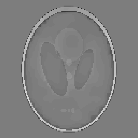
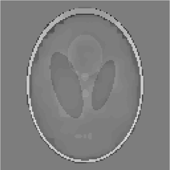
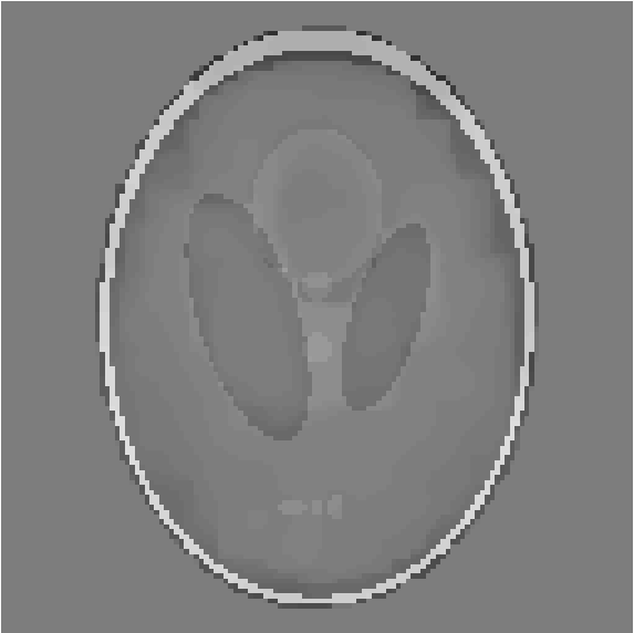
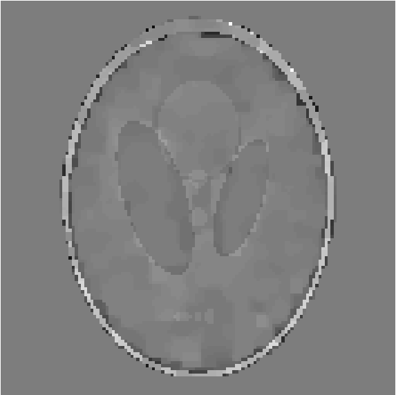
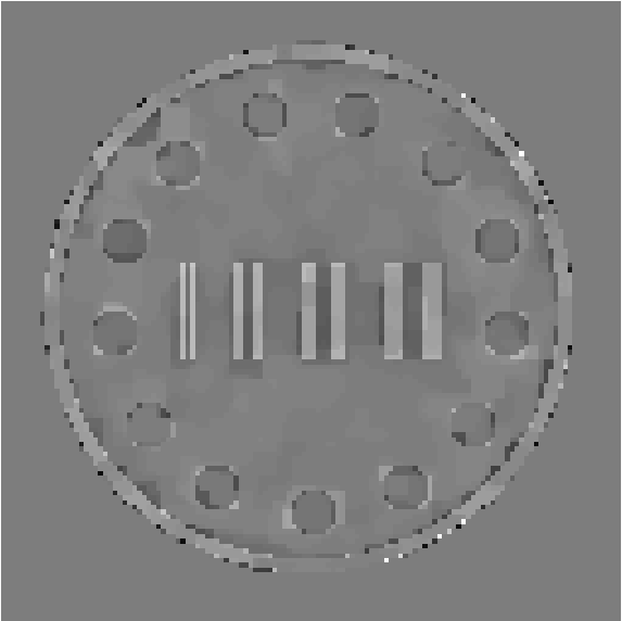
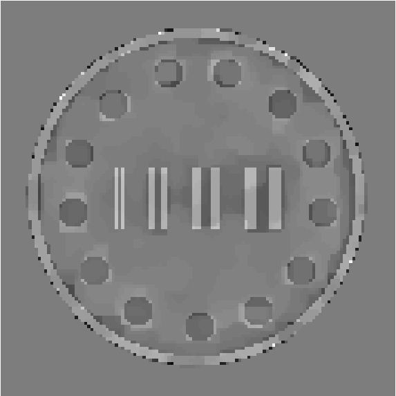
First, we take simulated data: the ground-truth images are Shepp-Logan and PET [15] phantoms of size ; The map is a discrete Radon transform, formed using MATLAB built-in function radon with projections per angle and three different angle settings, i.e., , and , and accordingly, the matrix is of size , and . For each image, we consider two count levels: the moderate count case is obtained from , and the low count case from (so that the measured counts are mostly below 10). The original image, sinogram and observed Poisson data are shown in Figs. 1 and 4 for Shepp-Logan and PET, respectively. The numerical results are summarized in Tables 2 and 3, Figs. 2–3 and Figs. 5–6. The EP mean is mostly comparable with MAP in all three metrics for both moderate count and low count cases, and the reconstruction quality improves steadily as the number of projection angles increases. Interestingly, the shape of the EP variance resembles closely the outer boundary of the phantom, whereas within the boundary, there is little difference in the magnitudes. This might indicate that the algorithm is rather certain in the cold regions where the error is close to zero and more uncertain about the region where the error is potentially larger. It is observed that the computational complexity of the EP grows with the amount of the data. This is attributed to the following fact: the number of sweeps is fixed at four, and the complexity increases with the number of projection angles. Since the computing time is presented only for one reconstruction at each case, these numbers should be viewed as a representative instead of an absolute measure for algorithmic performance. Roughly, EP is about two orders of magnitude more expensive than the MAP approach (computed by limited memory BFGS [31]).
The Poisson model is especially useful for low count data, where a naive Gaussian approximation can fail to give reasonable reconstructions. The EP results for the low-count case are shown in Figs. 3 and 6. Just as expected, the reconstruction accuracy deteriorates as the count level decreases. Nonetheless, the EP means remain largely comparable with MAP results both qualitatively and quantitatively. Note that for the PET image, the reconstruction accuracy for both EP and MAP suffers significantly in that the fine details such as vertical bars in the true image disappear, especially when the number of projection angles is small. The computing times for the moderate count and low count cases are nearly the same; see Tables 2 and 3. Thus, EP is still feasible for the low-count case.
| angle | [0:2:179] | [0:4:179] | [0:8:179] | |||
|---|---|---|---|---|---|---|
| 6e0 | 4e0 | 3e0 | ||||
| Method | EP | MAP | EP | MAP | EP | MAP |
| error | 5.32 | 5.36 | 5.64 | 5.67 | 6.09 | 6.11 |
| SSIM | 0.74 | 0.78 | 0.70 | 0.75 | 0.67 | 0.72 |
| PSNR | 18.58 | 18.53 | 17.97 | 17.93 | 17.29 | 17.27 |
| CPU time (s) | 80187.88 | 124.44 | 46031.95 | 55.55 | 29274.16 | 27.23 |
| 1.3e0 | 2e0 | 1e0 | ||||
| Method | EP | MAP | EP | MAP | EP | MAP |
| error | 4.07 | 4.09 | 6.15 | 6.24 | 6.14 | 6.19 |
| SSIM | 0.57 | 0.79 | 0.51 | 0.72 | 0.48 | 0.70 |
| PSNR | 19.50 | 19.47 | 17.53 | 17.42 | 17.18 | 17.15 |
| CPU time (s) | 82125.92 | 42.25 | 47110.50 | 29.69 | 29756.10 | 15.20 |
 |
  |
  |
  |
 |
| |
  |
  |
  |
 |
|
|
|
|
| |
|
[0:2:179] |
 |
 |
 |
 |
 |
|---|---|---|---|---|---|
|
[0:4:179] |
 |
 |
 |
 |
 |
|
[0:8:179] |
 |
 |
 |
 |
 |
| MAP | MAP error | EP mean | EP error | EP variance |
|
|
|
|
| |
|
[0:2:179] |
 |
 |
 |
 |
 |
|---|---|---|---|---|---|
|
[0:4:179] |
 |
 |
 |
 |
 |
|
[0:8:179] |
 |
 |
 |
 |
 |
| MAP | MAP error | EP mean | EP error | EP variance |
| angle | [0:2:179] | [0:4:179] | [0:8:179] | |||
|---|---|---|---|---|---|---|
| 1.6e0 | 1.4e0 | 1.2e0 | ||||
| Method | EP | MAP | EP | MAP | EP | MAP |
| error | 7.37 | 7.45 | 8.55 | 8.64 | 8.81 | 8.87 |
| SSIM | 0.72 | 0.81 | 0.61 | 0.75 | 0.57 | 0.70 |
| PSNR | 19.82 | 19.79 | 18.42 | 18.35 | 17.35 | 17.28 |
| CPU time (s) | 91263.00 | 110.05 | 53863.77 | 78.69 | 31537.05 | 28.20 |
| 1.2e0 | 9e-1 | 7.5e-1 | ||||
| Method | EP | MAP | EP | MAP | EP | MAP |
| error | 8.96 | 9.04 | 9.30 | 9.35 | 10.13 | 10.17 |
| SSIM | 0.55 | 0.72 | 0.49 | 0.67 | 0.43 | 0.62 |
| PSNR | 17.66 | 17.61 | 16.93 | 16.89 | 15.84 | 15.81 |
| CPU time (s) | 82542.76 | 52.97 | 47263.64 | 32.43 | 29737.91 | 18.01 |
 |
 |
| (a) Shepp-Logan | (b) PET |
To further illustrate the approximation, we plot in Fig. 7 the cross-sections and 95% highest posterior density (HDP) region, which is estimated from the EP covariance. The EP mean is close to MAP, and thus also suffers slightly from a reduced magnitude, as is typical of the total variation penalty in variational regularization [10]. This also concurs with the error metrics in Tables 2 and 3. The thrust of EP is that it can also provide uncertainty estimates via covariance, which is unavailable from MAP. In sharp contrast, the popular Laplace approximation (see Appendix B) can fail to yield a reasonable approximation for nonsmooth priors such as anisotropic total variation, whereas MCMC tends to be prohibitively expensive for large images, though being asympotically exact; see Appendix C for further numerical results. So overall, EP represents a computationally feasible approach to deliver uncertainty estimates for these benchmark images with Poisson data.
5.2 Convergence of the EP algorithm
Next, we present an experimental evaluation of the convergence of the EP algorithm, which is a long outstanding theoretical issue, on the following experimental setup: Shepp-Logan phantom and Radon matrix (i.e., projections per angle and , moderate count case). We denote the mean and covariance after outer iterations (i.e., sweeps through all the sites) by and , respectively, and the converged iterate tuple by . The EP mean converges rapidly, and visually it reaches convergence after five iterations since thereafter the cross-sections graphically overlap with each other; see Fig. 8. Thus, in the numerical experiments, we have fixed the number of outer iterations to four, and the complexity of the reconstruction algorithm is of order . Fig. 9 shows the errors of the iterate tuple with respect to , where the errors
are measured by the -norm and spectral norm, respectively. This phenomenon is also observed for all other experiments, although not presented. Hence, both mean and covariance converge rapidly, showing the steady and fast convergence of EP.
|
||||
 |
 |
 |
 |
 |
 |
 |
 |
 |
 |
 |
 |
| (a) mean | (b) covariance |
5.3 Real data
Last, we illustrate the inference procedure with a dataset taken from Michigan Image Reconstruction Toolbox11 1 https://web.eecs.umich.edu/~fessler/code/, last accessed on July 30, 2018.. The ground truth image is denoted by IRT. The map is assembled by , where is the system matrix and is an attenuation vector, by setting the mask to all values being unity and other parameters to default. The exact image and data are shown in Fig. 10; see Fig. 11 for reconstructions, obtained with a regularization parameter . The error, SSIM and PSNR for EP and MAP are, respectively, and , and , and and . Thus, the EP results and MAP are comparable, and the preceding observations remain valid.
  |
  |
 |
 |
 |
|
|
|
 |
 |
 |
 |
 |
| MAP | MAP error | EP mean | EP error | EP variance |
These numerical results with different experimental settings show clearly that EP can provide comparable point estimates with MAP as well as uncertainty information by means of the variance estimate.
6 Conclusion
In this work, we have developed inference procedures for the constrained Poisson likelihood arising in emission tomography. They are based on expectation propagation developed in the machine learning community. The detailed derivation of the algorithms, complexity and their stable implementation are given for a Laplace type prior. Extensive numerical experiments show that the EP algorithm (with natural parameters) converges rapidly and can deliver an approximate posterior distribution with the approximate mean comparable with MAP, together with uncertainty estimate, and can handle real images of medium size. Thus, the approach can be viewed as a feasible fast alternative to the general-purposed but expensive MCMC for rapid uncertainty quantification with Poisson data.
There are several avenues for future works. First, it is of enormous interest to analyze the convergence rate and accuracy of EP, and more general approximate inference techniques, e.g., variational Bayes, which have all achieved great practical successes but largely defied theoretical analysis. Second, it is important to further extend the flexibility of EP algorithms to more complex posterior distributions, e.g., lack of projection form. One notable example is isotropic total variation prior that appears frequently in practical imaging algorithms. This may require introducing an additional layer of approximation, e.g., in the spirit of iteratively reweighed least-squares or (quasi-)Monte Carlo computation of low-dimensional integrals. Third, many experimental studies show that EP converges very fast, with convergence reached within five sweeps for the Poisson model under considerations. However, the overall computational complexity per sweep of all current implementations [20] is still very high, and not scalable well to large images that are required in many real world applications. Hence, there remains great demand to further accelerate the algorithms, e.g., via low-rank structure of the map and diagonal dominance of the posterior covariance. Fourth and last, it is also important to derive rigorous error estimates for the quadrature rules developed in Section 4.
Appendix A Parameterizing Gaussian distributions
For a Gaussian with mean and covariance , the density is given by
where the parameters , and are respectively given by
Thus, the density is also uniquely defined by and . In the literature, is often referred to as the precision matrix and as the precision mean. and the pair is called the natural parameter of a Gaussian distribution.
It is easy to check that the product of Gaussians is also a Gaussian after normalization, and the mean and covariance of the product are given by
| (A.1) |
or equivalently
| (A.2) |
Appendix B Laplace approximation
In the engineering community, one popular approach to approximate the posterior distribution is Laplace approximation [43, 5]. It constructs a Gaussian approximation by the second-order Taylor expansion of the negative log-posterior around MAP . Upon ignoring the unimportant constant and smoothing the Laplace potential, the negative log-posterior is given by
| (B.1) |
where is a small smoothing parameter to restore the differentiability. The gradient and Hessian are given respectively by
Since , the Taylor expansion reads
| (B.2) |
and approximates the precision matrix. When , the second term in can be negligible and thus the Hessian of the negative log-likelihood is dominating; whereas for , the second term is dominating. In either case, the approximation is problematic. In practice, it is also popular to combine smoothing with an iterative weighted approximation (e.g., lagged diffusivity approximation [45]) by fixing in at , which leads to a modified Hessian:
The Hessians and will be close to each other, if are all small, which is expected to hold for truly sparse signals, i.e., for . One undesirable feature of Laplace approximation is that the precision approximation depends crucially on the smoothing parameter .
Appendix C Comparison with MCMC and Laplace approximation
Numerically, the accuracy of EP has found to be excellent in several studies [36, 19], although there is still no rigorous justification. We provide an experimental evaluation of its accuracy with Markov chain Monte Carlo (MCMC) and Laplace approximation. The true posterior distribution can be explored by MCMC [32, 37]. However, usually a large number of samples are required to obtain reliable statistics. Thus, to obtain further insights, we consider a one-dimensional problem, i.e., a Fredholm integral equation of the first kind [35] over the interval with the kernel and exact solution , where . It is discretized by a standard piecewise constant Galerkin method, and the resulting problem is of size , i.e., and . We implement a random walk Metropolis-Hastings sampler with Gaussian proposals, and optimize the step size so that the acceptance ratio is close to in order to ensure good convergence [7]. The hyperparameter in the prior distribution is set to . The chain is run for a length of , and the last samples are used for computing the mean and covariance.
To compare the Gaussian approximation by EP and MCMC results, we present the mean, MAP, covariance and HPD region. Both approximations concentrate in the same region, and the shape and magnitude of HPD / covariance are mostly comparable; see Figs. 12 and 13, showing the validity of EP. However, there are noticeable differences in the recovered mean: the EP mean is nearly piecewise constant, which differs from that by MCMC. So EP gives an intermediate approximation between the MAP and posterior mean. In comparison with MAP, EP provides not only a point estimate, but also the associated uncertainty, i.e., covariance. Interestingly, the covariance is clearly diagonal dominant, which suggests the use of a banded covariance or its Cholesky factor for potentially speeding up the algorithm.
 |
 |
| (a) EP mean and -HPD | (b) MCMC mean and -HPD |
 |
 |
 |
| (a) EP and MCMC means | (b) EP covariance | (c) MCMC covariance |
The Laplace approximation described in Appendix B depends heavily on the smoothing parameter , and clearly there is a tradeoff between accuracy of MAP and the variance approximation; see Fig. 14 for the numerical results corresponding to four different smooth parameters , based on the approximation (B.2). This tradeoff is largely attributed to the nonsmooth Laplace type prior, which pose significant challenges for constructing the approximation. Thus, it is tricky to derive a reasonable approximation to the target posterior distribution. In contrast, the EP algorithm only involves integrals, which are more amenable to non-differentiability, and thus can handle nonsmooth priors naturally.
 |
 |
 |
 |
| (a) | (b) | (c) | (d) |
In passing, we note that the uncertainty estimate from the posterior probability distribution differs greatly from the concept of noise variance [16], which is mainly concerned with the sensitivity of the reconstruction with respect to the noise in the input data . It is derived using chain rule and implicit function theorem, under the assumptions of good smoothness and local strong convexity of the associated functional [16]. In contrast, the uncertainty in the Bayesian framework as in this work originates from imprecise knowledge of the inverse solution encoded in the prior and the statistics of the data. Thus, the results of these two approaches are not directly comparable.
References
- [1] M. Abramowitz and I. A. Stegun. Handbook of Mathematical Functions: with Formulas, Graphs, and Mathematical Tables. Courier Corporation, 1965.
- [2] F. J. Anscombe. The transformation of Poisson, binomial and negative-binomial data. Biometrika, 35(3/4):246–254, 1948.
- [3] S. R. Arridge, K. Ito, B. Jin, and C. Zhang. Variational Gaussian approximation for Poisson data. Inverse Problems, 34(2):025005, 29 pp., 2018.
- [4] M. Bertero, P. Boccacci, G. Desiderà, and G. Vicidomini. Image deblurring with Poisson data: from cells to galaxies. Inverse Problems, 25(12):123006, 26 pp., 2009.
- [5] C. M. Bishop. Pattern Recognition and Machine Learning. Springer, New York, 2006.
- [6] D. M. Blei, A. Kucukelbir, and J. D. McAuliffe. Variational inference: a review for statisticians. J. Amer. Statist. Assoc., 112(518):859–877, 2017.
- [7] S. P. Brooks and A. Gelman. General methods for monitoring convergence of iterative simulations. J. Comput. Graph. Statist., 7(4):434–455, 1998.
- [8] A. C. Cameron and P. K. Trivedi. Regression Analysis of Count Data. Cambridge University Press, Cambridge, 2nd edition, 2013.
- [9] E. Challis and D. Barber. Gaussian Kullback-Leibler approximate inference. J. Mach. Learn. Res., 14:2239–2286, 2013.
- [10] T. F. Chan and J. Shen. Image Processing and Analysis. SIAM, Philadelphia, PA, 2005. Variational, PDE, Wavelet, and Stochastic Methods.
- [11] J. P. Cunningham, P. Hennig, and S. Lacoste-Julien. Gaussian probabilities and expectation propagation. Preprint, arXiv:1111.6832, 2011.
- [12] A. R. De Pierro. A modified expectation maximization algorithm for penalized likelihood estimation in emission tomography. IEEE Trans. Med. Imag., 14(1):132–137, 1995.
- [13] G. Dehaene and S. Barthelmé. Bounding errors of expectation-propagation. In C. Cortes, N. D. Lawrence, D. D. Lee, S. M., and R. Garnett, editors, Advances in Neural Information Processing Systems, volume 28, pages 244–252, 2015.
- [14] G. Dehaene and S. Barthelmé. Expectation propagation in the large data limit. J. R. Stat. Soc. Ser. B. Stat. Methodol., 80(1):199–217, 2018.
- [15] M. J. Ehrhardt, K. Thielemans, L. Pizarro, D. Atkinson, S. Ourselin, B. F. Hutton, and S. R. Arridge. Joint reconstruction of PET-MRI by exploiting structural similarity. Inverse Problems, 31(1):015001, 23 pp., 2015.
- [16] J. A. Fessler. Mean and variance of implicitly defined biased estimators (such as penalized maximum likelihood): applications to tomography. IEEE Trans. Imag. Proc., 5(3):493–506, 1996.
- [17] Y. Gal and Z. Ghahramani. Dropout as a Bayesian approximation: Representing model uncertainty in deep learning. In M. F. Balcan and K. Q. Weinberger, editors, Proc. Int. Conf. Mach. Learn., pages 1050–1059, 2016.
- [18] M. Gehre. Rapid Uncertainty Quantification for Nonlinear Inverse Problems. PhD thesis, University of Bremen, Bremen, 2013. https://d-nb.info/1072078589/34.
- [19] M. Gehre and B. Jin. Expectation propagation for nonlinear inverse problems–with an application to electrical impedance tomography. J. Comput. Phys., 259:513–535, 2014.
- [20] A. Gelman, A. Vehtari, P. Jylänki, C. Robert, N. Chopin, and J. P. Cunningham. Expectation propagation as a way of life. Preprint, arXiv:1412.4869, 2014.
- [21] G. H. Golub and C. F. Van Loan. Matrix Computations. John Hopkins University Press, Baltimore, 3rd edition, 2012.
- [22] T. Hohage and F. Werner. Inverse problems with Poisson data: statistical regularization theory, applications and algorithms. Inverse Problems, 32(9):093001, 56 pp., 2016.
- [23] K. Ito and B. Jin. Inverse Problems: Tikhonov Theory and Algorithms. World Scientific, Hackensack, NJ, 2015.
- [24] B. Jin. A variational Bayesian method to inverse problems with impulsive noise. J. Comput. Phys., 231(2):423–435, 2012.
- [25] B. Jin and J. Zou. Augmented Tikhonov regularization. Inverse Problems, 25(2):025001, 25 pp., 2009.
- [26] M. I. Jordan, Z. Ghahramani, T. S. Jaakkola, and L. K. Saul. An introduction to variational methods for graphical models. Mach. Learning, 37(2):183–233, 1999.
- [27] J. Kaipio and E. Somersalo. Statistical and Computational Inverse Problems. Springer-Verlag, New York, 2005.
- [28] Y.-J. Ko and M. W. Seeger. Expectation propagation for rectified linear poisson regression. In G. Holmes and T.-Y. Liu, editors, Asian Conference on Machine Learning, volume PMLR 45, pages 253–268, 2016.
- [29] S. Kullback and R. A. Leibler. On information and sufficiency. Ann. Math. Stat., 22:79–86, 1951.
- [30] H. Lim, Y. K. Dewaraja, and J. A. Fessler. A PET reconstruction formulation that enforces non-negativity in projection space for bias reduction in Y-90 imaging. Phys. Med. Biol., 63(3):035042, 14 pp., 2018.
- [31] D. C. Liu and J. Nocedal. On the limited memory BFGS method for large scale optimization. Math. Progr., Ser. B, 45(3):503–528, 1989.
- [32] J. S. Liu. Monte Carlo Strategies in Scientific Computing. Springer-Verlag, New York, 2001.
- [33] T. P. Minka. A Family of Algorithms for Approximate Bayesian Inference. PhD thesis, Massachusetts Institute of Technology, Cambridge, 2001.
- [34] T. P. Minka. Expectation propagation for approximate Bayesian inference. In J. S. Breesc and D. Koller, editors, Proc. 17th Conf. Uncertainty in Artificial Intelligence, pages 362–369, 2001.
- [35] D. L. Phillips. A technique for the numerical solution of certain integral equations of the first kind. J. Assoc. Comput. Mach., 9:84–97, 1962.
- [36] C. E. Rasmussen. Gaussian processes in machine learning. In O. Bousquet, U. von Luxburg, and G. Rätsch, editors, Advanced Lectures on Machine Learning, Lecture Note in Computer Science, Vol. 3176, pages 63–71. Springer, Heidelberg, 2004.
- [37] C. P. Robert and G. Casella. Monte Carlo Statistical Methods. Springer-Verlag, New York, second edition, 2004.
- [38] L. I. Rudin, S. Osher, and E. Fatemi. Nonlinear total variation based noise removal algorithms. Phys. D, 60(1-4):259–268, 1992.
- [39] M. W. Seeger. Bayesian inference and optimal design for the sparse linear model. J. Mach. Learn. Res., 9:759–813, 2008.
- [40] L. A. Shepp and Y. Vardi. Maximum likelihood reconstruction for emission tomography. IEEE Trans. Med. Imag., 1(2):113–122, 1982.
- [41] S. Sotthivirat and J. A. Fessler. Image recovery using partitioned-separable paraboloidal surrogate coordinate ascent algorithms. IEEE Trans. Imag. Proc., 11(3):306–317, 2002.
- [42] A. M. Stuart. Inverse problems: a Bayesian perspective. Acta Numer., 19:451–559, 2010.
- [43] L. Tierney and J. B. Kadane. Accurate approximations for posterior moments and marginal densities. J. Amer. Statist. Assoc., 81(393):82–86, 1986.
- [44] Y. Vardi, L. Shepp, and L. Kaufman. A statistical model for positron emission tomography. J. Amer. Stat. Assoc., 80(389):8–20, 1985.
- [45] C. R. Vogel and M. E. Oman. Iterative methods for total variation denoising. SIAM J. Sci. Comput., 17(1):227–238, 1996.
- [46] J. Wang and N. Zabaras. Hierarchical Bayesian models for inverse problems in heat conduction. Inverse Problems, 21(1):183–206, 2005.
- [47] M. Welling and Y. W. Teh. Bayesian learning via stochastic gradient Langevin dynamics. In Proceedings of the 28th International Conference on Machine Learning, pages 681–688, 2011.
- [48] C. Zhang, J. Butepage, H. Kjellstrom, and S. Mandt. Advances in variational inference. IEEE Trans. Pattern Aal. Mach. Intell., page in press, 2019.