Two-dimensional grain boundary networks: stochastic particle models and kinetic limits
Abstract
We study kinetic theories for isotropic, two-dimensional grain boundary networks which evolve by curvature flow. The number densities for -sided grains, , of area at time , are modeled by kinetic equations of the form . The velocity is given by the Mullins-von Neumann rule and the flux is determined by the topological transitions caused by the vanishing of grains and their edges. The foundations of such kinetic models are examined through simpler particle models for the evolution of grain size, as well as purely topological models for the evolution of trivalent maps. These models are used to characterize the parameter space for the flux . Several kinetic models in the literature, as well as a new kinetic model, are simulated and compared with direct numerical simulations of mean curvature flow on a network. Existence and uniqueness of mild solutions to the kinetic equations with continuous initial data is established.
1 Introduction
1.1 Two dimensional grain boundary networks
We propose a new class of kinetic and stochastic models to describe the statistics of an evolving cellular network. We focus on the evolution of an isotropic, two dimensional grain boundary network consisting of smooth arcs such that:
(i) the normal velocity of each arc is proportional to its curvature (curvature flow); (ii) edges (typically) meet at trivalent junctions at an angle of (the Herring boundary condition) [13]. Such a network of arcs decomposes the plane into a disjoint collection of grains, each of which have the topology of polygons. Condition (ii) expresses the equilibrium of line tensions at a junction.
An important aspect of grain boundary evolution is the celebrated von Neumann-Mullins relation [21, 19]: the area of a grain with sides (a topological -gon) changes linearly in time
| (1) |
where is a material constant depending on surface tension and grain mobility. Thus, the geometry of each grain does not affect its growth, all that matters is the topology. In this setting, the statistics of a network with many grains are naturally described by a set of number densities that count the number of -sided cells per unit area that have area at time .
We derive kinetic equations that describe the evolution of from a simpler stochastic particle system that includes a deterministic drift (as in equation 1) along with stochastic ‘switching’ rules between populations based on the geometry of grain boundary networks. This particle system is an instance of a Piecewise Deterministic Markov Process (PDMP). Several similar kinetic theories have been proposed in the literature (as discussed in Section 5) on the basis of ad hoc rules, or comparison with experiments. However, there appears to have been no prior attempt to characterize the set of all possible kinetic models that may be derived from similar foundations (the von Neumann-Mullins rule and assumptions on the topological changes that arise when grains or grain boundaries vanish); nor does there appear to have been a prior attempt to compare the predictions of kinetic models with direct numerical simulations of grain boundary evolution.
1.2 Outline
from the geometry of grain boundary networks, a well-posedness analysis of the limiting kinetic equtions, and simulations which compare several previous kinetic models. This article is organized into three inter-related, but loosely dependent parts:
- 1.
- 2.
- 3.
Simulation of stochastic particle models that correspond to both new and existing kinetic models, with comparison to direct numerical simulations of a level set method (Section 7).
In technical terms, the first part of this paper is most closely tied to fluid-limits in queuing theory and the theory of piecewise-deterministic Markov processes. It can be viewed as a demonstration of the utility of these methods for cellular networks. The stochastic process studied here, an -species PDMP model, is a general model for particles that drift on the positive real line and mutate between several species. An interesting feature of this model is the set of mutation times, which are caused by particles reaching the origin. From the perspective of maps on surfaces, this corresponds to a face or edge collapsing to a point, and immediately changing its topology to satisfy the Herring conditions. Each mutation, from predetermined model parameters, induces randomness on particle positions, and thus makes mutation times random. Understanding the behavior of the system as a whole largely depends on describing the cumulative number of mutations, a ‘natural clock’ for the system. The interplay between mutation and empirical particle densities was rigorously studied in [15] with a minimal example, where authors JK and GM viewed the problem as an instance of a diminishing urn, and provided exponential concentration inequalities for the convergence of the particle model to its hydrodynamic limit.
While the first part focuses on the evolution of area statistics, with topological restrictions arising only in the description of boundary fluxes, the second part of this paper is devoted to a study of the ‘topological skeleton’ of grain boundary evolution. The analysis of annihilation and creation of grains is examined using the theory of maps on compact surfaces. These ideas are used to define a Markov chain on the space of trivalent maps (trivalent map evolution). We do not explore such Markov chains in detail. Instead, we use trivalent map evolution to systematically derive parameters for the stochastic particle system model.
In the third part, we provide a numerical comparison between stochastic particle simulations and direct numerical simulations of grain boundary networks using a level set method [7]. The stochastic particle models described in Section 2 are general enough to include assumptions from previous kinetic models [10, 9, 8, 17]. We also consider a new assumption which takes the rate of topological changes due to edge deletion events to be proportional to the total grain number. Our models also allow us to incorporate information about first-neighbor correlations in networks.
2 The stochastic particle system and kinetic equations
In Section 2.1, we will describe a class of particle processes which are amenable for modelling the coarsening, growth, and mutation found in cellular coarsening. These processes are examples of piecewise deterministic Markov processes (PDMPs). Roughly, the theory of PDMPs augments the structure of jump Markov processes to include random jumps triggered by deterministic drift. It is shown in Appendix A that the particle system defined informally below generates a well-defined evolution which is a strong Markov process. In Section 2.2, we present kinetic limits for PDMP models and state a well-posedness theorem for this limit, whose proof is provided in Appendix B.
2.1 The finite particle model
We consider a system of particles at time distributed amongst species. Each particle is of the form where indexes the species and denotes the size of the particle. The total number of particles in each species is denoted , thus . The letter (without the argument ) is always used to mean , and is a measure of the size of the system. The state of the system is denoted
| (2) |
The evolution of the system consists of a deterministic flow interspersed with stochastic jumps. We describe these in turn.
The deterministic flow is motivated by the von Neumann-Mullins rule. We divide the species into three distinct groups , and of size , and respectively, with . It is convenient to label these species in order:
| (3) | ||||
| (4) | ||||
| (5) |
For each species , we assume given a constant velocity , so that a particle of size at has size at time . The exit time for the particle is the time at which the size of the particle vanishes, namely
| (6) |
We assume that the species do not drift. That is, for . Finally, we assume for . The exit time for all particles of species and is .
Randomness is introduced into the system in the following way. As increases, each particle in the system drifts deterministically where is the flow map defined by for . Particles evolve until one of the following critical events occur:
- (B)
Boundary event: A particle hits the origin, i.e. for some with and .
- (I)
Interior event: An independent Poisson clock with rate attached to each particle rings.
To fix ideas, we illustrate these definitions in the context of grain boundary networks. Here the state of the system is a collection of grains, each belonging to one of topological classes; denotes the number of sides of a grain and denotes its area. The velocity field governing the evolution of an -gon is given by the von Neumann-Mullins rule 1. The critical events correspond respectively to: (B) the removal of a grain from the network when its size shrinks to zero; and (I) a random interchange of grains of different topology when an edge vanishes.
Though the size of each particle evolves deterministically, each boundary and interior event gives rise to a random mutation of particles of different species. We model each mutation with a mutation matrix. There are such matrices: matrices corresponding to the possible boundary events at each species , and one matrix for interior events. We find it necessary to include mutations in such generality to account for the topology of cellular networks – the topological changes arising from the vanishing of , and sided grains in grain boundary networks is not the same. Aside from some notational complexity, such generality does not affect the analysis. In Section 3, we explain how to choose the mutation rules based on the geometry of planar grain boundary networks.
Consider the boundary event when a single particle of species hits the origin. The corresponding mutation is determined by a positive integer , an mutation matrix taking values in , and a fixed -vector with positive entries. We choose particles and mutate them as follows. First, iid integers that index species are chosen with probability proportional to the weights and the total population of each species:
| (7) |
Second, for each random species , a random size is chosen with equal probability amongst the sizes of all the particles of species . Finally, these random particles are mutated as follows:
| (8) |
Thus, a particle of species with size is lost, and a particle of species with the size is created in the mutation. A particle of species with size 0 is also lost, so that the total number of the system decrements by one. Note that selection probabilities and mutations may vary for each of the mutating particles. See Figure 1 for an example with four species. In the degenerate event that the sizes of species, , hit the origin simultaneously, we repeat the process above times, ordering the boundary events at species in the sequence to be definite. Such ‘collisions’ occur with zero probability in the kinetic limit.
The process of mutation at an interior event is similar. No particle vanishes, but particles are mutated according to a fixed positive integer , a mutation matrix and weight as above. The integers are chosen with probability
| (9) |
and the particles mutated as follows
| (10) |
In the context of grain boundary coarsening, the necessity of introducing randomness for selecting grains results from a mean field assumption. Specifically, our models will track individual grain areas and number of sides, but not information about which grains neighbor each other. To determine mutated grains at a critical event, we select randomly according to equations (7)-(10), which impose that grains with identical topologies have equal chances of being selected to mutate, regardless of their areas.
In order to keep track of the flux in and out of a species we define the (constant) matrices with integer entries
| (11) |
Here and index species in , indexes a species in , and the entry counts the total number of mutations from species to species when a particle of species hits the origin. Similarly, enumerates the total number of mutations from species to species at an interior event. We assume that there are no trivial mutations from a species to itself, i.e.,
| (12) |
Summing over all species we obtain the identities
| (13) |
However, we do not assume detailed balance of mutations between species. That is, in general,
| (14) |

2.2 Kinetic limits of finite particle model
Several kinetic equations arise as limits of Markovian particle models. We now apply this approach to the particle models of Section 2.1
For each state and species we define an empirical measure
| (15) |
The empirical measures are normalized by the fixed initial number , not . Thus, is in general not a probability measure for . In what follows, we will not be interested in a rigorous demonstration of the convergence of empirical measures to solutions of kinetic equations (see [14] for a compactness argument for the convergence of empirical measures to kinetic equations). Rather, we begin with the assumption that for each species the weak limit is deterministic and has a number density
| (16) |
With these densities, we give a formal argument for kinetic equations. In Appendix B, we show well-posedness for these kinetic models, along with some expected conservation properties for special instances related to grain-boundary coarsening.
In the continuum limit, we can define the total numbers of particles in ,
| (17) |
and the weighted fractions
| (18) |
Then for each species , the formal kinetic equations for the number density are
| (19) | |||||
| (20) | |||||
| (21) | |||||
| (22) | |||||
While perhaps cumbersome at first sight, equation 19 is easily understood as a formal hydrodynamic limit of the particle PDMP described in the previous section. The index denotes a fixed species under consideration. The left-hand side of 19 describes the advection of the number density under the constant velocity . The right-hand side describes the growth and loss of species due to fluxes into and out of species . The fluxes in equations 20 and 21 arise from interior and boundary events. In these equations, the index enumerates all possible boundary events, and the index enumerates all the species that could mutate to species . A boundary event for species gives rise to both birth and death terms in proportion to the rate and the weights . The weights and defined in equation 11 arise as we sum over all mutations that lead to the creation of particles of species of size when a particle of species hits the origin. Similarly, such particles may be lost when they are mutated. This occurs in proportion to the weight . The terms multiplied by the rate account for interior events.
The boundary values , for the outgoing species play a subtle role in the kinetic equation since they determine the rate of boundary events. In order to obtain well-posedness of the kinetic equations, we will assume that the number densities are continuous on so that there is no ambiguity in defining their boundary values. In contrast, the boundary value of the species do not affect the flux and we impose the boundary conditions
| (23) |
2.3 Well-posedness
The kinetic equations 19 admit mild solutions on a maximal interval of existence. In order to define mild solutions, we integrate 19 along characteristics for each species to obtain
| (24) |
Here we assume that , . Thus, formula 24 is well defined for all species with , i.e. for . For the species with we must use the boundary condition 23 and a priori the integral in time is defined only over the time domain . However, for convenience, we extend the formula 24 to include the domain by setting when . It is then clear that 24 agrees with the solution obtained from the method of characteristics and the boundary condition 23.
Let denote the space of continuous and integrable functions equipped with the norm
| (25) |
It is easy to check that is a Banach space. We also denote
| (26) |
We say that is positive if for each and each . When is positive, .
Definition 1.
Theorem 1.
Assume given positive , and for . Also assume is constant. There exists a (possibly infinite) time and a unique map with such that is a positive, mild solution to 19 on each interval with . Further, if .
3 Topological evolution of trivalent maps
In this section we characterize the admissible topological changes during grain boundary evolution on a compact surface . In Section 4, these changes will be incorporated into our PDMP model of grain boundary coarsening through the mutation matrix .
Recall that a map is a graph drawn on a surface. More precisely, a map is a graph embedded in a surface in such a manner that (i) all vertices are distinct; (ii) none of the edges intersect except at vertices; (iii) each face obtained by cutting the surface along its edges is homeomorphic to an open disk [16, Ch.1.3]. The topology of a grain boundary network on is that of a trivalent map on . We denote the set of maps by and the set of trivalent maps by .
The topology of a grain boundary network stays constant when the evolution is smooth, but jumps when a grain or grain boundary vanishes. Thus, the topology of the network is a map that is piecewise constant. We adopt the convention that is right continuous. At a jump at time , is obtained from by a surgery consisting of the contraction of a face or edge of to a vertex followed by the attachment of a new graph at . The topology of must be consistent with the face or edge of that was contracted, as well as the irreversibility condition that energy cannot increase. We show below that these restrictions imply that must be a planar rooted tree.
The remainder of this section is organized as follows. We first establish the topological restrictions on attachment in Theorem 2 below. This is followed by the definition of a Markov chain on that may be used to model the ‘topological skeleton’ of grain boundary evolution. Finally, we apply these topological restrictions to obtain the mutation matrices for grain boundary evolution, thus connecting the size-based kinetic theory of Section 2 to topological changes.
3.1 The topology of attachment
We will restrict our analysis of detachment and attachment to the situation where at most one face shrinks to zero size or at most one edge shrinks to zero length. When a -sided face, , of a trivalent map vanishes we obtain a map with a -valent vertex. In a similar manner, if a single edge in a trivalent map shrinks to zero length, we obtain a -vertex.
It is convenient to introduce some notation for this process. Given , let denote the set of maps that are obtained from by contracting a -sided face () or an edge to a single vertex. Thus, every vertex in is trivalent, except for possibly one distinguished vertex, denoted , which is -valent, . Let denote the edges in that are incident to .
The process of attachment is a mapping from to that involves ‘blowing-up’ the vertex into a map and attaching to by the edges . The possible choices for are constrained by the following criterion:
- (i)
is a map into the closed unit disk with vertices on the boundary . We denote these vertices in cyclic order on .
- (ii)
All vertices of in the interior of are trivalent.
- (iii)
All interior faces of (i.e. faces whose edges lie in the interior of ) have at least seven sides.
Condition (i) is the boundary condition necessary so that can be attached to to obtain a trivalent map on . The vertices are temporary placeholders that are deleted when we attach to ; their role is to ensure that can be connected to by the edges . The other two conditions are consequences of irreversibility. Condition (ii) says that vertices that are not trivalent cannot persist in grain boundary evolution. Condition (iii) says that it is impossible to nucleate grains with six or fewer sides since this would contradict the Mullins-von Neumann relation. These criteria sharply limit the possible choices of .
Theorem 2.
Suppose and satisfies the conditions listed above. Then is a tree.
Corollary 1.
When , , or respectively, there are , , or topologically distinct choices for as shown in Figure 2.

Proof of Theorem 2.
We may trivially extend to a map into . Suppose that has vertices, edges, and faces. The number since always has an exterior face in . Let denoted the vertices of which lie in the interior of . Similarly, let denote the number of edges of that are not adjacent to the vertices on the boundary of . Finally, let denote the faces of in the interior of . By condition (iii) all faces must contain have than six sides. We will show that no such faces can exist. This relies on an identity relating the number of edges and vertices in .
All vertices are trivalent and all boundary vertices have degree one. We sum over the degrees of vertices in to obtain
| (27) |
We can also compare and . Since each interior face has at least 7 edges and there are interior faces, we obtain
| (28) |
In order to bound the right hand side of (28) we rewrite
| (29) |
where means that is an edge of the face . For each edge the corresponding term in the sum is either , or . Let denote the number of edges that are adjacent to a face as well as the exterior face of . Equivalently, this is the number of terms in the sum which are . Then
| (30) |
We show that , which means
| (31) |
To this end, recall that the vertices are ordered cyclically. Therefore, between any two vertices and there exists a path of edges that connect and , and are also edges of the exterior face of . The sequence of edges
| (32) |
forms a nonintersecting circuit of length at least , with each edge in the circuit bordering exactly one face in . This shows and proves (31).
Proof of Corollary 1.
We have established that the graph is a tree embedded in the disk , with labeled vertices on the boundary, and trivalent vertices in the interior of . For , let denote this set and denote its size. By splitting the tree into descendants of a degree one vertex, a direct recursive calculation shows that
| (34) |
The trees of relevance to us are shown in Figure 2. ∎
The description of trees above is closely related the Catalan numbers (see [20] for a variety of examples). Specifically, using the recurrence (34) for , is the nd Catalan number.

3.2 Trivalent map evolution
Theorem 2 allows us to formulate a Markov chain model for the topological evolution during grain boundary coarsening on a compact surface . In order to completely describe a Markov chain, we need a countable state space and a matrix of transition probabilites for jumps between states. Our state space is , where denotes a special, cemetery state. The neighbors of each state are characterized as follows:
- 1.
Annihilation : As in Section 3.1, , denotes the maps that may be obtained by contracting an edge of or a -sided face of , , to obtain a map with a distinguished vertex .
- 2.
Creation: A tree is glued to at to obtain a trivalent map . The set of all such maps is denoted .
Any assignment of transition probabilities for each , determines a Markov chain. The cemetery state is included to deal with the possibility that is empty. In this case, and . We call any Markov chain of this form trivalent map evolution (TME).
A trivalent map must always have faces with fewer than six sides when or . We use Euler’s formula along with the identities and
| (35) |
to see that the average number of edges in a face is given by
| (36) |
When , and , so that there is always a face with fewer than six sides. When , and we may always find a face with fewer than six sides unless is a hexagonal tiling. For all other compact surfaces, the genus , , so that .
3.3 Topological restrictions on kinetic models
Kinetic models for grain boundary coarsening typically assume the following grain coarsening rules at topological transitions (see Figure 4):
- •
If , two neighboring grains will both lose two sides.
- •
If , three neighboring grains will each lose one side.
- •
If , two neighboring grains each lose one side, and two neighboring grains retain their topology.
- •
If , two neighbors each lose one sides, one neighboring grain gains one side and two neighboring grains retain their topologies.
- •
If an edge connecting vertices and vanishes, with and adjacent to four distinct grains, then two of these grains each lose one side and the other two grains each gain one side.

However, trivalent map evolution may not follow these rules (see Fig. 5). An extra condition on the maps must be imposed so that TME is consistent with kinetic theory. An additional hypothesis is required, which is that all faces with sides have distinct neighboring grains, and that an edge and its two vertices are adjacent to four distinct faces. Denote this space as . For these embeddings11 1 The space is a proper subspace of closed 2-cell embeddings, in which the closure of each face is homeomorphic to a closed disc., the following holds.
Corollary 2.
Suppose . For a face or edge selected in the annihilation step of TME, the topological change from to follows the grain coarsening rules.
Proof.
If , then the distinguished vertex arising from the annihilation step of TME will be of degree , and will furthermore border distinct faces. From Corollary 1, we can directly verify that the grain coarsening rules hold for all of the possible trees that we may glue in the creation step of TME. Note that the creation step for TME with four and five sided grains can result in different possible topologies, but in all cases either two grains lose one side for a vanishing four-sided grain, or two grains lose a side and one grain gains a side for a vanishing five-sided grain. ∎

4 Topological kinetic equations
The major motivation for the PDMP model is to create a particle system representation for mean field models in grain boundary coarsening. In this section and Section 6, we will assign values to each of the parameters defined in Section 2 to correspond with key coarsening properties. In this section we will assign weights and mutation matrices related to the topological requirements of the grain coarsening rules enumerated in Section 3. This allows us to write topological kinetic equations, which should be considered as the most general set of kinetic equations for describing topological networks which evolve by TME and respect the grain coarsening rules. In Section 6, we will consider other parameters associated with edge deletion and first neighbor correlations. The free parameter space is sufficiently flexible to incorporate the correlation and edge-deletion assumptions of several of the models described in Section 5.
We now assign parameters for the PDMP model that we will consider fixed for all of the simulations carried out in Section 7. As mentioned in Section 2, particles correspond to individual cells of a two-dimensional grain network. A particle’s species corresponds its number of sides, and its position corresponds to its area. The most immediate of these is setting species velocity of , which is exactly the von Neumann-Mullins relation in which we set material constant in (1) to . Since grains with more than 10 sides are quite rare, we also cap the maximum number of sides at . Our models do not consider one-sided grains, as they are relatively rare in actual metal networks (around .1%, see [11]). To keep the system closed, we forbid two-sided grains to lose edges, three-sided grains to lose two edges, and sided grains to gain an edge at a critical events.
We also assign values for parameters related to topological transitions in networks which remain in during their evolution. This includes , the number of grains affected by deletion events, and the mutation matrices , which specify transitions for each such grain. Values for are
| (37) |
and the mutation matrices are defined as
| (38) | ||||
| (39) | ||||
| (40) | ||||
| (41) | ||||
| (42) |
Recall the upper index in refers to the number of sides for the deleted grain, refers to the number of sides of a neighboring grain before undergoing topology reassignment, and is the index of the th reassignment. Refer to Fig. 4 for a pictorial description of the distribution of sides before and after grain and edge deletions. Note that to keep the particle system closed, we disallow mutations that create 1 and sided grains.
With these defined parameters, we now give a more explicit form of the limiting kinetic equations of (19) for models of grain boundary coarsening. Assuming a continuous area density for -sided grains at time , we can write a system of topological kinetic equations for grains with sides as
| (43) |
for .
The four source terms of the right hand side of (43) describe, in order, addition and deletion of -sided grains due to grain deletions, and addition and deletion of -sided grains due to edge deletions. By directly substituting values of and into (19), we may write, for ,
| (44) | ||||
| (45) | ||||
| (46) | ||||
| (47) |
for tier weights and species selection weight fractions defined in (18).
5 Previous kinetic models
In this section, we review several previous kinetic models which describe area densities of -sided grains at time . All of the models assume that a neighbors are uncorrelated. Specifically, if we consider a single edge for some -sided grain, the probability that another grain with sides is its neighbor is , where is the total number of sides for all grains in the system. Three of the models mentioned here, those of Beenakker, Marder, and Flyvbjerg, assume no edge deletion.
5.0.1 The model of Beenakker
The model posed by Beenakker [3] begins by assuming grains are shaped like regular polygons, except having edges of circular arcs meeting at . This assumption gives the relation for an sided grain with area and perimeter where has an explicit (albeit lengthy) form. For distributions for -sided grains, an isotropic network in which thermal effects are neglected has a free energy given by the total perimeter
| (48) |
To obtain an equilibrium state, Beenakker minimizes over possible densities having with a fixed area and zero polyhedral defect, meaning
| (49) |
It can be shown that the minimizer for this variational problem gives a unique, explicit assignment of sides for all grains with area . Thus, densities take the form
| (50) |
From here, Beenakker invokes the rule to arrive at a simple evolution of area densities for time , given by
| (51) |
In a numerical integration of (51), Beenakker considers initial conditions of mostly hexagonal cells with a small fraction of pentagon-heptagon pairs. As expected, defects initially propagate in the system. However, a “collapse” eventually occurs in which the system rapidly returns to having near zero defect. The network then repeats this pattern indefinitely, oscillating between ordered and highly disordered states.
5.0.2 The model of Marder
Marder’s model [17] is unique in that it sets a rule for which neighbors lose an edge when a four-sided grain vanishes, choosing the two smallest grains. Similarly, when a five-sided grain vanishes, its two smallest neighbors lose an edge, and the largest neighbor gains an edge. The kinetic equations have the form
| (52) | ||||
| (53) |
Here and are the rates that -sided grains of area gain or lose a edge, respectively, and is the sum of all sides over all grains at time . Expressions for and are complicated, and involve probabilities that a grain selected at time has area greater than . A scaling analysis correctly shows that coarsening should be linear, and numerical approximations for (53) give statistics for topological frequency and coarsening that were comparable to experimental results on soap bubble networks.
5.0.3 The model of Flyvbjerg
Kinetic equations for Flyvbjerg’s model [8] are of the form
| (54) |
where tridiagonal coupling is given by
| (55) | ||||
| (56) | ||||
| (57) |
The transition rates for grains evolving from to sides contain boundary terms which make (54) nonlinear. An assumption for determining is that networks have zero first-neighbor correlations. This means that for any grain with sides, the probability that a neighboring grain has sides is independent of , and proportional to . To keep in a simplified form, Flyvbjerg assumptions required his model to allow for 1 and 0 sided grains. Simulations later showed these topologies were essentially negligible. In general, the comparison between Flyvbjerg’s model and experimental data is surprisingly accurate, with frequencies of topologies differing by only a few percentage points.
5.0.4 The model of Fradkov
The Fradkov model, posed in 1988 as a ‘gas approximation’ to grain coarsening [10, 9], has kinetic equations of the form
| (58) |
The collision operators , , account for topological transitions, taking the form
| (59) | ||||
| (60) |
Like the model of Flyvbjerg, topological transitions assume networks have zero correlation for first neighbors. Furthermore, collision operators also include a removal driven deletion assumption in which the ratio between edge deletion and grain deletion is a fixed constant . Thus, if denotes the total number of edge deletions under the Fradkov model, then
| (61) |
The quantity is then chosen to conserve total area, and invokes nonlinearity in the system. To keep the tridiagonal, topological effects from two-sided grains were ignored. The addition of an edge resulting from a five sided grain is also ignored. Derivations for both (59)-(60) and can be found in [12].
5.0.5 The BKLT model
The model of Barmak, Kinderlehrer, Livshits, and Ta’asan [2], or BKLT model, has topological coupling with the same general form as the right hand side of (54). In the absence of edge deletion, the coupling terms are determined through the conservation of polyhedral defect (49) to be
| (62) |
Here, is the rate of boundary deletion given by
| (63) |
and are free constants which satisfy . These constants are free, and can be fit through comparisons with experiments.
In [4], Cohen gives a stochastic description of the governing equations for the BKLT model in which a solution has an interpretation of a conditional backwards expectations of a sample tagged grain. We mention that in [4], Cohen considers the one-dimensional minimal model
| (64) |
as an explanatory example. In [15], two of this paper’s authors (JK and GM) considered (64) as a hydrodynamic limit of a one-species stochastic particle system on the positive real line, and proved exponential convergence of empirical densities to this limit.
6 Parameter fitting with direct numerical simulations
In order to complete the specification of our stochastic particle model,
it remains to provide expressions for the weights , which will represent topological frequencies of a grain’s neighbors, and the interior event intensity , which will represent the rate of edge deletion. For parameter fitting, the particle models will be compared with direct simulations of network flow, with data obtained from a level set method of Elsey, Esedoglu, and Smereka [6]. The numerical simulation is performed with 667,438 initial grains, determined from a Voronoi tesselation of the unit square with periodic boundary conditions. Grains evolve for a total time of , with updates given over two hundred uniform time steps (). The dataset from this simulation consists of each grain’s area and topology (included whether the grain vanished) over each time step.
6.1 First-neighbor correlations
From the species selection probabilities (7) and (9), the parameters allow us to weight the frequency of grains with sides which border grains with sides. Similar to the models of Flyvbjerg and Fradkov, we may assume frequencies are independent of the topology of the vanishing grain, and are only proportional to , meaning In this case, imposing again that grains have between 2 and sides, we obtain uncorrelated weights
| (65) | ||||||
| (66) | ||||||
| (67) | ||||||
Experiments on grain networks have shown that nontrivial nearest neighbor correlations do in fact exist, with grains having fewer sides tending to neighbor higher sided grains, and vice versa. The most popular relation is Aboav’s law [1], an empirical observation relating the average number of neighbors for an -sided cell as
| (68) |
where and are numerical constants. For our purposes, we are actually able to incorporate more information, and consider distributions which give the probability of a -sided cell to have a neighbor with sides, assuming the network to be stabilized. This distribution is not provided in the dataset provided from the level set used, so we instead use results in [18] which simulated grain boundary coarsening through a Monte Carlo-Potts model. With these distributions, we may estimate correlated weights from the level set simulation. This is done by using using topological frequencies simulated from the level set model which give the frequency of grains with sides. This is done at time , when about 80% of grains have vanished, and frequencies are essentially stable for the remainder of the simulation. Neighbor distributions for a -sided grain in the PDMP model may then be written in terms of and , and then compared with species selection probabilities to to obtain the linear system of equations in , given by
| (69) | ||||
| (70) |
Comparison between the weights and are given in Figure 6.

6.2 Edge deletion
6.2.1 Population-driven vs. removal-driven edge deletion
We now describe how to fit the rate function for several varieties of edge deletion models. The most simplified model, of course, is to assume no edge deletion at all. We may incorporate the no deletion assumption into the topological kinetic equations easily by setting , which we call the no edge deletion (ND) model.
Edge deletion for the topological kinetic equations at any fixed time is governed by a Poisson process with rate , where is the total number of grains at time . If we assume that is constant, then we call the resulting particle system a population-driven edge deletion (PD) model. We can fit by comparing against edge deletion rates in experimental data.
We may also consider a removal-driven edge deletion (RD) model motivated by Fradkov’s model [10, 9], which imposes that the total number of edge deletions is proportional to the total number of grain deletions. To derive such an expression of , we begin with an an explicit estimate for the total number . This estimate assumes a linear coarsening rate so that for a system with total area , the average grain size at time takes the form
| (71) |
This assumption, although not rigorously shown, is quite accurate in practice. Indeed, a linear regression on the coarsening rate for the level set data gives a Pearson correlation coefficient . With this assumption, the total number is
| (72) |
If denotes the total number of edge deletions under the RD model up to time , then
| (73) |
The quantity may be found by fitting against level set data. On the other hand, for the PD model, the total amount of edge deletion is
| (74) |
We equate with in (73) and (74), so that
| (75) |
Using (72), we may easily solve for in (75) to obtain the autonomous form
| (76) |
To summarize, in implementing the -species model, we obtain edge deletion similar to RD model assumptions by setting the rate of the Poisson clock to .
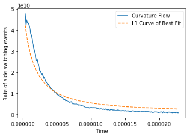
Fitted values for , and are given in Table 1. The coarsening rate was found through linear regression. The constant edge deletion rate was obtained by minimizing the distance over time between the rate of edge deletion and . Similarly, the Fradkov parameter was obtained by minimizing distance over time of the fraction of grains removed over edge deletions. See Figure 7 for graphs illustrating edge deletion behavior over time. Note that there appears to be a larger number edge deletions at the beginning of the simulation, possibly due to a burn-in period which adjusts to initial conditions of a Voronoi tessellation.
6.2.2 Estimating total edge deletion
We note here that tracking systems for grain networks in most level set methods, including the one used in this study, only track individual faces, and not edges. While we do not have precise data on edge deletion, we will present a method for estimating independent edge deletion using the level set dataset. This uses the available data of topologies and areas for each grain at each time step . The calculations for estimating total edge deletions are approximate for two reasons. First, we assume that each grain changes its number of sides at most once during a time step. Second, we ignore possible edge deletions occurring immediately before grain deletion, and thus assume that a grain changes its number of sides from either a vanishing neighboring grain, or an edge deletion from a neighboring grain of typical size.
To estimate total edge deletion, we record grains which vanish in the time interval . Under our assumptions, the total number of remaining grains which change their number of sides as a result of grain deletion is then
| (77) |
Let denote the total number of grains affected by both grain deletion and edge deletion. Since each edge deletion affects four neighboring grains, the total number of topological changes not due to grain deletions is then estimated as
| (78) |
7 Numerical results
In this section, we will simulate six varieties of PDMP models for coarsening, using either correlated or uncorrelated weights, and edge deletion rates assumptions that follow either the RD, PD, and ND models shown in Table 1. Each of these models are also compared with a level set method. For each model, 200,000 grains are sampled for initial conditions. Initial areas and topologies for the particle system model were selected through sampling with replacement from the initial empirical distribution of the level set model. After this selection, a small number of grains were then modified to produce a distribution with exactly 0 polyhedral defect, and like the level set simulation, evolve for a total time of .
| Model | ND | PD | RD |
|---|---|---|---|
| Switching | |||
| Fitted value | N/A |

Comparisons of grain statistics between the level set method and the three particle models are given in Figures 8-18 and Table 2. In Table 2, we use the total variation metric, which for two discrete probability vectors and is given by the distance
| (79) |
Distances between area distributions for grains with 5, 6, and 7 sides are measured with the Kolmogorov-Smirnov metric, which for two cumulative distribution functions is given by the distance
| (80) |
7.1 Topological frequencies of grains
Figures 8 and 9 show topological frequencies of grains with snapshots occurring at times for . Figure 10 shows topologies at , which corresponds to the time when approximately 20% of grains remain from the level set method, and also at all simulations’ end time of at which 31,887 grains remain from the level set method ( of initial grains).
For the level set model, topological frequencies stabilize quickly, with a minor trend for six sided grains to become less frequent, and five sided grains more frequent. Both the ND and RD models stabilize quickly, regardless of whether correlated weights are considered. Topological frequencies under the PD model with uncorrelated weights tend to become more uniform with time. Adding correlated weights, however, appears to reduce variance.
It has already been observed that higher rates of edge deletion are associated with more uniform distributions of grain topologies [10]. Thus, it is not surprising that the deletion-free ND model tends to concentrate near its mean of six sides more than the other models. For uncorrelated weights at , the ND and PD models differ from the level set method by a few percentage points, whereas the RD model is substantially more uniform. However, as frequencies under the PD model become more diffuse in time, as opposed to other models, by differences between the PD and level set models are magnified.
The addition of correlated weights appears to have two effects on topological frequencies. First, as noted before, diffusion is slowed under the PD model. Second, adding correlation for weights reduces variance. For the RD model, this reduces accuracy (see Table 2) against the level set model compared to the uncorrelated model, which already a smaller variance than the level set model. Adding correlation to the PD and RD model, however, increases accuracy, with the most drastic improvement occurring at .
7.2 Coarsening
In Figure 7, average grain area versus time is plotted for the level set and particle system model. For all models, coarsening rates appear to be linear, with almost no transition period from adjusting to initial conditions. The PD and RD models have similar coarsening weights, while the ND model coarsens significantly at a slower rate. Adding correlated weights has the effect of slowing coarsening, with all particle models having slower rates than the level set model.
7.3 Relative area distributions
Figures 11-18 provide snapshots of relative area densities for remaining grains at time . Relative area distributions were also considered in [2], but we also include relative areas of grains with 5, 6, and 7 sides. The Kolmogorov-Smirnov (KS) distances comparing particle models against the level set model are given in Table 2. For the level set method, area densities for 5, 6, and 7-sided grains have modes at positive values and tend to zero as areas approach zero. In contrast, densities for 5-sided grains for all particle models appear to be strictly decreasing. Positive modes appear for 6-sided grains, but densities for particle systems do not tend to zero as grain area approaches zero. Despite the similar shape of the level set and the ND model under both correlated and uncorrelated weights, the KS distance for 7-sided grains is larger than those of 5 and 6-sided grains. This is likely due to the sensitivity of the KS distance for distributions which are concentrated at a single value. We also note that expect for 5-sided grains under the PD and RD models, adding correlations increases the KS distance.
8 Conclusions
In this paper, we have developed a framework to study the coarsening of two dimensional isotropic grain boundary networks. The framework combines PDMP based particle systems, their kinetic limits, and a set of mutation rules based on topological restrictions. We show in Appendix B that the limiting kinetic equations for particle densities are well-posed in an appropriate Banach space. The parameters of the particle system can be varied to produce several models that describe grain boundary coarsening. All such models rely on mutation matrices which respect the topological changes during a grain or edge deletion. The remaining parameters, the selection weights and rates of interior events, may be chosen to satisfy other modeling assumptions related to first-neighbor correlations and edge deletion frequencies.
The results obtained from considering six separate particle models reveal that several types of qualitative behavior are dependent on the rate of edge deletion and first-neighbor correlations. As expected, increased edge deletion rates appear to increase the variance of the empirical distributions of one-point statistics of grain topologies. For the PD model, this smoothing is continuous in time, whereas in the RD and ND models, stabilization occurs almost immediately. With uncorrelated weights, the PD model remains similar to the level set model for some time, but eventually diverges as topological frequencies continue to smooth out. The addition of correlated weights appears to retard the variance of topologies for all models, and as a result, topological frequencies for the PD model perform substantially better when compared against the level set model. However, the improvement in statistics is not uniform across all of the metrics we consider. The uncorrelated PD and RD models, for instance, coarsen at a rate that is slower than the level set model. The addition of weights causes coarsening to slow, which in effect further decreases the accuracy of coarsening rates for the PD and RD models. Thus, it would be precipitate at this time to claim a specific particle model is superior.
To conclude, we find that the set of particle models offered in this paper are useful in several ways. Perhaps most importantly, they contain advantages of both the kinetic models developed in the past three decades and the accurate but computationally expensive direct simulation of grain networks. In particular, our model allows for rigorous examination of limiting densities. On the other hand, simulation of our model is relatively easy to implement compared to level-set methods. Implementation requires no discretization of differential equations, since advection of species occurs at constant rates, and mutation times are effectively handled with Poisson processes.


| Uncorrelated Weights | |||
|---|---|---|---|
| ND | PD | RD | |
| KS distance: 5 sides | .113 | .120 | .170 |
| KS distance: 6 sides | .262 | .247 | .322 |
| KS distance: 7 sides | .159 | .327 | .388 |
| KS distance: all grains | .064 | .147 | .156 |
| Total Variation () | .068 | .072 | .154 |
| Total Variation () | .069 | .232 | .177 |
| Correlated Weights | |||
| ND | PD | RD | |
| KS distance: 5 sides | .141 | .100 | .104 |
| KS distance: 6 sides | .304 | .301 | .369 |
| KS distance: 7 sides | .316 | .430 | .571 |
| KS distance: all grains | .235 | .262 | .226 |
| Total Variation () | .111 | .032 | .062 |
| Total Variation () | .114 | .124 | .072 |
9 Acknowledgements
This work was supported by NSF grants DMS 1714187 (JK), DMS 1344962 (GM), and DMS 1515400 and DMS 1812609 (RLP). GM acknowledges partial support from the Simons Foundation and the Charles Simonyi Fund at IAS. RLP was partially supported by the Simons Foundation and by the Center for Nonlinear Analysis under NSF PIRE Grant no. OISE-0967140.
10 Conflicts of Interest
The authors declare that they have no conflict of interest.
Appendix A Description of the -species system as a PDMP
We briefly review the basics of PDMPs, following Davis [5], and then explain how the -species stochastic particle process of Section 2.1 fits into this framework.
A.1 Background: General theory of PDMPs
We consider a countable set with elements denoted , a map , and open sets for each of the form . The state space is the disjoint union
| (81) |
The space has a natural topology. Let be the canonical injection defined by . A set is open if for every , is open in . The collection of all open sets may be used to define the set of Borel subsets of . This makes a Borel space.
A PDMP is an -valued generalized jump process , , that is prescribed by:
- 1.
Sufficiently smooth vector fields , .
- 2.
A measurable function .
- 3.
Points in travel according to flows defined by the vector fields until either a Poisson clock with intensity rings or the point hits the exit boundary . When such a critical event occurs the point jumps to a random new position whose law is given by .
Each vector field may be viewed as a first-order differential operator on . We assume they define a flow such that
| (82) |
for all sufficiently smooth test functions and for in a maximal interval of existence. The flow terminates only when hits
| (83) |
The exit boundary is the disjoint collection
| (84) |
At a given state we define the first exit time
| (85) |
and the survivor function
| (86) |
The stochastic process with initial condition is defined as follows. Choose a random time such that and an -valued random variable with law that is independent of . The trajectory of for is then
| (87) |
At , we repeat this process, replacing the jump time in the algorithm above with and the state with . Iterating this process, jump by jump, yields a cadlag process , .
Under modest assumptions, it can be shown that is a strong Markov process [5, §3]. We only require that is a measurable function of for each Borel set and a probability measure on for each . The rate function must be measurable with a little integrability: specifically, for each state we require the existence of such that the function is summable for . These conditions are easily verified in our model.
A.2 The -species model as a PDMP
We now show the -species model defined in Section 2.1 is a PDMP. Define the countable set of species indices
| (88) |
It is convenient to introduce notation that makes explicit the distinction between the number of particles in a state and the fixed parameter that is the normalizing factor in the empirical measure 15. We denote the number of particles in the state by and write
| (89) |
and the associated empirical measures is
| (90) |
For the -species process, , and equations 2,15 and equations 89–90are consistent.
Similarly, each open set and
| (91) |
The velocity fields on are obtained from the velocity fields , of the -species model,
| (92) |
and the exit boundary is
| (93) |
In order to define the transition kernel , we first describe the finite set of ‘neighbors’ for each state . Each point has a finite number, , of particles with size zero. Let us label these particles with indices ,,, , ordered such that the species . Let us begin by discussing the case when (this is the most important case, since boundary events happen at distinct times with probability ). When , the set may be decomposed into subsets, corresponding to boundary events at species. More precisely, a boundary event occurs at species , if the size and the associated species . According to the rules of Section 2.1, at such a boundary event, random variables are chosen, and mutated as in equation 8. Each such mutation gives rise to a neighbor of . Since the are a random collection of points of , we may write , for indices . Then is obtained from in two ‘sub-steps’:
- (i)
Pure mutation: is unchanged. The coordinates of are changed as follows: , . Call this intermediate state .
- (ii)
Removal of zero size: is changed to by deleting the particle with size zero.
The probability of each transition is given by the rules of Section 2.1. Finally, observe that these rules extend naturally to degenerate boundary points, where . In this case, according to the rules of Section 2.1, we order the points so that the species , and mutate and remove particles times in sequence as above.
Similarly, given an interior point we can use the mutation matrix and the weights to define a set of interior points that jumps to along with the corresponding probabilities . In this case, the transition involves only a mutation and no removal of zero sizes.
In summary, the transition kernel is given by
| (94) |
Since each particle carries an independent Poisson- clock , the first time that a clock rings follows the distribution . Thus
| (95) |
This completes the description of the -species model as a PDMP.
A.3 Conservation of total area and zero polyhedral defect
A benefit of using a finite particle system for grain boundary coarsening is the conservation of area and zero polyhedral defect. Using the notation presented above, we may write area of polyhedral defect in an particle system as function given by
| (96) |
Here, we used the identity function . Zero polyhedral defect for a trivalent planar network means that a grain has, on average, six sides, which follows from (36) for networks evolving on a torus.
Theorem 3.
For the PDMP model with fixed parameters from Sect. 4, suppose we have initial polyhedral defect and total area , for all times where the process is well-defined (i) and (ii)
Proof.
We consider a well-defined path for . In all realizations, this path will have a finite set of jump times .
To show conservation of zero polyhedral defect, suppose for a state that . We will directly show that defect does not change over jumps, or that
| (97) |
in the case of a three-sided grain vanishing (other critical events have similar proofs). Under a reindexing, we may write our state as
| (98) |
We may assume, without loss of generality, From (38)-(42) three particles with indices 2,3, and 4 lose an edge from The mutated state then takes the form
| (99) |
from which (97) follows immediately. This implies that . Since does not change between any jumps, if , then for all times in which the PDMP is well defined.
To show conservation of total area, again assume zero initial polyhedral defect. Then it is immediate that , and for for ,
| (100) |
∎
Appendix B Proof of well-posedness

Theorem 1 is proved in the following lemmas. The structure of the kinetic equations is a little more transparent when the flux is rewritten as a matrix vector product. Let and . We may then write
| (101) |
where the matrices and have off-diagonal terms given by
| (102) |
and diagonal terms given by
| (103) |
We first show that the flux , defined in 101, is a locally Lipschitz map. This allows us to obtain local existence of positive mild solutions by Picard’s method. We then extend the solutions to a maximal interval of existence by utilizing a more careful estimate of the flux.
Let denote the ball of radius centered at . As in 26 we denote
We adopt the following convention in the proof. The letter denotes a universal, positive, finite constant depending only on the parameters of the model such as the number of species , the constant velocities , the number of mutations and , the mutation matrices and , the weights and . It does not depend on .
Lemma 1 (Uniform bounds).
Assume is positive and non-zero. There exists , depending only on , such that for each .
| (104) |
Proof.
Recall that the flux is defined by equations 101–102. We will estimate each term in this expression in turn.
We first estimate . We find from 22 that for every
| (105) |
In order to estimate the weights defined by 18, we first establish a lower bound on the denominator for each . Let
We then have
| (106) | |||||
provided the radius satisfies
| (107) |
We assume that is chosen as above. It then follows from 102 and 103 that each entry in the matrix is bounded above by
| (108) |
Thus, the operator norm of the matrix satisfies the estimate22 2 , with , . Since is finite any norm may be chosen.
| (109) |
We combine 109 with 105 to see that the flux due to boundary events is bounded by
| (110) |
Lemma 2 (Lipschitz estimate).
Let and be as in Lemma 1. Then for every
| (113) |
Proof.
We use the expression 101 to obtain the inequality
| (114) | |||||
Let be fixed. It is clear that
| (115) |
For each , the difference is estimated as follows. Let and . Then
| (116) | |||||
using 106. It then follows from 102 and 103 that each term in the matrix satisfies an estimate as above, so that
| (117) |
Finally, we use the estimates 105, 109, 115 and 116 to obtain the Lipschitz bound:
A calculation similar to 111 yields the estimate
| (118) |
Thus, we find (also using the fact that is a constant)
| (119) |
∎
Lemma 3 (Local existence).
Assume is positive and non-zero. There exists a time and a map such that is the unique mild solution to 19 on the time interval that satisfies the initial condition .
Further, is positive for each .
Proof.
Lemma 4 (Maximal existence).
Let be a positive, mild solution. Then
| (123) |
There also exists a universal constant such that
| (124) |
where .
Equation 123 expresses conservation of the total number density of the system. The bound 124 degenerates if and only , i.e. if and only if for each , as approaches a critical time, say . It is well-known that continuous mild solutions on an interval can be uniquely continued onto a maximal interval of existence , such that . Thus, the above estimates suffice to complete the proof of Theorem 1.
Proof.
1. The conservation of number for the kinetic equations is a consequence of the switching rules for the particle system. We use the identity 13, and the definition of the fluxes in equations 20 and 21 to obtain the identity
| (125) |
It follows from 19 and 125 that
| (126) |
We integrate over to obtain the identity
| (127) |
The integral form of this identity is 123.
2. In order to prove 124 we combine equations 102 and 103 to obtain the pointwise estimate
| (128) |
Consequently, the flux due to boundary events satisfies the estimate
| (129) | ||||
| (130) |
From here, it is straightforward to obtain several regularity properties for mild solutions.
Theorem 4.
The following hold for mild solutions:
- 1.
Let denote the unique mild solution with initial condition for . Then, the map defined by is continuous in both time and space at all points where the map is well-defined.
- 2.
The maximum time of existence for mild solutions depends continuously on initial conditions.
- 3.
Let with . Then the mild solution is differentiable in both space and time for , and satisfies (19).
Proof.
We have already shown continuity in from a contraction mapping theorem. We now show continuous dependence on initial conditions. To show continuity in space, let with mild solutions and . For sufficiently close to , we may use (24) and (113) to show there exists such that for
,
| (134) |
An application of Gronwall’s inequality implies continuous dependence up to time . By a standard compactness argument, this may be extended to any with . This shows part (1), from which (2) follows immediately.
To prove (3), we show differentiability in space, using the (without loss of generality) right difference quotients
| (135) |
for . Similar to Part (1), through (24) and (113) we may show that for with , there exists a finite constant
| (136) |
Since , we may take to obtain The argument for time derivatives is identical.
∎
For the purposes of demonstrating global existence for PDMPs related to grain coarsening in Section B.1, we mention that characteristic speeds are bounded by .
Theorem 5 (Finite speed of propagation).
If has support contained in , then for , the support is contained in .
Proof.
B.1 Properties of kinetic equations for grain coarsening
B.1.1 Conserved quantities
Conservation of area and zero polyhedral defect for kinetic equations, defined similarly from (96), are conserved for the kinetic equations when considering initial data which is compactly supported.
Theorem 6.
Let . Then for ,
| (138) |
if and , then and for all .
Proof.
Suppose are differentiable with compact support for , and in as . By continuous dependence of parameters, for all , solutions in . Thus it is sufficient to show (138) for classical solutions. To do so, we integrate (43) and sum over all species to obtain
| (139) |
The left hand side of (139) is the polyhedral defect, and a straightforward computation using (44)-(47) shows that
| (140) |
which shows the conservation of polyhedral defect.
To show the conservation of area, we find through an integration by parts of (43) with (125) that
| (141) | ||||
| (142) |
For initial conditions with zero polyhedral defect, conservation of area then follows.
∎
The conservation of total area is sufficient to show global existence under a wide choice of weights.
Theorem 7 (Global existence).
Suppose , and , for For nonzero initial conditions with zero polyhedral defect, the maximum interval of existence for mild solutions is infinite.
Remark 1.
We require due to the impossibility of edge deletion in the pathological case of initial conditions , and for .
Proof.
Suppose for the sake of contradiction, that a finite maximum interval of existence . From Theorem 1, for some . We can check directly that from the conditions on , using zero polyhedral defect, that the stronger condition of must hold for all . Since from Theorem 5, there exists such that for and . This implies, however, that
| (143) |
a contradiction to the conservation of total area. ∎
References
- [1] Aboav, D.: The arrangement of grains in a polycrystal. Metallography 3(4), 383–390 (1970)
- [2] Barmak, K., Kinderlehrer, D., Livshits, I., Ta’asan, S.: Remarks on a multiscale approach to grain growth in polycrystals. In: Variational problems in materials science, pp. 1–11. Springer (2006)
- [3] Beenakker, C.: Evolution of two-dimensional soap-film networks. Physical review letters 57(19), 2454 (1986)
- [4] Cohen, A.: A stochastic approach to coarsening of cellular networks. Multiscale Modeling & Simulation 8(2), 463–480 (2010)
- [5] Davis, M.H.A.: Piecewise-deterministic Markov processes: a general class of nondiffusion stochastic models. J. Roy. Statist. Soc. Ser. B 46(3), 353–388 (1984). With discussion
- [6] Elsey, M., Esedoḡlu, S., Smereka, P.: Large-scale simulation of normal grain growth via diffusion-generated motion. Proceedings of the Royal Society A: Mathematical, Physical and Engineering Science 467(2126), 381–401 (2011)
- [7] Elsey, M., Smereka, P., et al.: Diffusion generated motion for grain growth in two and three dimensions. Journal of Computational Physics 228(21), 8015–8033 (2009)
- [8] Flyvbjerg, H.: Model for coarsening froths and foams. Physical Review E 47(6), 4037 (1993)
- [9] Fradkov, V., Glicksman, M., Palmer, M., Nordberg, J., Rajan, K.: Topological rearrangements during 2D normal grain growth. Physica D: Nonlinear Phenomena 66(1), 50–60 (1993)
- [10] Fradkov, V., Glicksman, M., Palmer, M., Rajan, K.: Topological events in two-dimensional grain growth: experiments and simulations. Acta Metallurgica et Materialia 42(8), 2719–2727 (1994)
- [11] Fradkov, V., Kravchenko, A., Shvindlerman, L.: Experimental investigation of normal grain growth in terms of area and topological class. Scripta metallurgica 19(11), 1291–1296 (1985)
- [12] Henseler, R., Herrmann, M., Niethammer, B., Velázquez, J.J.L.: A kinetic model for grain growth. Kinet. Relat. Models 1(4), 591–617 (2008). DOI 10.3934/krm.2008.1.591. URL http://dx.doi.org/10.3934/krm.2008.1.591
- [13] Herring, C.: Effect of change of scale on sintering phenomena. Journal of Applied Physics 21(4), 301–303 (2004)
- [14] Klobusicky, J.: Kinetic limits of piecewise deterministic markov processes and grain boundary coarsening. Ph.D. thesis, Brown University, Providence RI (2014)
- [15] Klobusicky, J., Menon, G.: Concentration inequalities for a removal-driven thinning process. Quarterly of Applied Mathematics 75(4), 677–696 (2017)
- [16] Lando, S.K., Zvonkin, A.K.: Graphs on surfaces and their applications, Encyclopaedia of Mathematical Sciences, vol. 141. Springer-Verlag, Berlin (2004). DOI 10.1007/978-3-540-38361-1. URL http://dx.doi.org/10.1007/978-3-540-38361-1. With an appendix by Don B. Zagier, Low-Dimensional Topology, II
- [17] Marder, M.: Soap-bubble growth. Physical Review A 36(1), 438 (1987)
- [18] Meng, L., Wang, H., Liu, G., Chen, Y.: Study on topological properties in two-dimensional grain networks via large-scale Monte Carlo simulation. Computational Materials Science 103, 165–169 (2015)
- [19] Mullins, W.: 2-Dimensional motion of idealized grain growth. Journal Applied Physics 27(8), 900–904 (1956)
- [20] Stanley, R.P.: Enumerative combinatorics. Vol. 2, Cambridge Studies in Advanced Mathematics, vol. 62. Cambridge University Press, Cambridge (1999). DOI 10.1017/CBO9780511609589. URL http://dx.doi.org/10.1017/CBO9780511609589. With a foreword by Gian-Carlo Rota and appendix 1 by Sergey Fomin
- [21] Von Neumann, J.: Discussion: grain shapes and other metallurgical applications of topology. Metal Interfaces (1952)