跳到论文正文
W Papers独立论文阅读器 arXiv:1810.07807 论文正文 计算阅读时间 · 0%
引用这篇论文根据当前论文元数据生成,正式投稿前建议核对。


License: arXiv.org perpetual non-exclusive license
arXiv:1810.07807v2 [cond-mat.stat-mech] 13 Jun 2019

Spontaneous symmetry breaking in 2D supersphere sigma models and applications to intersecting loop soups

Etienne Granet Affiliation: Institut de Physique Théorique, Paris Saclay, CEA, CNRS, 91191 Gif-sur-Yvette, France Affiliation: Laboratoire de Physique Théorique, Département de Physique de l’ENS, École Normale Supérieure, Sorbonne Université, CNRS, PSL Research University, 75005 Paris, France    Jesper Lykke Jacobsen Affiliation: Institut de Physique Théorique, Paris Saclay, CEA, CNRS, 91191 Gif-sur-Yvette, France Affiliation: Laboratoire de Physique Théorique, Département de Physique de l’ENS, École Normale Supérieure, Sorbonne Université, CNRS, PSL Research University, 75005 Paris, France Affiliation: Sorbonne Université, École Normale Supérieure, CNRS, Laboratoire de Physique Théorique (LPT ENS), 75005 Paris, France    Hubert Saleur Affiliation: Institut de Physique Théorique, Paris Saclay, CEA, CNRS, 91191 Gif-sur-Yvette, France Affiliation: USC Physics Department, Los Angeles CA 90089, USA
Abstract

Two-dimensional sigma models on superspheres Sr−1|2​s≅O​S​p​(r|2​s)/O​S​p​(r−1|2​s)S^{r-1|2s}\cong OSp(r|2s)/OSp(r-1|2s) are known to flow to weak coupling gσ→0g_{\sigma}\to 0 in the IR when r−2​s<2r-2s<2. Their long-distance properties are described by a free “Goldstone” conformal field theory (CFT) with r−1r-1 bosonic and 2​s2s fermionic degrees of freedom, where the O​S​p​(r|2​s)OSp(r|2s) symmetry is spontaneously broken. This behavior is made possible by the lack of unitarity.

The purpose of this paper is to study logarithmic corrections to the free theory at small but non-zero coupling gσg_{\sigma}. We do this in two ways. On the one hand, we perform perturbative calculations with the sigma model action, which are of special technical interest since the perturbed theory is logarithmic. On the other hand, we study an integrable lattice discretization of the sigma models provided by vertex models and spin chains with O​S​p​(r|2​s)OSp(r|2s) symmetry. Detailed analysis of the Bethe equations then confirms and completes the field theoretic calculations. Finally, we apply our results to physical properties of dense loop soups with crossings.

1 Introduction

The Mermin-Wagner theorem—which forbids spontaneous breaking of continuous symmetries in dimensions D≤2D\leq 2—relies in particular on the assumption of unitarity. It has long been known that when unitarity is broken—typically, in statistical mechanics systems where some “Boltzmann-weights” can be negative—stable massless Goldstone phases can indeed appear. A simple and beautiful example of this phenomenon is provided by 2D superspin models with orthosymplectic symmetry. These models involve “spins” with bosonic and fermionic components (more detail below), and enjoy symmetry under a supergroup, generalizing the usual orthogonal symmetry group to superspins. With rr bosonic and 2​s2s fermionic degrees of freedom, the symmetry is described by the orthosymplectic group O​S​p​(r|2​s)OSp(r|2s) which behaves, in many ways, like the ordinary group O⁡(N≡r−2​s)O(N\equiv r-2s). The spontaneously broken symmetry phase can be described by a sigma model with target space O​S​p​(r|2​s)/O​S​p​(r−1|2​s)≅Sr−1|2​sOSp(r|2s)/OSp(r-1|2s)\cong S^{r-1|2s}—a supersphere—and a single coupling constant, gσg_{\sigma}. The perturbative β\beta function to leading order is β=d​gσd​log⁡l∝(r−2​s−2)​gσ2\beta={dg_{\sigma}\over d\log l}\propto(r-2s-2)g_{\sigma}^{2}. For the physically relevant sign of positive gσg_{\sigma} and r−2​s>2r-2s>2 (which includes in particular the ordinary sphere sigma model), the flow is towards large coupling as usual: fluctuations grow at large distance, and the symmetry is eventually restored. Meanwhile, if r−2​s<2r-2s<2, the flow is towards weak coupling, and symmetry remains broken. In this case, the fixed point theory in the infra-red is a very simple Goldstone theory made of free massless scalars with r−1r-1 bosonic and 2​s2s fermionic components. It is a conformal field theory with central charge c=r−1−2​sc=r-1-2s and r−1r-1 non-compact directions.

Microscopic realizations of supersphere sigma models were proposed in [1] in terms of a loop soup where loops cover all the vertices of the square lattice, with every edge visited exactly once, every vertex visited exactly twice, and with possibility of crossing. Each crossing is given a special Boltzmann weight ww, which is the only parameter in the problem, apart from the loop weight, taken to be r−2​s≡Nr-2s\equiv N. Why this model provides a realization of the spontaneously broken O​S​p​(r|2​s)OSp(r|2s) symmetry phase was discussed in detail in [1]. In that reference, it was in particular checked numerically that the IR properties of the model are given by those of the Goldstone theory with central charge c=r−1−2​sc=r-1-2s indeed.

The lattice model of dense loops is expected to provide a physical realization of the broken symmetry phase for all finite, non-zero values of the coupling ww. Different values of ww correspond to different bare values of the coupling constant gσg_{\sigma}. Since the bare gσg_{\sigma} is usually finite, there will be logarithmic corrections to scaling, appearing for instance in powers of log⁡x\log x corrections to the pure conformal behavior expected in the fixed point Goldstone theory. The main goal of this paper is to study these corrections. This is interesting for several reasons. From a practical perspective, these corrections affect directly the correlations measured in dense loop models, which have a variety of interesting applications. From a more fundamental perspective, the dense loop model provides a regularization of the supersphere sigma model which is rather easy to study both analytically (via the Bethe-ansatz, see below) and numerically, since it involves lattice models with a small number of discrete, compact degrees of freedom. A lot of weak-coupling properties can then be investigated, which are much harder to get in ordinary sigma models such as O⁡(3)O(3) [2]. Finally, we recall that 2D sigma models on super-targets appear in a variety of contexts from string theory [3] to the study of phase transitions in non-interacting disordered 2D quantum electron gases [4, 5, 6] to the study of many statistical mechanics models [7, 8]. Our understanding of these models remains sketchy, largely because the loss of unitarity leads to unpleasant features, such as indecomposable action of the conformal symmetry [9].

The supersphere sigma models provide an interesting ground where to gain experience in these matters—here, for instance, by investigating perturbation of logarithmic conformal field theory.

Refer to caption
Refer to caption
Figure 1: A sample configuration of a dense loop soup where crossings are forbidden (left) or allowed (right). For clarity, each loop has been given a different color: these colors do not form part of the definition of the model.

Remarkably, there exists a series of integrable vertex models known to be in the universality class of the O​S​p​(r|2​s)OSp(r|2s) supersphere sigma models for r−2​s<2r-2s<2 [10, 11]. These models have edge degrees of freedom taking values in the O​S​p​(r|2​s)OSp(r|2s) fundamental representations, and are closely associated with special points in the phase diagram of the dense loop model [1]. In the limit of small spectral parameter, the transfer matrix of these vertex models gives rise to a spin chain Hamiltonian acting on the tensor product of r+2​sr+2s dimensional representations.

Our strategy in this paper will be to study the weak-coupling physics of the supersphere sigma models mostly by analyzing their integrable lattice regularizations using the Bethe ansatz technique. We will also compare these results with those of (logarithmic) conformal perturbation theory.

It is important to stress that integrable spin chains are not usually associated with free Goldstone theories such as the ones we will encounter below.11 1 Note in particular that for r>1r>1 the associated CFTs will have non-compact degrees of freedom, even though the spin chains have a finite number of states per site. The well known S​U​(2)SU(2) spin-12{1\over 2} chain for instance can be considered as a lattice regularization of the O⁡(3)O(3) sigma model but with topological angle θ=π\theta=\pi, and bare coupling of order unity [12],[13]. It flows to strong coupling in the IR, with long-distance conformal properties described by a level-one Wess-Zumino theory (thus with left and right S​U​(2)SU(2) current algebra symmetries). Here in contrast, the spin chains provide regularizations of sigma models with no topological term, small bare coupling constants, flowing to weak coupling in the IR, with long-distance properties described by free Goldstone CFTs where the O​S​pOSp symmetry is spontaneously broken.

The plan of the paper is as follows. We focus in the first section on O​S​p​(1|2)OSp(1|2), a case which has already been partly studied in [14]. We compute logarithmic corrections to the gaps directly from the σ\sigma-model Hamiltonian, and match them with the Bethe-ansatz results. Such a field theory calculation of the low-lying spectrum directly from the sigma model Hamiltonian, and its comparison to the spin chain discretization, has not been done before to our knowledge. The sigma model analysis involves perturbation of a logarithmic CFT, which we compare with a discussion by Cardy of logarithmic corrections in ordinary CFTs perturbed by marginal operators, and explain to which extent the results on perturbed CFTs apply to the logarithmic case. We then move on to study of the O​S​p​(r|2)OSp(r|2) chains with r=2,3,4r=2,3,4 in the following three sections with a similar approach. In the last section, we apply our results to the discussion of physical observables in dense loop soups and derive new predictions for the power-law and logarithmic decay of intersecting loops correlations. Some technical aspects are studied in the appendices. In particular, in Appendix C, we give formulas for logarithmic corrections directly from the Bethe ansatz equations, and study how these are perturbed when there is an additional source term at one site in the Bethe equations (that occurs in case of modified boundary conditions, or inclusions of strings).

We note that our work is not the first to address the topic of logarithmic corrections in orthosymplectic spin chains. In a previous paper [15] the logarithmic corrections for some states in the O​S​p​(3|2)OSp(3|2) chain (technically, those with spins j=1/2j=1/2, qq arbitrary, see below) were obtained numerically and interpreted as the value of the Casimir. A similar exercise was carried out in [16] for similar states and other O​S​p​(r|2​s)OSp(r|2s) models. Our paper extends and in some cases significantly corrects the results of these two references. It also provides analytical results from the Bethe-ansatz, as well as a detailed study of the relationship with the sigma models (including in particular a perturbative calculation of their properties) and the dense loop soups.

Before entering the subject, we briefly give a few definitions related to orthosymplectic spin chains.

1.1 Definitions/Reminders

1.1.1 The orthosymplectic symmetry

We give here a brief description of the orthosymplectic symmetry.

We first remind that the superspace ℝr|2​s\mathbb{R}^{r|2s} is parametrized by rr ’bosonic’ variables ϕ1,…,ϕr\phi_{1},...,\phi_{r} and 2​s2s ’fermionic’ variables η11,η12,…,ηs1​ηs2\eta^{1}_{1},\eta^{2}_{1},...,\eta^{1}_{s}\eta^{2}_{s} that satisfy [ϕi,ϕj]=0[\phi_{i},\phi_{j}]=0, [ϕi,ηlk]=0[\phi_{i},\eta^{k}_{l}]=0, {ηji,ηlk}=0\{\eta^{i}_{j},\eta^{k}_{l}\}=0. The scalar product between two vectors x,y∈ℝr|2​sx,y\in\mathbb{R}^{r|2s} is defined by

⟨x,y⟩=xt⋅Jr|2​s⋅y,\langle x,y\rangle=x^{t}\cdot J_{r|2s}\cdot y\,, (1)

where

Jr|2​s=(IrOr×2​sO2​s×rIs⊗J0|2),J0|2=(01−10),J_{r|2s}=\left(\begin{matrix}I_{r}&O_{r\times 2s}\\ O_{2s\times r}&I_{s}\otimes J_{0|2}\end{matrix}\right)\,,\quad J_{0|2}=\left(\begin{matrix}0&1\\ -1&0\end{matrix}\right)\,, (2)

with IrI_{r} the identity matrix of size r×rr\times r, and Oa×bO_{a\times b} the zero matrix of size a×ba\times b.

The group O​S​p​(r|2​s)OSp(r|2s) is the set of linear transformations on ℝr|2​s\mathbb{R}^{r|2s} that leave the norm invariant:

OSp(r|2s)={M∈ℳr+2​s,r+2​s,∀x∈ℝr|2​s,⟨x,Mx⟩=⟨x,x⟩}.OSp(r|2s)=\{M\in\mathcal{M}_{r+2s,r+2s}\,,\quad\forall x\in\mathbb{R}^{r|2s}\,,\langle x,Mx\rangle=\langle x,x\rangle\}\,. (3)

The Lie superalgebra o​s​p​(r|2​s)osp(r|2s) of such a group can be represented as [17]

o​s​p​(r|2​s)={(AXB−YEXtCYt−At);A,B,C∈ℳs,s;X∈ℳs,r;Y∈ℳr,s;E∈ℳr,r;Et=−E}.osp(r|2s)=\left\{\left(\begin{matrix}A&X&B\\ -Y&E&X^{t}\\ C&Y^{t}&-A^{t}\end{matrix}\right);A,B,C\in\mathcal{M}_{s,s};X\in\mathcal{M}_{s,r};Y\in\mathcal{M}_{r,s};E\in\mathcal{M}_{r,r};E^{t}=-E\right\}\,. (4)

In this representation the generators for o​s​p​(r|2)osp(r|2) will be denoted Jz,J+,J−J_{z},J_{+},J_{-}, F1,…,FrF_{1},...,F_{r}, G1,…,GrG_{1},...,G_{r}, Qi​jQ_{ij}, i,j=1,…,ri,j=1,...,r, i>ji>j and are such that

jz​Jz+j+​J++j−​J−+∑k=1r(fk​Fk+gk​Gk)+∑i>jqi​j​Qi​j=(jz/2f1...fnj+g10...qn​1f1..............gn−qn​1...0fnj−−g1...−gn−jz/2).j_{z}J_{z}+j_{+}J_{+}+j_{-}J_{-}+\sum_{k=1}^{r}(f_{k}F_{k}+g_{k}G_{k})+\sum_{i>j}q_{ij}Q_{ij}=\left(\begin{matrix}j_{z}/2&f_{1}&...&f_{n}&j_{+}\\ g_{1}&0&...&q_{n1}&f_{1}\\ ...&...&...&...&..\\ g_{n}&-q_{n1}&...&0&f_{n}\\ j_{-}&-g_{1}&...&-g_{n}&-j_{z}/2\\ \end{matrix}\right)\,. (5)

The commutation relations of the generators can be read off directly from this matrix representation. For example, for o​s​p​(1|2)osp(1|2) one has 55 generators Jz,J+,J−,F+,F−J_{z},J_{+},J_{-},F_{+},F_{-} that satisfy the following relations

[Jz,J±]=±J±,[J+,J−]=2​Jz\displaystyle[J_{z},J_{\pm}]=\pm J_{\pm}\,,\quad[J_{+},J_{-}]=2J_{z} (6)
[Jz,F1]=12​F1,[Jz,G1]=−12​G1,[J+,G1]=−F1,[J−,F1]=−G1\displaystyle[J_{z},F_{1}]=\frac{1}{2}F_{1}\,,\quad[J_{z},G_{1}]=-\frac{1}{2}G_{1}\,,\quad[J_{+},G_{1}]=-F_{1}\,,\quad[J_{-},F_{1}]=-G_{1}
{F1,F1}=2J+,{G1,G1}=−2J−,{F1,G1}=2Jz.\displaystyle\{F_{1},F_{1}\}=2J_{+}\,,\quad\{G_{1},G_{1}\}=-2J_{-}\,,\quad\{F_{1},G_{1}\}=2J_{z}\,.

As for the Casimir, we normalize it in such a way that it is the inverse of the Killing form of the generators (5) (i.e., the quadratic term in the eigenvalue jj of JzJ_{z} is 2​j22j^{2}). For example for o​s​p​(1|2)osp(1|2) it reads

𝒞=2​Jz2+(J+​J−+J−​J+)+12​(G1​F1−F1​G1).{\cal C}=2J_{z}^{2}+(J_{+}J_{-}+J_{-}J_{+})+\frac{1}{2}(G_{1}F_{1}-F_{1}G_{1})\,. (7)

The representation theory of the o​s​p​(r|2​s)osp(r|2s) algebras is a bit complicated, and involves (except when r=1r=1) issues of typicality. Rather than give generalities at this stage, we will recall necessary features in our case by case analysis below.

1.1.2 The supersphere σ\sigma-model

A simple but non-trivial field theory with O​S​p​(r|2​s)OSp(r|2s) symmetry is the theory of “free” fields constrained to lie on the supersphere of dimensions (r−1|2​s)(r-1|2s), i.e. the subset Sr−1|2​s⊂ℝr|2​sS^{r-1|2s}\subset\mathbb{R}^{r|2s} such that ∀x∈Sr−1|2​s,⟨x,x⟩=1\forall x\in S^{r-1|2s},\langle x,x\rangle=1. This is the non-linear σ\sigma-model with target space the supersphere Sr−1|2​sS^{r-1|2s}. We will restrict in the following to the case s=1s=1, and thus symmetries O​S​p​(r|2)OSp(r|2). The action is

S⁡(ϕ1,…,ϕr,η1,η2)=κ4​π​gσ​∫d​x​𝑑t​(∑i=1r∂μϕi​∂μϕi+2​∂μη2​∂μη1),S(\phi_{1},...,\phi_{r},\eta^{1},\eta^{2})=\frac{\kappa}{4\pi g_{\sigma}}\int dxdt\left(\sum_{i=1}^{r}\partial_{\mu}\phi_{i}\partial_{\mu}\phi_{i}+2\partial_{\mu}\eta^{2}\partial_{\mu}\eta^{1}\right)\,, (8)

with ∂μX​∂μX≡−(∂xX)2+(∂tX)2\partial_{\mu}X\partial_{\mu}X\equiv-(\partial_{x}X)^{2}+(\partial_{t}X)^{2}, and κ\kappa a normalization factor to make matching with existing literature easier.

The constraint then translates into

∑i=1rϕi2+2​η2​η1=1.\sum_{i=1}^{r}\phi_{i}^{2}+2\eta^{2}\eta^{1}=1\,. (9)

The model for r<4r<4 is known to flow to a Goldstone free theory. From integration of the leading order in the β\beta function d​gσd​log⁡L∝(r−2​s−2)​gσ2{dg_{\sigma}\over d\log L}\propto(r-2s-2)g_{\sigma}^{2} we find, after properly adjusting normalizations, replacing the RG scale by the size of the system, and setting g≡gσg\equiv g_{\sigma} for simplicity [18, 19]

g≈κ(4−r)​log⁡L/L0,for ​L→∞,g\approx\frac{\kappa}{(4-r)\log L/L_{0}}\,,\quad\mbox{for }L\to\infty\,, (10)

where L0L_{0} is, at the order we are working, an irrelevant length scale we shall take equal to unity in the following.

1.1.3 The orthosymplectic spin chain

We will study spin chains built from an RR-matrix that satisfies the Yang-Baxter equation and that belongs to the fundamental representation of the o​s​p​(r|2​s)osp(r|2s) superalgebra. Periodic boundary conditions will be considered in this paper, although the open boundary case is briefly addressed in appendix C.

Consider a spin chain on LL sites with periodic boundary conditions, each site ii being described by a ℤ2\mathbb{Z}_{2}-graded vector space ViV_{i} of dimension D=r+2​sD=r+2s. The Grassman parity pαp_{\alpha} of the α\alpha-th degree of freedom is defined as

pα\displaystyle p_{\alpha} =1if α=1,…,s or α=r+s+1,…,r+2s\displaystyle=1\quad\text{if }\alpha=1,...,s\quad\text{ or }\quad\alpha=r+s+1,...,r+2s (11)
=0if α=s+1,…,r+s.\displaystyle=0\quad\text{if }\alpha=s+1,...,r+s\,.

The Boltzmann weight of the chain is given by a matrix Ra​bR_{ab} that acts on the (graded) tensor product of two spaces Va×VbV_{a}\times V_{b}. It is thus a square matrix of size D2×D2D^{2}\times D^{2}. The transfer matrix t⁡(λ)t(\lambda) of the model at spectral parameter λ\lambda, that acts on the tensor product VL⊗…⊗V1V_{L}\otimes...\otimes V_{1} of LL spaces, is given by the supertrace of the monodromy matrix

t⁡(λ)\displaystyle t(\lambda) =∑i=1D(−1)pi​Ti​i​(λ)\displaystyle=\sum_{i=1}^{D}(-1)^{p_{i}}T_{ii}(\lambda) (12)
with T⁡(λ)\displaystyle\text{with }\quad T(\lambda) =Ra​L​(λ)​Ra​L−1​(λ)​…​Ra​1​(λ).\displaystyle=R_{aL}(\lambda)R_{aL-1}(\lambda)...R_{a1}(\lambda)\,.

Ti​j​(λ)T_{ij}(\lambda) denotes the (i,j)(i,j) component of TT in the auxiliary vector space VaV_{a}. The notation Ra​iR_{ai} means that RR acts on the whole tensor product Va⊗VL⊗…⊗V1V_{a}\otimes V_{L}\otimes...\otimes V_{1}, but non-trivially only on the spaces VaV_{a} and ViV_{i}. However the graded tensor product introduces signs everywhere, and for clarity we give the explicit expression of the components of the transfer matrix

t​(λ)β1​…​βLα1​…​αL=∑c1,…,cL=1DR​(λ)c1​βLαL​cL​R​(λ)cL​βL−1αL−1​cL−1​…​R​(λ)c2​β1α1​c1​(−1)pc1​(−1)∑j=2L(pαj+pβj)​∑i=1j−1pαi.\displaystyle t(\lambda)^{\alpha_{1}...\alpha_{L}}_{\beta_{1}...\beta_{L}}=\sum_{c_{1},...,c_{L}=1}^{D}R(\lambda)^{\alpha_{L}c_{L}}_{c_{1}\beta_{L}}R(\lambda)^{\alpha_{L-1}c_{L-1}}_{c_{L}\beta_{L-1}}...R(\lambda)^{\alpha_{1}c_{1}}_{c_{2}\beta_{1}}(-1)^{p_{c_{1}}}(-1)^{\sum_{j=2}^{L}(p_{\alpha_{j}}+p_{\beta_{j}})\sum_{i=1}^{j-1}p_{\alpha_{i}}}\,. (13)

Such an explicit expression can be found in [20].

Let us now choose a particular matrix RR. We impose the two following conditions

  1. (i)

    RR satisfies the graded Yang-Baxter equation

    R12​(λ)​R13​(λ+μ)​R23​(μ)=R23​(μ)​R13​(λ+μ)​R12​(λ),R_{12}(\lambda)R_{13}(\lambda+\mu)R_{23}(\mu)=R_{23}(\mu)R_{13}(\lambda+\mu)R_{12}(\lambda)\,, (14)
  2. (ii)

    RR has o​s​p​(r|2​s)osp(r|2s) symmetry: that is, for each generator AA of o​s​p​(r|2​s)osp(r|2s) (in a certain representation, not necessarily (5)), t⁡(λ)t(\lambda) commutes with Atot=∑i=1LAiA_{\rm tot}=\sum_{i=1}^{L}A_{i} where AiA_{i} acts on the vector space ViV_{i}.

We will write Ri​kl​jR_{ik}^{lj} the component along ej⊗ele_{j}\otimes e_{l} of the action of RR on ei⊗eke_{i}\otimes e_{k}, where the eie_{i}’s denote the basis vector of VV.

The following RR-matrix is known to satisfy these two properties [21]

Ra​b​(λ)=λ​Ia​b+Pa​b+2​λ2−r+2​s−2​λ​Ea​b,R_{ab}(\lambda)=\lambda I_{ab}+P_{ab}+\frac{2\lambda}{2-r+2s-2\lambda}E_{ab}\,, (15)

where Ia​bI_{ab} is the D2×D2D^{2}\times D^{2} identity matrix, Pa​bP_{ab} is the graded permutation operator

(I)i​kl​j=δi​j​δk​l,(P)i​kl​j=(−1)pi​pj​δi​l​δj​k,(I)^{lj}_{ik}=\delta_{ij}\delta_{kl}\,,\qquad(P)^{lj}_{ik}=(-1)^{p_{i}p_{j}}\delta_{il}\delta_{jk}\,, (16)

and Ea​bE_{ab} the matrix given by

(E)i​kl​j=(−1)i>r+s​(−1)j≤s​δi​k′​δj​l′,(E)^{lj}_{ik}=(-1)^{i>r+s}(-1)^{j\leq s}\delta_{ik^{\prime}}\delta_{jl^{\prime}}\,, (17)

with i′=D+1−ii^{\prime}=D+1-i, and (−1)x>y(-1)^{x>y} is −1-1 if x>yx>y, 11 if x≤yx\leq y. The Hamiltonian of the chain is then defined as

ℋ=dd​λlogt(λ)|λ=0.\mathcal{H}=\frac{d}{d\lambda}\log t(\lambda)\rvert_{\lambda=0}\,. (18)

The Yang-Baxter equation ensures that the transfer matrices t⁡(λ)t(\lambda) and t⁡(μ)t(\mu) at different spectral parameters commute, and it has been shown that the eigenvalues of tt can be determined with the Bethe ansatz [22, 23] (completeness is not proven; moreover some eigenvalues may be a bit singular, like the ground state of the o​s​p​(3|2)osp(3|2) spin chain for example that is obtained with coinciding Bethe roots that should be normally excluded) .

1.1.4 The critical exponents from the spin chain

If a model is described by a Conformal Field Theory (CFT) in the thermodynamic limit, then the content of the theory (central charge, conformal dimensions, structure constants; and in case of LCFT, the logarithmic couplings) can be seen from the finite-size corrections to the low-lying excited energies for large system sizes [24, 25, 26]. More precisely, denoting EL0E_{L}^{0} the energy of the ground state of a periodic chain, and eL0=EL0/Le_{L}^{0}=E_{L}^{0}/L its intensive form, one has

eL0=e∞−π​vF6​L2​c+o⁡(L−2),e_{L}^{0}=e_{\infty}-\frac{\pi v_{F}}{6L^{2}}c+o(L^{-2})\,, (19)

where e∞e_{\infty} is the thermodynamic value of the energy, cc is the central charge and vFv_{F} the Fermi velocity. The finite-size corrections to the energy of the excited states eLe_{L} contain the conformal dimensions h+h¯h+\bar{h} of the theory

eL−eL0=2​π​vFL2​(h+h¯)+o⁡(L−2),e_{L}-e_{L}^{0}=\frac{2\pi v_{F}}{L^{2}}(h+\bar{h})+o(L^{-2})\,, (20)

Some structure constants can be seen in the next-order finite-size corrections, see [26]. In case of logarithmic finite-size corrections

eL−eL0=2​π​vFL2​(h+h¯)+2​π​vFL2​log⁡L​α+o⁡(L−2​(log⁡L)−1),e_{L}-e_{L}^{0}=\frac{2\pi v_{F}}{L^{2}}(h+\bar{h})+\frac{2\pi v_{F}}{L^{2}\log L}\alpha+o(L^{-2}(\log L)^{-1})\,, (21)

the correlation functions of the field ϕ\phi associated to eLe_{L} are expected to satisfy at large xx

⟨ϕ⁡(x)​ϕ​(0)⟩∼1x2​(h+h¯)​(log⁡x)2​α,\langle\phi(x)\phi(0)\rangle\sim\frac{1}{x^{2(h+\bar{h})}(\log x)^{2\alpha}}\,, (22)

see [27] for a derivation.

In the following we will often refer to the quantity L22​π​vF​(eL−eL0){L^{2}\over 2\pi v_{F}}(e_{L}-e_{L}^{0}) as a “scaled gap”. We will also sometimes denote eL−eL0e_{L}-e_{L}^{0} by Δ​eL\Delta e_{L}.

2 O​S​p​(1|2)OSp(1|2)

2.1 The spectrum from field theory

We start by deriving the expected low-lying spectrum of the non-linear σ\sigma-model with O​S​p​(1|2)OSp(1|2) symmetry at first order in (log⁡L)−1(\log L)^{-1}.

2.1.1 General strategy

There is a common strategy for studying the different models. The first step is to derive the Hamiltonian in terms of the modes of the fields from the lagrangian. The expectation values of the Hamiltonian within modes are naively divergent: to regularize them, we express them in terms of their normal-ordered versions and isolate infinite sums. Every regularized value for these gives a Hamiltonian with the desired o​s​posp symmetry, and they have to be fixed by an additional condition. Once the expression of the states in term of the modes are derived, the eigenvalues of the Hamiltonian at order gg can then be obtained. This gives access to the logarithmic corrections by using (10).

2.1.2 The action

In the o​s​p​(1|2)osp(1|2) case the constraint (9) can be satisfied by imposing

ϕ1=1−η2​η1.\phi_{1}=1-\eta^{2}\eta^{1}\,. (23)

The action becomes then

S⁡(η1,η2)=κ2​π​g​∫d​x​𝑑t​(∂μη2​∂μη1−η1​η2​∂μη1​∂μη2).S(\eta^{1},\eta^{2})=\frac{\kappa}{2\pi g}\int dxdt(\partial_{\mu}\eta^{2}\partial_{\mu}\eta^{1}-\eta^{1}\eta^{2}\partial_{\mu}\eta^{1}\partial_{\mu}\eta^{2})\,. (24)

Upon the change of variable η1,2→g​η1,2\eta^{1,2}\to\sqrt{g}\eta^{1,2} it reads

S⁡(η1,η2)=κ2​π​∫d​x​𝑑t​(∂μη2​∂μη1−g​η1​η2​∂μη1​∂μη2).S(\eta^{1},\eta^{2})=\frac{\kappa}{2\pi}\int dxdt(\partial_{\mu}\eta^{2}\partial_{\mu}\eta^{1}-g\eta^{1}\eta^{2}\partial_{\mu}\eta^{1}\partial_{\mu}\eta^{2})\,. (25)

Here gg shall be treated at order 11. Recall that for large LL we have from (10)

g=κ3​log⁡L.g=\frac{\kappa}{3\log L}\,. (26)

2.1.3 The Hamiltonian

The first task is to derive the Hamiltonian corresponding to the action (25). For calculation convenience we write (25) as

S=κ2​π∫dxdt(−∂xη2∂xη1+η˙2η˙1+g𝒱(η1,η2)),S=\frac{\kappa}{2\pi}\int dxdt(-\partial_{x}\eta^{2}\partial_{x}\eta^{1}+\dot{\eta}^{2}\dot{\eta}^{1}+g\mathcal{V}(\eta^{1},\eta^{2}))\,, (27)

with 𝒱⁡(η1,η2)\mathcal{V}(\eta^{1},\eta^{2}) a generic potential. We take the system to be defined on a cylinder of unit radius, so that xx is integrated between 00 and 2​π2\pi, and tt between 00 and an arbitrary final time TT. The derivatives with respect to fermions are always considered from the right (this means for example that (d/d​η˙2)​(η˙2​η˙1)=−η˙1(d/d\dot{\eta}^{2})(\dot{\eta}^{2}\dot{\eta}^{1})=-\dot{\eta}^{1}). In terms of modes

η1,2​(x,t)=∑kηk1,2​(t)​ei​k​x,\eta^{1,2}(x,t)=\sum_{k}\eta^{1,2}_{k}(t)e^{ikx}\,, (28)

the action reads

S=κ∫dt(∑k−k2ηk2η−k1+η˙k2η˙−k1+gV)=∫dtℒ,S=\kappa\int dt\left(\sum_{k}-k^{2}\eta^{2}_{k}\eta^{1}_{-k}+\dot{\eta}^{2}_{k}\dot{\eta}^{1}_{-k}+gV\right)=\int dt\mathcal{L}\,, (29)

with ℒ\mathcal{L} the lagrangian density, and

V⁡(t)=12​π​∫d​x​𝒱​(x,t).V(t)=\frac{1}{2\pi}\int dx\mathcal{V}(x,t)\,. (30)

The conjugate momenta to ηk1\eta^{1}_{k} and ηk2\eta^{2}_{k} are

πk1=κ​η˙−k2+κ​g​d​Vd​η˙k1,πk2=−κ​η˙−k1+κ​g​d​Vd​η˙k2.\pi^{1}_{k}=\kappa\dot{\eta}^{2}_{-k}+\kappa g\frac{dV}{d\dot{\eta}^{1}_{k}},\quad\pi^{2}_{k}=-\kappa\dot{\eta}^{1}_{-k}+\kappa g\frac{dV}{d\dot{\eta}^{2}_{k}}\,. (31)

The quantization procedure imposes the following anticommutators at equal times at all orders in gg:

{ηk1,2,πp1,2}=i​δk,p.\{\eta^{1,2}_{k},\pi^{1,2}_{p}\}=i\delta_{k,p}\,. (32)

The corresponding Hamiltonian is then defined as

H=∑k(πk1​η˙k1−η˙k2​πk2)−ℒ.H=\sum_{k}(\pi^{1}_{k}\dot{\eta}^{1}_{k}-\dot{\eta}^{2}_{k}\pi^{2}_{k})-\mathcal{L}\,. (33)

It gives, neglecting terms of order O⁡(g2)O(g^{2}):

H=∑k(κ​k2​ηk2​η−k1+κ−1​πk2​π−k1)−κ​g​V+O⁡(g2).H=\sum_{k}(\kappa k^{2}\eta^{2}_{k}\eta^{1}_{-k}+\kappa^{-1}\pi^{2}_{k}\pi^{1}_{-k})-\kappa gV+O(g^{2})\,. (34)

We now use the following expression of the time derivative for a quantity XX

X˙=i⁡[H,X],\dot{X}=i[H,X]\,, (35)

and the relation valid for all (commuting or anticommuting) quantities aia_{i} and bb (n≥2n\geq 2)

[an​…​a1,b]=∑i=1n(−1)i−1​an​…​ai+1​{ai,b}​ai−1​…​a1,[a_{n}...a_{1},b]=\sum_{i=1}^{n}(-1)^{i-1}a_{n}...a_{i+1}\{a_{i},b\}a_{i-1}...a_{1}\,, (36)

to compute

η˙k1\displaystyle\dot{\eta}^{1}_{k} =−κ−1​π−k2+κ​g​d​Vd​πk1,η˙k2=κ−1​π−k1+κ​g​d​Vd​πk2\displaystyle=-\kappa^{-1}\pi^{2}_{-k}+\kappa g\frac{dV}{d\pi^{1}_{k}}\,,\qquad\dot{\eta}^{2}_{k}=\kappa^{-1}\pi^{1}_{-k}+\kappa g\frac{dV}{d\pi^{2}_{k}} (37)
π˙k1\displaystyle\dot{\pi}^{1}_{k} =−κk2η2−k+κgd​Vd​ηk1,π˙2k=κk2η1−k+κgd​Vd​ηk2.\displaystyle=-\kappa k^{2}\eta^{2}_{-k}+\kappa g\frac{dV}{d\eta^{1}_{k}}\,,\qquad\dot{\pi}^{2}_{k}=\kappa k^{2}\eta^{1}_{-k}+\kappa g\frac{dV}{d\eta^{2}_{k}}\,.

Now let us define the following charges

Jz\displaystyle J_{z} =∑kηk1​πk1−ηk2​πk22​i,J+=−∑kiη1kπ2k,J−=−∑kiη2kπ1k\displaystyle=\sum_{k}\frac{\eta^{1}_{k}\pi^{1}_{k}-\eta^{2}_{k}\pi^{2}_{k}}{2i}\,,\qquad J_{+}=-\sum_{k}i\eta^{1}_{k}\pi^{2}_{k}\,,\qquad J_{-}=-\sum_{k}i\eta^{2}_{k}\pi^{1}_{k} (38)
F1\displaystyle F_{1} =∑k+l+m=0π2−k(δl,0δm,0+gη1lη2m),G1=∑k+l+m=0π1−k(δl,0δm,0−gη2lη1m).\displaystyle=\sum_{k+l+m=0}\pi^{2}_{-k}(\delta_{l,0}\delta_{m,0}+g\eta^{1}_{l}\eta^{2}_{m})\,,\qquad G_{1}=\sum_{k+l+m=0}\pi^{1}_{-k}(\delta_{l,0}\delta_{m,0}-g\eta^{2}_{l}\eta^{1}_{m})\,.

Using (32) one can check that they satisfy the o​s​p​(1|2)osp(1|2) relations (6)—remember that before (25) we made the replacement η1,2→g​η1,2\eta^{1,2}\to\sqrt{g}\eta^{1,2}. With the formulas (37) one has:

∂tJz\displaystyle\partial_{t}J_{z} =∑kκ​g2​(d​Vd​πk1​πk1+ηk1​d​Vd​ηk1−ηk2​d​Vd​ηk2−d​Vd​πk2​πk2)\displaystyle=\sum_{k}\frac{\kappa g}{2}\left(\frac{dV}{d\pi^{1}_{k}}\pi^{1}_{k}+\eta^{1}_{k}\frac{dV}{d\eta^{1}_{k}}-\eta^{2}_{k}\frac{dV}{d\eta^{2}_{k}}-\frac{dV}{d\pi^{2}_{k}}\pi^{2}_{k}\right) (39)
∂tJ+\displaystyle\partial_{t}J_{+} =∑kκ​g​(d​Vd​πk1​πk2+ηk1​d​Vd​ηk2),∂tJ−=∑kκ​g​(d​Vd​πk2​πk1+ηk2​d​Vd​ηk1)\displaystyle=\sum_{k}\kappa g\left(\frac{dV}{d\pi^{1}_{k}}\pi^{2}_{k}+\eta^{1}_{k}\frac{dV}{d\eta^{2}_{k}}\right)\,,\qquad\partial_{t}J_{-}=\sum_{k}\kappa g\left(\frac{dV}{d\pi^{2}_{k}}\pi^{1}_{k}+\eta^{2}_{k}\frac{dV}{d\eta^{1}_{k}}\right)
∂tF1\displaystyle\partial_{t}F_{1} =∑k+l+m=0g⁡(κ​d​Vd​η02​δl,0​δm,0−κ​k​m​ηl1​ηm2​ηk1+κ−1​ηk1​π−l1​π−m2)\displaystyle=\sum_{k+l+m=0}g\left(\kappa\frac{dV}{d\eta^{2}_{0}}\delta_{l,0}\delta_{m,0}-\kappa km\eta^{1}_{l}\eta^{2}_{m}\eta^{1}_{k}+\kappa^{-1}\eta^{1}_{k}\pi^{1}_{-l}\pi^{2}_{-m}\right)
∂tG1\displaystyle\partial_{t}G_{1} =∑k+l+m=0g⁡(κ​d​Vd​η01​δl,0​δm,0+κ​k​m​ηl2​ηm2​ηk1−κ−1​ηk2​π−l1​π−m2),\displaystyle=\sum_{k+l+m=0}g\left(\kappa\frac{dV}{d\eta^{1}_{0}}\delta_{l,0}\delta_{m,0}+\kappa km\eta^{2}_{l}\eta^{2}_{m}\eta^{1}_{k}-\kappa^{-1}\eta^{2}_{k}\pi^{1}_{-l}\pi^{2}_{-m}\right)\,,

where the following relation has been used (it is an integration by part)

∑k+l+m=0k2η1kη1lη2m=∑k+l+m=0k(k−k−l−m)η1kη1lη2m=∑k+l+m=0−kmη1kη1lη2m.\displaystyle\sum_{k+l+m=0}k^{2}\eta^{1}_{k}\eta^{1}_{l}\eta^{2}_{m}=\sum_{k+l+m=0}k(k-k-l-m)\eta^{1}_{k}\eta^{1}_{l}\eta^{2}_{m}=\sum_{k+l+m=0}-km\eta^{1}_{k}\eta^{1}_{l}\eta^{2}_{m}\,. (40)

With the equations (39) it can be checked that the following potential implies the conservation of all these charges:

𝒱⁡(η1,η2)=η2​η1​∂xη2​∂xη1−η2​η1​∂tη2​∂tη1,\mathcal{V}(\eta^{1},\eta^{2})=\eta^{2}\eta^{1}\partial_{x}\eta^{2}\partial_{x}\eta^{1}-\eta^{2}\eta^{1}\partial_{t}\eta^{2}\partial_{t}\eta^{1}\,, (41)

or in terms of VV

V=∑k+l+m+n=0(−m​n​ηk2​ηl1​ηm2​ηn1+κ−2​ηk2​ηl1​π−m1​π−n2).V=\sum_{k+l+m+n=0}\left(-mn\eta^{2}_{k}\eta^{1}_{l}\eta^{2}_{m}\eta^{1}_{n}+\kappa^{-2}\eta^{2}_{k}\eta^{1}_{l}\pi^{1}_{-m}\pi^{2}_{-n}\right)\,. (42)

Define now the following modes for all kk

ψk1\displaystyle\psi^{1}_{k} =−ikη1kκ1/2−π2−kκ−1/22,ψk2=−ikη2kκ1/2+π1−kκ−1/22\displaystyle=\frac{-ik\eta^{1}_{k}\kappa^{1/2}-\pi^{2}_{-k}\kappa^{-1/2}}{\sqrt{2}},\quad\psi^{2}_{k}=\frac{-ik\eta^{2}_{k}\kappa^{1/2}+\pi^{1}_{-k}\kappa^{-1/2}}{\sqrt{2}} (43)
ψ¯k1\displaystyle\bar{\psi}^{1}_{k} =−ikη1−kκ1/2−π2kκ−1/22,ψ¯2k=−ikη2−kκ1/2+π1kκ−1/22.\displaystyle=\frac{-ik\eta^{1}_{-k}\kappa^{1/2}-\pi^{2}_{k}\kappa^{-1/2}}{\sqrt{2}},\quad\bar{\psi}^{2}_{k}=\frac{-ik\eta^{2}_{-k}\kappa^{1/2}+\pi^{1}_{k}\kappa^{-1/2}}{\sqrt{2}}\,.

They satisfy

{ψk1,ψp2}=k​δk+p,0,{ψ¯k1,ψ¯p2}=k​δk+p,0\{\psi^{1}_{k},\psi^{2}_{p}\}=k\delta_{k+p,0}\,,\qquad\{\bar{\psi}^{1}_{k},\bar{\psi}^{2}_{p}\}=k\delta_{k+p,0} (44)

for k,p≠0k,p\neq 0, the other anticommutators being zero. The original modes for k≠0k\neq 0 read in terms of the ψ\psi’s:

ηk1,2\displaystyle\eta^{1,2}_{k} =ik​2​κ​(ψk1,2−ψ¯−k1,2)\displaystyle=\frac{i}{k\sqrt{2\kappa}}(\psi^{1,2}_{k}-\bar{\psi}^{1,2}_{-k}) (45)
π−k1,2\displaystyle\pi^{1,2}_{-k} =±κ/2​(ψk2,1+ψ¯−k2,1).\displaystyle=\pm\sqrt{\kappa/2}(\psi^{2,1}_{k}+\bar{\psi}^{2,1}_{-k})\,.

The potential then reads

V=∑k+l+m+n=012​κ2​(−i​2​κ​η02+ψk2−ψ¯−k2k)​(−i​2​κ​η01+ψl1−ψ¯−l1l)​(ψm2​ψ¯−n1+ψ¯−m2​ψn1).V=\sum_{k+l+m+n=0}\frac{1}{2\kappa^{2}}\left(-i\sqrt{2\kappa}\eta^{2}_{0}+\frac{\psi^{2}_{k}-\bar{\psi}^{2}_{-k}}{k}\right)\left(-i\sqrt{2\kappa}\eta^{1}_{0}+\frac{\psi^{1}_{l}-\bar{\psi}^{1}_{-l}}{l}\right)(\psi^{2}_{m}\bar{\psi}^{1}_{-n}+\bar{\psi}^{2}_{-m}\psi^{1}_{n})\,. (46)

2.1.4 Normal order

Up to now no normal order has been put on the fields. The elementary annihilation operators are set to be the ψm1,2\psi^{1,2}_{m}, ψ¯m1,2\bar{\psi}^{1,2}_{m} with m≥0m\geq 0, and the elementary creation operators the same modes but for m<0m<0, as well as η01,2\eta^{1,2}_{0}. The normally ordered version of an operator XX is denoted :𝑋::\mathrel{X}: and is defined, for every product of elementary operators that appear in the expression of XX, by putting all the annihilation operators to the right of their creation operators, multiplied by the corresponding fermionic sign. Equivalently (this is much more convenient for practical purposes), it amounts to forbidding contractions between modes that compose the Hamiltonian. Indeed, the only difference between the Hamiltonian and its normally-ordered version is the contractions that appear whenever an annhilation operator is moved to the right of a creation operator. For example if one computes the expectation value

⟨0|ψ12(∑k:ψk2​ψ−k1:)ψ1−1|0⟩\displaystyle\langle 0|\psi_{1}^{2}\left(\sum_{k}:\mathrel{\psi^{2}_{k}\psi^{1}_{-k}}:\right)\psi^{1}_{-1}|0\rangle =⟨0|ψ12​(∑k<0ψk2​ψ−k1−∑k>0ψ−k1​ψk2+ψ02​ψ01)​ψ−11|0⟩\displaystyle=\langle 0|\psi_{1}^{2}\left(\sum_{k<0}\psi^{2}_{k}\psi^{1}_{-k}-\sum_{k>0}\psi^{1}_{-k}\psi^{2}_{k}+\psi^{2}_{0}\psi^{1}_{0}\right)\psi^{1}_{-1}|0\rangle (47)
=⟨0|ψ12​(−ψ−11​ψ12)​ψ−11|0⟩\displaystyle=\langle 0|\psi_{1}^{2}\left(-\psi^{1}_{-1}\psi^{2}_{1}\right)\psi^{1}_{-1}|0\rangle
=−1,\displaystyle=-1\,,

one actually contracts the ψ12\psi^{2}_{1} inside the Hamiltonian with the ψ−11\psi^{1}_{-1} outside the Hamiltonian, without touching the ψ−11\psi^{1}_{-1} inside the Hamiltonian (but counting the −- sign that comes when going through it).

The normal ordering is known to remove ’infinite quantities’ from the expression of the fields. These are actually sums of anticommutators {ηk1,πk1}=i\{\eta^{1}_{k},\pi^{1}_{k}\}=i. While no expectation value is taken, one may equally consider that {ηk1,πk1}=i⋅1|k|\{\eta^{1}_{k},\pi^{1}_{k}\}=i\cdot 1_{|k|} where 1k=1−k1_{k}=1_{-k} is a bosonic variable that commutes with everything, and that could be treated on the same footing as the fermionic variables η\eta’s. This way these ’infinite quantities’ are of the form ∑k>01k\sum_{k>0}1_{k} which are regular elements of the algebra we are using. The only point is then to define a vacuum expectation value for this element of the algebra. Let us define thus

ξ0=∑m>01m,ξ−1=∑m>01mm.\xi_{0}=\sum_{m>0}1_{m},\quad\xi_{-1}=\sum_{m>0}\frac{1_{m}}{m}\,. (48)

The bosonic charges are not altered by the normal order:

Jz\displaystyle J_{z} =:Jz:,J+=:J+:,J−=:J−:.\displaystyle=:\mathrel{J_{z}}:\,,\qquad J_{+}=:\mathrel{J_{+}}:\,,\qquad J_{-}=:\mathrel{J_{-}}:\,. (49)

However the fermionic charges change. With an implicit sum over k+l+m=0k+l+m=0 (that is explicitly written for mm in case of constraints), we have

F1\displaystyle F_{1} =π02+g​π−k2​ηl1​ηm2\displaystyle=\pi^{2}_{0}+g\pi^{2}_{-k}\eta^{1}_{l}\eta^{2}_{m} (50)
=π02+g​π−k2​η−k1​η02+i​g2​κ​π−k2​ηl1​(ψm2m−ψ¯−m2m)\displaystyle=\pi^{2}_{0}+g\pi^{2}_{-k}\eta^{1}_{-k}\eta^{2}_{0}+\frac{ig}{\sqrt{2\kappa}}\pi^{2}_{-k}\eta^{1}_{l}\left(\frac{\psi^{2}_{m}}{m}-\frac{\bar{\psi}^{2}_{-m}}{m}\right)
=:F1:−igη10+i​g2​κ(∑m<0[π2−kη1l,ψm2m]−∑m>0[π2−kη1l,ψ¯−m2m])\displaystyle=:\mathrel{F_{1}}:-ig\eta^{1}_{0}+\frac{ig}{\sqrt{2\kappa}}\left(\sum_{m<0}[\pi^{2}_{-k}\eta^{1}_{l},\tfrac{\psi^{2}_{m}}{m}]-\sum_{m>0}[\pi^{2}_{-k}\eta^{1}_{l},\tfrac{\bar{\psi}^{2}_{-m}}{m}]\right)
=:F1:−igη10−2​i​g2​κ∑m>0(im​2​κπ20+κ/2η10)1m\displaystyle=:\mathrel{F_{1}}:-ig\eta^{1}_{0}-\frac{2ig}{\sqrt{2\kappa}}\sum_{m>0}\left(\frac{i}{m\sqrt{2\kappa}}\pi^{2}_{0}+\sqrt{\kappa/2}\eta^{1}_{0}\right)1_{m}
=:F1:−igη10−igη10ξ0+gκ−1π20ξ−1.\displaystyle=:\mathrel{F_{1}}:-ig\eta^{1}_{0}-ig\eta^{1}_{0}\xi_{0}+g\kappa^{-1}\pi^{2}_{0}\xi_{-1}\,.

To go from the second line to the third line, we noticed that π−k2​ηl1\pi^{2}_{-k}\eta^{1}_{l} only involves ψ1,ψ¯1\psi^{1},\bar{\psi}^{1} that anticommute, so that the only ’ill-ordered’ case that can occur is when a creation operator ψm2,ψ¯m2\psi^{2}_{m},\bar{\psi}^{2}_{m} with m<0m<0 is at the right. Similarly:

G1=:G1:+igη20+igη20ξ0+gκ−1π10ξ−1.\displaystyle G_{1}=:\mathrel{G_{1}}:+ig\eta^{2}_{0}+ig\eta^{2}_{0}\xi_{0}+g\kappa^{-1}\pi^{1}_{0}\xi_{-1}\,. (51)

As for the potential, it reads with an implicit summation over k+l+m+n=0k+l+m+n=0

V\displaystyle V =−κ−1​ηk2​ηl1​(ψm2​ψ¯−n1+ψ¯−m2​ψn1)\displaystyle=-\kappa^{-1}\eta^{2}_{k}\eta^{1}_{l}(\psi^{2}_{m}\bar{\psi}^{1}_{-n}+\bar{\psi}^{2}_{-m}\psi^{1}_{n}) (52)
=:𝑉:−κ−1∑m<0n≤0[η2kη1l,ψ2m]ψ¯1−n+κ−1∑m≥0n>0[η2kη1l,ψ¯1−n]ψ2m−κ−1∑m<0n>0([η2kη1l,ψ2m]ψ¯1−n+ψ2m[η2kη1l,ψ¯1−n])\displaystyle=:\mathrel{V}:-\kappa^{-1}\sum_{\begin{subarray}{c}m<0\\ n\leq 0\end{subarray}}[\eta^{2}_{k}\eta^{1}_{l},\psi^{2}_{m}]\bar{\psi}^{1}_{-n}+\kappa^{-1}\sum_{\begin{subarray}{c}m\geq 0\\ n>0\end{subarray}}[\eta^{2}_{k}\eta^{1}_{l},\bar{\psi}^{1}_{-n}]\psi^{2}_{m}-\kappa^{-1}\sum_{\begin{subarray}{c}m<0\\ n>0\end{subarray}}\left([\eta^{2}_{k}\eta^{1}_{l},\psi^{2}_{m}]\bar{\psi}^{1}_{-n}+\psi^{2}_{m}[\eta^{2}_{k}\eta^{1}_{l},\bar{\psi}^{1}_{-n}]\right)
+κ−1∑n<0m≤0[η2kη1l,ψ1n]ψ¯2−m−κ−1∑n≥0m>0[η2kη1l,ψ¯2−m]ψ1n+κ−1∑n<0m>0([η2kη1l,ψ1n]ψ¯2−m+ψ1n[η2kη1l,ψ¯2−m])\displaystyle+\kappa^{-1}\sum_{\begin{subarray}{c}n<0\\ m\leq 0\end{subarray}}[\eta^{2}_{k}\eta^{1}_{l},\psi^{1}_{n}]\bar{\psi}^{2}_{-m}-\kappa^{-1}\sum_{\begin{subarray}{c}n\geq 0\\ m>0\end{subarray}}[\eta^{2}_{k}\eta^{1}_{l},\bar{\psi}^{2}_{-m}]\psi^{1}_{n}+\kappa^{-1}\sum_{\begin{subarray}{c}n<0\\ m>0\end{subarray}}\left([\eta^{2}_{k}\eta^{1}_{l},\psi^{1}_{n}]\bar{\psi}^{2}_{-m}+\psi^{1}_{n}[\eta^{2}_{k}\eta^{1}_{l},\bar{\psi}^{2}_{-m}]\right)
=:𝑉:−iκ​2​κ∑k∑m>0(η2kψ¯1k−η1−kψ2k−η1kψ¯2k+η2−kψ1k)1m\displaystyle=:\mathrel{V}:-\frac{i}{\kappa\sqrt{2\kappa}}\sum_{k}\sum_{m>0}(\eta^{2}_{k}\bar{\psi}^{1}_{k}-\eta^{1}_{-k}\psi^{2}_{k}-\eta^{1}_{k}\bar{\psi}^{2}_{k}+\eta^{2}_{-k}\psi^{1}_{k})1_{m}
=:𝑉:+iκ−2∑k(η2kπ2k+η1kπ1k)ξ0.\displaystyle=:\mathrel{V}:+i\kappa^{-2}\sum_{k}(\eta^{2}_{k}\pi^{2}_{k}+\eta^{1}_{k}\pi^{1}_{k})\xi_{0}\,.

Here, to get to the second line we had to treat separately the 6 different cases where at least one of the fields in (ψm2​ψ¯−n1+ψ¯−m2​ψn1)(\psi^{2}_{m}\bar{\psi}^{1}_{-n}+\bar{\psi}^{2}_{-m}\psi^{1}_{n}) is a creation operator. The ηk2​ηl1\eta^{2}_{k}\eta^{1}_{l} part is then already normally ordered, since the only possible ill-ordered case is when k=−lk=-l, but then the ordering of the ψ\psi part inside ηk2​ηl1\eta^{2}_{k}\eta^{1}_{l} for k>0k>0 cancels out with the ordering of the ψ¯\bar{\psi} part for k<0k<0.

The whole Hamiltonian is

H=\displaystyle H= ∑k<0(ψ2kψ1−k−ψ1kψ2−k+ψ¯2kψ¯1−k−ψ¯1kψ¯2−k)+2ψ20ψ10−c12−κg:𝑉:\displaystyle\sum_{k<0}(\psi^{2}_{k}\psi^{1}_{-k}-\psi^{1}_{k}\psi^{2}_{-k}+\bar{\psi}^{2}_{k}\bar{\psi}^{1}_{-k}-\bar{\psi}^{1}_{k}\bar{\psi}^{2}_{-k})+2\psi^{2}_{0}\psi^{1}_{0}-\frac{c}{12}-\kappa g:\mathrel{V}: (53)
−iκ−1g∑k(η2kπ2k+η1kπ1k)ξ0,\displaystyle-i\kappa^{-1}g\sum_{k}(\eta^{2}_{k}\pi^{2}_{k}+\eta^{1}_{k}\pi^{1}_{k})\xi_{0}\,,

with the central charge c=−2c=-2 obtained with a usual zeta regularization, namely assigning the value ζ(−1)=−1/12\zeta(-1)=-1/12 to the formal sum “∑k>0k\sum_{k>0}k” by analytically continuing the zeta function ζ⁡(x)=∑n>0n−x\zeta(x)=\sum_{n>0}n^{-x} to the negative axis. The normally ordered Hamiltonian corresponds to the first line. Although the total Hamiltonian commutes with the o​s​p​(1|2)osp(1|2) charges, this is not the case anymore when normal order is imposed. One thus has to work with the total Hamiltonian, taking into account the ξ\xi’s for which a prescription of expectation value has to be given. Note that any (complex) value of the ξ\xi’s preserves the commutation relations.

2.1.5 Building the states

Let us define the states on which we will compute expectation values. We define the conformal variables z=e−i​x+τz=e^{-ix+\tau} and z¯=ei​x+τ\bar{z}=e^{ix+\tau}with τ=i​t\tau=it. A state |ϕ⟩|\phi\rangle for a field ϕ⁡(x,t)\phi(x,t) is defined by

|ϕ⟩=ϕ⁡(z=0)​|0⟩.|\phi\rangle=\phi(z=0)|0\rangle\,. (54)

For example one has

|η1⟩=η01​|0⟩.|\eta^{1}\rangle=\eta^{1}_{0}|0\rangle\,. (55)

The derivatives with respect to zz such as |∂zη1⟩|\partial_{z}\eta^{1}\rangle deserve some comments. Because of the definition of the modes ψ\psi, we still have at all time

η1​(x,t)=∑kηk1​(t)​ei​k​x=η01+i​∑k≠0ψk1​(t)−ψ¯−k1​(t)k​2​κ​ei​k​x.\eta^{1}(x,t)=\sum_{k}\eta_{k}^{1}(t)e^{ikx}=\eta^{1}_{0}+i\sum_{k\neq 0}\frac{\psi^{1}_{k}(t)-\bar{\psi}^{1}_{-k}(t)}{k\sqrt{2\kappa}}e^{ikx}\,. (56)

Without interaction we simply have ψk1​(τ)=ψk1​(0)​e−k​τ\psi^{1}_{k}(\tau)=\psi^{1}_{k}(0)e^{-k\tau}. But with the interaction the time evolution of the ψ\psi’s is not trivial anymore, and involves a term of order gg with a product of three ψ\psi’s. The expression of η\eta in terms of z,z¯z,\bar{z}, and even more for ∂zη\partial_{z}\eta, is not valid anymore. In particular one cannot build the states as usual:

|∂zη1⟩≠−i​ψ−11​|0⟩,|\partial_{z}\eta^{1}\rangle\neq-i\psi^{1}_{-1}|0\rangle\,, (57)

contrary to the case g=0g=0. The left-hand side now involves a term of order gg. Precisely, using:

∂z=−12​iei​x−τ∂x+12ei​x−τ∂τ,\partial_{z}=-\frac{1}{2i}e^{ix-\tau}\partial_{x}+\frac{1}{2}e^{ix-\tau}\partial_{\tau}\,, (58)

we get

∂zη1​(x,τ)=−i2​κ​∑k(ψk1​(τ)+g​κ​κ2​d​Vd​πk1​(τ))​ei​x​(k+1)​e−τ.\partial_{z}\eta^{1}(x,\tau)=\frac{-i}{\sqrt{2\kappa}}\sum_{k}\left(\psi^{1}_{k}(\tau)+g\kappa\sqrt{\frac{\kappa}{2}}\frac{dV}{d\pi^{1}_{k}}(\tau)\right)e^{ix(k+1)}e^{-\tau}\,. (59)

Taking z=0z=0 selects k=−1k=-1 because of the factor ei​x​(k+1)e^{ix(k+1)}, hence

|∂zη1⟩=−i2​κ​ψ−11​|0⟩−i​κ​g2​d​Vd​π−11​|0⟩,|\partial_{z}\eta^{1}\rangle=\frac{-i}{\sqrt{2\kappa}}\psi^{1}_{-1}|0\rangle-i\frac{\kappa g}{2}\frac{dV}{d\pi^{1}_{-1}}|0\rangle\,, (60)

that is

|∂zη1⟩=−i⁡(1+g2​η02​η01)​ψ−11​|0⟩.|\partial_{z}\eta^{1}\rangle=-i(1+\frac{g}{2}\eta^{2}_{0}\eta^{1}_{0})\psi^{1}_{-1}|0\rangle\,. (61)

Remark moreover that one has indeed F1​(1+g2​η02​η01)​ψ−11​|0⟩=0F_{1}(1+\frac{g}{2}\eta^{2}_{0}\eta^{1}_{0})\psi^{1}_{-1}|0\rangle=0 and J+​(1+g2​η02​η01)​ψ−11​|0⟩=0J_{+}(1+\frac{g}{2}\eta^{2}_{0}\eta^{1}_{0})\psi^{1}_{-1}|0\rangle=0 and this state is indeed highest-weight.

However, if we look at terms involving a η\eta times a derivative, since we have

ηk1​d​Vd​π−k1=0,\eta^{1}_{k}\frac{dV}{d\pi^{1}_{-k}}=0\,, (62)

we do have

|η1​∂zη1⟩=−i​η01​ψ−11​|0⟩,|\eta^{1}\partial_{z}\eta^{1}\rangle=-i\eta^{1}_{0}\psi^{1}_{-1}|0\rangle\,, (63)

without any corrections in gg.

For terms such as |η1​∂zη1​…​∂zmη1⟩|\eta^{1}\partial_{z}\eta^{1}...\partial_{z}^{m}\eta^{1}\rangle the corresponding calculations happen to be not as easily tractable, but the state η01​ψ−11​…​ψ−m1\eta^{1}_{0}\psi^{1}_{-1}...\psi^{1}_{-m} is indeed annihilated by F1F_{1} (and J+J_{+}). Similarly, |∂zη1​…​∂zmη1⟩|\partial_{z}\eta^{1}...\partial_{z}^{m}\eta^{1}\rangle is not as easily computed, but (1+m​g2​η02​η01)​ψ−11​…​ψ−m1(1+m\frac{g}{2}\eta^{2}_{0}\eta^{1}_{0})\psi^{1}_{-1}...\psi^{1}_{-m} is annihilated by F1F_{1} and J+J_{+}.

2.1.6 Regularization

Any complex values for the ξ\xi’s give a Hamiltonian that commutes with the charges (that also depend on ξ\xi), and thus that has the o​s​p​(1|2)osp(1|2) symmetry and the classical non-linear sigma model as classical limit. However, since some of them appear in expectation values, one has to fix their value with an exterior argument. This is the only additional information that we need to quantize the model. Here we choose to fix the zero mode of the Hamiltonian. It reads

H0=−κ−1​(1−g​η01​η02)​π01​π02−κ−1​i​g​(η02​π02+η01​π01)​ξ0.H_{0}=-\kappa^{-1}(1-g\eta^{1}_{0}\eta^{2}_{0})\pi^{1}_{0}\pi^{2}_{0}-\kappa^{-1}ig(\eta^{2}_{0}\pi^{2}_{0}+\eta^{1}_{0}\pi^{1}_{0})\xi_{0}\,. (64)

This zero mode should give the Laplace-Casimir operator of the algebra, see [28], thus be proportional to (1−g​η01​η02)​π01​π02−i​g​(η02​π02+η01​π01)(1-g\eta^{1}_{0}\eta^{2}_{0})\pi^{1}_{0}\pi^{2}_{0}-ig(\eta^{2}_{0}\pi^{2}_{0}+\eta^{1}_{0}\pi^{1}_{0}). Hence we impose the value

⟨0|ξ0|0⟩=−1.\langle 0|\xi_{0}|0\rangle=-1\,. (65)

As for the value of ⟨0|ξ−1|0⟩\langle 0|\xi_{-1}|0\rangle, it does not enter the Hamiltonian nor the construction of the states, and thus has no influence on any expectation values.

Equivalently we could impose that the fermionic charges (and the bosonic ones) are not modified by the normal order. This constrains ξ0\xi_{0} to take the value −1-1 and ξ−1\xi_{-1} the value 00.

2.1.7 Correction to the energy levels

To evaluate the corrections at order gg to the energy levels, one has to compute the matrix elements ⟨ϕ1|H|ϕ2⟩\langle\phi_{1}|H|\phi_{2}\rangle where ϕ1\phi_{1} and ϕ2\phi_{2} are eigenstates of the unperturbed HH with the same energy. In the following we will compute the action of HH on some state |ϕ⟩|\phi\rangle. Consider one term in the Hamiltonian (53) and denote nn and n¯\bar{n} the sum of the indices of the ψ\psi’s and ψ¯′​s\bar{\psi}^{\prime}s that compose this term. In general we have n−n¯=0n-\bar{n}=0, but not necessarily n=n¯=0n=\bar{n}=0 separately. Thus a state |ϕ1⟩|\phi_{1}\rangle with a certain value of n−n¯n-\bar{n} is mapped by HH onto another state with the same value of n−n¯n-\bar{n}. Since |ϕ1⟩|\phi_{1}\rangle and |ϕ2⟩|\phi_{2}\rangle have the same energy, they must have the same value of n+n¯n+\bar{n}, hence the same value of nn and n¯\bar{n} separately to have a non-zero matrix elements by HH. This way one can consider only the ’conservative’ part of HH, i.e. its terms with n=n¯=0n=\bar{n}=0. It corresponds to summing the indices of the ψ\psi’s to zero, and to summing the indices of the ψ¯\bar{\psi}’s to zero separately as well. Note that in the term ηk2​πk2+ηk1​πk1\eta^{2}_{k}\pi^{2}_{k}+\eta^{1}_{k}\pi^{1}_{k}, the only ’conservative’ term is the zero mode η02​π02+η01​π01\eta^{2}_{0}\pi^{2}_{0}+\eta^{1}_{0}\pi^{1}_{0}.

  • •

    |0⟩|0\rangle. We have

    H​|0⟩=0,H|0\rangle=0\,, (66)

    that will be the reference state (in all finite sizes LL) for our computations.

  • •

    |η1⟩∝η01​|0⟩|\eta^{1}\rangle\propto\eta^{1}_{0}|0\rangle. We have

    :𝑉:η01|0⟩=0,:\mathrel{V}:\eta^{1}_{0}|0\rangle=0\,, (67)

    thus

    H​η01​|0⟩=−κ−1​g​η01​|0⟩,\displaystyle H\eta^{1}_{0}|0\rangle=-\kappa^{-1}g\eta^{1}_{0}|0\rangle\,, (68)

    and a correction −κ−1g=−1/3logL-\kappa^{-1}g=-1/3\log L. Note that it is below the ground state of the zero magnetization sector.

    The other states in the multiplet are (1−g​η02​η01)​|0⟩(1-g\eta^{2}_{0}\eta^{1}_{0})|0\rangle and η02​|0⟩\eta^{2}_{0}|0\rangle, i.e. the states obtained from η01​|0⟩\eta^{1}_{0}|0\rangle by applying the lowering operators J−J_{-} and F−F_{-}. They indeed have the same correction:

    H⁡(1−g​η02​η01)​|0⟩\displaystyle H(1-g\eta^{2}_{0}\eta^{1}_{0})|0\rangle =0−g​H​η02​η01​|0⟩\displaystyle=0-gH\eta^{2}_{0}\eta^{1}_{0}|0\rangle (69)
    =−κ−1​g​|0⟩+O⁡(g2)\displaystyle=-\kappa^{-1}g|0\rangle+O(g^{2})
    =−κ−1​g​(1−g​η02​η01)​|0⟩+O⁡(g2),\displaystyle=-\kappa^{-1}g(1-g\eta^{2}_{0}\eta^{1}_{0})|0\rangle+O(g^{2})\,,

    and

    H​η02​|0⟩=−κ−1​g​η02​|0⟩,H\eta^{2}_{0}|0\rangle=-\kappa^{-1}g\eta^{2}_{0}|0\rangle\,, (70)

    hence

    L2​Δ​eL2​π​vF=−κ−1​g.\frac{L^{2}\Delta e_{L}}{2\pi v_{F}}=-\kappa^{-1}g\,. (71)
  • •

    |η1∂η1….∂m∂¯η1….∂¯m¯η1⟩∝η01ψ−11…ψ−m1ψ¯−11…ψ¯−m¯1|0⟩|\eta^{1}\partial\eta^{1}....\partial^{m}\bar{\partial}\eta^{1}....\bar{\partial}^{\bar{m}}\eta^{1}\rangle\propto\eta^{1}_{0}\psi^{1}_{-1}...\psi^{1}_{-m}\bar{\psi}^{1}_{-1}...\bar{\psi}^{1}_{-\bar{m}}|0\rangle. We have

    :𝑉:η10ψ1−1…ψ1−mψ¯1−1…ψ¯1−m¯|0⟩\displaystyle:\mathrel{V}:\eta^{1}_{0}\psi^{1}_{-1}...\psi^{1}_{-m}\bar{\psi}^{1}_{-1}...\bar{\psi}^{1}_{-\bar{m}}|0\rangle (72)
    =12​κ2(∑n=1m¯:−ψ¯n2−n​(−i​η01)​ψ02​ψ¯−n1:+∑n=1m¯∑k=1m:−ψ¯n2−n​ψ−k1−k​ψk2​ψ¯−n1:)η10ψ1−1…ψ1−mψ¯1−1…ψ¯1−m¯|0⟩\displaystyle=\frac{1}{2\kappa^{2}}\left(\sum_{n=1}^{\bar{m}}:\mathrel{\frac{-\bar{\psi}^{2}_{n}}{-n}(-i\eta^{1}_{0})\psi^{2}_{0}\bar{\psi}^{1}_{-n}}:+\sum_{n=1}^{\bar{m}}\sum_{k=1}^{m}:\mathrel{\frac{-\bar{\psi}^{2}_{n}}{-n}\frac{\psi^{1}_{-k}}{-k}\psi^{2}_{k}\bar{\psi}^{1}_{-n}}:\right)\eta^{1}_{0}\psi^{1}_{-1}...\psi^{1}_{-m}\bar{\psi}^{1}_{-1}...\bar{\psi}^{1}_{-\bar{m}}|0\rangle
    +12​κ2(∑n=1m:ψn2n​(−i​η01)​ψ¯02​ψ−n1:+∑n=1m∑k=1m¯:ψn2n​−ψ¯−k1k​ψ¯k2​ψ−n1:)η10ψ1−1…ψ1−mψ¯1−1…ψ¯1−m¯|0⟩\displaystyle+\frac{1}{2\kappa^{2}}\left(\sum_{n=1}^{m}:\mathrel{\frac{\psi^{2}_{n}}{n}(-i\eta^{1}_{0})\bar{\psi}^{2}_{0}\psi^{1}_{-n}}:+\sum_{n=1}^{m}\sum_{k=1}^{\bar{m}}:\mathrel{\frac{\psi^{2}_{n}}{n}\frac{-\bar{\psi}^{1}_{-k}}{k}\bar{\psi}^{2}_{k}\psi^{1}_{-n}}:\right)\eta^{1}_{0}\psi^{1}_{-1}...\psi^{1}_{-m}\bar{\psi}^{1}_{-1}...\bar{\psi}^{1}_{-\bar{m}}|0\rangle
    =12​κ2(−∑n=1m¯−nn−∑n=1m¯∑k=1m−nnkk−∑n=1m−nn−∑n=1m∑k=1m¯−nnkk)η10ψ1−1…ψ1−mψ¯1−1…ψ¯1−m¯|0⟩\displaystyle=\frac{1}{2\kappa^{2}}\left(-\sum_{n=1}^{\bar{m}}\frac{-n}{n}-\sum_{n=1}^{\bar{m}}\sum_{k=1}^{m}\frac{-n}{n}\frac{k}{k}-\sum_{n=1}^{m}\frac{-n}{n}-\sum_{n=1}^{m}\sum_{k=1}^{\bar{m}}\frac{-n}{n}\frac{k}{k}\right)\eta^{1}_{0}\psi^{1}_{-1}...\psi^{1}_{-m}\bar{\psi}^{1}_{-1}...\bar{\psi}^{1}_{-\bar{m}}|0\rangle
    =12​κ2​(m¯​(m+1)+m⁡(m¯+1))​η01​ψ−11​…​ψ−m1​ψ¯−11​…​ψ¯−m1​|0⟩.\displaystyle=\frac{1}{2\kappa^{2}}(\bar{m}(m+1)+m(\bar{m}+1))\eta^{1}_{0}\psi^{1}_{-1}...\psi^{1}_{-m}\bar{\psi}^{1}_{-1}...\bar{\psi}^{1}_{-m}|0\rangle\,.

    Indeed in :𝑉::\mathrel{V}:, every ψk2\psi^{2}_{k} with k>mk>m or ψ¯k2\bar{\psi}^{2}_{k} with k>m¯k>\bar{m} anticommutes with all the fields in the state and annihilates |0⟩|0\rangle, hence the restriction over the summations.

    Thus

    H​η01​ψ−11​…​ψ−m1​ψ¯−11​…​ψ¯−m¯1​|0⟩=(m⁡(m+1)−(2​m​m¯+m+m¯+2)​g)​η01​ψ−11​…​ψ−m1​ψ¯−11​…​ψ¯−m¯1​|0⟩,H\eta^{1}_{0}\psi^{1}_{-1}...\psi^{1}_{-m}\bar{\psi}^{1}_{-1}...\bar{\psi}^{1}_{-\bar{m}}|0\rangle=(m(m+1)-(2m\bar{m}+m+\bar{m}+2)g)\eta^{1}_{0}\psi^{1}_{-1}...\psi^{1}_{-m}\bar{\psi}^{1}_{-1}...\bar{\psi}^{1}_{-\bar{m}}|0\rangle\,, (73)

    hence

    L2​Δ​eL2​π​vF=12​m​(m+1)+12​m¯​(m¯+1)−(m​m¯+m+m¯2+1)​κ−1​g.\frac{L^{2}\Delta e_{L}}{2\pi v_{F}}=\tfrac{1}{2}m(m+1)+\tfrac{1}{2}\bar{m}(\bar{m}+1)-(m\bar{m}+\tfrac{m+\bar{m}}{2}+1)\kappa^{-1}g\,. (74)

    Note that the correction is not the sum of left and right contributions, but involves also a cross-term m​m¯m\bar{m}.

    For symmetric states m=m¯m=\bar{m} we find

    L2​Δ​eL2​π​vF=m⁡(m+1)−(m2+m+1)​κ−1​g,\boxed{\frac{L^{2}\Delta e_{L}}{2\pi v_{F}}=m(m+1)-(m^{2}+m+1)\kappa^{-1}g}\,, (75)

    while when m¯=0\bar{m}=0, the logarithmic correction becomes linear

    L2​Δ​eL2​π​vF=12​m​(m+1)−(m2+1)​κ−1​g.\frac{L^{2}\Delta e_{L}}{2\pi v_{F}}=\tfrac{1}{2}m(m+1)-(\tfrac{m}{2}+1)\kappa^{-1}g\,. (76)

    In general, the correction is thus not simply the sum of left and right contributions.

  • •

    |∂η1​…​∂mη1​∂¯​η1​…​∂¯m​η1⟩∝(1+m​g​η02​η01)​ψ−11​…​ψ−m1​ψ¯−11​…​ψ¯−m1|\partial\eta^{1}...\partial^{m}\eta^{1}\bar{\partial}\eta^{1}...\bar{\partial}^{m}\eta^{1}\rangle\propto(1+mg\eta^{2}_{0}\eta^{1}_{0})\psi^{1}_{-1}...\psi^{1}_{-m}\bar{\psi}^{1}_{-1}...\bar{\psi}^{1}_{-m}.

    Here the computation for the part involving the ψ\psi’s is similar to the previous case. As for the η02​η01\eta^{2}_{0}\eta^{1}_{0} part, only the unperturbed Hamiltonian acts on it. Combining the two parts, one finds

    L2​Δ​eL2​π​vF=m⁡(m+1)−m⁡(m−1)​κ−1​g.\frac{L^{2}\Delta e_{L}}{2\pi v_{F}}=m(m+1)-m(m-1)\kappa^{-1}g\,. (77)

    Note that the other states in the multiplet for m=1m=1 are (η01​ψ−12+ψ−11​η02)​|0⟩(\eta^{1}_{0}\psi^{2}_{-1}+\psi^{1}_{-1}\eta^{2}_{0})|0\rangle and (1+g2​η02​η01)​ψ−12​|0⟩(1+\frac{g}{2}\eta^{2}_{0}\eta^{1}_{0})\psi^{2}_{-1}|0\rangle and give the same correction as expected, hence the importance of the factor m​g​η02​η01mg\eta^{2}_{0}\eta^{1}_{0} that comes from the discussion in section 2.1.5.

2.2 The spectrum from the spin chain

In the remainder of this section we provide two alternative means of deriving (75), or at least special cases thereof. The first of these relies on the Bethe-ansatz diagonalization of the spin chain Hamiltonian, and the other on the computation of three-point functions—either directly, or using a trick reminiscent of Wick’s theorem. While both of these methods are of independent relevance, the reader interested mainly in results for other models may chose to skip directly to section 3.

2.2.1 Bethe equations

We now move on to the corresponding o​s​p​(1|2)osp(1|2) spin chain. Like the sigma model which involves as a basic degree of freedom a field in the vector representation of the algebra, the spin chain involves a tensor product of fundamental representations of o​s​p​(1|2)osp(1|2). In contrast with the other superalgebras we will encounter in this paper, o​s​p​(1|2)osp(1|2) has a simple representation theory. Its action on the spin chain is fully reducible, and the Hilbert space decomposes onto a direct sum of “spin jj” representations, with dimension 4​j+14j+1. Here jj is the eigenvalue of the JzJ_{z} generator on the highest weight state, and j=1/2j=1/2 corresponds to the fundamental.

The spectrum of the Hamiltonian is described by one family of roots λi\lambda_{i} satisfying the Bethe equations [22, 29]

(λi+i/2λi−i/2)L=∏j≠iλi−λj+iλi−λj−i⋅λi−λj−i/2λi−λj+i/2.\left(\frac{\lambda_{i}+i/2}{\lambda_{i}-i/2}\right)^{L}=\prod_{j\neq i}\frac{\lambda_{i}-\lambda_{j}+i}{\lambda_{i}-\lambda_{j}-i}\cdot\frac{\lambda_{i}-\lambda_{j}-i/2}{\lambda_{i}-\lambda_{j}+i/2}\,. (78)

An eigenvalue of the Hamiltonian for one set of solutions λ1,…,λM\lambda_{1},...,\lambda_{M} to these equations is then

eL=−1L∑i=1M1λi2+1/4.e_{L}=-\frac{1}{L}\sum_{i=1}^{M}\frac{1}{\lambda_{i}^{2}+1/4}\,. (79)

The spin jj (ie, the eigenvalue of JzJ_{z}) corresponding to a solution with MM roots is linked to MM through

M=L−2​j.M=L-2j\,. (80)

Moreover the o​s​p​(1|2)osp(1|2) Bethe states are highest-weight states.

This kind of relation, that links the number of Bethe roots to the value of the charges of a state, can be simply deduced from a direct diagonalisation of the Hamiltonian in small sizes. But in some cases it can be obtained analytically from commutation relation between the total charges and the monodromy matrix components.

2.2.2 Bethe root structure

The first task when studying a spin chain with the Bethe ansatz is to find the structure of the roots that correspond to the energies (at least the low-lying ones). There is no generic way of determining this structure from the Bethe equations, implying that a numerical study is an inevitable step. The two options are either to use the McCoy method [30, 31], or to proceed by a trial-and-error approach.

We observe that on the lattice in size LL, the field η1​∂η1​…​∂mη1​∂¯​η1​…​∂¯m¯​η1\eta^{1}\partial\eta^{1}...\partial^{m}\eta^{1}\bar{\partial}\eta^{1}...\bar{\partial}^{\bar{m}}\eta^{1} is obtained with L−1−m−m¯L-1-m-\bar{m} real Bethe roots, with mm positive vacancies and m¯\bar{m} negative vacancies. The field ∂η1​…​∂mη1​∂¯​η1​…​∂¯m​η1\partial\eta^{1}...\partial^{m}\eta^{1}\bar{\partial}\eta^{1}...\bar{\partial}^{m}\eta^{1} is obtained with L−2​mL-2m Bethe roots, among which L−2​m−2L-2m-2 are real and symmetrically distributed, and 22 form an exact 22-string at ±i/2\pm i/2, i.e. a pair of complex conjugate Bethe roots whose values are exactly ±i/2\pm i/2. The field ∂η1​…​∂mη1​∂¯​η1​…​∂¯m¯​η1\partial\eta^{1}...\partial^{m}\eta^{1}\bar{\partial}\eta^{1}...\bar{\partial}^{\bar{m}}\eta^{1} when m≠m¯m\neq\bar{m} is obtained with L−m−m¯L-m-\bar{m} Bethe roots, among which L−m−m¯−2L-m-\bar{m}-2 are real with mm positive vacancies and m¯\bar{m} negative vacancies, and 22 form an approximate 22-string at ±i/2\pm i/2 with large real part, on the side where there are the most vacancies. See Figure 2 for a plot of some root structures.

Refer to caption
Refer to caption
Figure 2: Bethe roots in the complex plane for the lowest state of magnetization 11 (left) and 00 (right), for L=26L=26.

The results for the gaps Δ​eL\Delta e_{L} of the ground state of the sectors of magnetization jj reads then

L2​Δ​eL2​π​vF={j2−14−(j2+34)​κ−1​g,if j is half-integer,j⁡(j+1)−j⁡(j−1)​κ−1​g,if j is integer,\frac{L^{2}\Delta e_{L}}{2\pi v_{F}}=\begin{cases}j^{2}-\frac{1}{4}-\left(j^{2}+\frac{3}{4}\right)\kappa^{-1}g\,,&\quad\text{if $j$ is half-integer}\,,\\ j(j+1)-j(j-1)\kappa^{-1}g\,,&\quad\text{if $j$ is integer}\,,\end{cases} (81)

in agreement with (75) after identifying j≡m+12j\equiv m+{1\over 2} for half-integer spins, and with (77) where j≡mj\equiv m for integer spins, while the value of the Casimir on these states is

𝒞=j⁡(2​j+1).{\cal C}=j(2j+1)\,. (82)

See below for a discussion of the symmetries at finite and vanishing gg.

Note that all these corrections previously derived from field theory can be computed analytically within the Bethe ansatz; see eq. (233) in Appendix C.

2.2.3 Numerical results

We present here the numerical verification of the logarithmic corrections, carried out with the Bethe ansatz. Because of the logarithms, large sizes are needed to get a good precision. The general idea is to use a Newton method to solve the Bethe equations, using the solution at size LL to build an initial guess at size L+2L+2 close enough to the solution to make the Newton method converge. Then a fit as a quotient of two polynomials in (log⁡L)−1(\log L)^{-1} is performed. Precisely, we used the function

fn​(L)=a0+a1​(log⁡L)−1+…+an−1​(log⁡L)−n+11+b1​(log⁡L)−1+…+bn​(log⁡L)−n,f_{n}(L)=\frac{a_{0}+a_{1}(\log L)^{-1}+...+a_{n-1}(\log L)^{-n+1}}{1+b_{1}(\log L)^{-1}+...+b_{n}(\log L)^{-n}}\,, (83)

and fitted the parameters a0,…,an−1,b1,…,bna_{0},...,a_{n-1},b_{1},...,b_{n} for a value of nn depending on the state.

From the Bethe ansatz one computes ZLm,m¯=(L22​π​vF​(eL−eL0)−(h+h¯))​log⁡LZ^{m,\bar{m}}_{L}=(\frac{L^{2}}{2\pi v_{F}}(e_{L}-e_{L}^{0})-(h+\bar{h}))\log L, where eL0e_{L}^{0} is the energy of the ground state and eLe_{L} the energy of the state of study (here, the one with mm positive vacancies and m¯\bar{m} negative vacancies; a 1/21/2 vacancy on both sides counts for an odd number of total vacancies), and looks for its limit value, see Figure 3.

Refer to caption
Refer to caption
Refer to caption
Refer to caption
Refer to caption
Refer to caption
Figure 3: In reading direction: plots of ZL1/2,1/2Z^{1/2,1/2}_{L}, ZL1/2+1,1/2+1Z^{1/2+1,1/2+1}_{L}, ZL1/2+2,1/2+2Z^{1/2+2,1/2+2}_{L}, ZL1,1Z^{1,1}_{L}, ZL1/2+1,1/2Z^{1/2+1,1/2}_{L}, ZL1/2+2,1/2Z^{1/2+2,1/2}_{L} as a function of 1/log⁡L1/\log L, together with their extrapolated curves f6f_{6}, f7f_{7}, f6f_{6}, f5f_{5}, f8f_{8}, f8f_{8}. The theoretical results are, respectively, −1/3-1/3, −1-1, −7/3-7/3, 00, −1/2-1/2, −2/3-2/3.

2.3 Relation with 33-point functions

We discuss in this section how the logarithmic corrections can be related to the 33-point functions in the plane. Our calculation parallels the work by Cardy for quasi-primary fields [32], but applies here to the logarithmic case.

2.3.1 Quasi-primary fields

It is known that for quasi-primary fields the logarithmic corrections to the energy levels are linked to the structure constant between the fields of the level and the marginal operator that perturbs the Hamiltonian [32]. We briefly remind here the reader of this relation. Assume that a Hamiltonian H0H_{0} is perturbed by a potential g​VgV:

H=H0−κ​g2​π​∫02​π𝒱⁡(x,t)​𝑑x.H=H_{0}-\kappa\frac{g}{2\pi}\int_{0}^{2\pi}\mathcal{V}(x,t)dx\,. (84)

Define δ​e^\delta\hat{e} by

κ−1​g​δ​e^=L2​(eL(g)−eL(0))2​π​vF,\kappa^{-1}g\delta\hat{e}=\frac{L^{2}(e_{L}^{(g)}-e_{L}^{(0)})}{2\pi v_{F}}\,, (85)

where eL(g)e_{L}^{(g)} is the energy level of a given state with the perturbation gg, and eL(0)e_{L}^{(0)} the energy level of the same state without the perturbation. The corrections to the energy δ​e^\delta\hat{e} of a state |ϕ⟩|\phi\rangle is

δe^=−κ212​π∫02​π⟨ϕ|𝒱(x,t)|ϕ⟩dx.\delta\hat{e}=-\kappa^{2}\frac{1}{2\pi}\int_{0}^{2\pi}\langle\phi|\mathcal{V}(x,t)|\phi\rangle dx\,. (86)

And we have for a field ϕ\phi of conformal weights h=h¯h=\bar{h}

⟨ϕ|𝒱⁡(x,t)|ϕ⟩=limz,w→0⟨0|z−2​h​z¯−2​h​ϕ​(1/z)​𝒱​(x,t)​ϕ​(w)|0⟩.\langle\phi|\mathcal{V}(x,t)|\phi\rangle=\lim_{z,w\to 0}\langle 0|z^{-2h}\bar{z}^{-2h}\phi(1/z)\mathcal{V}(x,t)\phi(w)|0\rangle\,. (87)

If ϕ\phi and 𝒱\mathcal{V} are quasi-primary then their three-point function is constrained to be exactly

⟨0|ϕ⁡(z)​𝒱​(y)​ϕ​(w)|0⟩=C|z−y|4​|y−w|4​|z−w|4​h−4,\langle 0|\phi(z)\mathcal{V}(y)\phi(w)|0\rangle=\frac{C}{|z-y|^{4}|y-w|^{4}|z-w|^{4h-4}}\,, (88)

where CC is the structure constant. This gives

δ​e^=−κ2​C.\delta\hat{e}=-\kappa^{2}C\,. (89)

2.3.2 Fields with logarithms

The previous argument does not apply to the logarithmic cases discussed above. Indeed, η1\eta^{1} and η2\eta^{2} are not quasi-primary: their correlation involves log\log that is not a scale covariant function. It thus needs a more detailed study. The purpose of the subsequent sections is to study the link between the correction to the energy levels for the states |η1​∂η1​…​∂mη1⟩|\eta^{1}\partial\eta^{1}...\partial^{m}\eta^{1}\rangle and the three-point function between them and the perturbative potential.

Denote ϕm1​(z)\phi^{1}_{m}(z) the field η1​(z)​∂η1​(z)​…​∂mη1​(z)\eta^{1}(z)\partial\eta^{1}(z)...\partial^{m}\eta^{1}(z) and ϕm2​(z)\phi^{2}_{m}(z) the field ∂mη2​(z)​…​∂η2​(z)​η2​(z)\partial^{m}\eta^{2}(z)...\partial\eta^{2}(z)\eta^{2}(z). They have scaling dimensions m⁡(m+1)/2m(m+1)/2. The corresponding state |ϕm1⟩|\phi^{1}_{m}\rangle is given by the constant coefficient in ϕm1​(z)\phi^{1}_{m}(z), and is ∝η01​ψ−11​…​ψ−m1\propto\eta^{1}_{0}\psi^{1}_{-1}...\psi^{1}_{-m}. The state ⟨ϕm2|\langle\phi^{2}_{m}| is defined as the conjugate of |ϕm1⟩|\phi^{1}_{m}\rangle, thus ∝ψm2​…​ψ12​π01\propto\psi^{2}_{m}...\psi^{2}_{1}\pi^{1}_{0}. It is given by the coefficient log⁡|z|2​z−m⁡(m+1)\log|z|^{2}z^{-m(m+1)} in ϕm2​(z)\phi^{2}_{m}(z), denoted coeff log⁡|z|2​z−m⁡(m+1)​(⟨0|​ϕm2​(z))\text{coeff }_{\log|z|^{2}z^{-m(m+1)}}(\langle 0|\phi^{2}_{m}(z)) (one could give an integral formula for this, but it is unnecessary). Note that in absence of log\log, this matches the usual definitions. One can express these as

|ϕm1⟩=ϕm1​(0,0)​|0⟩,⟨ϕm2|=coeff log⁡|z|2​z−m⁡(m+1)​(⟨0|​ϕm2​(z)).|\phi^{1}_{m}\rangle=\phi^{1}_{m}(0,0)|0\rangle,\quad\quad\langle\phi^{2}_{m}|=\text{coeff }_{\log|z|^{2}z^{-m(m+1)}}(\langle 0|\phi^{2}_{m}(z))\,. (90)

The Hamiltonian is perturbed by −κg/(2π)∫𝒱(x,t=0)dx-\kappa g/(2\pi)\int\mathcal{V}(x,t=0)dx. Since the perturbation κ−1​g​δ​e^\kappa^{-1}g\delta\hat{e} to the energy level of state ϕm\phi_{m} is given by

δ​e^=−κ2⟨ϕm2|ϕm1⟩​⟨ϕm2|12​π​∫02​π𝒱⁡(x,t=0)​𝑑x|ϕm1⟩,\delta\hat{e}=-\frac{\kappa^{2}}{\langle\phi^{2}_{m}|\phi^{1}_{m}\rangle}\langle\phi^{2}_{m}|\frac{1}{2\pi}\int_{0}^{2\pi}\mathcal{V}(x,t=0)dx|\phi^{1}_{m}\rangle\,, (91)

one sees that it can be expressed in terms of the 3-point function Gϕm1​(z2,z,z1)G_{\phi^{1}_{m}}(z_{2},z,z_{1}) where

GX​(z2,z,z1)=⟨0|X†​(z2)​𝒱​(z)​X​(z1)|0⟩,G_{X}(z_{2},z,z_{1})=\langle 0|X^{\dagger}(z_{2})\mathcal{V}(z)X(z_{1})|0\rangle\,, (92)

for a field X⁡(z)X(z). Precisely:

δ​e^=−κ2⟨ϕm2|ϕm1⟩​coeff log⁡|z2|2​z2−m⁡(m+1)×z0​(G⁡(z2,z,0)).\delta\hat{e}=-\frac{\kappa^{2}}{\langle\phi^{2}_{m}|\phi^{1}_{m}\rangle}\text{coeff }_{\log|z_{2}|^{2}z_{2}^{-m(m+1)}\times z^{0}}(G(z_{2},z,0))\,. (93)

2.3.3 An explicit calculation of the 3-point function ⟨η2​𝒱​η1⟩\langle\eta^{2}\mathcal{V}\eta^{1}\rangle

The fields are assumed to be radially ordered |z1|<|z|<|z2||z_{1}|<|z|<|z_{2}|.

Let us first compute explicitly the 3-point function Gη​(z2,z,z1)G_{\eta}(z_{2},z,z_{1}):

Gη​(z2,z,z1)=⟨0|η2​(z2)​𝒱​(z)​η1​(z1)|0⟩,G_{\eta}(z_{2},z,z_{1})=\langle 0|\eta^{2}(z_{2})\mathcal{V}(z)\eta^{1}(z_{1})|0\rangle\,, (94)

at points z=e−i​x+τz=e^{-ix+\tau}. The potential 𝒱⁡(x,t)\mathcal{V}(x,t) is

𝒱(x,t)=:𝒱⁡(x,t):+iκ−2ξ0∑p,k(ηk2(t)πk−p2(t)+ηk1(t)πk−p1(t))ei​p​x.\mathcal{V}(x,t)=:\mathrel{\mathcal{V}(x,t)}:+i\kappa^{-2}\xi_{0}\sum_{p,k}(\eta^{2}_{k}(t)\pi^{2}_{k-p}(t)+\eta^{1}_{k}(t)\pi^{1}_{k-p}(t))e^{ipx}\,. (95)

Within the correlator (94) the part with the normally ordered potential :𝒱⁡(x,t)::\mathrel{\mathcal{V}(x,t)}: is zero since there are four fields to contract with only two fields at our disposal. Thus we have

Gη​(z2,z,z1)=−⟨0|η2​(z2)​(i​κ−2​ξ0​∑p,k(ηk2​(t)​πk−p2​(t)+ηk1​(t)​πk−p1​(t))​ei​p​x)​η1​(z1)|0⟩.G_{\eta}(z_{2},z,z_{1})=-\langle 0|\eta^{2}(z_{2})\left(i\kappa^{-2}\xi_{0}\sum_{p,k}(\eta^{2}_{k}(t)\pi^{2}_{k-p}(t)+\eta^{1}_{k}(t)\pi^{1}_{k-p}(t))e^{ipx}\right)\eta^{1}(z_{1})|0\rangle\,. (96)

We can now use (37) to express each of the ηk1,2​(t)\eta^{1,2}_{k}(t) and πk1,2​(t)\pi^{1,2}_{k}(t) in terms of z=e−i​x+τ=e−i​x+i​tz=e^{-ix+\tau}=e^{-ix+it}. We find

Gη​(z2,z,z1)=\displaystyle G_{\eta}(z_{2},z,z_{1})= −κ−2​i​⟨0|​(η02−i​π012​κ​log⁡|z2|2+i​∑n≠0ψn2​z2−n−ψ¯−n2​z¯2nn​2​κ)\displaystyle-\kappa^{-2}i\langle 0|\left(\eta^{2}_{0}-i\frac{\pi^{1}_{0}}{2\kappa}\log|z_{2}|^{2}+i\sum_{n\neq 0}\frac{\psi^{2}_{n}z_{2}^{-n}-\bar{\psi}^{2}_{-n}\bar{z}_{2}^{n}}{n\sqrt{2\kappa}}\right) (97)
∑k,pi2​k​(ψk1​ψ−k+p2​z−p+ψk1​ψ¯k−p2​z−k​z¯−k+p−ψ¯−k1​ψ−k+p2​z¯k​zk−p−ψ¯−k1​ψ¯k−p2​z¯pCLOSE\displaystyle\sum_{k,p}\frac{i}{2k}(\psi^{1}_{k}\psi^{2}_{-k+p}z^{-p}+\psi^{1}_{k}\bar{\psi}^{2}_{k-p}z^{-k}\bar{z}^{-k+p}-\bar{\psi}^{1}_{-k}\psi^{2}_{-k+p}\bar{z}^{k}z^{k-p}-\bar{\psi}^{1}_{-k}\bar{\psi}^{2}_{k-p}\bar{z}^{p}
OPEN−ψk2​ψ−k+p1​z−p−ψk2​ψ¯k−p1​z−k​z¯−k+p+ψ¯−k2​ψ−k+p1​zk−p​z¯k+ψ¯−k2​ψ¯k−p1​z¯p)\displaystyle-\psi^{2}_{k}\psi^{1}_{-k+p}z^{-p}-\psi^{2}_{k}\bar{\psi}^{1}_{k-p}z^{-k}\bar{z}^{-k+p}+\bar{\psi}^{2}_{-k}\psi^{1}_{-k+p}z^{k-p}\bar{z}^{k}+\bar{\psi}^{2}_{-k}\bar{\psi}^{1}_{k-p}\bar{z}^{p})
(η01+i​π022​κ​log⁡|z1|2+i​∑m≠0ψm1​z1−m−ψ¯−m1​z1¯mm​2​κ)​|0⟩,\displaystyle\left(\eta^{1}_{0}+i\frac{\pi^{2}_{0}}{2\kappa}\log|z_{1}|^{2}+i\sum_{m\neq 0}\frac{\psi^{1}_{m}z_{1}^{-m}-\bar{\psi}^{1}_{-m}\bar{z_{1}}^{m}}{m\sqrt{2\kappa}}\right)|0\rangle\,,

where we use the shortcuts i​ψ01,2/(0​2​κ)=η01,2±i​(2​κ)−1​π02,1​log⁡|z|2i\psi^{1,2}_{0}/(0\sqrt{2\kappa})=\eta^{1,2}_{0}\pm i(2\kappa)^{-1}\pi^{2,1}_{0}\log|z|^{2} and i​ψ¯01,2/0=0i\bar{\psi}^{1,2}_{0}/0=0 to simplify the notations. One has

Gη​(z2,z,z1)=\displaystyle G_{\eta}(z_{2},z,z_{1})= (98)
−κ−32​log⁡|z2|2​⟨0|π01​η01​ψ02​η01|0⟩−κ−34​i​log|z2|∑p>02⁡⟨0​|π01​η01​ψp2​ψ−p1−p​|0⟩​z−p​z1p−κ−34​i​log|​z2​|∑p<02⁡⟨0|​π01​η01​ψ¯−p2​ψ¯p1p|​0⟩​z¯p​z1¯−p\displaystyle-\tfrac{\kappa^{-3}}{2}\log|z_{2}|^{2}\langle 0|\pi^{1}_{0}\eta^{1}_{0}\psi^{2}_{0}\eta^{1}_{0}|0\rangle-\tfrac{\kappa^{-3}}{4}i\log|z_{2}|^{2}\sum_{p>0}\langle 0|\pi^{1}_{0}\eta^{1}_{0}\psi^{2}_{p}\tfrac{\psi^{1}_{-p}}{-p}|0\rangle z^{-p}z_{1}^{p}-\tfrac{\kappa^{-3}}{4}i\log|z_{2}|^{2}\sum_{p<0}\langle 0|\pi^{1}_{0}\eta^{1}_{0}\bar{\psi}^{2}_{-p}\tfrac{\bar{\psi}^{1}_{p}}{p}|0\rangle\bar{z}^{p}\bar{z_{1}}^{-p}
−κ−34∑n≠0,m⟨0|ψn2nψ−n1−nψ2−mψm1m|0⟩z2−nzn+mz1−m−κ−34∑n≠0,m⟨0|ψn2nψ1−nψ−m2−mψm1m|0⟩z2−nzn+mz1−m\displaystyle-\tfrac{\kappa^{-3}}{4}\sum_{n\neq 0,m}\langle 0|\tfrac{\psi^{2}_{n}}{n}\tfrac{\psi^{1}_{-n}}{-n}\psi^{2}_{-m}\tfrac{\psi^{1}_{m}}{m}|0\rangle z_{2}^{-n}z^{n+m}z_{1}^{-m}-\tfrac{\kappa^{-3}}{4}\sum_{n\neq 0,m}\langle 0|\tfrac{\psi^{2}_{n}}{n}\psi^{1}_{-n}\frac{\psi^{2}_{-m}}{-m}\tfrac{\psi^{1}_{m}}{m}|0\rangle z_{2}^{-n}z^{n+m}z_{1}^{-m}
−κ−34∑n≠0,m⟨0|ψn2nψ−n1−nψ¯2mψ¯−m1−m|0⟩z2−nznz¯−mz¯1m+κ−34∑n≠0,m⟨0|ψn2nψ1−nψ¯m2−mψ¯−m1−m|0⟩z2−nznz¯−mz¯1m\displaystyle-\tfrac{\kappa^{-3}}{4}\sum_{n\neq 0,m}\langle 0|\tfrac{\psi^{2}_{n}}{n}\tfrac{\psi^{1}_{-n}}{-n}\bar{\psi}^{2}_{m}\tfrac{\bar{\psi}^{1}_{-m}}{-m}|0\rangle z_{2}^{-n}z^{n}\bar{z}^{-m}\bar{z}_{1}^{m}+\tfrac{\kappa^{-3}}{4}\sum_{n\neq 0,m}\langle 0|\tfrac{\psi^{2}_{n}}{n}\psi^{1}_{-n}\tfrac{\bar{\psi}^{2}_{m}}{-m}\tfrac{\bar{\psi}^{1}_{-m}}{-m}|0\rangle z_{2}^{-n}z^{n}\bar{z}^{-m}\bar{z}_{1}^{m}
+κ−34∑n≠0,m⟨0|ψ¯−n2−nψ¯n1−nψ2−mψm1m|0⟩z2¯nzmz¯−nz1−m−κ−34∑n≠0,m⟨0|ψ¯−n2−nψ¯1nψ−m2−mψm1m|0⟩z2¯nzmz¯−nz1−m\displaystyle+\tfrac{\kappa^{-3}}{4}\sum_{n\neq 0,m}\langle 0|\tfrac{\bar{\psi}^{2}_{-n}}{-n}\tfrac{\bar{\psi}^{1}_{n}}{-n}\psi^{2}_{-m}\tfrac{\psi^{1}_{m}}{m}|0\rangle\bar{z_{2}}^{n}z^{m}\bar{z}^{-n}z_{1}^{-m}-\tfrac{\kappa^{-3}}{4}\sum_{n\neq 0,m}\langle 0|\tfrac{\bar{\psi}^{2}_{-n}}{-n}\bar{\psi}^{1}_{n}\tfrac{\psi^{2}_{-m}}{-m}\tfrac{\psi^{1}_{m}}{m}|0\rangle\bar{z_{2}}^{n}z^{m}\bar{z}^{-n}z_{1}^{-m}
+κ−34∑n≠0,m⟨0|ψ¯−n2−nψ¯n1−nψ¯2mψ¯−m1−m|0⟩z2¯nz¯−n−mz¯1m+κ−34∑n≠0,m⟨0|ψ¯−n2−nψ¯1nψ¯m2−mψ¯−m1−m|0⟩z2¯nz¯−n−mz¯1m.\displaystyle+\tfrac{\kappa^{-3}}{4}\sum_{n\neq 0,m}\langle 0|\tfrac{\bar{\psi}^{2}_{-n}}{-n}\tfrac{\bar{\psi}^{1}_{n}}{-n}\bar{\psi}^{2}_{m}\tfrac{\bar{\psi}^{1}_{-m}}{-m}|0\rangle\bar{z_{2}}^{n}\bar{z}^{-n-m}\bar{z}_{1}^{m}+\tfrac{\kappa^{-3}}{4}\sum_{n\neq 0,m}\langle 0|\tfrac{\bar{\psi}^{2}_{-n}}{-n}\bar{\psi}^{1}_{n}\tfrac{\bar{\psi}^{2}_{m}}{-m}\tfrac{\bar{\psi}^{1}_{-m}}{-m}|0\rangle\bar{z_{2}}^{n}\bar{z}^{-n-m}\bar{z}_{1}^{m}\,.

Evaluating each scalar product gives

Gη​(z2,z,z1)=\displaystyle G_{\eta}(z_{2},z,z_{1})= (99)
κ−32​log⁡|z2|2+κ−34​log⁡|z2|2​∑p>0z−p​z1p+κ−34​log|z2|∑p<02⁡z¯p​z1¯−p\displaystyle\tfrac{\kappa^{-3}}{2}\log|z_{2}|^{2}+\tfrac{\kappa^{-3}}{4}\log|z_{2}|^{2}\sum_{p>0}z^{-p}z_{1}^{p}+\tfrac{\kappa^{-3}}{4}\log|z_{2}|^{2}\sum_{p<0}\bar{z}^{p}\bar{z_{1}}^{-p}
−κ−34​log|z​|∑p>02⁡z2−p​zp−κ−34​log|​z|∑p<02⁡z2¯p​z¯−p\displaystyle-\tfrac{\kappa^{-3}}{4}\log|z|^{2}\sum_{p>0}z_{2}^{-p}z^{p}-\tfrac{\kappa^{-3}}{4}\log|z|^{2}\sum_{p<0}\bar{z_{2}}^{p}\bar{z}^{-p}
−κ−34∑n>0,m<0z2−n​zn+m​z1−mn+z2−n​zn+m​z1−mm−κ−34∑n>0,m>0z2−n​zn​z¯−m​z1¯mn−z2−n​zn​z¯−m​z1¯mm\displaystyle-\tfrac{\kappa^{-3}}{4}\sum_{n>0,m<0}\tfrac{z_{2}^{-n}z^{n+m}z_{1}^{-m}}{n}+\tfrac{z_{2}^{-n}z^{n+m}z_{1}^{-m}}{m}-\tfrac{\kappa^{-3}}{4}\sum_{n>0,m>0}\tfrac{z_{2}^{-n}z^{n}\bar{z}^{-m}\bar{z_{1}}^{m}}{n}-\tfrac{z_{2}^{-n}z^{n}\bar{z}^{-m}\bar{z_{1}}^{m}}{m}
+κ−34∑n<0,m<0z¯2n​zm​z¯−n​z1−mn−z¯2n​zm​z¯−n​z1−mm+κ−34∑n​<0,m>​0z¯2n​z¯−n−m​z¯1mn+z¯2n​z¯−n−m​z¯1mm\displaystyle+\tfrac{\kappa^{-3}}{4}\sum_{n<0,m<0}\tfrac{\bar{z}_{2}^{n}z^{m}\bar{z}^{-n}z_{1}^{-m}}{n}-\tfrac{\bar{z}_{2}^{n}z^{m}\bar{z}^{-n}z_{1}^{-m}}{m}+\tfrac{\kappa^{-3}}{4}\sum_{n<0,m>0}\tfrac{\bar{z}_{2}^{n}\bar{z}^{-n-m}\bar{z}_{1}^{m}}{n}+\tfrac{\bar{z}_{2}^{n}\bar{z}^{-n-m}\bar{z}_{1}^{m}}{m}
−κ−32∑n>0z2−n​znn+κ−32∑n<0z¯2n​z¯−nn,\displaystyle-\tfrac{\kappa^{-3}}{2}\sum_{n>0}\tfrac{z_{2}^{-n}z^{n}}{n}+\tfrac{\kappa^{-3}}{2}\sum_{n<0}\tfrac{\bar{z}_{2}^{n}\bar{z}^{-n}}{n}\,,

or in a simpler form

Gη​(z2,z,z1)=κ−34​(zz−z2+z¯z¯−z¯2)​log⁡|z−z1|2+κ−34​(zz−z1+z¯z¯−z¯1)​log⁡|z−z2|2.G_{\eta}(z_{2},z,z_{1})=\frac{\kappa^{-3}}{4}\left(\frac{z}{z-z_{2}}+\frac{\bar{z}}{\bar{z}-\bar{z}_{2}}\right)\log|z-z_{1}|^{2}+\frac{\kappa^{-3}}{4}\left(\frac{z}{z-z_{1}}+\frac{\bar{z}}{\bar{z}-\bar{z}_{1}}\right)\log|z-z_{2}|^{2}\,. (100)

Formula (93) gives here, with ⟨ϕ01|ϕ02⟩=(2​κ)−1\langle\phi^{1}_{0}|\phi^{2}_{0}\rangle=(2\kappa)^{-1}

δe^=−κ2×2κ×κ−34×2=−1.\delta\hat{e}=-\kappa^{2}\times 2\kappa\times\tfrac{\kappa^{-3}}{4}\times 2=-1\,. (101)

which is indeed the correction computed in (76).

2.3.4 2-point functions

If we were to compute the 3-point function ⟨0|∂η2​η2​𝒱​η1​∂η1|0⟩\langle 0|\partial\eta^{2}\eta^{2}\mathcal{V}\eta^{1}\partial\eta^{1}|0\rangle with the same method as in the previous example, one would have to take into account the term :𝒱::\mathrel{\mathcal{V}}: and the computations would become quite cumbersome. Actually, such a computation can always be recast into a product of 2-point functions, like a Wick’s theorem. Indeed, since the anticommutator of two modes is a complex number, to evaluate the 3-point function (92) one has to contract every mode of the middle field 𝒱\mathcal{V} with modes of the right and left fields, and then contract the remaining modes between them. The 2-point functions that appear in the result involve the following fields and their derivatives:

η1​(z)=η01+i​π022​κ​log⁡|z|2+i​∑n≠0ψn1​z−n+ψ¯n1​z¯−nn​2​κ,η2​(z)=η02−i​π012​κ​log⁡|z|2+i​∑n≠0ψn2​z−n+ψ¯n2​z¯−nn​2​κ\displaystyle\eta^{1}(z)=\eta^{1}_{0}+i\frac{\pi^{2}_{0}}{2\kappa}\log|z|^{2}+i\sum_{n\neq 0}\frac{\psi^{1}_{n}z^{-n}+\bar{\psi}^{1}_{n}\bar{z}^{-n}}{n\sqrt{2\kappa}}\,,\qquad\eta^{2}(z)=\eta^{2}_{0}-i\frac{\pi^{1}_{0}}{2\kappa}\log|z|^{2}+i\sum_{n\neq 0}\frac{\psi^{2}_{n}z^{-n}+\bar{\psi}^{2}_{n}\bar{z}^{-n}}{n\sqrt{2\kappa}} (102)
∂xη1(z)=−12​κ∑n≠0ψ1nz−n−ψ¯1nz¯−n,∂xη2(z)=−12​κ∑n≠0ψ2nz−n−ψ¯2nz¯−n\displaystyle\partial_{x}\eta^{1}(z)=-\frac{1}{\sqrt{2\kappa}}\sum_{n\neq 0}\psi^{1}_{n}z^{-n}-\bar{\psi}^{1}_{n}\bar{z}^{-n}\,,\qquad\partial_{x}\eta^{2}(z)=-\frac{1}{\sqrt{2\kappa}}\sum_{n\neq 0}\psi^{2}_{n}z^{-n}-\bar{\psi}^{2}_{n}\bar{z}^{-n}
π1(z)=π10+κ2∑n≠0ψ2nz−n+ψ¯2nz¯−n,π2(z)=π20−κ2∑n≠0ψ1nz−n+ψ¯1nz¯−n.\displaystyle\pi^{1}(z)=\pi^{1}_{0}+\sqrt{\frac{\kappa}{2}}\sum_{n\neq 0}\psi^{2}_{n}z^{-n}+\bar{\psi}^{2}_{n}\bar{z}^{-n}\,,\qquad\pi^{2}(z)=\pi^{2}_{0}-\sqrt{\frac{\kappa}{2}}\sum_{n\neq 0}\psi^{1}_{n}z^{-n}+\bar{\psi}^{1}_{n}\bar{z}^{-n}\,.

The 2-point function between these fields are known or computed without problems [33]. For example

2​κ​⟨0|​η2​(z)​η1​(w)​|0⟩\displaystyle 2\kappa\langle 0|\eta^{2}(z)\eta^{1}(w)|0\rangle =−i​log⁡|z|2​⟨0|π01​η01|0⟩−∑n>0,m<0z−n​w−mn​m​⟨0​|ψn2​ψm1​|0⟩−∑n>0,m<0z¯−n​w¯−mn​m​⟨0|​ψ¯n2​ψ¯m1|​0⟩\displaystyle=-i\log|z|^{2}\langle 0|\pi^{1}_{0}\eta^{1}_{0}|0\rangle-\sum_{n>0,m<0}\frac{z^{-n}w^{-m}}{nm}\langle 0|\psi^{2}_{n}\psi^{1}_{m}|0\rangle-\sum_{n>0,m<0}\frac{\bar{z}^{-n}\bar{w}^{-m}}{nm}\langle 0|\bar{\psi}^{2}_{n}\bar{\psi}^{1}_{m}|0\rangle (103)
=log⁡|z|2−∑n>0z−n​wnn−∑n>0z¯−n​w¯nn\displaystyle=\log|z|^{2}-\sum_{n>0}\frac{z^{-n}w^{n}}{n}-\sum_{n>0}\frac{\bar{z}^{-n}\bar{w}^{n}}{n}
=log⁡|z|2+log⁡(1−w/z)+log⁡(1−w¯/z¯)\displaystyle=\log|z|^{2}+\log(1-w/z)+\log(1-\bar{w}/\bar{z})

hence

⟨0|η2​(z)​η1​(w)|0⟩=12​κ​log⁡|z−w|2.\langle 0|\eta^{2}(z)\eta^{1}(w)|0\rangle=\frac{1}{2\kappa}\log|z-w|^{2}\,. (104)

Similarly

⟨0|η2​(z)​∂xη1​(w)|0⟩\displaystyle\langle 0|\eta^{2}(z)\partial_{x}\eta^{1}(w)|0\rangle =−⟨0|η1​(z)​∂xη2​(w)|0⟩=12​κ​(i​wz−w+−i​w¯z¯−w¯)\displaystyle=-\langle 0|\eta^{1}(z)\partial_{x}\eta^{2}(w)|0\rangle=\frac{1}{2\kappa}\left(\frac{iw}{z-w}+\frac{-i\bar{w}}{\bar{z}-\bar{w}}\right) (105)
⟨0|η1​(z)​π1​(w)|0⟩\displaystyle\langle 0|\eta^{1}(z)\pi^{1}(w)|0\rangle =⟨0|η2​(z)​π2​(w)|0⟩=i2​(wz−w+w¯z¯−w¯).\displaystyle=\langle 0|\eta^{2}(z)\pi^{2}(w)|0\rangle=\frac{i}{2}\left(\frac{w}{z-w}+\frac{\bar{w}}{\bar{z}-\bar{w}}\right)\,.

For instance, these formulas enable us to reexpress the previous 3-point function as

Gη​(z2,z,z1)=−κ−2​i​(−⟨η2​(z2)​π2​(z)⟩​⟨η2​(z)​η1​(z1)⟩+⟨η2​(z2)​η1​(z)⟩​⟨π1​(z)​η1​(z1)⟩),G_{\eta}(z_{2},z,z_{1})=-\kappa^{-2}i(-\langle\eta^{2}(z_{2})\pi^{2}(z)\rangle\langle\eta^{2}(z)\eta^{1}(z_{1})\rangle+\langle\eta^{2}(z_{2})\eta^{1}(z)\rangle\langle\pi^{1}(z)\eta^{1}(z_{1})\rangle)\,, (106)

where we use the simplified notation ⟨X⟩\langle X\rangle for ⟨0|X|0⟩\langle 0|X|0\rangle.

Because of the fields η\eta that involve log\log there is no scale invariance and the 2-point function of the fields ϕm1\phi^{1}_{m} is not as simply constrained as usual. In particular there are sub-leading corrections to the dominant terms. In the following we will denote by ∼\sim an equality up to sub-leading terms. The computation of the dominant behaviour of the 2-point functions of the fields ϕm1\phi^{1}_{m} is classical. We have

⟨0|ϕm2​(z2)​ϕm1​(z1)|0⟩\displaystyle\langle 0|\phi^{2}_{m}(z_{2})\phi^{1}_{m}(z_{1})|0\rangle =⟨0|∂mη2​(z2)​…​∂η2​(z2)​η2​(z2)​η1​(z1)​∂η1​(z1)​…​∂mη1​(z1)|0⟩\displaystyle=\langle 0|\partial^{m}\eta^{2}(z_{2})...\partial\eta^{2}(z_{2})\eta^{2}(z_{2})\eta^{1}(z_{1})\partial\eta^{1}(z_{1})...\partial^{m}\eta^{1}(z_{1})|0\rangle (107)
∼12​κ​log⁡|z2−z1|2​⟨0|∂mη2​(z2)​…​∂η2​(z2)​∂η1​(z1)​…​∂mη1​(z1)|0⟩\displaystyle\sim\frac{1}{2\kappa}\log|z_{2}-z_{1}|^{2}\langle 0|\partial^{m}\eta^{2}(z_{2})...\partial\eta^{2}(z_{2})\partial\eta^{1}(z_{1})...\partial^{m}\eta^{1}(z_{1})|0\rangle
∼12​κ​log⁡|z2−z1|2​∑σ∈𝔖m(−1)σ​∏k=1m⟨0|∂kη2​(z2)​∂σ⁡(k)η1​(z1)|0⟩\displaystyle\sim\frac{1}{2\kappa}\log|z_{2}-z_{1}|^{2}\sum_{\sigma\in\mathfrak{S}_{m}}(-1)^{\sigma}\prod_{k=1}^{m}\langle 0|\partial^{k}\eta^{2}(z_{2})\partial^{\sigma(k)}\eta^{1}(z_{1})|0\rangle
∼12​κ​log⁡|z2−z1|2​∑σ∈𝔖m(−1)σ​∏k=1m(−1)k−1​(k+σ⁡(k)−1)!(z2−z1)k+σ⁡(k)​2​κ\displaystyle\sim\frac{1}{2\kappa}\log|z_{2}-z_{1}|^{2}\sum_{\sigma\in\mathfrak{S}_{m}}(-1)^{\sigma}\prod_{k=1}^{m}\frac{(-1)^{k-1}(k+\sigma(k)-1)!}{(z_{2}-z_{1})^{k+\sigma(k)}2\kappa}
∼log⁡|z2−z1|2(z2−z1)m⁡(m+1)​(2​κ)m+1​det((−1)k−1​(k+p−1)!)k,p,\displaystyle\sim\frac{\log|z_{2}-z_{1}|^{2}}{(z_{2}-z_{1})^{m(m+1)}(2\kappa)^{m+1}}\det((-1)^{k-1}(k+p-1)!)_{k,p}\,,

where in the second line the dominant term is given by contracting η1\eta^{1} with η2\eta^{2} (otherwise the power-law is the same but without log\log, thus sub-dominant). This gives the norm

⟨ϕm2|ϕm1⟩=(2​κ)−m−1​det{(−1)k−1​(k+p−1)!}k,p=1m=(2​κ)−m−1​(−1)⌊m/2⌋​m!​∏k=1m−1(k!)2.\langle\phi^{2}_{m}|\phi^{1}_{m}\rangle=(2\kappa)^{-m-1}\det\left\{(-1)^{k-1}(k+p-1)!\right\}_{k,p=1}^{m}=(2\kappa)^{-m-1}(-1)^{\lfloor m/2\rfloor}m!\prod_{k=1}^{m-1}(k!)^{2}\,. (108)

2.3.5 Dominant behaviour of the 3-point functions ⟨ϕm2​𝒱​ϕm1⟩\langle\phi^{2}_{m}\mathcal{V}\phi^{1}_{m}\rangle

Using the 2-point functions one can compute all the ⟨ϕm2​𝒱​ϕm1⟩\langle\phi^{2}_{m}\mathcal{V}\phi^{1}_{m}\rangle. For example one has

⟨∂η2​(z2)​η2​(z2)​𝒱​(z)​η1​(z1)​∂η1​(z1)⟩=\displaystyle\langle\partial\eta^{2}(z_{2})\eta^{2}(z_{2})\mathcal{V}(z)\eta^{1}(z_{1})\partial\eta^{1}(z_{1})\rangle= (109)
κ−48​log⁡|z2−z|2​|z|2(z2−z)2​|z1−z|2+κ−48​log⁡|z2−z1|2​z(z2−z)2​(z1−z)\displaystyle\tfrac{\kappa^{-4}}{8}\log|z_{2}-z|^{2}\frac{|z|^{2}}{(z_{2}-z)^{2}|z_{1}-z|^{2}}+\tfrac{\kappa^{-4}}{8}\log|z_{2}-z_{1}|^{2}\frac{z}{(z_{2}-z)^{2}(z_{1}-z)}
−κ−48​log⁡|z2−z|2​(z(z1−z)​(z2−z1)2+z¯(z¯1−z¯)​(z2−z1)2+z(z2−z1)​(z1−z)2)\displaystyle-\tfrac{\kappa^{-4}}{8}\log|z_{2}-z|^{2}\left(\frac{z}{(z_{1}-z)(z_{2}-z_{1})^{2}}+\frac{\bar{z}}{(\bar{z}_{1}-\bar{z})(z_{2}-z_{1})^{2}}+\frac{z}{(z_{2}-z_{1})(z_{1}-z)^{2}}\right)
+κ−44​|z|2(z2−z)2​|z1−z|2+κ−48​z¯(z¯2−z¯)​(z1−z)​(z2−z1)+κ−48​z(z2−z)​(z1−z)​(z2−z1)\displaystyle+\tfrac{\kappa^{-4}}{4}\frac{|z|^{2}}{(z_{2}-z)^{2}|z_{1}-z|^{2}}+\tfrac{\kappa^{-4}}{8}\frac{\bar{z}}{(\bar{z}_{2}-\bar{z})(z_{1}-z)(z_{2}-z_{1})}+\tfrac{\kappa^{-4}}{8}\frac{z}{(z_{2}-z)(z_{1}-z)(z_{2}-z_{1})}
+(z1→z2,z2→z1).\displaystyle+(z_{1}\to z_{2},\quad z_{2}\to z_{1})\,.

The dominant behaviour is given by

Gη​∂η​(z2,z,z1)∼κ−48​log⁡|z2−z|2​|z|2(z2−z)2​|z1−z|2+κ−48​log⁡|z1−z|2​|z|2(z1−z)2​|z2−z|2.G_{\eta\partial\eta}(z_{2},z,z_{1})\sim\tfrac{\kappa^{-4}}{8}\log|z_{2}-z|^{2}\frac{|z|^{2}}{(z_{2}-z)^{2}|z_{1}-z|^{2}}+\tfrac{\kappa^{-4}}{8}\log|z_{1}-z|^{2}\frac{|z|^{2}}{(z_{1}-z)^{2}|z_{2}-z|^{2}}\,. (110)

Formula (93) gives for the full correlation function

δe^=−κ2×(2κ)2×κ−48×3=−3/2.\delta\hat{e}=-\kappa^{2}\times(2\kappa)^{2}\times\frac{\kappa^{-4}}{8}\times 3=-3/2\,. (111)

However formula (93) does not capture only the dominant term in (109), but also the sub-dominant term −log⁡|z2−z|2​(z(z1−z)​(z2−z1)2+z¯(z¯1−z¯)​(z2−z1)2)-\log|z_{2}-z|^{2}\left(\frac{z}{(z_{1}-z)(z_{2}-z_{1})^{2}}+\frac{\bar{z}}{(\bar{z}_{1}-\bar{z})(z_{2}-z_{1})^{2}}\right). The dominant term comes from the normally ordered part of the potential :𝒱::\mathrel{\mathcal{V}}: whereas the second term comes from the regularized part ξ0​(η2​π2+η1​π1)\xi_{0}(\eta^{2}\pi^{2}+\eta^{1}\pi^{1}). Both contribute to the displacement of energies, but only the first one is visible at leading order in the 3-point function. Note that this sub-dominant term is not even the next-to-leading order term.

Let us evaluate the dominant term in the 3-point function Gϕm​(z2,z,z1)G_{\phi_{m}}(z_{2},z,z_{1}). Let us first remark that in 𝒱\mathcal{V} the regularized term will always contribute one power less than the normally ordered term, so that the dominant term is given by :𝒱::\mathrel{\mathcal{V}}:. We have thus

Gϕm(z2,z,z1)∼⟨0|∂mη2(z2)…η2(z2):(η2​η1​∂xη2​∂xη1+κ−2​η2​η1​π1​π2)​(z):η1(z1)…∂mη1(z1)|0⟩.G_{\phi_{m}}(z_{2},z,z_{1})\sim\langle 0|\partial^{m}\eta^{2}(z_{2})...\eta^{2}(z_{2}):\mathrel{(\eta^{2}\eta^{1}\partial_{x}\eta^{2}\partial_{x}\eta^{1}+\kappa^{-2}\eta^{2}\eta^{1}\pi^{1}\pi^{2})(z)}:\eta^{1}(z_{1})...\partial^{m}\eta^{1}(z_{1})|0\rangle\,. (112)

A priori, the dominant term will be given by contracting the four η\eta together, yielding a log⁡|z1−z|2​log⁡|z2−z|2\log|z_{1}-z|^{2}\log|z_{2}-z|^{2}. However we have the relations, using the abbreviated notations ∂η\partial\eta for ∂zη\partial_{z}\eta:

⟨0|π1​(z)​∂kη1​(w)|0⟩\displaystyle\langle 0|\pi^{1}(z)\partial^{k}\eta^{1}(w)|0\rangle =−κ⁡⟨0|∂xη2​(z)​∂kη1​(w)|0⟩\displaystyle=-\kappa\langle 0|\partial_{x}\eta^{2}(z)\partial^{k}\eta^{1}(w)|0\rangle (113)
⟨0|π2​(z)​∂kη2​(w)|0⟩\displaystyle\langle 0|\pi^{2}(z)\partial^{k}\eta^{2}(w)|0\rangle =κ⁡⟨0|∂xη1​(z)​∂kη2​(w)|0⟩,\displaystyle=\kappa\langle 0|\partial_{x}\eta^{1}(z)\partial^{k}\eta^{2}(w)|0\rangle\,,

valid for all k≥1k\geq 1. Thus

⟨0|∂mη2(z2)…∂η2(z2):(∂xη2​∂xη1+κ−2​π1​π2)​(z):∂η1(z1)…∂mη1(z1)|0⟩=0,\langle 0|\partial^{m}\eta^{2}(z_{2})...\partial\eta^{2}(z_{2}):\mathrel{(\partial_{x}\eta^{2}\partial_{x}\eta^{1}+\kappa^{-2}\pi^{1}\pi^{2})(z)}:\partial\eta^{1}(z_{1})...\partial^{m}\eta^{1}(z_{1})|0\rangle=0\,, (114)

and the log2\log^{2} term vanishes. Similarly, if one contracts only η2​(z2)\eta^{2}(z_{2}) with η1​(z)\eta^{1}(z), then one has to contract ∂xη2​(z)\partial_{x}\eta^{2}(z) with η1​(z1)\eta^{1}(z_{1}) and π1​(z)\pi^{1}(z) with η1​(z1)\eta^{1}(z_{1}) since the relations (113) are verified for all kk but k=0k=0 (otherwise the terms in ∂xη2\partial_{x}\eta^{2} and π1\pi^{1} will cancel out). Then:

Gϕm​(z2,z,z1)∼\displaystyle G_{\phi_{m}}(z_{2},z,z_{1})\sim (2κ)−3log|z2−z|24​i​z¯z¯−z¯1⟨0|∂mη2(z2)…∂η2(z2):η2​π2​(z):∂η1(z1)…∂mη1(z1)|0⟩\displaystyle(2\kappa)^{-3}\log|z_{2}-z|^{2}\frac{4i\bar{z}}{\bar{z}-\bar{z}_{1}}\langle 0|\partial^{m}\eta^{2}(z_{2})...\partial\eta^{2}(z_{2}):\mathrel{\eta^{2}\pi^{2}(z)}:\partial\eta^{1}(z_{1})...\partial^{m}\eta^{1}(z_{1})|0\rangle (115)
+(2κ)−3log|z1−z|24​i​z¯z¯−z¯2⟨0|∂mη2(z2)…∂η2(z2):η1​π1​(z):∂η1(z1)…∂mη1(z1)|0⟩.\displaystyle+(2\kappa)^{-3}\log|z_{1}-z|^{2}\frac{4i\bar{z}}{\bar{z}-\bar{z}_{2}}\langle 0|\partial^{m}\eta^{2}(z_{2})...\partial\eta^{2}(z_{2}):\mathrel{\eta^{1}\pi^{1}(z)}:\partial\eta^{1}(z_{1})...\partial^{m}\eta^{1}(z_{1})|0\rangle\,.

Contracting the remaining fields in the normal order, one gets

⟨0|∂mη2(z2)…∂η2(z2):η2​π2​(z):∂η1(z1)…∂mη1(z1)|0⟩\displaystyle\langle 0|\partial^{m}\eta^{2}(z_{2})...\partial\eta^{2}(z_{2}):\mathrel{\eta^{2}\pi^{2}(z)}:\partial\eta^{1}(z_{1})...\partial^{m}\eta^{1}(z_{1})|0\rangle (116)
=∑k,p=1m(−1)k+p+1​⟨0|∂kη2​(z2)​π2​(z)|0⟩​⟨0|η2​(z)​∂pη1​(z1)​|0⟩​⟨0|​∏a=1,≠km∂aη2​(z2)​∏b=1,≠qm∂bη1​(z1)|0⟩\displaystyle=\sum_{k,p=1}^{m}(-1)^{k+p+1}\langle 0|\partial^{k}\eta^{2}(z_{2})\pi^{2}(z)|0\rangle\langle 0|\eta^{2}(z)\partial^{p}\eta^{1}(z_{1})|0\rangle\langle 0|\prod_{a=1,\neq k}^{m}\partial^{a}\eta^{2}(z_{2})\prod_{b=1,\neq q}^{m}\partial^{b}\eta^{1}(z_{1})|0\rangle
=−∑k,p=1mi​z2k!​(p−1)!​(2​κ)−m(z2−z)k+1​(z1−z)p​(z2−z1)m⁡(m+1)−k−pdet((−1)a−1(a+b−1)!)a≠k,b≠q.\displaystyle=-\sum_{k,p=1}^{m}\frac{iz}{2}\frac{k!(p-1)!(2\kappa)^{-m}}{(z_{2}-z)^{k+1}(z_{1}-z)^{p}(z_{2}-z_{1})^{m(m+1)-k-p}}\det((-1)^{a-1}(a+b-1)!)_{a\neq k,b\neq q}\,.

Denote HmH_{m} the m×mm\times m matrix whose (a,b)(a,b) coefficient is (−1)a−1​(a+b−1)!(-1)^{a-1}(a+b-1)!. Using the relation between the adjugate matrix adj​Hm\text{adj}H_{m} and its inverse, adj​Hm=(Hm−1)t​detHm\text{adj}H_{m}=(H_{m}^{-1})^{t}\det H_{m}, we have

Gϕm​(z2,z,z1)\displaystyle G_{\phi_{m}}(z_{2},z,z_{1}) ∼(2​κ)−m−3​|z|2​log⁡|z2−z|2|z−z1|2​2​detHm​∑k,p=1m(−1)k+p​k!​(p−1)!​(Hm−1)p,k(z2−z)k+1​(z1−z)p−1​(z2−z1)m⁡(m+1)−k−p\displaystyle\sim(2\kappa)^{-m-3}\frac{|z|^{2}\log|z_{2}-z|^{2}}{|z-z_{1}|^{2}}2\det H_{m}\sum_{k,p=1}^{m}\frac{(-1)^{k+p}k!(p-1)!(H_{m}^{-1})_{p,k}}{(z_{2}-z)^{k+1}(z_{1}-z)^{p-1}(z_{2}-z_{1})^{m(m+1)-k-p}} (117)
+(z1→z2,z2→z1).\displaystyle+(z_{1}\to z_{2},\quad z_{2}\to z_{1})\,.

This is the full dominant terms in the 3-point function. As already said, formula (93) also counts a sub-dominant term in the 3-point function that is obtained by taking the regularized part of the potential. This term is

⟨0|∂mη2(z1)…η2(z2):η1​π1:(z)η1(z1)…∂mη1(z1)|0⟩\displaystyle\langle 0|\partial^{m}\eta^{2}(z_{1})...\eta^{2}(z_{2}):\mathrel{\eta^{1}\pi^{1}}:(z)\eta^{1}(z_{1})...\partial^{m}\eta^{1}(z_{1})|0\rangle (118)
∼log⁡|z2−z|2​⟨0|∂mη2​(z1)​…​η2​(z2)​π1​(z)​η1​(z1)​…​∂mη1​(z1)|0⟩.\displaystyle\sim\log|z_{2}-z|^{2}\langle 0|\partial^{m}\eta^{2}(z_{1})...\eta^{2}(z_{2})\pi^{1}(z)\eta^{1}(z_{1})...\partial^{m}\eta^{1}(z_{1})|0\rangle\,.

If one contracts π1​(z)\pi^{1}(z) with a ∂kη1​(z1)\partial^{k}\eta^{1}(z_{1}), the resulting power of z2z_{2} will be −m⁡(m+1)+k-m(m+1)+k when the power of zz is zero and z1=0z_{1}=0, and will contribute to formula (93) only if k=0k=0. Thus the only term that counts is (2​κ)−m−3​log⁡|z−z2|2​⟨π1​(z)​η1​(z1)⟩​detHm​(z2−z1)−m⁡(m+1)(2\kappa)^{-m-3}\log|z-z_{2}|^{2}\langle\pi^{1}(z)\eta^{1}(z_{1})\rangle\det H_{m}(z_{2}-z_{1})^{-m(m+1)}. It contributes to −1-1 to δ​e^\delta\hat{e}.

To apply now formula (93) to the 3-point function (117), let us expand

(−1)k+p​k!​(p−1)!​(Hm−1)p,k(z2−z)k+1​(0−z)p−1​(z2−0)m⁡(m+1)−k−p\displaystyle\frac{(-1)^{k+p}k!(p-1)!(H_{m}^{-1})_{p,k}}{(z_{2}-z)^{k+1}(0-z)^{p-1}(z_{2}-0)^{m(m+1)-k-p}} (119)
=(−1)k−1​k!​(p−1)!​(Hm−1)p,k​z1−p​z2−m⁡(m+1)+p−1​∑q≥0(k+q)!k!​q!​(z/z2)q.\displaystyle=(-1)^{k-1}k!(p-1)!(H_{m}^{-1})_{p,k}z^{1-p}z_{2}^{-m(m+1)+p-1}\sum_{q\geq 0}\frac{(k+q)!}{k!q!}(z/z_{2})^{q}\,.

Only q=p−1q=p-1 contributes to δ​e^\delta\hat{e}. This gives

δ​e^\displaystyle\delta\hat{e} =−1−12​∑k,p=1m(−1)k−1​(k+p−1)!​(Hm−1)p,k\displaystyle=-1-\frac{1}{2}\sum_{k,p=1}^{m}(-1)^{k-1}(k+p-1)!(H_{m}^{-1})_{p,k} (120)
=−1−12​∑k,p=1m(Hm)k,p​(Hm−1)p,k\displaystyle=-1-\frac{1}{2}\sum_{k,p=1}^{m}(H_{m})_{k,p}(H_{m}^{-1})_{p,k}
=−1−12​tr​Hm​Hm−1,\displaystyle=-1-\frac{1}{2}\,\text{tr}\,H_{m}H_{m}^{-1}\,,

hence

δ​e^=−1−m2,\delta\hat{e}=-1-\frac{m}{2}\,, (121)

recovering the previously derived correction (76).

2.3.6 Conclusion

We conclude that in case of non-quasi-primary fields the relation between the logarithmic corrections to the energy levels and the three-point function is more involved than in [32]. In particular the three-point function exhibits m2m^{2} many equally dominant terms (i.e. with the same total divergence power, see (117)), that all contribute to the scaled gap. It moreover involves sub-dominant terms that contribute to the energy (although in a way independent from the magnetization).

2.4 Symmetries

The action of the O​S​p​(1|2)OSp(1|2) symmetry in the supersphere sigma model was already discussed in [14]. Interestingly, while the symmetry is spontaneously broken right at the conformal fixed point (here the sympletic fermion theory), the fact that this symmetry is present for all finite values of the system size (and thus finite values of the coupling constant gg) gives rise to an enhancement of degeneracies at the fixed point. A very simple example of this is the ground state with h=h¯=0h=\bar{h}=0. This state is degenerate four times at the fixed point, as the result of a degeneracy between the ground state (corresponding to an O​S​p​(1|2)OSp(1|2) singlet) and the order parameter multiplet (the O​S​p​(1|2)OSp(1|2) vector). Accordingly, the leading term in (81) vanishes when j=12j={1\over 2}. The correction term does break the degeneracy, in agreement with the fact that the only remaining symmetry at finite coupling is O​S​p​(1|2)OSp(1|2).

Similarly, we get eight fields with (h,h¯)=(1,0)(h,\bar{h})=(1,0): five come from the O​S​p​(1|2)OSp(1|2) currents (in the five dimensional adjoint), and three come from derivatives of the order parameter fields with vanishing conformal weight.

3 O​S​p​(2|2)OSp(2|2)

3.1 The spectrum from field theory

3.1.1 The action

For the o​s​p​(2|2)osp(2|2) case the constraint (9) can be satisfied by setting

ϕ1=(1−η2​η1)​cos⁡ϕ,ϕ2=(1−η2​η1)​sin⁡ϕ,\phi_{1}=(1-\eta^{2}\eta^{1})\cos\phi,\quad\phi_{2}=(1-\eta^{2}\eta^{1})\sin\phi\,, (122)

so that the action reads

S=κ2​π​g​∫d​x​𝑑t​(12​∂μϕ​∂μϕ+∂μη2​∂μη1−η1​η2​∂μη1​∂μη2−∂μϕ​∂μϕ​η2​η1).S=\frac{\kappa}{2\pi g}\int dxdt\left(\frac{1}{2}\partial_{\mu}\phi\partial_{\mu}\phi+\partial_{\mu}\eta^{2}\partial_{\mu}\eta^{1}-\eta^{1}\eta^{2}\partial_{\mu}\eta^{1}\partial_{\mu}\eta^{2}-\partial_{\mu}\phi\partial_{\mu}\phi\eta^{2}\eta^{1}\right)\,. (123)

Rescaling all the fields ϕ→g​ϕ\phi\to\sqrt{g}\phi, η1,2→g​η1,2\eta^{1,2}\to\sqrt{g}\eta^{1,2} yields

S=κ2​π​∫d​x​𝑑t​(12​∂μϕ​∂μϕ+∂μη2​∂μη1−g​η1​η2​∂μη1​∂μη2−g​∂μϕ​∂μϕ​η2​η1),S=\frac{\kappa}{2\pi}\int dxdt\left(\frac{1}{2}\partial_{\mu}\phi\partial_{\mu}\phi+\partial_{\mu}\eta^{2}\partial_{\mu}\eta^{1}-g\eta^{1}\eta^{2}\partial_{\mu}\eta^{1}\partial_{\mu}\eta^{2}-g\partial_{\mu}\phi\partial_{\mu}\phi\eta^{2}\eta^{1}\right)\,, (124)

with here

g=κ2​log⁡L.g=\frac{\kappa}{2\log L}\,. (125)

Note that the boson ϕ\phi with original radius 2​π2\pi becomes a boson with radius 2​π/g2\pi/\sqrt{g}.

3.1.2 The normally ordered Hamiltonian

To find the Hamiltonian, we write the action as

S=κ2​π∫dxdt(−∂xη2∂xη1+η˙2η˙1−12(∂xϕ)2+12ϕ˙2+g𝒱(η1,η2,ϕ)).S=\frac{\kappa}{2\pi}\int dxdt\left(-\partial_{x}\eta^{2}\partial_{x}\eta^{1}+\dot{\eta}^{2}\dot{\eta}^{1}-\frac{1}{2}(\partial_{x}\phi)^{2}+\frac{1}{2}\dot{\phi}^{2}+g\mathcal{V}(\eta^{1},\eta^{2},\phi)\right)\,. (126)

With the modes

ϕ⁡(x,t)=∑kϕk​(t)​ei​k​x,\phi(x,t)=\sum_{k}\phi_{k}(t)e^{ikx}\,, (127)

it reads

S=κ​∫d​t​(−k2​ηk2​η−k1+η˙k2​η˙−k1−12​k2​ϕk​ϕ−k+12​ϕ˙k​ϕ˙−k+g​V).S=\kappa\int dt\left(-k^{2}\eta^{2}_{k}\eta^{1}_{-k}+\dot{\eta}^{2}_{k}\dot{\eta}^{1}_{-k}-\frac{1}{2}k^{2}\phi_{k}\phi_{-k}+\frac{1}{2}\dot{\phi}_{k}\dot{\phi}_{-k}+gV\right)\,. (128)

The conjugate momentum to ϕk\phi_{k} is

πkϕ=κ​ϕ˙−k+κ​g​d​Vd​ϕ˙k.\pi^{\phi}_{k}=\kappa\dot{\phi}_{-k}+\kappa g\frac{dV}{d\dot{\phi}_{k}}\,. (129)

The quantization procedure imposes at equal times

[ϕk,πpϕ]=i​δk,p.[\phi_{k},\pi^{\phi}_{p}]=i\delta_{k,p}\,. (130)

The Hamiltonian is then

H=κ​k2​ηk2​η−k1+κ−1​πk2​π−k1+κ2​k2​ϕk​ϕ−k+κ−12​πkϕ​π−kϕ−κ​g​V.H=\kappa k^{2}\eta^{2}_{k}\eta^{1}_{-k}+\kappa^{-1}\pi^{2}_{k}\pi^{1}_{-k}+\frac{\kappa}{2}k^{2}\phi_{k}\phi_{-k}+\frac{\kappa^{-1}}{2}\pi^{\phi}_{k}\pi^{\phi}_{-k}-\kappa gV\,. (131)

The o​s​p​(2|2)osp(2|2) charges are

Jz\displaystyle J_{z} =ηk1​πk1−ηk2​πk22​i,J+=−i​ηk1​πk2,J−=−i​ηk2​πk1\displaystyle=\frac{\eta^{1}_{k}\pi^{1}_{k}-\eta^{2}_{k}\pi^{2}_{k}}{2i}\,,\qquad J_{+}=-i\eta^{1}_{k}\pi^{2}_{k}\,,\qquad J_{-}=-i\eta^{2}_{k}\pi^{1}_{k} (132)
F1\displaystyle F_{1} =cos(gϕ)k(1−gη2lη1m)π2−n−gη1ksin(gϕ)lπϕ−m\displaystyle=\cos(\sqrt{g}\phi)_{k}(1-g\eta^{2}_{l}\eta^{1}_{m})\pi^{2}_{-n}-\sqrt{g}\eta^{1}_{k}\sin(\sqrt{g}\phi)_{l}\pi^{\phi}_{-m}
F2\displaystyle F_{2} =sin(gϕ)k(1−gη2lη1m)π2−n+gη1kcos(gϕ)lπϕ−m\displaystyle=\sin(\sqrt{g}\phi)_{k}(1-g\eta^{2}_{l}\eta^{1}_{m})\pi^{2}_{-n}+\sqrt{g}\eta^{1}_{k}\cos(\sqrt{g}\phi)_{l}\pi^{\phi}_{-m}
G1\displaystyle G_{1} =cos(gϕ)k(1−gη2lη1m)π1−n+gη2ksin(gϕ)lπϕ−m\displaystyle=\cos(\sqrt{g}\phi)_{k}(1-g\eta^{2}_{l}\eta^{1}_{m})\pi^{1}_{-n}+\sqrt{g}\eta^{2}_{k}\sin(\sqrt{g}\phi)_{l}\pi^{\phi}_{-m}
G2\displaystyle G_{2} =sin(gϕ)k(1−gη2lη1m)π1−n−gη2kcos(gϕ)lπϕ−m\displaystyle=\sin(\sqrt{g}\phi)_{k}(1-g\eta^{2}_{l}\eta^{1}_{m})\pi^{1}_{-n}-\sqrt{g}\eta^{2}_{k}\cos(\sqrt{g}\phi)_{l}\pi^{\phi}_{-m}
Q\displaystyle Q =12​π0ϕ.\displaystyle=\frac{1}{2}\pi^{\phi}_{0}\,.

The temporal derivatives can be computed as in the o​s​p​(1|2)osp(1|2) case. For example at order gg one has

∂tF1=∂tF1o​s​p​(1|2)+g⁡(−κ2​ϕk​ϕl​ηm1​m2−κ−1​ηk1​π−lϕ​π−mϕ+κ​ηk1​ϕl​ϕm​m2+κ​d​Vϕd​η02),\partial_{t}F_{1}=\partial_{t}F_{1}^{osp(1|2)}+g\left(-\frac{\kappa}{2}\phi_{k}\phi_{l}\eta^{1}_{m}m^{2}-\kappa^{-1}\eta^{1}_{k}\pi^{\phi}_{-l}\pi^{\phi}_{-m}+\kappa\eta^{1}_{k}\phi_{l}\phi_{m}m^{2}+\kappa\frac{dV_{\phi}}{d\eta^{2}_{0}}\right)\,, (133)

if one decomposes the potential VV as V=Vo​s​p​(1|2)+VϕV=V^{osp(1|2)}+V_{\phi}.

We now impose the following perturbation

𝒱⁡(η1,η2,ϕ)=(∂xϕ)2​η2​η1−(∂tϕ)2​η2​η1+η2​η1​∂xη2​∂xη1−η2​η1​∂tη2​∂tη1,\mathcal{V}(\eta^{1},\eta^{2},\phi)=(\partial_{x}\phi)^{2}\eta^{2}\eta^{1}-(\partial_{t}\phi)^{2}\eta^{2}\eta^{1}+\eta^{2}\eta^{1}\partial_{x}\eta^{2}\partial_{x}\eta^{1}-\eta^{2}\eta^{1}\partial_{t}\eta^{2}\partial_{t}\eta^{1}\,, (134)

that gives

V=−k​l​ϕk​ϕl​ηm2​ηn1−κ−2​π−kϕ​π−lϕ​ηm2​ηn1−m​n​ηk2​ηl1​ηm2​ηn1+κ−2​ηk2​ηl1​π−m1​π−n2.V=-kl\phi_{k}\phi_{l}\eta^{2}_{m}\eta^{1}_{n}-\kappa^{-2}\pi^{\phi}_{-k}\pi^{\phi}_{-l}\eta^{2}_{m}\eta^{1}_{n}-mn\eta^{2}_{k}\eta^{1}_{l}\eta^{2}_{m}\eta^{1}_{n}+\kappa^{-2}\eta^{2}_{k}\eta^{1}_{l}\pi^{1}_{-m}\pi^{2}_{-n}\,. (135)

This ensures the conservation of the o​s​p​(2|2)osp(2|2) charges.

Define now the modes

ak=−ikϕkκ1/2+πϕ−kκ−1/22,a¯k=−ikϕ−kκ1/2+πϕkκ−1/22,a_{k}=\frac{-ik\phi_{k}\kappa^{1/2}+\pi^{\phi}_{-k}\kappa^{-1/2}}{\sqrt{2}},\quad\bar{a}_{k}=\frac{-ik\phi_{-k}\kappa^{1/2}+\pi^{\phi}_{k}\kappa^{-1/2}}{\sqrt{2}}\,, (136)

that satisfy

[ak,a−k]=k,[a¯k,a¯−k]=k.[a_{k},a_{-k}]=k,\quad[\bar{a}_{k},\bar{a}_{-k}]=k\,. (137)

The former modes read

ϕk=ik​2​κ​(ak−a¯−k),πkϕ=κ/2​(ak+a¯−k),\phi_{k}=\frac{i}{k\sqrt{2\kappa}}(a_{k}-\bar{a}_{-k}),\quad\pi^{\phi}_{k}=\sqrt{\kappa/2}(a_{k}+\bar{a}_{-k})\,, (138)

and the potential can be rewritten

V=12​κ2​(−i​2​κ​η02+ψk2−ψ¯−k2k)​(−i​2​κ​η01+ψl1−ψ¯−l1l)​(ψm2​ψ¯−n1+ψ¯−m2​ψn1+am​a¯−n+a¯−m​an).V=\frac{1}{2\kappa^{2}}\left(-i\sqrt{2\kappa}\eta^{2}_{0}+\frac{\psi^{2}_{k}-\bar{\psi}^{2}_{-k}}{k}\right)\left(-i\sqrt{2\kappa}\eta^{1}_{0}+\frac{\psi^{1}_{l}-\bar{\psi}^{1}_{-l}}{l}\right)(\psi^{2}_{m}\bar{\psi}^{1}_{-n}+\bar{\psi}^{2}_{-m}\psi^{1}_{n}+a_{m}\bar{a}_{-n}+\bar{a}_{-m}a_{n})\,. (139)

The bosonic part is already normally ordered, and the fermionic part is the same as in the o​s​p​(1|2)osp(1|2) case. Hence

V=:𝑉:+iκ−2(ηk2πk2+ηk1πk1)ξ0.V=:\mathrel{V}:+i\kappa^{-2}(\eta^{2}_{k}\pi^{2}_{k}+\eta^{1}_{k}\pi^{1}_{k})\xi_{0}\,. (140)

The total Hamiltonian reads then

H\displaystyle H =12∑k<0(aka−k+a¯ka¯−k)+a02+∑k<0(ψ2kψ1−k−ψ1−kψ2k+ψ¯2kψ¯1−k−ψ¯1−kψ¯2k)+2ψ20ψ10−c12−κg:𝑉:\displaystyle=\frac{1}{2}\sum_{k<0}(a_{k}a_{-k}+\bar{a}_{k}\bar{a}_{-k})+a_{0}^{2}+\sum_{k<0}(\psi^{2}_{k}\psi^{1}_{-k}-\psi^{1}_{-k}\psi^{2}_{k}+\bar{\psi}^{2}_{k}\bar{\psi}^{1}_{-k}-\bar{\psi}^{1}_{-k}\bar{\psi}^{2}_{k})+2\psi^{2}_{0}\psi^{1}_{0}-\frac{c}{12}-\kappa g:\mathrel{V}: (141)
−i​g​κ−1​(ηk2​πk2+ηk1​πk1)​ξ0.\displaystyle-ig\kappa^{-1}(\eta^{2}_{k}\pi^{2}_{k}+\eta^{1}_{k}\pi^{1}_{k})\xi_{0}\,.

3.1.3 Construction of the states

Once again derivatives ∂zη1\partial_{z}\eta^{1} involve terms (1+g/2​η02​η01)(1+g/2\eta^{2}_{0}\eta^{1}_{0}), that vanish when a η1\eta^{1} is already present in a state. The highest-weight state of JzJ_{z}-charge m+1/2m+1/2 and QzQ_{z}-charge nn is

|cos⁡(2​n​g​ϕ)​η1​∂η1​…​∂mη1​∂¯​η1​…​∂¯m​η1⟩=cos⁡(2​n​g​ϕ0)​η01​ψ−11​…​ψ−m1​ψ¯−11​…​ψ¯−m1​|0⟩.|\cos(2n\sqrt{g}\phi)\eta^{1}\partial\eta^{1}...\partial^{m}\eta^{1}\bar{\partial}\eta^{1}...\bar{\partial}^{m}\eta^{1}\rangle=\cos(2n\sqrt{g}\phi_{0})\eta^{1}_{0}\psi^{1}_{-1}...\psi^{1}_{-m}\bar{\psi}^{1}_{-1}...\bar{\psi}^{1}_{-m}|0\rangle\,. (142)

3.1.4 Regularization

As in the o​s​p​(1|2)osp(1|2) case, we need a regularization, i.e., fixing the value of ξ0\xi_{0}. In this case we did not write the o​s​p​(2|2)osp(2|2) charges in terms of their normally ordered version. They also would depend on the ξ\xi’s, and any value for the ξ\xi’s would give a Hamiltonian with the o​s​p​(2|2)osp(2|2) symmetry and with the classical non-linear sigma model as classical limit. In the o​s​p​(1|2)osp(1|2) case, the regularization that we chose corresponded to imposing that the charges are not modified by the normal order. Here we can impose a similar constraint by constraining η01​|0⟩\eta^{1}_{0}|0\rangle, η02​|0⟩\eta^{2}_{0}|0\rangle, cos⁡(g​ϕ0)​(1−g​η02​η01)​|0⟩\cos(\sqrt{g}\phi_{0})(1-g\eta^{2}_{0}\eta^{1}_{0})|0\rangle and sin⁡(g​ϕ0)​(1−g​η02​η01)​|0⟩\sin(\sqrt{g}\phi_{0})(1-g\eta^{2}_{0}\eta^{1}_{0})|0\rangle to belong to the same representation, and thus to have the same energy at order gg. We have

H​η01​|0⟩=g​κ−1​ξ0​η01​|0⟩,H​η02​|0⟩=g​κ−1​ξ0​η02​|0⟩,H\eta^{1}_{0}|0\rangle=g\kappa^{-1}\xi_{0}\eta^{1}_{0}|0\rangle,\quad H\eta^{2}_{0}|0\rangle=g\kappa^{-1}\xi_{0}\eta^{2}_{0}|0\rangle\,, (143)

and

H​cos⁡(g​ϕ0)​(1−g​η02​η01)​|0⟩\displaystyle H\cos(\sqrt{g}\phi_{0})(1-g\eta^{2}_{0}\eta^{1}_{0})|0\rangle =12​κ​(g−2​g)​cos⁡(g​ϕ0)​(1−g​η02​η01)​|0⟩\displaystyle=\frac{1}{2\kappa}(g-2g)\cos(\sqrt{g}\phi_{0})(1-g\eta^{2}_{0}\eta^{1}_{0})|0\rangle (144)
=−κ−1​g2​cos⁡(g​ϕ0)​(1−g​η02​η01)​|0⟩.\displaystyle=-\frac{\kappa^{-1}g}{2}\cos(\sqrt{g}\phi_{0})(1-g\eta^{2}_{0}\eta^{1}_{0})|0\rangle\,.

Thus we impose

⟨0|ξ0|0⟩=−12.\langle 0|\xi_{0}|0\rangle=-\frac{1}{2}\,. (145)

3.1.5 Corrections to the energy levels

As soon as the states involve bosons only through cos⁡(2​n​g​ϕ0)\cos(2n\sqrt{g}\phi_{0}) the bosonic part of the potential (139) does not play any role at order gg, and the fermionic part is the o​s​p​(1|2)osp(1|2) case. Only the unperturbed part of the Hamiltonian plays a role for the bosons at order gg. Thus the bosonic and the fermionic part are actually decoupled at order gg and the calculations for the fermionic part are identical to the o​s​p​(1|2)osp(1|2) case. With

a02​cos⁡(2​n​g​ϕ0)​|0⟩=2​κ−1​n2​g​cos⁡(2​n​g​ϕ0)​|0⟩,a_{0}^{2}\cos(2n\sqrt{g}\phi_{0})|0\rangle=2\kappa^{-1}n^{2}g\cos(2n\sqrt{g}\phi_{0})|0\rangle\,, (146)

we get

H⁡|cos⁡(2​n​g​ϕ)​η1​∂η1​…​∂mη1​∂¯​η1​…​∂¯m​η1⟩\displaystyle H|\cos(2n\sqrt{g}\phi)\eta^{1}\partial\eta^{1}...\partial^{m}\eta^{1}\bar{\partial}\eta^{1}...\bar{\partial}^{m}\eta^{1}\rangle (147)
=(m⁡(m+1)−(m⁡(m+1)+12−2​n2)​κ−1​g)​|cos⁡(2​n​g​ϕ)​η1​∂η1​…​∂mη1​∂¯​η1​…​∂¯m​η1⟩,\displaystyle=(m(m+1)-(m(m+1)+\tfrac{1}{2}-2n^{2})\kappa^{-1}g)|\cos(2n\sqrt{g}\phi)\eta^{1}\partial\eta^{1}...\partial^{m}\eta^{1}\bar{\partial}\eta^{1}...\bar{\partial}^{m}\eta^{1}\rangle\,,

hence

L2​Δ​eL2​π​vF=m⁡(m+1)−(m⁡(m+1)+12−2​n2)​κ−1​g.\boxed{\frac{L^{2}\Delta e_{L}}{2\pi v_{F}}=m(m+1)-(m(m+1)+\tfrac{1}{2}-2n^{2})\kappa^{-1}g\,.} (148)

Similarly for non-symmetric states |cos⁡(2​n​g​ϕ)​η1​∂η1​…​∂mη1​∂¯​η1​…​∂¯m¯​η1⟩|\cos(2n\sqrt{g}\phi)\eta^{1}\partial\eta^{1}...\partial^{m}\eta^{1}\bar{\partial}\eta^{1}...\bar{\partial}^{\bar{m}}\eta^{1}\rangle one has

L2​Δ​eL2​π​vF=m⁡(m+1)2+m¯​(m¯+1)2−(m​m¯+m+m¯2+12−2​n2)​κ−1​g.\frac{L^{2}\Delta e_{L}}{2\pi v_{F}}=\tfrac{m(m+1)}{2}+\tfrac{\bar{m}(\bar{m}+1)}{2}-(m\bar{m}+\tfrac{m+\bar{m}}{2}+\tfrac{1}{2}-2n^{2})\kappa^{-1}g\,. (149)

3.1.6 Density of critical exponents

The previous formula gives an infinite number of fields with the same conformal weight h=m⁡(m+1)h=m(m+1) when L→∞L\to\infty, thanks to the bosonic degree of freedom nn. In finite size, the degenerescence is lifted with a 2​κ−1​g​n2=n2/log⁡L2\kappa^{-1}gn^{2}=n^{2}/\log L and one actually sees a continuum of conformal weights starting from m⁡(m+1)m(m+1). The question is to find the number of states that are there between hh and h+d​hh+dh in finite size LL. Denote CLm​(h)C^{m}_{L}(h) the number of such states for magnetization mm. This number is for large LL

CLm(h)=#{n≥0,h≤n2log⁡L≤h+dh},C^{m}_{L}(h)=\#\left\{n\geq 0,h\leq\frac{n^{2}}{\log L}\leq h+dh\right\}\,, (150)

if we assume that the higher-order correction terms to the conformal dimensions behave as nk​(log⁡L)−pn^{k}(\log L)^{-p} with k<2​pk<2p (this is true in the XXX case for example, see [34]). #​S\#S denotes the number of elements in the set SS. At first order in d​h/hdh/h these nn must satisfy

h​log⁡L≤n≤h​log⁡L​(1+d​h2​h).\sqrt{h\log L}\leq n\leq\sqrt{h\log L}(1+\tfrac{dh}{2h})\,. (151)

Hence:

CLm​(h)=12​log⁡Lh​d​h+O⁡(d​h2).C^{m}_{L}(h)=\frac{1}{2}\sqrt{\frac{\log L}{h}}dh+O(dh^{2})\,. (152)

Introduce now the variable ss by h=s2h=s^{2}. This gives the density of states ρm​(s)\rho^{m}(s) for the variable ss for magnetization mm

ρm​(s)=1,\rho^{m}(s)=1\,, (153)

in the sense that there are ρm​(s)​log⁡L​d​s\rho^{m}(s)\sqrt{\log L}ds states with magnetization mm whose ss is between ss and s+d​ss+ds in size LL. This is the dominant behaviour of the density as L→∞L\to\infty. The corrections in finite size may contain a more complicated behaviour such as the black hole CFT [35].

3.2 The spectrum from the spin chain

3.2.1 Bethe equations

In the o​s​p​(2|2)osp(2|2) case, typical irreducible representations are characterized by a pair of numbers q,jq,j (and denoted [q,j][q,j] in what follows) which are the eigenvalues of the generators QzQ_{z} and JzJ_{z} on the highest-weight state. Here qq can be any complex number, while j=0,1/2,…j=0,1/2,\ldots. These representations have dimension 8​j8j [36], and Casimir

𝒞=2​j2−2​q2.{\cal C}=2j^{2}-2q^{2}\,. (154)

Note that in contrast with o​s​p​(1|2)osp(1|2), the tensor products of the [0,1/2][0,1/2] representations at each site of the chain involve not completely reducible representations. The simplest example of this is the tensor product of [0,1/2][0,1/2] with itself which is a direct sum of the eight-dimensional adjoint [0,1][0,1] and of an indecomposable mixing the atypical representations [±1/2,1/2][\pm 1/2,1/2] (both of dimension 3) and two copies of the identity [0,0][0,0]. For example, the ground state in even sizes is 88 times degenerated, has a Bethe state with charges Qz=1/2,Jz=1/2Q_{z}=1/2,J_{z}=1/2, and decomposes into [1/2,1/2][1/2,1/2], [−1/2,1/2][-1/2,1/2] and two copies of the identity [0,0][0,0]. The Bethe state with charges Qz=3/2,Jz=1/2Q_{z}=3/2,J_{z}=1/2 belongs to a 8×12=48\times\tfrac{1}{2}=4-dimensional irreducible representation [3/2,1/2]=(3/2,1/2)⊕(1,0)⊕(2,0)[3/2,1/2]=(3/2,1/2)\oplus(1,0)\oplus(2,0). Another Bethe state with charges Qz=−3/2,Jz=1/2Q_{z}=-3/2,J_{z}=1/2 belongs to a similar 44-dimensional irreducible representation, making this energy level 88 times degenerated.

The o​s​p​(2|2)osp(2|2) spin chain is described by two families of roots λi\lambda_{i} and μi\mu_{i} satisfying the Bethe equations [22, 37]

(λi+i/2λi−i/2)L\displaystyle\left(\frac{\lambda_{i}+i/2}{\lambda_{i}-i/2}\right)^{L} =∏jλi−μj+iλi−μj−i\displaystyle=\prod_{j}\frac{\lambda_{i}-\mu_{j}+i}{\lambda_{i}-\mu_{j}-i} (155)
(μi+i/2μi−i/2)L\displaystyle\left(\frac{\mu_{i}+i/2}{\mu_{i}-i/2}\right)^{L} =∏jμi−λj+iμi−λj−i.\displaystyle=\prod_{j}\frac{\mu_{i}-\lambda_{j}+i}{\mu_{i}-\lambda_{j}-i}\,.

An eigenvalue of the Hamiltonian for one set of solutions λ1,…,λM1,μ1,…,μM2\lambda_{1},...,\lambda_{M_{1}},\mu_{1},...,\mu_{M_{2}} to these equations is then

eL=−1L∑i=1M11λi2+1/4−1L∑i=1M21μi2+1/4.e_{L}=-\frac{1}{L}\sum_{i=1}^{M_{1}}\frac{1}{\lambda_{i}^{2}+1/4}-\frac{1}{L}\sum_{i=1}^{M_{2}}\frac{1}{\mu_{i}^{2}+1/4}\,. (156)

The spins jj and qq (ie, the eigenvalue of JzJ_{z} and QzQ_{z} respectively) corresponding to a solution with M1,2M_{1,2} roots λi,μi\lambda_{i},\mu_{i} are given by

M1=L/2−(j+q),M2=L/2−(j−q).M_{1}=L/2-(j+q)\,,\quad\quad M_{2}=L/2-(j-q)\,. (157)

Note that if another grading is chosen, i.e., another choice for the fermionic sign in (11), the Bethe equations would be different. As far as the eigenvalues are concerned, the two gradings are equivalent, see appendix A.

In the o​s​p​(2|2)osp(2|2) we observe that the Bethe states have same charges JzJ_{z} and QzQ_{z} as the highest-weight state of the multiplet they belong to.

3.2.2 Root structure

On the lattice in even size LL, the field cos⁡(2​n​g​ϕ0)​η1​∂η1​…​∂mη1​∂¯​η1​…​∂mη1\cos(2n\sqrt{g}\phi_{0})\eta^{1}\partial\eta^{1}...\partial^{m}\eta^{1}\bar{\partial}\eta^{1}...\partial^{m}\eta^{1} is obtained with L/2−(n+m+1/2)L/2-(n+m+1/2) roots λ\lambda and L/2−(m−n+1/2)L/2-(m-n+1/2) roots μ\mu. They are real and symmetrically distributed. See Figure 4 for a plot of some root structures.

Refer to caption
Figure 4: Bethe roots in the complex plane for the ground state (first family λi\lambda_{i} in blue, second family μi\mu_{i} in orange), for L=36L=36.

The gap computed previously for the ground state of the sector Qz=qQ_{z}=q, Jz=jJ_{z}=j reads, when 2​j2j and qq are integers with same parity:

L2​Δ​eL2​π​vF=j2−14−(j2−2​q2+14)​κ−1​g.\frac{L^{2}\Delta e_{L}}{2\pi v_{F}}=j^{2}-\frac{1}{4}-\left(j^{2}-2q^{2}+\frac{1}{4}\right)\kappa^{-1}g\,. (158)

Like for o​s​p​(1|2)osp(1|2), we see that the vector representation is degenerate with the ground state in the limit g→0g\to 0 since j2−14=0j^{2}-{1\over 4}=0 for j=1/2j=1/2. We also see that the order gg corrections vanishes when j=1/2,q=±1/2j=1/2,q=\pm 1/2: this is compatible with the fact that the corresponding representations are “mixed” with the identity in a bigger o​s​p​(2|2)osp(2|2) indecomposable representation.

3.2.3 Numerical results

We give numerical evidence in Figure 5 for the formula given in (147), with ZLq,jZ_{L}^{q,j} denoting the measured ZLq,j=(L22​π​vF​(eL−eL0)−(h+h¯))​log⁡LZ^{q,j}_{L}=(\frac{L^{2}}{2\pi v_{F}}(e_{L}-e_{L}^{0})-(h+\bar{h}))\log L in finite size LL for the state [q,j][q,j]. Here eL0e_{L}^{0} denotes the state [−1/2,1/2][-1/2,1/2].

Refer to caption
Refer to caption
Refer to caption
Refer to caption
Refer to caption
Refer to caption
Figure 5: In reading direction: plots of Z−3/2,3/2LZ^{-3/2,3/2}_{L}, Z−5/2,5/2LZ^{-5/2,5/2}_{L}, Z−1/2,5/2LZ^{-1/2,5/2}_{L}, Z−3/2,7/2LZ^{-3/2,7/2}_{L}, Z−5/2,1/2LZ^{-5/2,1/2}_{L},Z−9/2,1/2LZ^{-9/2,1/2}_{L}, as a function of 1/log⁡L1/\log L, together with their extrapolated curve with functions f12f_{12}, f12f_{12}, f10f_{10}, f10f_{10}, f12f_{12}, f10f_{10}. The theoretical results are, respectively, 11, 33, −3-3, −4-4, 66, 2020.

4 O​S​p​(3|2)OSp(3|2)

4.1 The spectrum from the spin chain

4.1.1 The Bethe equations

Irreducible representations of o​s​p​(3|2)osp(3|2) are characterized by a pair of numbers q,jq,j corresponding to the spin of the underlying o⁡(3)o(3) and s​p​(2)sp(2) bosonic sub-algebras. Here q=0,1,…q=0,1,\ldots is integer, and j=0,1/2,…j=0,1/2,\ldots is half-integer. The five-dimensional fundamental representation is [0,1/2][0,1/2] and the twelve-dimensional adjoint representation is [0,1][0,1]. The (quadratic) Casimir eigenvalues are

𝒞=j⁡(2​j−1)−12​q​(q+1).{\cal C}=j(2j-1)-\frac{1}{2}q(q+1)\,. (159)

The o​s​p​(3|2)osp(3|2) spin chain is described by two families of roots νi\nu_{i} and μi\mu_{i} satisfying the Bethe equations [22, 15]

(νi+i/2νi−i/2)L\displaystyle\left(\frac{\nu_{i}+i/2}{\nu_{i}-i/2}\right)^{L} =∏j=1M2νi−μj+i/2νi−μj−i/2\displaystyle=\prod_{j=1}^{M_{2}}\frac{\nu_{i}-\mu_{j}+i/2}{\nu_{i}-\mu_{j}-i/2} (160)
1\displaystyle 1 =∏j=1M1′μi−νj+i/2μi−νj−i/2​∏j≠iμi−μj−i/2μi−μj+i/2.\displaystyle=\prod_{j=1}^{M_{1}^{\prime}}\frac{\mu_{i}-\nu_{j}+i/2}{\mu_{i}-\nu_{j}-i/2}\prod_{j\neq i}\frac{\mu_{i}-\mu_{j}-i/2}{\mu_{i}-\mu_{j}+i/2}\,.

As already explained, the Bethe equations depend on the choice of the grading, see appendix A. It turns out that they are more convenient in another grading. We write λi\lambda_{i} and μi\mu_{i} the roots of the Bethe equations in this second grading. They read

(λi+i/2λi−i/2)L\displaystyle\left(\frac{\lambda_{i}+i/2}{\lambda_{i}-i/2}\right)^{L} =∏j=1M2λi−μj+i/2λi−μj−i/2\displaystyle=\prod_{j=1}^{M_{2}}\frac{\lambda_{i}-\mu_{j}+i/2}{\lambda_{i}-\mu_{j}-i/2} (161)
1\displaystyle 1 =∏j=1M1μi−λj+i/2μi−λj−i/2​∏j≠iμi−μj+i/2μi−μj−i/2⋅μi−μj−iμi−μj+i.\displaystyle=\prod_{j=1}^{M_{1}}\frac{\mu_{i}-\lambda_{j}+i/2}{\mu_{i}-\lambda_{j}-i/2}\prod_{j\neq i}\frac{\mu_{i}-\mu_{j}+i/2}{\mu_{i}-\mu_{j}-i/2}\cdot\frac{\mu_{i}-\mu_{j}-i}{\mu_{i}-\mu_{j}+i}\,.

For each solution (νi,μi)(\nu_{i},\mu_{i}) of the equations in the first grading there exist a solution (λi,μi)(\lambda_{i},\mu_{i}) of the equations in the second grading, and vice versa. The μi\mu_{i} stay the same (as anticipated by the notation), and the roots λi\lambda_{i} and νi\nu_{i} are related by the fact that together, they form all the roots of the following polynomial

P⁡(X)=(X+i/2)L​∏j=1M2(X−μj−i/2)−(X−i/2)L​∏j=1M2(X−μj+i/2).P(X)=(X+i/2)^{L}\prod_{j=1}^{M_{2}}(X-\mu_{j}-i/2)-(X-i/2)^{L}\prod_{j=1}^{M_{2}}(X-\mu_{j}+i/2)\,. (162)

In the second grading an eigenvalue of the Hamiltonian is given by

eL=1L​∑i=1M11λi2+1/4.e_{L}=\frac{1}{L}\sum_{i=1}^{M_{1}}\frac{1}{\lambda_{i}^{2}+1/4}\,. (163)

The spins jj and qq (ie, the eigenvalue of JzJ_{z} and QzQ_{z} respectively) for a solution with M1M_{1} roots λi\lambda_{i} and M2M_{2} roots μi\mu_{i} are related to M1M_{1} and M2M_{2} through

M1=L−q,M2=L−2​j−q.M_{1}=L-q\,,\quad\quad M_{2}=L-2j-q\,. (164)

However an important remark has to be made. It is known that for the XXX spin chain, the Bethe vectors are highest-weight vectors with respect to JzJ_{z}, meaning that they are annihilated by the total J+J_{+}. It turns out that it is not the case for o​s​p​(3|2)osp(3|2): some Bethe vectors are indeed annihilated by the raising operators of the s​p​(2)sp(2) and o⁡(3)o(3) subalgebras, but not by the raising operators of the full o​s​p​(3|2)osp(3|2) algebra. To see this, one can go to the qq-deformed version where most of the o​s​p​(3|2)osp(3|2) degeneracies are lifted. In this case there are states with similar root structure as in the q=1q=1 undeformed case, but with additional roots with imaginary part i​π/2i\pi/2. When q→1q\to 1, the energy of theses states converge to the same multiplet with the same energy in finite size, since the extra roots at i​π/2i\pi/2 have no effect in this limit. For example there is one state at q≠1q\neq 1 that has one extra root λ1=i​π/2\lambda_{1}=i\pi/2 compared to the q=1q=1 case, that falls into the multiplet when q→1q\to 1. In its multiplet at q≠1q\neq 1 there is the state that becomes annihilated by all the raising operators of o​s​p​(3|2)osp(3|2) when q→1q\to 1, which is the highest-weight state. The important point is that the charges of this state with an extra root has a QzQ_{z} decreased by 11 and a JzJ_{z} increased by 1/21/2 compared to the state that can be built with the Bethe ansatz at q=1q=1. Therefore the charge of the multiplet of the Bethe vector has actually a QzQ_{z} decreased by 11 and a JzJ_{z} increased by 1/21/2. This is important for the bosonic part of logarithmic corrections to match the value of the Casimir, but it will also be important in section 6.4.

This created some confusion in [15]. To make contact with their22 2 The subscripts are the author’s initials [15, 38]. notations (pFM,qFM)(p_{\rm FM},q_{\rm FM}) for labelling the Bethe states (but not the multiplets), we have pFM=2​jp_{\rm FM}=2j and qFM=q/2q_{\rm FM}=q/2. As for the notations (pVdJ,qVdJ)(p_{\rm VdJ},q_{\rm VdJ}) in [38], we have pVdJ=qp_{\rm VdJ}=q and qVdJ=jq_{\rm VdJ}=j.

For example the first excited state belongs to a 1212-dimensional multiplet and the Bethe state has charges (Qz,Jz)=(2,0)(Q_{z},J_{z})=(2,0). In [15] it was interpreted as the irreducible representation qVdJ=1,pVdJ=0q_{\rm VdJ}=1,p_{\rm VdJ}=0 of dimension 1212 in [38], whereas it is actually the irreducible representation qVdJ=1/2,pVdJ=1q_{\rm VdJ}=1/2,p_{\rm VdJ}=1 of dimension 1212 as well. It is a reducible representation for o⁡(3)⊗s​p​(2)o(3)\otimes sp(2) that reads (1,1/2)⊕(0,0)⊕(2,0)(1,1/2)\oplus(0,0)\oplus(2,0) in terms of Qz,JzQ_{z},J_{z}. Only the state with (Qz,Jz)=(1,1/2)(Q_{z},J_{z})=(1,1/2) is annihilated by the raising operators of the whole o​s​p​(3|2)osp(3|2) algebra.

4.1.2 Root structure

A particular feature of this model is that the energy of the ground state eL0e_{L}^{0} is independent of LL. In terms of Bethe roots it is given by LL coinciding roots μ\mu at zero, see [15]. Note that in the O⁡(1)O(1) model a similar phenomenon inspired the Razumov-Stroganov conjecture concerning the entries of the eigenvector associated to this particular eigenvalue [39, 40].

The first state whose Bethe state has charges jj integer and qq even is given on the lattice in the second grading by L/2−(q/2+j)L/2-(q/2+j) strings composed of 22 roots λi\lambda_{i} whose imaginary part is approximately ±3/4\pm 3/4 and 22 roots μi\mu_{i} whose imaginary part is approximately ±1/4\pm 1/4, plus 2​j2j real roots λi\lambda_{i} taking a large value, lying outside the strings. This is illustrated in Figure 6.

Refer to caption
Refer to caption
Figure 6: Bethe roots in the complex plane for the states j=0,q=2j=0,q=2 (left) and j=1,q=2j=1,q=2 (right), for L=54L=54.

The presence of strings is a complication, both numerically and analytically. The typical deviation of their imaginary part from ±i/4\pm i/4 or ±3i/4\pm 3i/4 is observed to behave as log⁡L/L\log L/L with the size of the system.

4.1.3 Numerical results

We observe numerically the following behaviour at large LL, in terms of the charges jj and qq in (164) of the Bethe states

L2​Δ​eL2​π​vF=j⁡(j+1)−(j⁡(j+1)−12​q​(q−1))​κ−1​g.\frac{L^{2}\Delta e_{L}}{2\pi v_{F}}=j(j+1)-\left(j(j+1)-\frac{1}{2}q(q-1)\right)\kappa^{-1}g\,. (165)

In terms of the charges jj and qq of the multiplet it belongs to, it reads

L2​Δ​eL2​π​vF=j2−14−(j2−14−12​q​(q+1))​κ−1​g.\boxed{\frac{L^{2}\Delta e_{L}}{2\pi v_{F}}=j^{2}-\frac{1}{4}-\left(j^{2}-\frac{1}{4}-\frac{1}{2}q(q+1)\right)\kappa^{-1}g\,.} (166)

The bosonic part corresponds to the Casimir (159), but not the fermionic part.

Here we see the importance of considering the charges of the multiplet and not those of the Bethe state. To our knowledge it has not been noticed before for this model. It is observed only for o​s​p​(3|2)osp(3|2) and not o​s​p​(1|2)osp(1|2) nor o​s​p​(2|2)osp(2|2), and in some other spin chains with Lie superalgebra symmetry their highest-weight property has been proven [20], suggesting that it is peculiarity of this model rather than a common feature. However one can ask if this also happens in the higher-rank superalgebras studied numerically in [16]. From our experience it seems that studying the qq-deformed version of the spin chain helps understanding these aspects: most of the o​s​p​(3|2)osp(3|2) degeneracies are then lifted and more Bethe states can be built that fall into a same multiplet as q→1q\to 1; but with different charges, and in particular with higher JzJ_{z} charge than that of the only Bethe state that can be built at q=1q=1.

In Figure 7 are shown the numerical verifications of formula (165), where ZLj,qZ_{L}^{j,q} denotes the measured ZLj,q=(L22​π​vF​(eL−eL0)−(h+h¯))​log⁡LZ^{j,q}_{L}=(\frac{L^{2}}{2\pi v_{F}}(e_{L}-e_{L}^{0})-(h+\bar{h}))\log L in finite size LL for the state whose Bethe state has Jz=jJ_{z}=j, Qz=qQ_{z}=q, where eL0e_{L}^{0} is the reference state j,q=0,0j,q=0,0.

Refer to caption
Refer to caption
Refer to caption
Refer to caption
Refer to caption
Refer to caption
Figure 7: In reading direction: plots of ZL0,2Z^{0,2}_{L}, ZL0,4Z^{0,4}_{L}, ZL0,6Z^{0,6}_{L}, ZL1,2Z^{1,2}_{L}, ZL1,4−ZL0,2Z^{1,4}_{L}-Z^{0,2}_{L}, ZL2,2−ZL0,2Z^{2,2}_{L}-Z^{0,2}_{L}, as a function of 1/log⁡L1/\log L, together with their extrapolated curve with functions f8f_{8}, f8f_{8}, f8f_{8}, f5f_{5}, f5f_{5}, f8f_{8}. The theoretical results are, respectively, 11, 66, 1515, −1-1, 33, −6-6.

5 O​S​p​(4|2)OSp(4|2)

5.1 Motivations

The O​S​p​(4|2)OSp(4|2) sigma model is special from the field theoretic point of view. In this case indeed, it is known that the beta function vanishes to all orders, and it is expected that the sigma model is exactly conformal, with a line of fixed points that is closely related with the Kosterlitz-Thouless phase in the underlying O⁡(2)O(2) XY-model. It is also expected that the sigma model is dual in a certain sense to a Gross-Neveu model—just like the O⁡(2)O(2) free compact boson model is dual to the massless Thirring model. A lot of progress on this special case has been obtained in the string theory literature [41, 42, 43]. On the side of lattice regularizations, the dense loop soup with varying intersection weight ww has been studied with algebraic and direct diagonalization techniques [44, 45]. To this day however, no integrable version of this model is known to exist for arbitrary ww. This is related with singular properties of the o​s​p​(r|2​s)osp(r|2s) RR matrix for r−2​s=2r-2s=2, as we now discuss.

5.2 The RR-matrix

The o​s​p​(4|2)osp(4|2) spin chain constructed from section 1.1.3 has an ill-defined Hamiltonian that can be somehow regularized [16] by replacing λ\lambda by λ⁡(2−r+2​s)/2\lambda(2-r+2s)/2 and then setting r−2​s→2r-2s\to 2. One gets the RR-matrix

Ra​b​(λ)=Pa​b+λ1−λ​Ea​b,R_{ab}(\lambda)=P_{ab}+\frac{\lambda}{1-\lambda}E_{ab}\,, (167)

where Ea​bE_{ab} is a generator of the Temperley-Lieb algebra with parameter N=2N=2, well-known from the s​u​(2)su(2) case, but represented here as a 36×3636\times 36 matrix. This RR-matrix has indeed the o​s​p​(4|2)osp(4|2) symmetry and the theory obtained is relativistic. However, the aforementioned limit makes no sense in terms of the Bethe equations: these do not depend smoothly on the variables r,sr,s that are anyway discrete.

To get around this problem, we can have a look at the spin chains with s​l​(4|2)(2)sl(4|2)^{(2)} symmetry, which contains the o​s​p​(4|2)osp(4|2) symmetry. It is well known that the spin chains with s​l​(n|m)sl(n|m) symmetry are non-relativistic [46], and the same is in fact true for the spin chains with s​l​(r|2)(2)sl(r|2)^{(2)} symmetry for r=1,2,3,4r=1,2,3,4 (this was previously noticed for s​l​(2|2)(2)sl(2|2)^{(2)} [47]). However, we can now consider the qq-deformed version of s​l​(4|2)(2)sl(4|2)^{(2)}, denoted s​l​(4|2)q(2)sl(4|2)^{(2)}_{q} [22]. This model contains as a sub-spectrum the levels of the s​u​(2)q′su(2)_{q^{\prime}} (with q′=−q2q^{\prime}=-q^{2}) spin chain, among which is the ground state for the antiferromagnetic regime. While the limit q→1q\to 1 is non-relativistic (just like the ferromagnetic s​u​(2)su(2) spin 1/21/2 chain), the limit q→iq\to i, after a rescaling λ→λ⁡(q−i)\lambda\to\lambda(q-i) happens to be relativistic, with a spectrum that contains the levels of the antiferromagnetic s​u​(2)su(2) spin 1/21/2 chain. It turns out that the transfer matrix obtained this way has exactly the same eigenvalues with the same degeneracies as the o​s​p​(4|2)osp(4|2) rescaled RR-matrix discussed above, and the limit q→iq\to i makes perfect sense in terms of the Bethe ansatz equations. We shall thus study this model in the following.

5.3 A brief description of s​l​(4|2)q(2)sl(4|2)^{(2)}_{q}

Let us first discuss briefly the Bethe equations of s​l​(4|2)q(2)sl(4|2)^{(2)}_{q}. These are, in the second grading [22] with q=ei​γq=e^{i\gamma}

{(sinh⁡(λi+i​γ/2)sinh⁡(λi−i​γ/2))L=∏j=1M2sinh⁡(λi−μj+i​γ/2)sinh⁡(λi−μj−i​γ/2)1=∏j=1M1sinh⁡(μi−λj+i​γ/2)sinh⁡(μi−λj−i​γ/2)​∏j≠iM2sinh⁡(μi−μj−i​γ)sinh⁡(μi−μj+i​γ)​∏j=1M3sinh⁡(2​μi−2​νj+i​γ)sinh⁡(2​μi−2​νj−i​γ)1=∏j=1M2sinh⁡(2​νi−2​μj−i​γ)sinh⁡(2​νi−2​μj+i​γ)​∏j≠iM3sinh⁡(2​νi−2​νj+2​i​γ)sinh⁡(2​νi−2​νj−2​i​γ).\left\{\begin{aligned} \left(\dfrac{\sinh(\lambda_{i}+i\gamma/2)}{\sinh(\lambda_{i}-i\gamma/2)}\right)^{L}&=\prod_{j=1}^{M_{2}}\dfrac{\sinh(\lambda_{i}-\mu_{j}+i\gamma/2)}{\sinh(\lambda_{i}-\mu_{j}-i\gamma/2)}\\ 1&=\prod_{j=1}^{M_{1}}\dfrac{\sinh(\mu_{i}-\lambda_{j}+i\gamma/2)}{\sinh(\mu_{i}-\lambda_{j}-i\gamma/2)}\prod_{j\neq i}^{M_{2}}\dfrac{\sinh(\mu_{i}-\mu_{j}-i\gamma)}{\sinh(\mu_{i}-\mu_{j}+i\gamma)}\prod_{j=1}^{M_{3}}\dfrac{\sinh(2\mu_{i}-2\nu_{j}+i\gamma)}{\sinh(2\mu_{i}-2\nu_{j}-i\gamma)}\\ 1&=\prod_{j=1}^{M_{2}}\dfrac{\sinh(2\nu_{i}-2\mu_{j}-i\gamma)}{\sinh(2\nu_{i}-2\mu_{j}+i\gamma)}\prod_{j\neq i}^{M_{3}}\dfrac{\sinh(2\nu_{i}-2\nu_{j}+2i\gamma)}{\sinh(2\nu_{i}-2\nu_{j}-2i\gamma)}\,.\end{aligned}\right. (168)

The ground state and first excitations are essentially given by configurations with three degrees of freedom (n,m,p)(n,m,p). These numbers correspond to L/2−mL/2-m strings composed of 22 roots λ\lambda approximately at ±iπ/4\pm i\pi/4 and 22 roots μ\mu approximately at ±i⁡(π/4−γ/2)\pm i(\pi/4-\gamma/2), n−1n-1 large real roots λ\lambda, and an antistring at i​π/2i\pi/2 composed of pp roots λ\lambda and p−1p-1 roots μ\mu.

5.4 The o​s​p​(4|2)osp(4|2) equations

To get the limit q→iq\to i, let us set γ=π/2−ϵ\gamma=\pi/2-\epsilon, and denote ϵ​ξi\epsilon\xi_{i} the (real) center of the L/2−mL/2-m strings. Note that the antistrings disappear in this limit, so that all the states (n,m,p)(n,m,p) are the same for different pp’s. The product of the first Bethe equations for λi\lambda_{i} and its conjugate λi∗\lambda_{i}^{*} gives

(sinh⁡(ϵ​ξi+i⁡(π/2−ϵ/2))sinh⁡(ϵ​ξi+i​ϵ/2)​sinh(ϵξi+i(−ϵ/2))sinh(ϵξi+i(−π/2+ϵ/2)))L\displaystyle\left(\frac{\sinh(\epsilon\xi_{i}+i(\pi/2-\epsilon/2))}{\sinh(\epsilon\xi_{i}+i\epsilon/2)}\frac{\sinh(\epsilon\xi_{i}+i(-\epsilon/2))}{\sinh(\epsilon\xi_{i}+i(-\pi/2+\epsilon/2))}\right)^{L} (169)
=∏jsinh⁡(ϵ​ξi−ϵ​ξj+i​π/2)sinh⁡(ϵ​ξi−ϵ​ξj+i​ϵ)​sinh⁡(ϵ​ξi−ϵ​ξj+i⁡(π/2−ϵ))sinh(ϵξi−ϵξj+i(−π/2+ϵ))​sinh⁡(ϵ​ξi−ϵ​ξj+−i​ϵ)sinh⁡(ϵ​ξi−ϵ​ξj−i​π/2),\displaystyle=\prod_{j}\frac{\sinh(\epsilon\xi_{i}-\epsilon\xi_{j}+i\pi/2)}{\sinh(\epsilon\xi_{i}-\epsilon\xi_{j}+i\epsilon)}\frac{\sinh(\epsilon\xi_{i}-\epsilon\xi_{j}+i(\pi/2-\epsilon))}{\sinh(\epsilon\xi_{i}-\epsilon\xi_{j}+i(-\pi/2+\epsilon))}\frac{\sinh(\epsilon\xi_{i}-\epsilon\xi_{j}+-i\epsilon)}{\sinh(\epsilon\xi_{i}-\epsilon\xi_{j}-i\pi/2)}\,,

which is, in the limit ϵ→0\epsilon\to 0, exactly the square of the Bethe equations for s​u​(2)su(2). Thus we have

(ξi+i/2ξi−i/2)L=±∏j≠iξi−ξj+iξi−ξj−i,\left(\frac{\xi_{i}+i/2}{\xi_{i}-i/2}\right)^{L}=\pm\prod_{j\neq i}\frac{\xi_{i}-\xi_{j}+i}{\xi_{i}-\xi_{j}-i}\,, (170)

where we note the ±1\pm 1. These equations are always true for the strings, whether there are real roots λ\lambda or not. In case of isolated λi\lambda_{i} roots, that we denote θi\theta_{i} in the limit ϵ→0\epsilon\to 0, they have to satisfy the equation

(sinh⁡(θi+i​π/4)sinh⁡(θi−i​π/4))L=1,\left(\frac{\sinh(\theta_{i}+i\pi/4)}{\sinh(\theta_{i}-i\pi/4)}\right)^{L}=1\,, (171)

hence

Θi≡sinh⁡(θi+i​π/4)sinh⁡(θi−i​π/4)=e2​i​k​π/L,\Theta_{i}\equiv\frac{\sinh(\theta_{i}+i\pi/4)}{\sinh(\theta_{i}-i\pi/4)}=e^{2ik\pi/L}\,, (172)

for an integer kk. Moreover, if there are strings, the second Bethe equation give another constraint

∏jΘj2=1.\prod_{j}\Theta_{j}^{2}=1\,. (173)

The eigenvalue of the transfer matrix becomes for L/2−m=ML/2-m=M strings

Λ⁡(λ)=(−1)L​(−1)M​((λ+i)L​∏jλ−ξj−i/2λ−ξj+i/2​∏jΘj+λL​∏λ−ξj+3​i/2λ−ξj+i/2​∏jΘj−1).\Lambda(\lambda)=(-1)^{L}(-1)^{M}\left((\lambda+i)^{L}\prod_{j}\frac{\lambda-\xi_{j}-i/2}{\lambda-\xi_{j}+i/2}\prod_{j}\Theta_{j}+\lambda^{L}\prod\frac{\lambda-\xi_{j}+3i/2}{\lambda-\xi_{j}+i/2}\prod_{j}\Theta_{j}^{-1}\right)\,. (174)

We see that the eigenvalues obtained are either s​u​(2)su(2) eigenvalues, or (−1)(-1) times s​u​(2)su(2) eigenvalues, except for the pseudo-vacuum which can modified (almost multiplied, up to an exponentially small term in LL) by any root of unity. See appendix B for the numerical verification of these observations by direct diagonalization of the transfer matrix in small sizes.

In conclusion, it seems unfortunately that the only integrable O​S​p​(4|2)OSp(4|2) model accessible to us corresponds to a very special point on the sigma model critical line, where the underlying O⁡(2)O(2) theory is in fact at the S​U​(2)SU(2) invariant point. This corresponds to the special value w=0w=0 in the dense loop soup, where loops are in fact not allowed to cross. The exponents are exactly the same as those of the level-one S​U​(2)SU(2) WZW theory, only degeneracies are different. This could of course have been expected a priori, since the RR matrix has the same abstract Temperley-Lieb form as the RR matrix for the 6-vertex model at Δ=−1\Delta=-1. The only difference is that we have here a 36×3636\times 36 representation of the generator EiE_{i}, as opposed to a 4×44\times 4 one for the 6-vertex model.

6 Physical properties of dense loop soups with crossings

This section is devoted to the application of the previous energy calculations to “watermelon” exponents in loop soups with crossings.

We begin with some results on the o​s​p​(r|2​s)osp(r|2s) spin chains by showing that they describe intersecting loop soups with loop weight N=r−2​sN=r-2s [11]. We then show for the first time that the spectrum of the o​s​p​(r|2​s)osp(r|2s) model is exactly included—in finite-size—in the spectrum of all the o​s​p​(r+p|2​s+p)osp(r+p|2s+p) models, as observed but not understood nor proved in [16]. We finally establish a correspondance between sectors of fixed charges and specific properties of loop configurations. This enables us to compute some watermelon 2-point functions that exhibits logarithmic behavior, which is the main new result of this section.

6.1 A model for loops with crossings

Let us first explain why the o​s​p​(r|2​s)osp(r|2s) vertex model can be reformulated as a model for intersecting loops with weight N=r−2​sN=r-2s. The mere observation that the RR-matrix (15) is built from elements of the Brauer algebra [11, 10] is a bit unsatisfactory, since it does not explain how to treat the boundary conditions and the special weight that comes with them, and also because in this context the role of the graded tensor product is not clear.

In this section we prove the equivalence of the o​s​p​(r|2​s)osp(r|2s) model with a model of intersecting loops, starting directly from the expression of the transfer matrix (13), where from (15)

R​(λ)i​kl​j=λ​δi​j​δk​l+(−1)pi​pj​δi​l​δj​k+2​λ2−r+2​s−2​λ​(−1)i>r+s​(−1)j≤s​δi​k′​δj​l′.R(\lambda)^{lj}_{ik}=\lambda\delta_{ij}\delta_{kl}+(-1)^{p_{i}p_{j}}\delta_{il}\delta_{jk}+\frac{2\lambda}{2-r+2s-2\lambda}(-1)^{i>r+s}(-1)^{j\leq s}\delta_{ik^{\prime}}\delta_{jl^{\prime}}\,. (175)

We recall the definition of the conjugate index, i′=D+1−ii^{\prime}=D+1-i, for any i=1,…,Di=1,\ldots,D with D=r+2​sD=r+2s. We will work at constant spectral parameter λ\lambda and will omit the dependence on λ\lambda in order to simplify the notations. Define the partition function ZZ of this model on an L×ML\times M lattice as

Z=tr​(t​(λ)M),Z=\,\text{tr}\,(t(\lambda)^{M})\,, (176)

where t⁡(λ)t(\lambda) is the transfer matrix given by (12)–(13). It is thus

Z=∑c⋅⋅,α⋅⋅=1D∏m=1MRc1m​αLmαLm+1​cLm​RcLm​αL−1mαL−1m+1​cL−1m​…​Rc2m​α1mα1m+1​c1m​(−1)pc1m​(−1)∑j=2L(pαjm+pαjm+1)​∑i=1j−1pαim,\displaystyle Z=\sum_{c_{\cdot}^{\cdot},\alpha_{\cdot}^{\cdot}=1}^{D}\prod_{m=1}^{M}R^{\alpha_{L}^{m+1}c_{L}^{m}}_{c_{1}^{m}\alpha_{L}^{m}}R^{\alpha_{L-1}^{m+1}c_{L-1}^{m}}_{c_{L}^{m}\alpha_{L-1}^{m}}...R^{\alpha_{1}^{m+1}c_{1}^{m}}_{c_{2}^{m}\alpha^{m}_{1}}(-1)^{p_{c_{1}^{m}}}(-1)^{\sum_{j=2}^{L}(p_{\alpha_{j}^{m}}+p_{\alpha^{m+1}_{j}})\sum_{i=1}^{j-1}p_{\alpha^{m}_{i}}}\,, (177)

with the identification M+1≡1M+1\equiv 1 due to periodic boundary conditions. As usual, each Ri​kl​jR^{lj}_{ik} can be represented as the intersection of four lines, with the upper line carrying the index αim+1\alpha_{i}^{m+1}, the bottom line αim\alpha_{i}^{m}, the right line cimc_{i}^{m} and the left line ci+1mc_{i+1}^{m}:

ci+1mc_{i+1}^{m}cimc_{i}^{m}αim\alpha_{i}^{m}αim+1\alpha_{i}^{m+1}

The RR-matrix (15) is a sum of three terms that impose (αim,ci+1m)=(cim,αim+1)(\alpha_{i}^{m},c_{i+1}^{m})=(c_{i}^{m},\alpha^{m+1}_{i}), or (αim,cim)=((ci+1m)′,(αim+1)′)(\alpha_{i}^{m},c_{i}^{m})=((c_{i+1}^{m})^{\prime},(\alpha_{i}^{m+1})^{\prime}), or (αim,cim)=(αim+1,ci+1m)(\alpha_{i}^{m},c_{i}^{m})=(\alpha_{i}^{m+1},c_{i+1}^{m}). These terms are generators in the Brauer algebra [11, 10] and can be represented diagrammatically as in Figure 1. The first two diagrams consist of a pair of “corners” that we shall henceforth refer to as North-East (NE), South-West (SW), South-East (SE) and North-West (NW), as indicated in the figure. The third diagram realizes loop crossings and corresponds algebraically to the (graded) permutation operator.

IISENWEENESWXX
Figure 8: Graphical representation of the three possible ways to match the four indices, corresponding to the three generators of (15) (where the first term is XX, the second one II and the last one EE). The first two diagrams define four types of corners denoted NE, SW, SE and NW.

The graphical representation of Figure 8 naturally induces a representation of the partition function as a sum over dense intersecting loops, each vertical (resp. horizontal) edge carrying an index α\alpha (resp. cc). In this representation LL is the horizontal length, and MM the vertical height of the L×ML\times M lattice.

There are three issues to be resolved in order to define a proper model of intersecting loops:

  1. 1.

    There are all the fermionic signs that seem to weigh each configuration with an arbitrary sign.

  2. 2.

    The loops are not all equivalent since they carry an index i=1,…,Di=1,\ldots,D that must eventually be summed over. Moreover this index changes to its conjugate value along a loop at the SE and NW corners.

  3. 3.

    The weight of each fixed-index loop is one, but the proper weight after summation over the index will have to be worked out by taking carefully into account the boundary conditions.

All these issues are of course related, and analysing them properly will lead to the resolution of the problem. The crux resides in a proper understanding of the fermionic signs. This relies on the following lemma, the proof of which is relegated to Appendix D.

Lemma 1.

If the index aa of a loop in a configuration is changed so that pap_{a} changes, all other things being equal, then the weight of the configuration is multiplied by (−1)bv+1(-1)^{b_{v}+1} where bvb_{v} is the number of times the loop crosses the top and bottom boundaries (i.e., those corresponding to the direction of length MM).

Proof.

See Appendix D. ∎

One sees that the number of times a boundary is crossed in the vertical or horizontal directions plays a different role. We will say that a loop is non-contractible in the vertical direction (or simply non-contractible loop) if it crosses the whole lattice in the vertical direction, i.e. if it is possible to follow the loop from top to bottom without crossing the vertical boundary conditions. We say that a loop is contractible if it is not non-contractible. We will denote by even/odd non-contractible a non-contractible loop that crosses the top and bottom boundaries an even/odd number of times (without saying anything about the right and left boundaries). In the subsequent subsections we will also represent by a diagram like ∙\bullet∙\bullet∙\bullet∙\bullet or ∙\bullet∙\bullet∙\bullet∙\bullet the sum of all configurations of loops which possess a certain number of non-contractible loops linked from top to bottom as indicated by the diagram. We refer the reader to Figure 9 for illustrative examples on a 2×22\times 2 lattice with periodic boundary conditions.

From this lemma comes the theorem:

Theorem 1 (Intersecting loop soup model).

Z=tr​(tM)Z=\,\text{tr}\,(t^{M}) is the partition function for a model of intersecting loops with loop weight r−2​sr-2s for contractible loops and r±2​sr\pm 2s for odd/even non-contractible loops.

Proof.

If a configuration contains only loops with bosonic indices, all the (−1)pa(-1)^{p_{a}} are +1+1 and the weight for a loop (with an index) is +1+1. But if a loop ll is contractible, because of lemma 1 its weight is 11 if it is bosonic and −1-1 if it is fermionic, thus after summation over the indices the weight is r−2​sr-2s. If the loop is non-contractible the fermionic weight is ±1\pm 1 if it is odd/even, thus a weight r±2​sr\pm 2s after summation. ∎

We note that if the transfer matrix were defined as the trace (and not the supertrace) of the monodromy matrix, i.e. if in (12) there were no (−1)pi(-1)^{p_{i}}, then one would have a weight r+2​sr+2s for the odd non-contractible loops in the horizontal direction as well. On the contrary, to give the same weight r−2​sr-2s to all the loops (contractible or not), one would need to modify the trace in (176) and define Z=tr​(K​tM)Z=\,\text{tr}\,(Kt^{M}) with KK a matrix that will assign the desired weights according to the sector.

Note finally that this discussion is reminiscent of the problem of dimer covering on the torus [48], and also of variants of Kirchhoff’s theorem for modified Laplacians, see [49].
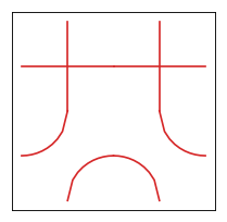
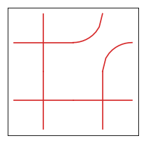
Refer to caption
Refer to caption
Refer to caption
Figure 9: First figure: two contractible loops. Indeed, you cannot follow any of the two loops from top to bottom without crossing the vertical periodic boundary. Second figure: two odd non-contractible loops, and one contractible loop. Indeed, the horizontal line at the bottom is a contractible loop, and the two other loops are non-contractible and cross the vertical periodic boundary exactly once. Third figure: one even non-contractible loop. Indeed, there is only one loop that crosses the vertical periodic boundary twice. If we now denote with a diagram like ∙\bullet∙\bullet∙\bullet∙\bullet the connections between the four beginnings of strands ∙\bullet at the top and the bottom of the lattice, then the strands in the first figure are connected like ∙\bullet∙\bullet∙\bullet∙\bullet, in the second figure like ∙\bullet∙\bullet∙\bullet∙\bullet, and in the last figure like ∙\bullet∙\bullet∙\bullet∙\bullet.

6.2 Inclusion of o​s​posp spectra

To prove the inclusion of the spectra for the o​s​posp chains, another lemma is needed:

Lemma 2.

If AA and MM are square matrices of size nn and n+mn+m such that

∀k∈ℕ,∀i,j∈{1,…,n},(Mk)i,j=(Ak)i,j,\forall k\in\mathbb{N}\,,\quad\forall i,j\in\{1,...,n\}\,,\quad(M^{k})_{i,j}=(A^{k})_{i,j}\,, (178)

then the spectrum of AA is included in the spectrum of MM (with the degeneracies).

Proof.

Writing MM in block form

M=(ABCD),M=\left(\begin{matrix}A&B\\ C&D\end{matrix}\right)\,, (179)

the condition (178) implies

∀k∈ℕ,B​Dk​C=0.\forall k\in\mathbb{N},\quad BD^{k}C=0\,. (180)

Let now λ∈ℂ\lambda\in\mathbb{C} not in the spectrum of DD. Since D−λ​ImD-\lambda I_{m} is invertible one can use Schur’s complement to write

det(M−λ​In+m)=det(A−λ​In−B​(D−λ​Im)−1​C)​det(D−λ​Im).\det(M-\lambda I_{n+m})=\det(A-\lambda I_{n}-B(D-\lambda I_{m})^{-1}C)\det(D-\lambda I_{m})\,. (181)

From Cayley-Hamilton theorem, (D−λ​Im)−1(D-\lambda I_{m})^{-1} is a polynomial in (D−λ​Im)(D-\lambda I_{m}), thus in DD, so that with (180) we have B​(D−λ​Im)−1​C=0B(D-\lambda I_{m})^{-1}C=0. It follows that

det(M−λ​In+m)=det(A−λ​In)​det(D−λ​Im).\det(M-\lambda I_{n+m})=\det(A-\lambda I_{n})\det(D-\lambda I_{m})\,. (182)

Since the function λ→det(M−λ​In+m)\lambda\to\det(M-\lambda I_{n+m}) is continuous in λ\lambda and since the spectrum of DD is finite, the previous equation is true for all λ∈ℂ\lambda\in\mathbb{C}. Thus whenever λ\lambda is an eigenvalue of AA, det(M−λ​In+m)=0\det(M-\lambda I_{n+m})=0 and it is also an eigenvalue of MM. Moreover since det(D−λ​Im)\det(D-\lambda I_{m}) is a polynomial in λ\lambda there cannot be poles and the eigenvalues of AA in the spectrum of MM have at least the degeneracies they have in the spectrum of AA. (However in general the eigenvectors of MM corresponding to the eigenvalues of AA cannot be expressed simply: in particular they may have non-zero ii-th components for i>ni>n.) ∎

One can now prove the theorem:

Theorem 2 (Inclusion of spectra).

The spectrum of the o​s​p​(r|2​s)osp(r|2s) spin chain is included in finite size in the spectrum of the o​s​p​(r+p|2​s+p)osp(r+p|2s+p) spin chain for all even p>0p>0.

Proof.

Denote tt the transfer matrix of the o​s​p​(r|2​s)osp(r|2s) spin chain, and TT the one of the o​s​p​(r+p|2​s+p)osp(r+p|2s+p) spin chain. Let JJ be a subset of 2​p2p indices among which pp are bosonic and pp are fermionic, and I={1,…,r+2​s+2​p}∖JI=\{1,...,r+2s+2p\}\setminus J. The indices of tt are identified with II.

(TM)α11​…​αL1α1M+1​…​αLM+1(T^{M})^{\alpha_{1}^{M+1}...\alpha_{L}^{M+1}}_{\alpha_{1}^{1}...\alpha_{L}^{1}} is the partition function of the model on a L×ML\times M lattice with fixed boundary conditions at the top and bottom boundaries. Inside the configuration, every loop whose index is in JJ has to be contractible, since at the up and down boundaries the indices must be in II. As JJ contains as many bosonic as fermionic indices, lemma 1 implies that these configurations add up to zero. Therefore all the loops can be considered having their indices in II, which is exactly (tM)α11​…​αL1α1M+1​…​αLM+1(t^{M})^{\alpha_{1}^{M+1}...\alpha_{L}^{M+1}}_{\alpha_{1}^{1}...\alpha_{L}^{1}}. Then lemma 2 applies and proves the theorem. ∎

Note that taking the supertrace of the monodromy matrix is crucial to have this property. Otherwise the non-contractible loops in the horizontal direction would not cancel out. Notice also that integrability does not play any role here, so it is true for arbitrary weights in the RR-matrix. Recall that such an inclusion is observed for g​l​(r|s)gl(r|s) models as well [50].

6.3 Charges and loop configurations

While most of our discussion about critical exponents has been based on studies of the integrable Hamiltonian, it is usually the case that the same universal properties would be obtained by focussing instead on the transfer matrix. Indeed, taking the Hamiltonian limit amounts to taking the continuum limit in the (imaginary) time direction, something that is not supposed to modify the continuum description of the lattice model. The transfer matrix language is on the other hand more natural to describe loops, especially when the spectral parameter λ=1\lambda=1, corresponding to an isotropic loop soup on the square lattice. We have checked that the log of the largest eigenvalues of the transfer matrix have the same behaviour as those of the Hamiltonian (21), simply with the Fermi velocity vFv_{F} replaced by a sound velocity sin⁡(λ​vF)\sin(\lambda v_{F}), that is 11 at the isotropic point.

This means that the finite-size corrections to the first excited states of the Hamiltonian, among which are the lowest eigenvalues in a sector imposing specific values of charges, correspond in the transfer matrix point of view to finite-size corrections to the largest eigenvalues of the transfer matrix tt in a sub vector space with specific values of charges. We recall that the partition function in (176) is given by the trace of the MM-th power of t=t⁡(λ)t=t(\lambda) the transfer matrix, that is dominated when M→∞M\to\infty by the largest eigenvalue of tt. Similarly, the trace of the MM-th power of tt over a sub vector space where the charges take specific values, is dominated by the largest eigenvalue of tt in this sub vector space.

The question is now to understand the kind of constraint that is imposed on the intersecting loop soup when this trace over a sub vector space where the charges take specific values is performed.

Let us treat the case of o​s​p​(2|2)osp(2|2), the simplest example with a “fermionic charge” JzJ_{z} and a “bosonic charge” QzQ_{z}. In the grading given by (11), they are represented by

2​Jz=(100000000000000−1),2​Qz=(0000010000−100000).2J_{z}=\left(\begin{matrix}1&0&0&0\\ 0&0&0&0\\ 0&0&0&0\\ 0&0&0&-1\end{matrix}\right)\,,\quad 2Q_{z}=\left(\begin{matrix}0&0&0&0\\ 0&1&0&0\\ 0&0&-1&0\\ 0&0&0&0\end{matrix}\right)\,. (183)

When one traces over the vector space where QzQ_{z} is equal to qq, one considers only the configurations where at the bottom (and at the top) of the lattice, there are 2​q2q more strands with index 22 than strands with index 33. As already said, along a loop an index ii is replaced by its conjugate i′i^{\prime} (i.e., 1↔41\leftrightarrow 4, 2↔32\leftrightarrow 3 ) every time a NW or SE corner is encountered. It implies that a strand carrying a 22 at the bottom cannot directly (without crossing the vertical boundary) join another strand carrying a 22 at the bottom. Then the 2​q2q extra 22’s at the bottom and at the top of the lattice have to be connected between themselves by going through the whole lattice in the vertical direction. Since the loops with bosonic index (whether contractible or not) are always given the same weight equal to 11, it comes, after summing over the indices, that the boundary condition imposes to have (at least) 2​q2q loops that propagate through the lattice in the vertical direction that are given weight 11. Note that an extra strand with index 22 at the bottom can be connected to any extra strand with index 22 at the top, with the same weight 11. For 2​q=22q=2 these configurations are            ∙   ∙   ∙   ∙     +           ∙   ∙   ∙   ∙     \hbox to14.61pt{\vbox to17.67pt{\pgfpicture\makeatletter\hbox{\hskip 5.1733pt\lower-8.83359pt\hbox to0.0pt{\lxSVG@begingroup@{_scopebegin=1} \lxSVG@begingroup@{stroke=#000000} \lxSVG@begingroup@{fill=#000000} \lxSVG@setlinewidth{\the\pgflinewidth}\lxSVG@begingroup@{stroke-width=0.4pt} \lx@inpgf@ignorespaces\nullfont\hbox to0.0pt{\lxSVG@begingroup@{_scopebegin=1} {{\lx@inpgf@ignorespaces}} {}{{}}{} {}{}\lxSVG@begingroup@{_scopebegin=1} \color[rgb]{0,0,0}\lxSVG@setlinewidth{\the\pgflinewidth}\lxSVG@begingroup@{stroke-width=1.0pt} \lx@inpgf@ignorespaces{}\lxSVG@stroke\lxSVG@drawpath@unclipped{M 0 -5.91 L 0 5.91}{fill:none} \lx@inpgf@ignorespaces \lxSVG@closescope {}{{}}{} {}{}\lxSVG@begingroup@{_scopebegin=1} \color[rgb]{0,0,0}\lxSVG@setlinewidth{\the\pgflinewidth}\lxSVG@begingroup@{stroke-width=1.0pt} \lx@inpgf@ignorespaces{}\lxSVG@stroke\lxSVG@drawpath@unclipped{M 5.91 -5.91 L 5.91 5.91}{fill:none} \lx@inpgf@ignorespaces \lxSVG@closescope {{}}\lx@inpgf@ignorespaces\hbox{\hbox{{\lxSVG@begingroup@{_scopebegin=1} {{}{}{{ {}{}}}{ {}{}} {{}{{\lx@inpgf@ignorespaces}}}{{}{\lx@inpgf@ignorespaces}}{}{{}{\lx@inpgf@ignorespaces}} {\lx@inpgf@ignorespaces }{{{{\lx@inpgf@ignorespaces}}\lxSVG@begingroup@{_scopebegin=1} \lxSVG@transformcm{1.0}{0.0}{0.0}{1.0}{-1.84029pt}{-5.50058pt}\lxSVG@begingroup@{transform=matrix(1.0 0.0 0.0 1.0 -2.55 -7.61)} \pgfsys@hbox{58}\lxSVG@closescope }}} \lxSVG@closescope }}} {{}}\lx@inpgf@ignorespaces\hbox{\hbox{{\lxSVG@begingroup@{_scopebegin=1} {{}{}{{ {}{}}}{ {}{}} {{}{{\lx@inpgf@ignorespaces}}}{{}{\lx@inpgf@ignorespaces}}{}{{}{\lx@inpgf@ignorespaces}} {\lx@inpgf@ignorespaces }{{{{\lx@inpgf@ignorespaces}}\lxSVG@begingroup@{_scopebegin=1} \lxSVG@transformcm{1.0}{0.0}{0.0}{1.0}{-1.84029pt}{3.03531pt}\lxSVG@begingroup@{transform=matrix(1.0 0.0 0.0 1.0 -2.55 4.2)} \pgfsys@hbox{58}\lxSVG@closescope }}} \lxSVG@closescope }}} {{}}\lx@inpgf@ignorespaces\hbox{\hbox{{\lxSVG@begingroup@{_scopebegin=1} {{}{}{{ {}{}}}{ {}{}} {{}{{\lx@inpgf@ignorespaces}}}{{}{\lx@inpgf@ignorespaces}}{}{{}{\lx@inpgf@ignorespaces}} {\lx@inpgf@ignorespaces }{{{{\lx@inpgf@ignorespaces}}\lxSVG@begingroup@{_scopebegin=1} \lxSVG@transformcm{1.0}{0.0}{0.0}{1.0}{2.42766pt}{-5.50058pt}\lxSVG@begingroup@{transform=matrix(1.0 0.0 0.0 1.0 3.36 -7.61)} \pgfsys@hbox{58}\lxSVG@closescope }}} \lxSVG@closescope }}} {{}}\lx@inpgf@ignorespaces\hbox{\hbox{{\lxSVG@begingroup@{_scopebegin=1} {{}{}{{ {}{}}}{ {}{}} {{}{{\lx@inpgf@ignorespaces}}}{{}{\lx@inpgf@ignorespaces}}{}{{}{\lx@inpgf@ignorespaces}} {\lx@inpgf@ignorespaces }{{{{\lx@inpgf@ignorespaces}}\lxSVG@begingroup@{_scopebegin=1} \lxSVG@transformcm{1.0}{0.0}{0.0}{1.0}{2.42766pt}{3.03531pt}\lxSVG@begingroup@{transform=matrix(1.0 0.0 0.0 1.0 3.36 4.2)} \pgfsys@hbox{58}\lxSVG@closescope }}} \lxSVG@closescope }}} \lxSVG@closescope {\lx@inpgf@ignorespaces}{\lx@inpgf@ignorespaces}{\lx@inpgf@ignorespaces}\hss}\lxSVG@discardpath\lxSVG@closescope \hss}}\lxSVG@closescope\endpgfpicture}}+\hbox to14.61pt{\vbox to17.67pt{\pgfpicture\makeatletter\hbox{\hskip 5.1733pt\lower-8.83359pt\hbox to0.0pt{\lxSVG@begingroup@{_scopebegin=1} \lxSVG@begingroup@{stroke=#000000} \lxSVG@begingroup@{fill=#000000} \lxSVG@setlinewidth{\the\pgflinewidth}\lxSVG@begingroup@{stroke-width=0.4pt} \lx@inpgf@ignorespaces\nullfont\hbox to0.0pt{\lxSVG@begingroup@{_scopebegin=1} {{\lx@inpgf@ignorespaces}} {}{{}}{} {}{}\lxSVG@begingroup@{_scopebegin=1} \color[rgb]{0,0,0}\lxSVG@setlinewidth{\the\pgflinewidth}\lxSVG@begingroup@{stroke-width=1.0pt} \lx@inpgf@ignorespaces{}\lxSVG@stroke\lxSVG@drawpath@unclipped{M 0 -5.91 L 5.91 5.91}{fill:none} \lx@inpgf@ignorespaces \lxSVG@closescope {}{{}}{} {}{}\lxSVG@begingroup@{_scopebegin=1} \color[rgb]{0,0,0}\lxSVG@setlinewidth{\the\pgflinewidth}\lxSVG@begingroup@{stroke-width=1.0pt} \lx@inpgf@ignorespaces{}\lxSVG@stroke\lxSVG@drawpath@unclipped{M 5.91 -5.91 L 0 5.91}{fill:none} \lx@inpgf@ignorespaces \lxSVG@closescope {{}}\lx@inpgf@ignorespaces\hbox{\hbox{{\lxSVG@begingroup@{_scopebegin=1} {{}{}{{ {}{}}}{ {}{}} {{}{{\lx@inpgf@ignorespaces}}}{{}{\lx@inpgf@ignorespaces}}{}{{}{\lx@inpgf@ignorespaces}} {\lx@inpgf@ignorespaces }{{{{\lx@inpgf@ignorespaces}}\lxSVG@begingroup@{_scopebegin=1} \lxSVG@transformcm{1.0}{0.0}{0.0}{1.0}{-1.84029pt}{-5.50058pt}\lxSVG@begingroup@{transform=matrix(1.0 0.0 0.0 1.0 -2.55 -7.61)} \pgfsys@hbox{58}\lxSVG@closescope }}} \lxSVG@closescope }}} {{}}\lx@inpgf@ignorespaces\hbox{\hbox{{\lxSVG@begingroup@{_scopebegin=1} {{}{}{{ {}{}}}{ {}{}} {{}{{\lx@inpgf@ignorespaces}}}{{}{\lx@inpgf@ignorespaces}}{}{{}{\lx@inpgf@ignorespaces}} {\lx@inpgf@ignorespaces }{{{{\lx@inpgf@ignorespaces}}\lxSVG@begingroup@{_scopebegin=1} \lxSVG@transformcm{1.0}{0.0}{0.0}{1.0}{-1.84029pt}{3.03531pt}\lxSVG@begingroup@{transform=matrix(1.0 0.0 0.0 1.0 -2.55 4.2)} \pgfsys@hbox{58}\lxSVG@closescope }}} \lxSVG@closescope }}} {{}}\lx@inpgf@ignorespaces\hbox{\hbox{{\lxSVG@begingroup@{_scopebegin=1} {{}{}{{ {}{}}}{ {}{}} {{}{{\lx@inpgf@ignorespaces}}}{{}{\lx@inpgf@ignorespaces}}{}{{}{\lx@inpgf@ignorespaces}} {\lx@inpgf@ignorespaces }{{{{\lx@inpgf@ignorespaces}}\lxSVG@begingroup@{_scopebegin=1} \lxSVG@transformcm{1.0}{0.0}{0.0}{1.0}{2.42766pt}{-5.50058pt}\lxSVG@begingroup@{transform=matrix(1.0 0.0 0.0 1.0 3.36 -7.61)} \pgfsys@hbox{58}\lxSVG@closescope }}} \lxSVG@closescope }}} {{}}\lx@inpgf@ignorespaces\hbox{\hbox{{\lxSVG@begingroup@{_scopebegin=1} {{}{}{{ {}{}}}{ {}{}} {{}{{\lx@inpgf@ignorespaces}}}{{}{\lx@inpgf@ignorespaces}}{}{{}{\lx@inpgf@ignorespaces}} {\lx@inpgf@ignorespaces }{{{{\lx@inpgf@ignorespaces}}\lxSVG@begingroup@{_scopebegin=1} \lxSVG@transformcm{1.0}{0.0}{0.0}{1.0}{2.42766pt}{3.03531pt}\lxSVG@begingroup@{transform=matrix(1.0 0.0 0.0 1.0 3.36 4.2)} \pgfsys@hbox{58}\lxSVG@closescope }}} \lxSVG@closescope }}} \lxSVG@closescope {\lx@inpgf@ignorespaces}{\lx@inpgf@ignorespaces}{\lx@inpgf@ignorespaces}\hss}\lxSVG@discardpath\lxSVG@closescope \hss}}\lxSVG@closescope\endpgfpicture}}.

If one traces over the vector space where JzJ_{z} is equal to jj, the same reasoning shows that the configurations are constrained to have 2​j2j more strands with index 11 than index 44 at the bottom, and that those at the top and the bottom of the lattice have to be connected between themselves. However since the index is fermionic, the weight of such a loop is 11 (resp. −1-1) if it crosses the top and bottom boundary an odd (resp. even) number of times, from lemma 1. The total weight given to these loops is then exactly the signature of the permutation that maps the bottom 2​j2j extra 11’s to the top 2​j2j extra 11’s they are connected to. For 2​j=22j=2 these configurations are            ∙   ∙   ∙   ∙     −           ∙   ∙   ∙   ∙     \hbox to14.61pt{\vbox to17.67pt{\pgfpicture\makeatletter\hbox{\hskip 5.1733pt\lower-8.83359pt\hbox to0.0pt{\lxSVG@begingroup@{_scopebegin=1} \lxSVG@begingroup@{stroke=#000000} \lxSVG@begingroup@{fill=#000000} \lxSVG@setlinewidth{\the\pgflinewidth}\lxSVG@begingroup@{stroke-width=0.4pt} \lx@inpgf@ignorespaces\nullfont\hbox to0.0pt{\lxSVG@begingroup@{_scopebegin=1} {{\lx@inpgf@ignorespaces}} {}{{}}{} {}{}\lxSVG@begingroup@{_scopebegin=1} \color[rgb]{0,0,0}\lxSVG@setlinewidth{\the\pgflinewidth}\lxSVG@begingroup@{stroke-width=1.0pt} \lx@inpgf@ignorespaces{}\lxSVG@stroke\lxSVG@drawpath@unclipped{M 0 -5.91 L 0 5.91}{fill:none} \lx@inpgf@ignorespaces \lxSVG@closescope {}{{}}{} {}{}\lxSVG@begingroup@{_scopebegin=1} \color[rgb]{0,0,0}\lxSVG@setlinewidth{\the\pgflinewidth}\lxSVG@begingroup@{stroke-width=1.0pt} \lx@inpgf@ignorespaces{}\lxSVG@stroke\lxSVG@drawpath@unclipped{M 5.91 -5.91 L 5.91 5.91}{fill:none} \lx@inpgf@ignorespaces \lxSVG@closescope {{}}\lx@inpgf@ignorespaces\hbox{\hbox{{\lxSVG@begingroup@{_scopebegin=1} {{}{}{{ {}{}}}{ {}{}} {{}{{\lx@inpgf@ignorespaces}}}{{}{\lx@inpgf@ignorespaces}}{}{{}{\lx@inpgf@ignorespaces}} {\lx@inpgf@ignorespaces }{{{{\lx@inpgf@ignorespaces}}\lxSVG@begingroup@{_scopebegin=1} \lxSVG@transformcm{1.0}{0.0}{0.0}{1.0}{-1.84029pt}{-5.50058pt}\lxSVG@begingroup@{transform=matrix(1.0 0.0 0.0 1.0 -2.55 -7.61)} \pgfsys@hbox{58}\lxSVG@closescope }}} \lxSVG@closescope }}} {{}}\lx@inpgf@ignorespaces\hbox{\hbox{{\lxSVG@begingroup@{_scopebegin=1} {{}{}{{ {}{}}}{ {}{}} {{}{{\lx@inpgf@ignorespaces}}}{{}{\lx@inpgf@ignorespaces}}{}{{}{\lx@inpgf@ignorespaces}} {\lx@inpgf@ignorespaces }{{{{\lx@inpgf@ignorespaces}}\lxSVG@begingroup@{_scopebegin=1} \lxSVG@transformcm{1.0}{0.0}{0.0}{1.0}{-1.84029pt}{3.03531pt}\lxSVG@begingroup@{transform=matrix(1.0 0.0 0.0 1.0 -2.55 4.2)} \pgfsys@hbox{58}\lxSVG@closescope }}} \lxSVG@closescope }}} {{}}\lx@inpgf@ignorespaces\hbox{\hbox{{\lxSVG@begingroup@{_scopebegin=1} {{}{}{{ {}{}}}{ {}{}} {{}{{\lx@inpgf@ignorespaces}}}{{}{\lx@inpgf@ignorespaces}}{}{{}{\lx@inpgf@ignorespaces}} {\lx@inpgf@ignorespaces }{{{{\lx@inpgf@ignorespaces}}\lxSVG@begingroup@{_scopebegin=1} \lxSVG@transformcm{1.0}{0.0}{0.0}{1.0}{2.42766pt}{-5.50058pt}\lxSVG@begingroup@{transform=matrix(1.0 0.0 0.0 1.0 3.36 -7.61)} \pgfsys@hbox{58}\lxSVG@closescope }}} \lxSVG@closescope }}} {{}}\lx@inpgf@ignorespaces\hbox{\hbox{{\lxSVG@begingroup@{_scopebegin=1} {{}{}{{ {}{}}}{ {}{}} {{}{{\lx@inpgf@ignorespaces}}}{{}{\lx@inpgf@ignorespaces}}{}{{}{\lx@inpgf@ignorespaces}} {\lx@inpgf@ignorespaces }{{{{\lx@inpgf@ignorespaces}}\lxSVG@begingroup@{_scopebegin=1} \lxSVG@transformcm{1.0}{0.0}{0.0}{1.0}{2.42766pt}{3.03531pt}\lxSVG@begingroup@{transform=matrix(1.0 0.0 0.0 1.0 3.36 4.2)} \pgfsys@hbox{58}\lxSVG@closescope }}} \lxSVG@closescope }}} \lxSVG@closescope {\lx@inpgf@ignorespaces}{\lx@inpgf@ignorespaces}{\lx@inpgf@ignorespaces}\hss}\lxSVG@discardpath\lxSVG@closescope \hss}}\lxSVG@closescope\endpgfpicture}}-\hbox to14.61pt{\vbox to17.67pt{\pgfpicture\makeatletter\hbox{\hskip 5.1733pt\lower-8.83359pt\hbox to0.0pt{\lxSVG@begingroup@{_scopebegin=1} \lxSVG@begingroup@{stroke=#000000} \lxSVG@begingroup@{fill=#000000} \lxSVG@setlinewidth{\the\pgflinewidth}\lxSVG@begingroup@{stroke-width=0.4pt} \lx@inpgf@ignorespaces\nullfont\hbox to0.0pt{\lxSVG@begingroup@{_scopebegin=1} {{\lx@inpgf@ignorespaces}} {}{{}}{} {}{}\lxSVG@begingroup@{_scopebegin=1} \color[rgb]{0,0,0}\lxSVG@setlinewidth{\the\pgflinewidth}\lxSVG@begingroup@{stroke-width=1.0pt} \lx@inpgf@ignorespaces{}\lxSVG@stroke\lxSVG@drawpath@unclipped{M 0 -5.91 L 5.91 5.91}{fill:none} \lx@inpgf@ignorespaces \lxSVG@closescope {}{{}}{} {}{}\lxSVG@begingroup@{_scopebegin=1} \color[rgb]{0,0,0}\lxSVG@setlinewidth{\the\pgflinewidth}\lxSVG@begingroup@{stroke-width=1.0pt} \lx@inpgf@ignorespaces{}\lxSVG@stroke\lxSVG@drawpath@unclipped{M 5.91 -5.91 L 0 5.91}{fill:none} \lx@inpgf@ignorespaces \lxSVG@closescope {{}}\lx@inpgf@ignorespaces\hbox{\hbox{{\lxSVG@begingroup@{_scopebegin=1} {{}{}{{ {}{}}}{ {}{}} {{}{{\lx@inpgf@ignorespaces}}}{{}{\lx@inpgf@ignorespaces}}{}{{}{\lx@inpgf@ignorespaces}} {\lx@inpgf@ignorespaces }{{{{\lx@inpgf@ignorespaces}}\lxSVG@begingroup@{_scopebegin=1} \lxSVG@transformcm{1.0}{0.0}{0.0}{1.0}{-1.84029pt}{-5.50058pt}\lxSVG@begingroup@{transform=matrix(1.0 0.0 0.0 1.0 -2.55 -7.61)} \pgfsys@hbox{58}\lxSVG@closescope }}} \lxSVG@closescope }}} {{}}\lx@inpgf@ignorespaces\hbox{\hbox{{\lxSVG@begingroup@{_scopebegin=1} {{}{}{{ {}{}}}{ {}{}} {{}{{\lx@inpgf@ignorespaces}}}{{}{\lx@inpgf@ignorespaces}}{}{{}{\lx@inpgf@ignorespaces}} {\lx@inpgf@ignorespaces }{{{{\lx@inpgf@ignorespaces}}\lxSVG@begingroup@{_scopebegin=1} \lxSVG@transformcm{1.0}{0.0}{0.0}{1.0}{-1.84029pt}{3.03531pt}\lxSVG@begingroup@{transform=matrix(1.0 0.0 0.0 1.0 -2.55 4.2)} \pgfsys@hbox{58}\lxSVG@closescope }}} \lxSVG@closescope }}} {{}}\lx@inpgf@ignorespaces\hbox{\hbox{{\lxSVG@begingroup@{_scopebegin=1} {{}{}{{ {}{}}}{ {}{}} {{}{{\lx@inpgf@ignorespaces}}}{{}{\lx@inpgf@ignorespaces}}{}{{}{\lx@inpgf@ignorespaces}} {\lx@inpgf@ignorespaces }{{{{\lx@inpgf@ignorespaces}}\lxSVG@begingroup@{_scopebegin=1} \lxSVG@transformcm{1.0}{0.0}{0.0}{1.0}{2.42766pt}{-5.50058pt}\lxSVG@begingroup@{transform=matrix(1.0 0.0 0.0 1.0 3.36 -7.61)} \pgfsys@hbox{58}\lxSVG@closescope }}} \lxSVG@closescope }}} {{}}\lx@inpgf@ignorespaces\hbox{\hbox{{\lxSVG@begingroup@{_scopebegin=1} {{}{}{{ {}{}}}{ {}{}} {{}{{\lx@inpgf@ignorespaces}}}{{}{\lx@inpgf@ignorespaces}}{}{{}{\lx@inpgf@ignorespaces}} {\lx@inpgf@ignorespaces }{{{{\lx@inpgf@ignorespaces}}\lxSVG@begingroup@{_scopebegin=1} \lxSVG@transformcm{1.0}{0.0}{0.0}{1.0}{2.42766pt}{3.03531pt}\lxSVG@begingroup@{transform=matrix(1.0 0.0 0.0 1.0 3.36 4.2)} \pgfsys@hbox{58}\lxSVG@closescope }}} \lxSVG@closescope }}} \lxSVG@closescope {\lx@inpgf@ignorespaces}{\lx@inpgf@ignorespaces}{\lx@inpgf@ignorespaces}\hss}\lxSVG@discardpath\lxSVG@closescope \hss}}\lxSVG@closescope\endpgfpicture}}.

If one traces over the vector space where both JzJ_{z} and QzQ_{z} are fixed as jj and qq respectively, then the configurations are constrained to possess 2​j2j strands with index 11 and 2​q2q strands with index 22 to propagate through the lattice from bottom to top. The total weight given to these loops is then the signature ϵ⁡(σj)\epsilon(\sigma_{j}) of the permutation σj\sigma_{j} that maps the bottom 2​j2j extra 11’s to the top 2​j2j extra 11’s they are connected to, without considering the 2​q2q bosonic strands. Let us now denote PL,M​(σ)P_{L,M}(\sigma) the sum of all the configurations on a L×ML\times M lattice with 2​j+2​q2j+2q non-contractible strands, where the 2​j2j ’fermionic’ strands are at the left of the lattice at row 11, and where the 2​j+2​q2j+2q strands are permuted by σ\sigma at row MM. Since a fermionic strand has to be connected to another fermionic strand through the periodic vertical boundary, this permutation has to be decomposable into σ=σj​σq\sigma=\sigma_{j}\sigma_{q} where σj\sigma_{j} acts trivially on the bosonic strands and σq\sigma_{q} trivially on the fermionic strands. Then, denoting by trj,q\,\text{tr}\,_{j,q} the trace over the sector Jz=j,Qz=qJ_{z}=j,Q_{z}=q, one can express the trace of the MM-th power of the transfer matrix tt as

trj,q​(tM)=∑σj,σqϵ⁡(σj)​ZL,M​(σj​σq),\,\text{tr}\,_{j,q}(t^{M})=\sum_{\sigma_{j},\sigma_{q}}\epsilon(\sigma_{j})Z_{L,M}(\sigma_{j}\sigma_{q})\,, (184)

where the sum runs over the permutations σj\sigma_{j} and σq\sigma_{q} of 2​j+2​q2j+2q elements, that leave invariant the last 2​q2q elements (respectively the first 2​j2j elements). We recall that ϵ⁡(σj)\epsilon(\sigma_{j}) is the signature of the permutation σj\sigma_{j}. Here are some examples:

tr1,0​(tM)\displaystyle\,\text{tr}\,_{1,0}(t^{M}) =ZL​M​((1 2))−ZL​M​((2 1))\displaystyle=Z_{LM}((1\,2))-Z_{LM}((2\,1)) (185)
tr0,1​(tM)\displaystyle\,\text{tr}\,_{0,1}(t^{M}) =ZL​M​((1 2))+ZL​M​((2 1))\displaystyle=Z_{LM}((1\,2))+Z_{LM}((2\,1))
tr1,1​(tM)\displaystyle\,\text{tr}\,_{1,1}(t^{M}) =ZL​M​((1 2 3 4))−ZL​M​((2 1 3 4))+ZL​M​((1 2 4 3))−ZL​M​((2 1 4 3))\displaystyle=Z_{LM}((1\,2\,3\,4))-Z_{LM}((2\,1\,3\,4))+Z_{LM}((1\,2\,4\,3))-Z_{LM}((2\,1\,4\,3))

where we write (i1​…​in)(i_{1}\,...\,i_{n}) the permutation that maps 11 onto i1i_{1}, etc, nn onto ini_{n}. The configuration of strands connections to which these three traces correspond are respectively            ∙   ∙   ∙   ∙     −           ∙   ∙   ∙   ∙     \hbox to14.61pt{\vbox to17.67pt{\pgfpicture\makeatletter\hbox{\hskip 5.1733pt\lower-8.83359pt\hbox to0.0pt{\lxSVG@begingroup@{_scopebegin=1} \lxSVG@begingroup@{stroke=#000000} \lxSVG@begingroup@{fill=#000000} \lxSVG@setlinewidth{\the\pgflinewidth}\lxSVG@begingroup@{stroke-width=0.4pt} \lx@inpgf@ignorespaces\nullfont\hbox to0.0pt{\lxSVG@begingroup@{_scopebegin=1} {{\lx@inpgf@ignorespaces}} {}{{}}{} {}{}\lxSVG@begingroup@{_scopebegin=1} \color[rgb]{0,0,0}\lxSVG@setlinewidth{\the\pgflinewidth}\lxSVG@begingroup@{stroke-width=1.0pt} \lx@inpgf@ignorespaces{}\lxSVG@stroke\lxSVG@drawpath@unclipped{M 0 -5.91 L 0 5.91}{fill:none} \lx@inpgf@ignorespaces \lxSVG@closescope {}{{}}{} {}{}\lxSVG@begingroup@{_scopebegin=1} \color[rgb]{0,0,0}\lxSVG@setlinewidth{\the\pgflinewidth}\lxSVG@begingroup@{stroke-width=1.0pt} \lx@inpgf@ignorespaces{}\lxSVG@stroke\lxSVG@drawpath@unclipped{M 5.91 -5.91 L 5.91 5.91}{fill:none} \lx@inpgf@ignorespaces \lxSVG@closescope {{}}\lx@inpgf@ignorespaces\hbox{\hbox{{\lxSVG@begingroup@{_scopebegin=1} {{}{}{{ {}{}}}{ {}{}} {{}{{\lx@inpgf@ignorespaces}}}{{}{\lx@inpgf@ignorespaces}}{}{{}{\lx@inpgf@ignorespaces}} {\lx@inpgf@ignorespaces }{{{{\lx@inpgf@ignorespaces}}\lxSVG@begingroup@{_scopebegin=1} \lxSVG@transformcm{1.0}{0.0}{0.0}{1.0}{-1.84029pt}{-5.50058pt}\lxSVG@begingroup@{transform=matrix(1.0 0.0 0.0 1.0 -2.55 -7.61)} \pgfsys@hbox{58}\lxSVG@closescope }}} \lxSVG@closescope }}} {{}}\lx@inpgf@ignorespaces\hbox{\hbox{{\lxSVG@begingroup@{_scopebegin=1} {{}{}{{ {}{}}}{ {}{}} {{}{{\lx@inpgf@ignorespaces}}}{{}{\lx@inpgf@ignorespaces}}{}{{}{\lx@inpgf@ignorespaces}} {\lx@inpgf@ignorespaces }{{{{\lx@inpgf@ignorespaces}}\lxSVG@begingroup@{_scopebegin=1} \lxSVG@transformcm{1.0}{0.0}{0.0}{1.0}{-1.84029pt}{3.03531pt}\lxSVG@begingroup@{transform=matrix(1.0 0.0 0.0 1.0 -2.55 4.2)} \pgfsys@hbox{58}\lxSVG@closescope }}} \lxSVG@closescope }}} {{}}\lx@inpgf@ignorespaces\hbox{\hbox{{\lxSVG@begingroup@{_scopebegin=1} {{}{}{{ {}{}}}{ {}{}} {{}{{\lx@inpgf@ignorespaces}}}{{}{\lx@inpgf@ignorespaces}}{}{{}{\lx@inpgf@ignorespaces}} {\lx@inpgf@ignorespaces }{{{{\lx@inpgf@ignorespaces}}\lxSVG@begingroup@{_scopebegin=1} \lxSVG@transformcm{1.0}{0.0}{0.0}{1.0}{2.42766pt}{-5.50058pt}\lxSVG@begingroup@{transform=matrix(1.0 0.0 0.0 1.0 3.36 -7.61)} \pgfsys@hbox{58}\lxSVG@closescope }}} \lxSVG@closescope }}} {{}}\lx@inpgf@ignorespaces\hbox{\hbox{{\lxSVG@begingroup@{_scopebegin=1} {{}{}{{ {}{}}}{ {}{}} {{}{{\lx@inpgf@ignorespaces}}}{{}{\lx@inpgf@ignorespaces}}{}{{}{\lx@inpgf@ignorespaces}} {\lx@inpgf@ignorespaces }{{{{\lx@inpgf@ignorespaces}}\lxSVG@begingroup@{_scopebegin=1} \lxSVG@transformcm{1.0}{0.0}{0.0}{1.0}{2.42766pt}{3.03531pt}\lxSVG@begingroup@{transform=matrix(1.0 0.0 0.0 1.0 3.36 4.2)} \pgfsys@hbox{58}\lxSVG@closescope }}} \lxSVG@closescope }}} \lxSVG@closescope {\lx@inpgf@ignorespaces}{\lx@inpgf@ignorespaces}{\lx@inpgf@ignorespaces}\hss}\lxSVG@discardpath\lxSVG@closescope \hss}}\lxSVG@closescope\endpgfpicture}}-\hbox to14.61pt{\vbox to17.67pt{\pgfpicture\makeatletter\hbox{\hskip 5.1733pt\lower-8.83359pt\hbox to0.0pt{\lxSVG@begingroup@{_scopebegin=1} \lxSVG@begingroup@{stroke=#000000} \lxSVG@begingroup@{fill=#000000} \lxSVG@setlinewidth{\the\pgflinewidth}\lxSVG@begingroup@{stroke-width=0.4pt} \lx@inpgf@ignorespaces\nullfont\hbox to0.0pt{\lxSVG@begingroup@{_scopebegin=1} {{\lx@inpgf@ignorespaces}} {}{{}}{} {}{}\lxSVG@begingroup@{_scopebegin=1} \color[rgb]{0,0,0}\lxSVG@setlinewidth{\the\pgflinewidth}\lxSVG@begingroup@{stroke-width=1.0pt} \lx@inpgf@ignorespaces{}\lxSVG@stroke\lxSVG@drawpath@unclipped{M 0 -5.91 L 5.91 5.91}{fill:none} \lx@inpgf@ignorespaces \lxSVG@closescope {}{{}}{} {}{}\lxSVG@begingroup@{_scopebegin=1} \color[rgb]{0,0,0}\lxSVG@setlinewidth{\the\pgflinewidth}\lxSVG@begingroup@{stroke-width=1.0pt} \lx@inpgf@ignorespaces{}\lxSVG@stroke\lxSVG@drawpath@unclipped{M 5.91 -5.91 L 0 5.91}{fill:none} \lx@inpgf@ignorespaces \lxSVG@closescope {{}}\lx@inpgf@ignorespaces\hbox{\hbox{{\lxSVG@begingroup@{_scopebegin=1} {{}{}{{ {}{}}}{ {}{}} {{}{{\lx@inpgf@ignorespaces}}}{{}{\lx@inpgf@ignorespaces}}{}{{}{\lx@inpgf@ignorespaces}} {\lx@inpgf@ignorespaces }{{{{\lx@inpgf@ignorespaces}}\lxSVG@begingroup@{_scopebegin=1} \lxSVG@transformcm{1.0}{0.0}{0.0}{1.0}{-1.84029pt}{-5.50058pt}\lxSVG@begingroup@{transform=matrix(1.0 0.0 0.0 1.0 -2.55 -7.61)} \pgfsys@hbox{58}\lxSVG@closescope }}} \lxSVG@closescope }}} {{}}\lx@inpgf@ignorespaces\hbox{\hbox{{\lxSVG@begingroup@{_scopebegin=1} {{}{}{{ {}{}}}{ {}{}} {{}{{\lx@inpgf@ignorespaces}}}{{}{\lx@inpgf@ignorespaces}}{}{{}{\lx@inpgf@ignorespaces}} {\lx@inpgf@ignorespaces }{{{{\lx@inpgf@ignorespaces}}\lxSVG@begingroup@{_scopebegin=1} \lxSVG@transformcm{1.0}{0.0}{0.0}{1.0}{-1.84029pt}{3.03531pt}\lxSVG@begingroup@{transform=matrix(1.0 0.0 0.0 1.0 -2.55 4.2)} \pgfsys@hbox{58}\lxSVG@closescope }}} \lxSVG@closescope }}} {{}}\lx@inpgf@ignorespaces\hbox{\hbox{{\lxSVG@begingroup@{_scopebegin=1} {{}{}{{ {}{}}}{ {}{}} {{}{{\lx@inpgf@ignorespaces}}}{{}{\lx@inpgf@ignorespaces}}{}{{}{\lx@inpgf@ignorespaces}} {\lx@inpgf@ignorespaces }{{{{\lx@inpgf@ignorespaces}}\lxSVG@begingroup@{_scopebegin=1} \lxSVG@transformcm{1.0}{0.0}{0.0}{1.0}{2.42766pt}{-5.50058pt}\lxSVG@begingroup@{transform=matrix(1.0 0.0 0.0 1.0 3.36 -7.61)} \pgfsys@hbox{58}\lxSVG@closescope }}} \lxSVG@closescope }}} {{}}\lx@inpgf@ignorespaces\hbox{\hbox{{\lxSVG@begingroup@{_scopebegin=1} {{}{}{{ {}{}}}{ {}{}} {{}{{\lx@inpgf@ignorespaces}}}{{}{\lx@inpgf@ignorespaces}}{}{{}{\lx@inpgf@ignorespaces}} {\lx@inpgf@ignorespaces }{{{{\lx@inpgf@ignorespaces}}\lxSVG@begingroup@{_scopebegin=1} \lxSVG@transformcm{1.0}{0.0}{0.0}{1.0}{2.42766pt}{3.03531pt}\lxSVG@begingroup@{transform=matrix(1.0 0.0 0.0 1.0 3.36 4.2)} \pgfsys@hbox{58}\lxSVG@closescope }}} \lxSVG@closescope }}} \lxSVG@closescope {\lx@inpgf@ignorespaces}{\lx@inpgf@ignorespaces}{\lx@inpgf@ignorespaces}\hss}\lxSVG@discardpath\lxSVG@closescope \hss}}\lxSVG@closescope\endpgfpicture}},            ∙   ∙   ∙   ∙     +           ∙   ∙   ∙   ∙     \hbox to14.61pt{\vbox to17.67pt{\pgfpicture\makeatletter\hbox{\hskip 5.1733pt\lower-8.83359pt\hbox to0.0pt{\lxSVG@begingroup@{_scopebegin=1} \lxSVG@begingroup@{stroke=#000000} \lxSVG@begingroup@{fill=#000000} \lxSVG@setlinewidth{\the\pgflinewidth}\lxSVG@begingroup@{stroke-width=0.4pt} \lx@inpgf@ignorespaces\nullfont\hbox to0.0pt{\lxSVG@begingroup@{_scopebegin=1} {{\lx@inpgf@ignorespaces}} {}{{}}{} {}{}\lxSVG@begingroup@{_scopebegin=1} \color[rgb]{0,0,0}\lxSVG@setlinewidth{\the\pgflinewidth}\lxSVG@begingroup@{stroke-width=1.0pt} \lx@inpgf@ignorespaces{}\lxSVG@stroke\lxSVG@drawpath@unclipped{M 0 -5.91 L 0 5.91}{fill:none} \lx@inpgf@ignorespaces \lxSVG@closescope {}{{}}{} {}{}\lxSVG@begingroup@{_scopebegin=1} \color[rgb]{0,0,0}\lxSVG@setlinewidth{\the\pgflinewidth}\lxSVG@begingroup@{stroke-width=1.0pt} \lx@inpgf@ignorespaces{}\lxSVG@stroke\lxSVG@drawpath@unclipped{M 5.91 -5.91 L 5.91 5.91}{fill:none} \lx@inpgf@ignorespaces \lxSVG@closescope {{}}\lx@inpgf@ignorespaces\hbox{\hbox{{\lxSVG@begingroup@{_scopebegin=1} {{}{}{{ {}{}}}{ {}{}} {{}{{\lx@inpgf@ignorespaces}}}{{}{\lx@inpgf@ignorespaces}}{}{{}{\lx@inpgf@ignorespaces}} {\lx@inpgf@ignorespaces }{{{{\lx@inpgf@ignorespaces}}\lxSVG@begingroup@{_scopebegin=1} \lxSVG@transformcm{1.0}{0.0}{0.0}{1.0}{-1.84029pt}{-5.50058pt}\lxSVG@begingroup@{transform=matrix(1.0 0.0 0.0 1.0 -2.55 -7.61)} \pgfsys@hbox{58}\lxSVG@closescope }}} \lxSVG@closescope }}} {{}}\lx@inpgf@ignorespaces\hbox{\hbox{{\lxSVG@begingroup@{_scopebegin=1} {{}{}{{ {}{}}}{ {}{}} {{}{{\lx@inpgf@ignorespaces}}}{{}{\lx@inpgf@ignorespaces}}{}{{}{\lx@inpgf@ignorespaces}} {\lx@inpgf@ignorespaces }{{{{\lx@inpgf@ignorespaces}}\lxSVG@begingroup@{_scopebegin=1} \lxSVG@transformcm{1.0}{0.0}{0.0}{1.0}{-1.84029pt}{3.03531pt}\lxSVG@begingroup@{transform=matrix(1.0 0.0 0.0 1.0 -2.55 4.2)} \pgfsys@hbox{58}\lxSVG@closescope }}} \lxSVG@closescope }}} {{}}\lx@inpgf@ignorespaces\hbox{\hbox{{\lxSVG@begingroup@{_scopebegin=1} {{}{}{{ {}{}}}{ {}{}} {{}{{\lx@inpgf@ignorespaces}}}{{}{\lx@inpgf@ignorespaces}}{}{{}{\lx@inpgf@ignorespaces}} {\lx@inpgf@ignorespaces }{{{{\lx@inpgf@ignorespaces}}\lxSVG@begingroup@{_scopebegin=1} \lxSVG@transformcm{1.0}{0.0}{0.0}{1.0}{2.42766pt}{-5.50058pt}\lxSVG@begingroup@{transform=matrix(1.0 0.0 0.0 1.0 3.36 -7.61)} \pgfsys@hbox{58}\lxSVG@closescope }}} \lxSVG@closescope }}} {{}}\lx@inpgf@ignorespaces\hbox{\hbox{{\lxSVG@begingroup@{_scopebegin=1} {{}{}{{ {}{}}}{ {}{}} {{}{{\lx@inpgf@ignorespaces}}}{{}{\lx@inpgf@ignorespaces}}{}{{}{\lx@inpgf@ignorespaces}} {\lx@inpgf@ignorespaces }{{{{\lx@inpgf@ignorespaces}}\lxSVG@begingroup@{_scopebegin=1} \lxSVG@transformcm{1.0}{0.0}{0.0}{1.0}{2.42766pt}{3.03531pt}\lxSVG@begingroup@{transform=matrix(1.0 0.0 0.0 1.0 3.36 4.2)} \pgfsys@hbox{58}\lxSVG@closescope }}} \lxSVG@closescope }}} \lxSVG@closescope {\lx@inpgf@ignorespaces}{\lx@inpgf@ignorespaces}{\lx@inpgf@ignorespaces}\hss}\lxSVG@discardpath\lxSVG@closescope \hss}}\lxSVG@closescope\endpgfpicture}}+\hbox to14.61pt{\vbox to17.67pt{\pgfpicture\makeatletter\hbox{\hskip 5.1733pt\lower-8.83359pt\hbox to0.0pt{\lxSVG@begingroup@{_scopebegin=1} \lxSVG@begingroup@{stroke=#000000} \lxSVG@begingroup@{fill=#000000} \lxSVG@setlinewidth{\the\pgflinewidth}\lxSVG@begingroup@{stroke-width=0.4pt} \lx@inpgf@ignorespaces\nullfont\hbox to0.0pt{\lxSVG@begingroup@{_scopebegin=1} {{\lx@inpgf@ignorespaces}} {}{{}}{} {}{}\lxSVG@begingroup@{_scopebegin=1} \color[rgb]{0,0,0}\lxSVG@setlinewidth{\the\pgflinewidth}\lxSVG@begingroup@{stroke-width=1.0pt} \lx@inpgf@ignorespaces{}\lxSVG@stroke\lxSVG@drawpath@unclipped{M 0 -5.91 L 5.91 5.91}{fill:none} \lx@inpgf@ignorespaces \lxSVG@closescope {}{{}}{} {}{}\lxSVG@begingroup@{_scopebegin=1} \color[rgb]{0,0,0}\lxSVG@setlinewidth{\the\pgflinewidth}\lxSVG@begingroup@{stroke-width=1.0pt} \lx@inpgf@ignorespaces{}\lxSVG@stroke\lxSVG@drawpath@unclipped{M 5.91 -5.91 L 0 5.91}{fill:none} \lx@inpgf@ignorespaces \lxSVG@closescope {{}}\lx@inpgf@ignorespaces\hbox{\hbox{{\lxSVG@begingroup@{_scopebegin=1} {{}{}{{ {}{}}}{ {}{}} {{}{{\lx@inpgf@ignorespaces}}}{{}{\lx@inpgf@ignorespaces}}{}{{}{\lx@inpgf@ignorespaces}} {\lx@inpgf@ignorespaces }{{{{\lx@inpgf@ignorespaces}}\lxSVG@begingroup@{_scopebegin=1} \lxSVG@transformcm{1.0}{0.0}{0.0}{1.0}{-1.84029pt}{-5.50058pt}\lxSVG@begingroup@{transform=matrix(1.0 0.0 0.0 1.0 -2.55 -7.61)} \pgfsys@hbox{58}\lxSVG@closescope }}} \lxSVG@closescope }}} {{}}\lx@inpgf@ignorespaces\hbox{\hbox{{\lxSVG@begingroup@{_scopebegin=1} {{}{}{{ {}{}}}{ {}{}} {{}{{\lx@inpgf@ignorespaces}}}{{}{\lx@inpgf@ignorespaces}}{}{{}{\lx@inpgf@ignorespaces}} {\lx@inpgf@ignorespaces }{{{{\lx@inpgf@ignorespaces}}\lxSVG@begingroup@{_scopebegin=1} \lxSVG@transformcm{1.0}{0.0}{0.0}{1.0}{-1.84029pt}{3.03531pt}\lxSVG@begingroup@{transform=matrix(1.0 0.0 0.0 1.0 -2.55 4.2)} \pgfsys@hbox{58}\lxSVG@closescope }}} \lxSVG@closescope }}} {{}}\lx@inpgf@ignorespaces\hbox{\hbox{{\lxSVG@begingroup@{_scopebegin=1} {{}{}{{ {}{}}}{ {}{}} {{}{{\lx@inpgf@ignorespaces}}}{{}{\lx@inpgf@ignorespaces}}{}{{}{\lx@inpgf@ignorespaces}} {\lx@inpgf@ignorespaces }{{{{\lx@inpgf@ignorespaces}}\lxSVG@begingroup@{_scopebegin=1} \lxSVG@transformcm{1.0}{0.0}{0.0}{1.0}{2.42766pt}{-5.50058pt}\lxSVG@begingroup@{transform=matrix(1.0 0.0 0.0 1.0 3.36 -7.61)} \pgfsys@hbox{58}\lxSVG@closescope }}} \lxSVG@closescope }}} {{}}\lx@inpgf@ignorespaces\hbox{\hbox{{\lxSVG@begingroup@{_scopebegin=1} {{}{}{{ {}{}}}{ {}{}} {{}{{\lx@inpgf@ignorespaces}}}{{}{\lx@inpgf@ignorespaces}}{}{{}{\lx@inpgf@ignorespaces}} {\lx@inpgf@ignorespaces }{{{{\lx@inpgf@ignorespaces}}\lxSVG@begingroup@{_scopebegin=1} \lxSVG@transformcm{1.0}{0.0}{0.0}{1.0}{2.42766pt}{3.03531pt}\lxSVG@begingroup@{transform=matrix(1.0 0.0 0.0 1.0 3.36 4.2)} \pgfsys@hbox{58}\lxSVG@closescope }}} \lxSVG@closescope }}} \lxSVG@closescope {\lx@inpgf@ignorespaces}{\lx@inpgf@ignorespaces}{\lx@inpgf@ignorespaces}\hss}\lxSVG@discardpath\lxSVG@closescope \hss}}\lxSVG@closescope\endpgfpicture}} and                  ∙   ∙   ∙   ∙   ∙   ∙   ∙   ∙     −                 ∙   ∙   ∙   ∙   ∙   ∙   ∙   ∙     +                 ∙   ∙   ∙   ∙   ∙   ∙   ∙   ∙     −                 ∙   ∙   ∙   ∙   ∙   ∙   ∙   ∙     \hbox to23.15pt{\vbox to17.67pt{\pgfpicture\makeatletter\hbox{\hskip 5.1733pt\lower-8.83359pt\hbox to0.0pt{\lxSVG@begingroup@{_scopebegin=1} \lxSVG@begingroup@{stroke=#000000} \lxSVG@begingroup@{fill=#000000} \lxSVG@setlinewidth{\the\pgflinewidth}\lxSVG@begingroup@{stroke-width=0.4pt} \lx@inpgf@ignorespaces\nullfont\hbox to0.0pt{\lxSVG@begingroup@{_scopebegin=1} {{\lx@inpgf@ignorespaces}} {}{{}}{} {}{}\lxSVG@begingroup@{_scopebegin=1} \color[rgb]{0,0,0}\lxSVG@setlinewidth{\the\pgflinewidth}\lxSVG@begingroup@{stroke-width=1.0pt} \lx@inpgf@ignorespaces{}\lxSVG@stroke\lxSVG@drawpath@unclipped{M 0 -5.91 L 0 5.91}{fill:none} \lx@inpgf@ignorespaces \lxSVG@closescope {}{{}}{} {}{}\lxSVG@begingroup@{_scopebegin=1} \color[rgb]{0,0,0}\lxSVG@setlinewidth{\the\pgflinewidth}\lxSVG@begingroup@{stroke-width=1.0pt} \lx@inpgf@ignorespaces{}\lxSVG@stroke\lxSVG@drawpath@unclipped{M 5.91 -5.91 L 5.91 5.91}{fill:none} \lx@inpgf@ignorespaces \lxSVG@closescope {}{{}}{} {}{}\lxSVG@begingroup@{_scopebegin=1} \color[rgb]{0,0,0}\lxSVG@setlinewidth{\the\pgflinewidth}\lxSVG@begingroup@{stroke-width=1.0pt} \lx@inpgf@ignorespaces{}\lxSVG@stroke\lxSVG@drawpath@unclipped{M 11.81 -5.91 L 11.81 5.91}{fill:none} \lx@inpgf@ignorespaces \lxSVG@closescope {}{{}}{} {}{}\lxSVG@begingroup@{_scopebegin=1} \color[rgb]{0,0,0}\lxSVG@setlinewidth{\the\pgflinewidth}\lxSVG@begingroup@{stroke-width=1.0pt} \lx@inpgf@ignorespaces{}\lxSVG@stroke\lxSVG@drawpath@unclipped{M 17.72 -5.91 L 17.72 5.91}{fill:none} \lx@inpgf@ignorespaces \lxSVG@closescope {{}}\lx@inpgf@ignorespaces\hbox{\hbox{{\lxSVG@begingroup@{_scopebegin=1} {{}{}{{ {}{}}}{ {}{}} {{}{{\lx@inpgf@ignorespaces}}}{{}{\lx@inpgf@ignorespaces}}{}{{}{\lx@inpgf@ignorespaces}} {\lx@inpgf@ignorespaces }{{{{\lx@inpgf@ignorespaces}}\lxSVG@begingroup@{_scopebegin=1} \lxSVG@transformcm{1.0}{0.0}{0.0}{1.0}{-1.84029pt}{-5.50058pt}\lxSVG@begingroup@{transform=matrix(1.0 0.0 0.0 1.0 -2.55 -7.61)} \pgfsys@hbox{58}\lxSVG@closescope }}} \lxSVG@closescope }}} {{}}\lx@inpgf@ignorespaces\hbox{\hbox{{\lxSVG@begingroup@{_scopebegin=1} {{}{}{{ {}{}}}{ {}{}} {{}{{\lx@inpgf@ignorespaces}}}{{}{\lx@inpgf@ignorespaces}}{}{{}{\lx@inpgf@ignorespaces}} {\lx@inpgf@ignorespaces }{{{{\lx@inpgf@ignorespaces}}\lxSVG@begingroup@{_scopebegin=1} \lxSVG@transformcm{1.0}{0.0}{0.0}{1.0}{-1.84029pt}{3.03531pt}\lxSVG@begingroup@{transform=matrix(1.0 0.0 0.0 1.0 -2.55 4.2)} \pgfsys@hbox{58}\lxSVG@closescope }}} \lxSVG@closescope }}} {{}}\lx@inpgf@ignorespaces\hbox{\hbox{{\lxSVG@begingroup@{_scopebegin=1} {{}{}{{ {}{}}}{ {}{}} {{}{{\lx@inpgf@ignorespaces}}}{{}{\lx@inpgf@ignorespaces}}{}{{}{\lx@inpgf@ignorespaces}} {\lx@inpgf@ignorespaces }{{{{\lx@inpgf@ignorespaces}}\lxSVG@begingroup@{_scopebegin=1} \lxSVG@transformcm{1.0}{0.0}{0.0}{1.0}{2.42766pt}{-5.50058pt}\lxSVG@begingroup@{transform=matrix(1.0 0.0 0.0 1.0 3.36 -7.61)} \pgfsys@hbox{58}\lxSVG@closescope }}} \lxSVG@closescope }}} {{}}\lx@inpgf@ignorespaces\hbox{\hbox{{\lxSVG@begingroup@{_scopebegin=1} {{}{}{{ {}{}}}{ {}{}} {{}{{\lx@inpgf@ignorespaces}}}{{}{\lx@inpgf@ignorespaces}}{}{{}{\lx@inpgf@ignorespaces}} {\lx@inpgf@ignorespaces }{{{{\lx@inpgf@ignorespaces}}\lxSVG@begingroup@{_scopebegin=1} \lxSVG@transformcm{1.0}{0.0}{0.0}{1.0}{2.42766pt}{3.03531pt}\lxSVG@begingroup@{transform=matrix(1.0 0.0 0.0 1.0 3.36 4.2)} \pgfsys@hbox{58}\lxSVG@closescope }}} \lxSVG@closescope }}} {{}}\lx@inpgf@ignorespaces\hbox{\hbox{{\lxSVG@begingroup@{_scopebegin=1} {{}{}{{ {}{}}}{ {}{}} {{}{{\lx@inpgf@ignorespaces}}}{{}{\lx@inpgf@ignorespaces}}{}{{}{\lx@inpgf@ignorespaces}} {\lx@inpgf@ignorespaces }{{{{\lx@inpgf@ignorespaces}}\lxSVG@begingroup@{_scopebegin=1} \lxSVG@transformcm{1.0}{0.0}{0.0}{1.0}{6.69562pt}{-5.50058pt}\lxSVG@begingroup@{transform=matrix(1.0 0.0 0.0 1.0 9.26 -7.61)} \pgfsys@hbox{58}\lxSVG@closescope }}} \lxSVG@closescope }}} {{}}\lx@inpgf@ignorespaces\hbox{\hbox{{\lxSVG@begingroup@{_scopebegin=1} {{}{}{{ {}{}}}{ {}{}} {{}{{\lx@inpgf@ignorespaces}}}{{}{\lx@inpgf@ignorespaces}}{}{{}{\lx@inpgf@ignorespaces}} {\lx@inpgf@ignorespaces }{{{{\lx@inpgf@ignorespaces}}\lxSVG@begingroup@{_scopebegin=1} \lxSVG@transformcm{1.0}{0.0}{0.0}{1.0}{6.69562pt}{3.03531pt}\lxSVG@begingroup@{transform=matrix(1.0 0.0 0.0 1.0 9.26 4.2)} \pgfsys@hbox{58}\lxSVG@closescope }}} \lxSVG@closescope }}} {{}}\lx@inpgf@ignorespaces\hbox{\hbox{{\lxSVG@begingroup@{_scopebegin=1} {{}{}{{ {}{}}}{ {}{}} {{}{{\lx@inpgf@ignorespaces}}}{{}{\lx@inpgf@ignorespaces}}{}{{}{\lx@inpgf@ignorespaces}} {\lx@inpgf@ignorespaces }{{{{\lx@inpgf@ignorespaces}}\lxSVG@begingroup@{_scopebegin=1} \lxSVG@transformcm{1.0}{0.0}{0.0}{1.0}{10.96358pt}{-5.50058pt}\lxSVG@begingroup@{transform=matrix(1.0 0.0 0.0 1.0 15.17 -7.61)} \pgfsys@hbox{58}\lxSVG@closescope }}} \lxSVG@closescope }}} {{}}\lx@inpgf@ignorespaces\hbox{\hbox{{\lxSVG@begingroup@{_scopebegin=1} {{}{}{{ {}{}}}{ {}{}} {{}{{\lx@inpgf@ignorespaces}}}{{}{\lx@inpgf@ignorespaces}}{}{{}{\lx@inpgf@ignorespaces}} {\lx@inpgf@ignorespaces }{{{{\lx@inpgf@ignorespaces}}\lxSVG@begingroup@{_scopebegin=1} \lxSVG@transformcm{1.0}{0.0}{0.0}{1.0}{10.96358pt}{3.03531pt}\lxSVG@begingroup@{transform=matrix(1.0 0.0 0.0 1.0 15.17 4.2)} \pgfsys@hbox{58}\lxSVG@closescope }}} \lxSVG@closescope }}} \lxSVG@closescope {\lx@inpgf@ignorespaces}{\lx@inpgf@ignorespaces}{\lx@inpgf@ignorespaces}\hss}\lxSVG@discardpath\lxSVG@closescope \hss}}\lxSVG@closescope\endpgfpicture}}-\hbox to23.15pt{\vbox to17.67pt{\pgfpicture\makeatletter\hbox{\hskip 5.1733pt\lower-8.83359pt\hbox to0.0pt{\lxSVG@begingroup@{_scopebegin=1} \lxSVG@begingroup@{stroke=#000000} \lxSVG@begingroup@{fill=#000000} \lxSVG@setlinewidth{\the\pgflinewidth}\lxSVG@begingroup@{stroke-width=0.4pt} \lx@inpgf@ignorespaces\nullfont\hbox to0.0pt{\lxSVG@begingroup@{_scopebegin=1} {{\lx@inpgf@ignorespaces}} {}{{}}{} {}{}\lxSVG@begingroup@{_scopebegin=1} \color[rgb]{0,0,0}\lxSVG@setlinewidth{\the\pgflinewidth}\lxSVG@begingroup@{stroke-width=1.0pt} \lx@inpgf@ignorespaces{}\lxSVG@stroke\lxSVG@drawpath@unclipped{M 0 -5.91 L 5.91 5.91}{fill:none} \lx@inpgf@ignorespaces \lxSVG@closescope {}{{}}{} {}{}\lxSVG@begingroup@{_scopebegin=1} \color[rgb]{0,0,0}\lxSVG@setlinewidth{\the\pgflinewidth}\lxSVG@begingroup@{stroke-width=1.0pt} \lx@inpgf@ignorespaces{}\lxSVG@stroke\lxSVG@drawpath@unclipped{M 5.91 -5.91 L 0 5.91}{fill:none} \lx@inpgf@ignorespaces \lxSVG@closescope {}{{}}{} {}{}\lxSVG@begingroup@{_scopebegin=1} \color[rgb]{0,0,0}\lxSVG@setlinewidth{\the\pgflinewidth}\lxSVG@begingroup@{stroke-width=1.0pt} \lx@inpgf@ignorespaces{}\lxSVG@stroke\lxSVG@drawpath@unclipped{M 11.81 -5.91 L 11.81 5.91}{fill:none} \lx@inpgf@ignorespaces \lxSVG@closescope {}{{}}{} {}{}\lxSVG@begingroup@{_scopebegin=1} \color[rgb]{0,0,0}\lxSVG@setlinewidth{\the\pgflinewidth}\lxSVG@begingroup@{stroke-width=1.0pt} \lx@inpgf@ignorespaces{}\lxSVG@stroke\lxSVG@drawpath@unclipped{M 17.72 -5.91 L 17.72 5.91}{fill:none} \lx@inpgf@ignorespaces \lxSVG@closescope {{}}\lx@inpgf@ignorespaces\hbox{\hbox{{\lxSVG@begingroup@{_scopebegin=1} {{}{}{{ {}{}}}{ {}{}} {{}{{\lx@inpgf@ignorespaces}}}{{}{\lx@inpgf@ignorespaces}}{}{{}{\lx@inpgf@ignorespaces}} {\lx@inpgf@ignorespaces }{{{{\lx@inpgf@ignorespaces}}\lxSVG@begingroup@{_scopebegin=1} \lxSVG@transformcm{1.0}{0.0}{0.0}{1.0}{-1.84029pt}{-5.50058pt}\lxSVG@begingroup@{transform=matrix(1.0 0.0 0.0 1.0 -2.55 -7.61)} \pgfsys@hbox{58}\lxSVG@closescope }}} \lxSVG@closescope }}} {{}}\lx@inpgf@ignorespaces\hbox{\hbox{{\lxSVG@begingroup@{_scopebegin=1} {{}{}{{ {}{}}}{ {}{}} {{}{{\lx@inpgf@ignorespaces}}}{{}{\lx@inpgf@ignorespaces}}{}{{}{\lx@inpgf@ignorespaces}} {\lx@inpgf@ignorespaces }{{{{\lx@inpgf@ignorespaces}}\lxSVG@begingroup@{_scopebegin=1} \lxSVG@transformcm{1.0}{0.0}{0.0}{1.0}{-1.84029pt}{3.03531pt}\lxSVG@begingroup@{transform=matrix(1.0 0.0 0.0 1.0 -2.55 4.2)} \pgfsys@hbox{58}\lxSVG@closescope }}} \lxSVG@closescope }}} {{}}\lx@inpgf@ignorespaces\hbox{\hbox{{\lxSVG@begingroup@{_scopebegin=1} {{}{}{{ {}{}}}{ {}{}} {{}{{\lx@inpgf@ignorespaces}}}{{}{\lx@inpgf@ignorespaces}}{}{{}{\lx@inpgf@ignorespaces}} {\lx@inpgf@ignorespaces }{{{{\lx@inpgf@ignorespaces}}\lxSVG@begingroup@{_scopebegin=1} \lxSVG@transformcm{1.0}{0.0}{0.0}{1.0}{2.42766pt}{-5.50058pt}\lxSVG@begingroup@{transform=matrix(1.0 0.0 0.0 1.0 3.36 -7.61)} \pgfsys@hbox{58}\lxSVG@closescope }}} \lxSVG@closescope }}} {{}}\lx@inpgf@ignorespaces\hbox{\hbox{{\lxSVG@begingroup@{_scopebegin=1} {{}{}{{ {}{}}}{ {}{}} {{}{{\lx@inpgf@ignorespaces}}}{{}{\lx@inpgf@ignorespaces}}{}{{}{\lx@inpgf@ignorespaces}} {\lx@inpgf@ignorespaces }{{{{\lx@inpgf@ignorespaces}}\lxSVG@begingroup@{_scopebegin=1} \lxSVG@transformcm{1.0}{0.0}{0.0}{1.0}{2.42766pt}{3.03531pt}\lxSVG@begingroup@{transform=matrix(1.0 0.0 0.0 1.0 3.36 4.2)} \pgfsys@hbox{58}\lxSVG@closescope }}} \lxSVG@closescope }}} {{}}\lx@inpgf@ignorespaces\hbox{\hbox{{\lxSVG@begingroup@{_scopebegin=1} {{}{}{{ {}{}}}{ {}{}} {{}{{\lx@inpgf@ignorespaces}}}{{}{\lx@inpgf@ignorespaces}}{}{{}{\lx@inpgf@ignorespaces}} {\lx@inpgf@ignorespaces }{{{{\lx@inpgf@ignorespaces}}\lxSVG@begingroup@{_scopebegin=1} \lxSVG@transformcm{1.0}{0.0}{0.0}{1.0}{6.69562pt}{-5.50058pt}\lxSVG@begingroup@{transform=matrix(1.0 0.0 0.0 1.0 9.26 -7.61)} \pgfsys@hbox{58}\lxSVG@closescope }}} \lxSVG@closescope }}} {{}}\lx@inpgf@ignorespaces\hbox{\hbox{{\lxSVG@begingroup@{_scopebegin=1} {{}{}{{ {}{}}}{ {}{}} {{}{{\lx@inpgf@ignorespaces}}}{{}{\lx@inpgf@ignorespaces}}{}{{}{\lx@inpgf@ignorespaces}} {\lx@inpgf@ignorespaces }{{{{\lx@inpgf@ignorespaces}}\lxSVG@begingroup@{_scopebegin=1} \lxSVG@transformcm{1.0}{0.0}{0.0}{1.0}{6.69562pt}{3.03531pt}\lxSVG@begingroup@{transform=matrix(1.0 0.0 0.0 1.0 9.26 4.2)} \pgfsys@hbox{58}\lxSVG@closescope }}} \lxSVG@closescope }}} {{}}\lx@inpgf@ignorespaces\hbox{\hbox{{\lxSVG@begingroup@{_scopebegin=1} {{}{}{{ {}{}}}{ {}{}} {{}{{\lx@inpgf@ignorespaces}}}{{}{\lx@inpgf@ignorespaces}}{}{{}{\lx@inpgf@ignorespaces}} {\lx@inpgf@ignorespaces }{{{{\lx@inpgf@ignorespaces}}\lxSVG@begingroup@{_scopebegin=1} \lxSVG@transformcm{1.0}{0.0}{0.0}{1.0}{10.96358pt}{-5.50058pt}\lxSVG@begingroup@{transform=matrix(1.0 0.0 0.0 1.0 15.17 -7.61)} \pgfsys@hbox{58}\lxSVG@closescope }}} \lxSVG@closescope }}} {{}}\lx@inpgf@ignorespaces\hbox{\hbox{{\lxSVG@begingroup@{_scopebegin=1} {{}{}{{ {}{}}}{ {}{}} {{}{{\lx@inpgf@ignorespaces}}}{{}{\lx@inpgf@ignorespaces}}{}{{}{\lx@inpgf@ignorespaces}} {\lx@inpgf@ignorespaces }{{{{\lx@inpgf@ignorespaces}}\lxSVG@begingroup@{_scopebegin=1} \lxSVG@transformcm{1.0}{0.0}{0.0}{1.0}{10.96358pt}{3.03531pt}\lxSVG@begingroup@{transform=matrix(1.0 0.0 0.0 1.0 15.17 4.2)} \pgfsys@hbox{58}\lxSVG@closescope }}} \lxSVG@closescope }}} \lxSVG@closescope {\lx@inpgf@ignorespaces}{\lx@inpgf@ignorespaces}{\lx@inpgf@ignorespaces}\hss}\lxSVG@discardpath\lxSVG@closescope \hss}}\lxSVG@closescope\endpgfpicture}}+\hbox to23.15pt{\vbox to17.67pt{\pgfpicture\makeatletter\hbox{\hskip 5.1733pt\lower-8.83359pt\hbox to0.0pt{\lxSVG@begingroup@{_scopebegin=1} \lxSVG@begingroup@{stroke=#000000} \lxSVG@begingroup@{fill=#000000} \lxSVG@setlinewidth{\the\pgflinewidth}\lxSVG@begingroup@{stroke-width=0.4pt} \lx@inpgf@ignorespaces\nullfont\hbox to0.0pt{\lxSVG@begingroup@{_scopebegin=1} {{\lx@inpgf@ignorespaces}} {}{{}}{} {}{}\lxSVG@begingroup@{_scopebegin=1} \color[rgb]{0,0,0}\lxSVG@setlinewidth{\the\pgflinewidth}\lxSVG@begingroup@{stroke-width=1.0pt} \lx@inpgf@ignorespaces{}\lxSVG@stroke\lxSVG@drawpath@unclipped{M 0 -5.91 L 0 5.91}{fill:none} \lx@inpgf@ignorespaces \lxSVG@closescope {}{{}}{} {}{}\lxSVG@begingroup@{_scopebegin=1} \color[rgb]{0,0,0}\lxSVG@setlinewidth{\the\pgflinewidth}\lxSVG@begingroup@{stroke-width=1.0pt} \lx@inpgf@ignorespaces{}\lxSVG@stroke\lxSVG@drawpath@unclipped{M 5.91 -5.91 L 5.91 5.91}{fill:none} \lx@inpgf@ignorespaces \lxSVG@closescope {}{{}}{} {}{}\lxSVG@begingroup@{_scopebegin=1} \color[rgb]{0,0,0}\lxSVG@setlinewidth{\the\pgflinewidth}\lxSVG@begingroup@{stroke-width=1.0pt} \lx@inpgf@ignorespaces{}\lxSVG@stroke\lxSVG@drawpath@unclipped{M 11.81 -5.91 L 17.72 5.91}{fill:none} \lx@inpgf@ignorespaces \lxSVG@closescope {}{{}}{} {}{}\lxSVG@begingroup@{_scopebegin=1} \color[rgb]{0,0,0}\lxSVG@setlinewidth{\the\pgflinewidth}\lxSVG@begingroup@{stroke-width=1.0pt} \lx@inpgf@ignorespaces{}\lxSVG@stroke\lxSVG@drawpath@unclipped{M 17.72 -5.91 L 11.81 5.91}{fill:none} \lx@inpgf@ignorespaces \lxSVG@closescope {{}}\lx@inpgf@ignorespaces\hbox{\hbox{{\lxSVG@begingroup@{_scopebegin=1} {{}{}{{ {}{}}}{ {}{}} {{}{{\lx@inpgf@ignorespaces}}}{{}{\lx@inpgf@ignorespaces}}{}{{}{\lx@inpgf@ignorespaces}} {\lx@inpgf@ignorespaces }{{{{\lx@inpgf@ignorespaces}}\lxSVG@begingroup@{_scopebegin=1} \lxSVG@transformcm{1.0}{0.0}{0.0}{1.0}{-1.84029pt}{-5.50058pt}\lxSVG@begingroup@{transform=matrix(1.0 0.0 0.0 1.0 -2.55 -7.61)} \pgfsys@hbox{58}\lxSVG@closescope }}} \lxSVG@closescope }}} {{}}\lx@inpgf@ignorespaces\hbox{\hbox{{\lxSVG@begingroup@{_scopebegin=1} {{}{}{{ {}{}}}{ {}{}} {{}{{\lx@inpgf@ignorespaces}}}{{}{\lx@inpgf@ignorespaces}}{}{{}{\lx@inpgf@ignorespaces}} {\lx@inpgf@ignorespaces }{{{{\lx@inpgf@ignorespaces}}\lxSVG@begingroup@{_scopebegin=1} \lxSVG@transformcm{1.0}{0.0}{0.0}{1.0}{-1.84029pt}{3.03531pt}\lxSVG@begingroup@{transform=matrix(1.0 0.0 0.0 1.0 -2.55 4.2)} \pgfsys@hbox{58}\lxSVG@closescope }}} \lxSVG@closescope }}} {{}}\lx@inpgf@ignorespaces\hbox{\hbox{{\lxSVG@begingroup@{_scopebegin=1} {{}{}{{ {}{}}}{ {}{}} {{}{{\lx@inpgf@ignorespaces}}}{{}{\lx@inpgf@ignorespaces}}{}{{}{\lx@inpgf@ignorespaces}} {\lx@inpgf@ignorespaces }{{{{\lx@inpgf@ignorespaces}}\lxSVG@begingroup@{_scopebegin=1} \lxSVG@transformcm{1.0}{0.0}{0.0}{1.0}{2.42766pt}{-5.50058pt}\lxSVG@begingroup@{transform=matrix(1.0 0.0 0.0 1.0 3.36 -7.61)} \pgfsys@hbox{58}\lxSVG@closescope }}} \lxSVG@closescope }}} {{}}\lx@inpgf@ignorespaces\hbox{\hbox{{\lxSVG@begingroup@{_scopebegin=1} {{}{}{{ {}{}}}{ {}{}} {{}{{\lx@inpgf@ignorespaces}}}{{}{\lx@inpgf@ignorespaces}}{}{{}{\lx@inpgf@ignorespaces}} {\lx@inpgf@ignorespaces }{{{{\lx@inpgf@ignorespaces}}\lxSVG@begingroup@{_scopebegin=1} \lxSVG@transformcm{1.0}{0.0}{0.0}{1.0}{2.42766pt}{3.03531pt}\lxSVG@begingroup@{transform=matrix(1.0 0.0 0.0 1.0 3.36 4.2)} \pgfsys@hbox{58}\lxSVG@closescope }}} \lxSVG@closescope }}} {{}}\lx@inpgf@ignorespaces\hbox{\hbox{{\lxSVG@begingroup@{_scopebegin=1} {{}{}{{ {}{}}}{ {}{}} {{}{{\lx@inpgf@ignorespaces}}}{{}{\lx@inpgf@ignorespaces}}{}{{}{\lx@inpgf@ignorespaces}} {\lx@inpgf@ignorespaces }{{{{\lx@inpgf@ignorespaces}}\lxSVG@begingroup@{_scopebegin=1} \lxSVG@transformcm{1.0}{0.0}{0.0}{1.0}{6.69562pt}{-5.50058pt}\lxSVG@begingroup@{transform=matrix(1.0 0.0 0.0 1.0 9.26 -7.61)} \pgfsys@hbox{58}\lxSVG@closescope }}} \lxSVG@closescope }}} {{}}\lx@inpgf@ignorespaces\hbox{\hbox{{\lxSVG@begingroup@{_scopebegin=1} {{}{}{{ {}{}}}{ {}{}} {{}{{\lx@inpgf@ignorespaces}}}{{}{\lx@inpgf@ignorespaces}}{}{{}{\lx@inpgf@ignorespaces}} {\lx@inpgf@ignorespaces }{{{{\lx@inpgf@ignorespaces}}\lxSVG@begingroup@{_scopebegin=1} \lxSVG@transformcm{1.0}{0.0}{0.0}{1.0}{6.69562pt}{3.03531pt}\lxSVG@begingroup@{transform=matrix(1.0 0.0 0.0 1.0 9.26 4.2)} \pgfsys@hbox{58}\lxSVG@closescope }}} \lxSVG@closescope }}} {{}}\lx@inpgf@ignorespaces\hbox{\hbox{{\lxSVG@begingroup@{_scopebegin=1} {{}{}{{ {}{}}}{ {}{}} {{}{{\lx@inpgf@ignorespaces}}}{{}{\lx@inpgf@ignorespaces}}{}{{}{\lx@inpgf@ignorespaces}} {\lx@inpgf@ignorespaces }{{{{\lx@inpgf@ignorespaces}}\lxSVG@begingroup@{_scopebegin=1} \lxSVG@transformcm{1.0}{0.0}{0.0}{1.0}{10.96358pt}{-5.50058pt}\lxSVG@begingroup@{transform=matrix(1.0 0.0 0.0 1.0 15.17 -7.61)} \pgfsys@hbox{58}\lxSVG@closescope }}} \lxSVG@closescope }}} {{}}\lx@inpgf@ignorespaces\hbox{\hbox{{\lxSVG@begingroup@{_scopebegin=1} {{}{}{{ {}{}}}{ {}{}} {{}{{\lx@inpgf@ignorespaces}}}{{}{\lx@inpgf@ignorespaces}}{}{{}{\lx@inpgf@ignorespaces}} {\lx@inpgf@ignorespaces }{{{{\lx@inpgf@ignorespaces}}\lxSVG@begingroup@{_scopebegin=1} \lxSVG@transformcm{1.0}{0.0}{0.0}{1.0}{10.96358pt}{3.03531pt}\lxSVG@begingroup@{transform=matrix(1.0 0.0 0.0 1.0 15.17 4.2)} \pgfsys@hbox{58}\lxSVG@closescope }}} \lxSVG@closescope }}} \lxSVG@closescope {\lx@inpgf@ignorespaces}{\lx@inpgf@ignorespaces}{\lx@inpgf@ignorespaces}\hss}\lxSVG@discardpath\lxSVG@closescope \hss}}\lxSVG@closescope\endpgfpicture}}-\hbox to23.15pt{\vbox to17.67pt{\pgfpicture\makeatletter\hbox{\hskip 5.1733pt\lower-8.83359pt\hbox to0.0pt{\lxSVG@begingroup@{_scopebegin=1} \lxSVG@begingroup@{stroke=#000000} \lxSVG@begingroup@{fill=#000000} \lxSVG@setlinewidth{\the\pgflinewidth}\lxSVG@begingroup@{stroke-width=0.4pt} \lx@inpgf@ignorespaces\nullfont\hbox to0.0pt{\lxSVG@begingroup@{_scopebegin=1} {{\lx@inpgf@ignorespaces}} {}{{}}{} {}{}\lxSVG@begingroup@{_scopebegin=1} \color[rgb]{0,0,0}\lxSVG@setlinewidth{\the\pgflinewidth}\lxSVG@begingroup@{stroke-width=1.0pt} \lx@inpgf@ignorespaces{}\lxSVG@stroke\lxSVG@drawpath@unclipped{M 0 -5.91 L 5.91 5.91}{fill:none} \lx@inpgf@ignorespaces \lxSVG@closescope {}{{}}{} {}{}\lxSVG@begingroup@{_scopebegin=1} \color[rgb]{0,0,0}\lxSVG@setlinewidth{\the\pgflinewidth}\lxSVG@begingroup@{stroke-width=1.0pt} \lx@inpgf@ignorespaces{}\lxSVG@stroke\lxSVG@drawpath@unclipped{M 5.91 -5.91 L 0 5.91}{fill:none} \lx@inpgf@ignorespaces \lxSVG@closescope {}{{}}{} {}{}\lxSVG@begingroup@{_scopebegin=1} \color[rgb]{0,0,0}\lxSVG@setlinewidth{\the\pgflinewidth}\lxSVG@begingroup@{stroke-width=1.0pt} \lx@inpgf@ignorespaces{}\lxSVG@stroke\lxSVG@drawpath@unclipped{M 11.81 -5.91 L 17.72 5.91}{fill:none} \lx@inpgf@ignorespaces \lxSVG@closescope {}{{}}{} {}{}\lxSVG@begingroup@{_scopebegin=1} \color[rgb]{0,0,0}\lxSVG@setlinewidth{\the\pgflinewidth}\lxSVG@begingroup@{stroke-width=1.0pt} \lx@inpgf@ignorespaces{}\lxSVG@stroke\lxSVG@drawpath@unclipped{M 17.72 -5.91 L 11.81 5.91}{fill:none} \lx@inpgf@ignorespaces \lxSVG@closescope {{}}\lx@inpgf@ignorespaces\hbox{\hbox{{\lxSVG@begingroup@{_scopebegin=1} {{}{}{{ {}{}}}{ {}{}} {{}{{\lx@inpgf@ignorespaces}}}{{}{\lx@inpgf@ignorespaces}}{}{{}{\lx@inpgf@ignorespaces}} {\lx@inpgf@ignorespaces }{{{{\lx@inpgf@ignorespaces}}\lxSVG@begingroup@{_scopebegin=1} \lxSVG@transformcm{1.0}{0.0}{0.0}{1.0}{-1.84029pt}{-5.50058pt}\lxSVG@begingroup@{transform=matrix(1.0 0.0 0.0 1.0 -2.55 -7.61)} \pgfsys@hbox{58}\lxSVG@closescope }}} \lxSVG@closescope }}} {{}}\lx@inpgf@ignorespaces\hbox{\hbox{{\lxSVG@begingroup@{_scopebegin=1} {{}{}{{ {}{}}}{ {}{}} {{}{{\lx@inpgf@ignorespaces}}}{{}{\lx@inpgf@ignorespaces}}{}{{}{\lx@inpgf@ignorespaces}} {\lx@inpgf@ignorespaces }{{{{\lx@inpgf@ignorespaces}}\lxSVG@begingroup@{_scopebegin=1} \lxSVG@transformcm{1.0}{0.0}{0.0}{1.0}{-1.84029pt}{3.03531pt}\lxSVG@begingroup@{transform=matrix(1.0 0.0 0.0 1.0 -2.55 4.2)} \pgfsys@hbox{58}\lxSVG@closescope }}} \lxSVG@closescope }}} {{}}\lx@inpgf@ignorespaces\hbox{\hbox{{\lxSVG@begingroup@{_scopebegin=1} {{}{}{{ {}{}}}{ {}{}} {{}{{\lx@inpgf@ignorespaces}}}{{}{\lx@inpgf@ignorespaces}}{}{{}{\lx@inpgf@ignorespaces}} {\lx@inpgf@ignorespaces }{{{{\lx@inpgf@ignorespaces}}\lxSVG@begingroup@{_scopebegin=1} \lxSVG@transformcm{1.0}{0.0}{0.0}{1.0}{2.42766pt}{-5.50058pt}\lxSVG@begingroup@{transform=matrix(1.0 0.0 0.0 1.0 3.36 -7.61)} \pgfsys@hbox{58}\lxSVG@closescope }}} \lxSVG@closescope }}} {{}}\lx@inpgf@ignorespaces\hbox{\hbox{{\lxSVG@begingroup@{_scopebegin=1} {{}{}{{ {}{}}}{ {}{}} {{}{{\lx@inpgf@ignorespaces}}}{{}{\lx@inpgf@ignorespaces}}{}{{}{\lx@inpgf@ignorespaces}} {\lx@inpgf@ignorespaces }{{{{\lx@inpgf@ignorespaces}}\lxSVG@begingroup@{_scopebegin=1} \lxSVG@transformcm{1.0}{0.0}{0.0}{1.0}{2.42766pt}{3.03531pt}\lxSVG@begingroup@{transform=matrix(1.0 0.0 0.0 1.0 3.36 4.2)} \pgfsys@hbox{58}\lxSVG@closescope }}} \lxSVG@closescope }}} {{}}\lx@inpgf@ignorespaces\hbox{\hbox{{\lxSVG@begingroup@{_scopebegin=1} {{}{}{{ {}{}}}{ {}{}} {{}{{\lx@inpgf@ignorespaces}}}{{}{\lx@inpgf@ignorespaces}}{}{{}{\lx@inpgf@ignorespaces}} {\lx@inpgf@ignorespaces }{{{{\lx@inpgf@ignorespaces}}\lxSVG@begingroup@{_scopebegin=1} \lxSVG@transformcm{1.0}{0.0}{0.0}{1.0}{6.69562pt}{-5.50058pt}\lxSVG@begingroup@{transform=matrix(1.0 0.0 0.0 1.0 9.26 -7.61)} \pgfsys@hbox{58}\lxSVG@closescope }}} \lxSVG@closescope }}} {{}}\lx@inpgf@ignorespaces\hbox{\hbox{{\lxSVG@begingroup@{_scopebegin=1} {{}{}{{ {}{}}}{ {}{}} {{}{{\lx@inpgf@ignorespaces}}}{{}{\lx@inpgf@ignorespaces}}{}{{}{\lx@inpgf@ignorespaces}} {\lx@inpgf@ignorespaces }{{{{\lx@inpgf@ignorespaces}}\lxSVG@begingroup@{_scopebegin=1} \lxSVG@transformcm{1.0}{0.0}{0.0}{1.0}{6.69562pt}{3.03531pt}\lxSVG@begingroup@{transform=matrix(1.0 0.0 0.0 1.0 9.26 4.2)} \pgfsys@hbox{58}\lxSVG@closescope }}} \lxSVG@closescope }}} {{}}\lx@inpgf@ignorespaces\hbox{\hbox{{\lxSVG@begingroup@{_scopebegin=1} {{}{}{{ {}{}}}{ {}{}} {{}{{\lx@inpgf@ignorespaces}}}{{}{\lx@inpgf@ignorespaces}}{}{{}{\lx@inpgf@ignorespaces}} {\lx@inpgf@ignorespaces }{{{{\lx@inpgf@ignorespaces}}\lxSVG@begingroup@{_scopebegin=1} \lxSVG@transformcm{1.0}{0.0}{0.0}{1.0}{10.96358pt}{-5.50058pt}\lxSVG@begingroup@{transform=matrix(1.0 0.0 0.0 1.0 15.17 -7.61)} \pgfsys@hbox{58}\lxSVG@closescope }}} \lxSVG@closescope }}} {{}}\lx@inpgf@ignorespaces\hbox{\hbox{{\lxSVG@begingroup@{_scopebegin=1} {{}{}{{ {}{}}}{ {}{}} {{}{{\lx@inpgf@ignorespaces}}}{{}{\lx@inpgf@ignorespaces}}{}{{}{\lx@inpgf@ignorespaces}} {\lx@inpgf@ignorespaces }{{{{\lx@inpgf@ignorespaces}}\lxSVG@begingroup@{_scopebegin=1} \lxSVG@transformcm{1.0}{0.0}{0.0}{1.0}{10.96358pt}{3.03531pt}\lxSVG@begingroup@{transform=matrix(1.0 0.0 0.0 1.0 15.17 4.2)} \pgfsys@hbox{58}\lxSVG@closescope }}} \lxSVG@closescope }}} \lxSVG@closescope {\lx@inpgf@ignorespaces}{\lx@inpgf@ignorespaces}{\lx@inpgf@ignorespaces}\hss}\lxSVG@discardpath\lxSVG@closescope \hss}}\lxSVG@closescope\endpgfpicture}}.

Equation (184) is reminiscent of the Young symmetrizer for the Young tableau

…\dots 2​q2q 11 …\dots 2​j2j                                                                                                          (186)

which here takes the form of a “supertableau” applying independently a symmetrizer to the 2​q2q bosonic strands and an antisymmetrizer to the 2​j2j fermionic strands. Compared to the usual Young supertableux, e.g. in [51], there is an empty box at the top left merely because we shifted the first row, to make explicit the fact that each box must be counted either in the column or in the row.

An unpleasant aspect of formula (184) is that it depends on the position of the “fermionic” strands, whereas we would like to have a geometrical meaning for strands without specifying their “bosonic” or “fermionic” nature. This important issue will be addressed in the next subsection.

These considerations can be generalized without difficulties to o​s​p​(r|2​s)osp(r|2s) for arbitrary rr and ss. There is only an additional important remark to make on the case rr odd. Indeed in this case there is an index ii which is not associated to any charge, for example for o​s​p​(1|2)osp(1|2) the index 22 does not affect the charge JzJ_{z}. Then the number of extra strands associated to the charges can be odd (whereas in the case rr even it is necessarily even): in this case for even LL there will be one extra strand with this index ii that acts as a bosonic strand with a weight 11. For odd LL the same observation holds for an even number of strands associated to the charges.

6.4 Transfer matrix eigenvalues and loop configurations

On an L×ML\times M lattice with M→∞M\to\infty the trace of the MM-th power of the transfer matrix in size LL over the vector space with given charges behaves as ∝λ1M\propto\lambda_{1}^{M} where λ1\lambda_{1} is the maximal eigenvalue of the transfer matrix in this sector. Denoting by λ0\lambda_{0} the maximal eigenvalue of the transfer matrix, the quantity (log⁡λ1−log⁡λ0)−1(\log\lambda_{1}-\log\lambda_{0})^{-1} gives the correlation length on an infinite cylinder of circumference LL for the property of the configurations induced by the sector of λ1\lambda_{1}.

In the limit M→∞M\to\infty some remarks have to be made on (184). On an infinite cylinder there is no periodic boundary conditions to impose that a bosonic (resp. fermionic) strand falls back on a bosonic (resp. fermionic) strand, i.e. that bosonic and fermionic strands are permuted among themselves after a certain number of applications of the transfer matrix. In (184) for MM large, imposing the decomposition σ=σj​σq\sigma=\sigma_{j}\sigma_{q} instead of taking a generic permutation σ\sigma only changes a multiplicative factor that is independent of MM, and thus does not affect the free energy that is in both cases −log⁡λ1-\log\lambda_{1}. Any permutation σ\sigma should be possible in (184) in this M→∞M\to\infty limit, not only those that can be decomposed into σj​σq\sigma_{j}\sigma_{q}. Thus on an infinite cylinder we have

e−M​FM​(j,q)=∑σ∈𝔖2​j+2​qϵ2​j​(σ)​Z~L,M​(σ),e^{-MF_{M}(j,q)}=\sum_{\sigma\in\mathfrak{S}_{2j+2q}}\epsilon_{2j}(\sigma)\tilde{Z}_{L,M}(\sigma)\,, (187)

with FM​(j,q)→−log⁡λ1F_{M}(j,q)\to-\log\lambda_{1} when M→∞M\to\infty, and where Z~L,M​(σ)\tilde{Z}_{L,M}(\sigma) is the sum of all the configurations where 2​j+2​q2j+2q strands (with the 2​j2j fermionic ones at the left at row 11) are permuted by σ\sigma after MM rows, on a L×ML\times M lattice without periodic boundary condition in the MM direction. ϵ2​j​(σ)\epsilon_{2j}(\sigma) is the ’partial signature’ of the first 2​j2j elements of σ\sigma, i.e., attributes a factor −1-1 to each (i1,i2)(i_{1},i_{2}) with i1<i2≤2​ji_{1}<i_{2}\leq 2j such that σ⁡(i1)>σ⁡(i2)\sigma(i_{1})>\sigma(i_{2}). The sum now runs over all the permutations σ\sigma of 2​j+2​q2j+2q elements.

For example, for j=1j=1, q=1/2q=1/2 there are three strands, with 22 ’fermionic’ strands at the left. It gives the configurations               ∙   ∙   ∙   ∙   ∙   ∙     −              ∙   ∙   ∙   ∙   ∙   ∙     +              ∙   ∙   ∙   ∙   ∙   ∙     +              ∙   ∙   ∙   ∙   ∙   ∙     −              ∙   ∙   ∙   ∙   ∙   ∙     −              ∙   ∙   ∙   ∙   ∙   ∙     \hbox to18.88pt{\vbox to17.67pt{\pgfpicture\makeatletter\hbox{\hskip 5.1733pt\lower-8.83359pt\hbox to0.0pt{\lxSVG@begingroup@{_scopebegin=1} \lxSVG@begingroup@{stroke=#000000} \lxSVG@begingroup@{fill=#000000} \lxSVG@setlinewidth{\the\pgflinewidth}\lxSVG@begingroup@{stroke-width=0.4pt} \lx@inpgf@ignorespaces\nullfont\hbox to0.0pt{\lxSVG@begingroup@{_scopebegin=1} {{\lx@inpgf@ignorespaces}} {}{{}}{} {}{}\lxSVG@begingroup@{_scopebegin=1} \color[rgb]{0,0,0}\lxSVG@setlinewidth{\the\pgflinewidth}\lxSVG@begingroup@{stroke-width=1.0pt} \lx@inpgf@ignorespaces{}\lxSVG@stroke\lxSVG@drawpath@unclipped{M 0 -5.91 L 0 5.91}{fill:none} \lx@inpgf@ignorespaces \lxSVG@closescope {}{{}}{} {}{}\lxSVG@begingroup@{_scopebegin=1} \color[rgb]{0,0,0}\lxSVG@setlinewidth{\the\pgflinewidth}\lxSVG@begingroup@{stroke-width=1.0pt} \lx@inpgf@ignorespaces{}\lxSVG@stroke\lxSVG@drawpath@unclipped{M 5.91 -5.91 L 5.91 5.91}{fill:none} \lx@inpgf@ignorespaces \lxSVG@closescope {}{{}}{} {}{}\lxSVG@begingroup@{_scopebegin=1} \color[rgb]{0,0,0}\lxSVG@setlinewidth{\the\pgflinewidth}\lxSVG@begingroup@{stroke-width=1.0pt} \lx@inpgf@ignorespaces{}\lxSVG@stroke\lxSVG@drawpath@unclipped{M 11.81 -5.91 L 11.81 5.91}{fill:none} \lx@inpgf@ignorespaces \lxSVG@closescope {{}}\lx@inpgf@ignorespaces\hbox{\hbox{{\lxSVG@begingroup@{_scopebegin=1} {{}{}{{ {}{}}}{ {}{}} {{}{{\lx@inpgf@ignorespaces}}}{{}{\lx@inpgf@ignorespaces}}{}{{}{\lx@inpgf@ignorespaces}} {\lx@inpgf@ignorespaces }{{{{\lx@inpgf@ignorespaces}}\lxSVG@begingroup@{_scopebegin=1} \lxSVG@transformcm{1.0}{0.0}{0.0}{1.0}{-1.84029pt}{-5.50058pt}\lxSVG@begingroup@{transform=matrix(1.0 0.0 0.0 1.0 -2.55 -7.61)} \pgfsys@hbox{58}\lxSVG@closescope }}} \lxSVG@closescope }}} {{}}\lx@inpgf@ignorespaces\hbox{\hbox{{\lxSVG@begingroup@{_scopebegin=1} {{}{}{{ {}{}}}{ {}{}} {{}{{\lx@inpgf@ignorespaces}}}{{}{\lx@inpgf@ignorespaces}}{}{{}{\lx@inpgf@ignorespaces}} {\lx@inpgf@ignorespaces }{{{{\lx@inpgf@ignorespaces}}\lxSVG@begingroup@{_scopebegin=1} \lxSVG@transformcm{1.0}{0.0}{0.0}{1.0}{-1.84029pt}{3.03531pt}\lxSVG@begingroup@{transform=matrix(1.0 0.0 0.0 1.0 -2.55 4.2)} \pgfsys@hbox{58}\lxSVG@closescope }}} \lxSVG@closescope }}} {{}}\lx@inpgf@ignorespaces\hbox{\hbox{{\lxSVG@begingroup@{_scopebegin=1} {{}{}{{ {}{}}}{ {}{}} {{}{{\lx@inpgf@ignorespaces}}}{{}{\lx@inpgf@ignorespaces}}{}{{}{\lx@inpgf@ignorespaces}} {\lx@inpgf@ignorespaces }{{{{\lx@inpgf@ignorespaces}}\lxSVG@begingroup@{_scopebegin=1} \lxSVG@transformcm{1.0}{0.0}{0.0}{1.0}{2.42766pt}{-5.50058pt}\lxSVG@begingroup@{transform=matrix(1.0 0.0 0.0 1.0 3.36 -7.61)} \pgfsys@hbox{58}\lxSVG@closescope }}} \lxSVG@closescope }}} {{}}\lx@inpgf@ignorespaces\hbox{\hbox{{\lxSVG@begingroup@{_scopebegin=1} {{}{}{{ {}{}}}{ {}{}} {{}{{\lx@inpgf@ignorespaces}}}{{}{\lx@inpgf@ignorespaces}}{}{{}{\lx@inpgf@ignorespaces}} {\lx@inpgf@ignorespaces }{{{{\lx@inpgf@ignorespaces}}\lxSVG@begingroup@{_scopebegin=1} \lxSVG@transformcm{1.0}{0.0}{0.0}{1.0}{2.42766pt}{3.03531pt}\lxSVG@begingroup@{transform=matrix(1.0 0.0 0.0 1.0 3.36 4.2)} \pgfsys@hbox{58}\lxSVG@closescope }}} \lxSVG@closescope }}} {{}}\lx@inpgf@ignorespaces\hbox{\hbox{{\lxSVG@begingroup@{_scopebegin=1} {{}{}{{ {}{}}}{ {}{}} {{}{{\lx@inpgf@ignorespaces}}}{{}{\lx@inpgf@ignorespaces}}{}{{}{\lx@inpgf@ignorespaces}} {\lx@inpgf@ignorespaces }{{{{\lx@inpgf@ignorespaces}}\lxSVG@begingroup@{_scopebegin=1} \lxSVG@transformcm{1.0}{0.0}{0.0}{1.0}{6.69562pt}{-5.50058pt}\lxSVG@begingroup@{transform=matrix(1.0 0.0 0.0 1.0 9.26 -7.61)} \pgfsys@hbox{58}\lxSVG@closescope }}} \lxSVG@closescope }}} {{}}\lx@inpgf@ignorespaces\hbox{\hbox{{\lxSVG@begingroup@{_scopebegin=1} {{}{}{{ {}{}}}{ {}{}} {{}{{\lx@inpgf@ignorespaces}}}{{}{\lx@inpgf@ignorespaces}}{}{{}{\lx@inpgf@ignorespaces}} {\lx@inpgf@ignorespaces }{{{{\lx@inpgf@ignorespaces}}\lxSVG@begingroup@{_scopebegin=1} \lxSVG@transformcm{1.0}{0.0}{0.0}{1.0}{6.69562pt}{3.03531pt}\lxSVG@begingroup@{transform=matrix(1.0 0.0 0.0 1.0 9.26 4.2)} \pgfsys@hbox{58}\lxSVG@closescope }}} \lxSVG@closescope }}} \lxSVG@closescope {\lx@inpgf@ignorespaces}{\lx@inpgf@ignorespaces}{\lx@inpgf@ignorespaces}\hss}\lxSVG@discardpath\lxSVG@closescope \hss}}\lxSVG@closescope\endpgfpicture}}-\hbox to18.88pt{\vbox to17.67pt{\pgfpicture\makeatletter\hbox{\hskip 5.1733pt\lower-8.83359pt\hbox to0.0pt{\lxSVG@begingroup@{_scopebegin=1} \lxSVG@begingroup@{stroke=#000000} \lxSVG@begingroup@{fill=#000000} \lxSVG@setlinewidth{\the\pgflinewidth}\lxSVG@begingroup@{stroke-width=0.4pt} \lx@inpgf@ignorespaces\nullfont\hbox to0.0pt{\lxSVG@begingroup@{_scopebegin=1} {{\lx@inpgf@ignorespaces}} {}{{}}{} {}{}\lxSVG@begingroup@{_scopebegin=1} \color[rgb]{0,0,0}\lxSVG@setlinewidth{\the\pgflinewidth}\lxSVG@begingroup@{stroke-width=1.0pt} \lx@inpgf@ignorespaces{}\lxSVG@stroke\lxSVG@drawpath@unclipped{M 0 -5.91 L 5.91 5.91}{fill:none} \lx@inpgf@ignorespaces \lxSVG@closescope {}{{}}{} {}{}\lxSVG@begingroup@{_scopebegin=1} \color[rgb]{0,0,0}\lxSVG@setlinewidth{\the\pgflinewidth}\lxSVG@begingroup@{stroke-width=1.0pt} \lx@inpgf@ignorespaces{}\lxSVG@stroke\lxSVG@drawpath@unclipped{M 5.91 -5.91 L 0 5.91}{fill:none} \lx@inpgf@ignorespaces \lxSVG@closescope {}{{}}{} {}{}\lxSVG@begingroup@{_scopebegin=1} \color[rgb]{0,0,0}\lxSVG@setlinewidth{\the\pgflinewidth}\lxSVG@begingroup@{stroke-width=1.0pt} \lx@inpgf@ignorespaces{}\lxSVG@stroke\lxSVG@drawpath@unclipped{M 11.81 -5.91 L 11.81 5.91}{fill:none} \lx@inpgf@ignorespaces \lxSVG@closescope {{}}\lx@inpgf@ignorespaces\hbox{\hbox{{\lxSVG@begingroup@{_scopebegin=1} {{}{}{{ {}{}}}{ {}{}} {{}{{\lx@inpgf@ignorespaces}}}{{}{\lx@inpgf@ignorespaces}}{}{{}{\lx@inpgf@ignorespaces}} {\lx@inpgf@ignorespaces }{{{{\lx@inpgf@ignorespaces}}\lxSVG@begingroup@{_scopebegin=1} \lxSVG@transformcm{1.0}{0.0}{0.0}{1.0}{-1.84029pt}{-5.50058pt}\lxSVG@begingroup@{transform=matrix(1.0 0.0 0.0 1.0 -2.55 -7.61)} \pgfsys@hbox{58}\lxSVG@closescope }}} \lxSVG@closescope }}} {{}}\lx@inpgf@ignorespaces\hbox{\hbox{{\lxSVG@begingroup@{_scopebegin=1} {{}{}{{ {}{}}}{ {}{}} {{}{{\lx@inpgf@ignorespaces}}}{{}{\lx@inpgf@ignorespaces}}{}{{}{\lx@inpgf@ignorespaces}} {\lx@inpgf@ignorespaces }{{{{\lx@inpgf@ignorespaces}}\lxSVG@begingroup@{_scopebegin=1} \lxSVG@transformcm{1.0}{0.0}{0.0}{1.0}{-1.84029pt}{3.03531pt}\lxSVG@begingroup@{transform=matrix(1.0 0.0 0.0 1.0 -2.55 4.2)} \pgfsys@hbox{58}\lxSVG@closescope }}} \lxSVG@closescope }}} {{}}\lx@inpgf@ignorespaces\hbox{\hbox{{\lxSVG@begingroup@{_scopebegin=1} {{}{}{{ {}{}}}{ {}{}} {{}{{\lx@inpgf@ignorespaces}}}{{}{\lx@inpgf@ignorespaces}}{}{{}{\lx@inpgf@ignorespaces}} {\lx@inpgf@ignorespaces }{{{{\lx@inpgf@ignorespaces}}\lxSVG@begingroup@{_scopebegin=1} \lxSVG@transformcm{1.0}{0.0}{0.0}{1.0}{2.42766pt}{-5.50058pt}\lxSVG@begingroup@{transform=matrix(1.0 0.0 0.0 1.0 3.36 -7.61)} \pgfsys@hbox{58}\lxSVG@closescope }}} \lxSVG@closescope }}} {{}}\lx@inpgf@ignorespaces\hbox{\hbox{{\lxSVG@begingroup@{_scopebegin=1} {{}{}{{ {}{}}}{ {}{}} {{}{{\lx@inpgf@ignorespaces}}}{{}{\lx@inpgf@ignorespaces}}{}{{}{\lx@inpgf@ignorespaces}} {\lx@inpgf@ignorespaces }{{{{\lx@inpgf@ignorespaces}}\lxSVG@begingroup@{_scopebegin=1} \lxSVG@transformcm{1.0}{0.0}{0.0}{1.0}{2.42766pt}{3.03531pt}\lxSVG@begingroup@{transform=matrix(1.0 0.0 0.0 1.0 3.36 4.2)} \pgfsys@hbox{58}\lxSVG@closescope }}} \lxSVG@closescope }}} {{}}\lx@inpgf@ignorespaces\hbox{\hbox{{\lxSVG@begingroup@{_scopebegin=1} {{}{}{{ {}{}}}{ {}{}} {{}{{\lx@inpgf@ignorespaces}}}{{}{\lx@inpgf@ignorespaces}}{}{{}{\lx@inpgf@ignorespaces}} {\lx@inpgf@ignorespaces }{{{{\lx@inpgf@ignorespaces}}\lxSVG@begingroup@{_scopebegin=1} \lxSVG@transformcm{1.0}{0.0}{0.0}{1.0}{6.69562pt}{-5.50058pt}\lxSVG@begingroup@{transform=matrix(1.0 0.0 0.0 1.0 9.26 -7.61)} \pgfsys@hbox{58}\lxSVG@closescope }}} \lxSVG@closescope }}} {{}}\lx@inpgf@ignorespaces\hbox{\hbox{{\lxSVG@begingroup@{_scopebegin=1} {{}{}{{ {}{}}}{ {}{}} {{}{{\lx@inpgf@ignorespaces}}}{{}{\lx@inpgf@ignorespaces}}{}{{}{\lx@inpgf@ignorespaces}} {\lx@inpgf@ignorespaces }{{{{\lx@inpgf@ignorespaces}}\lxSVG@begingroup@{_scopebegin=1} \lxSVG@transformcm{1.0}{0.0}{0.0}{1.0}{6.69562pt}{3.03531pt}\lxSVG@begingroup@{transform=matrix(1.0 0.0 0.0 1.0 9.26 4.2)} \pgfsys@hbox{58}\lxSVG@closescope }}} \lxSVG@closescope }}} \lxSVG@closescope {\lx@inpgf@ignorespaces}{\lx@inpgf@ignorespaces}{\lx@inpgf@ignorespaces}\hss}\lxSVG@discardpath\lxSVG@closescope \hss}}\lxSVG@closescope\endpgfpicture}}+\hbox to18.88pt{\vbox to17.67pt{\pgfpicture\makeatletter\hbox{\hskip 5.1733pt\lower-8.83359pt\hbox to0.0pt{\lxSVG@begingroup@{_scopebegin=1} \lxSVG@begingroup@{stroke=#000000} \lxSVG@begingroup@{fill=#000000} \lxSVG@setlinewidth{\the\pgflinewidth}\lxSVG@begingroup@{stroke-width=0.4pt} \lx@inpgf@ignorespaces\nullfont\hbox to0.0pt{\lxSVG@begingroup@{_scopebegin=1} {{\lx@inpgf@ignorespaces}} {}{{}}{} {}{}\lxSVG@begingroup@{_scopebegin=1} \color[rgb]{0,0,0}\lxSVG@setlinewidth{\the\pgflinewidth}\lxSVG@begingroup@{stroke-width=1.0pt} \lx@inpgf@ignorespaces{}\lxSVG@stroke\lxSVG@drawpath@unclipped{M 0 -5.91 L 0 5.91}{fill:none} \lx@inpgf@ignorespaces \lxSVG@closescope {}{{}}{} {}{}\lxSVG@begingroup@{_scopebegin=1} \color[rgb]{0,0,0}\lxSVG@setlinewidth{\the\pgflinewidth}\lxSVG@begingroup@{stroke-width=1.0pt} \lx@inpgf@ignorespaces{}\lxSVG@stroke\lxSVG@drawpath@unclipped{M 5.91 -5.91 L 11.81 5.91}{fill:none} \lx@inpgf@ignorespaces \lxSVG@closescope {}{{}}{} {}{}\lxSVG@begingroup@{_scopebegin=1} \color[rgb]{0,0,0}\lxSVG@setlinewidth{\the\pgflinewidth}\lxSVG@begingroup@{stroke-width=1.0pt} \lx@inpgf@ignorespaces{}\lxSVG@stroke\lxSVG@drawpath@unclipped{M 11.81 -5.91 L 5.91 5.91}{fill:none} \lx@inpgf@ignorespaces \lxSVG@closescope {{}}\lx@inpgf@ignorespaces\hbox{\hbox{{\lxSVG@begingroup@{_scopebegin=1} {{}{}{{ {}{}}}{ {}{}} {{}{{\lx@inpgf@ignorespaces}}}{{}{\lx@inpgf@ignorespaces}}{}{{}{\lx@inpgf@ignorespaces}} {\lx@inpgf@ignorespaces }{{{{\lx@inpgf@ignorespaces}}\lxSVG@begingroup@{_scopebegin=1} \lxSVG@transformcm{1.0}{0.0}{0.0}{1.0}{-1.84029pt}{-5.50058pt}\lxSVG@begingroup@{transform=matrix(1.0 0.0 0.0 1.0 -2.55 -7.61)} \pgfsys@hbox{58}\lxSVG@closescope }}} \lxSVG@closescope }}} {{}}\lx@inpgf@ignorespaces\hbox{\hbox{{\lxSVG@begingroup@{_scopebegin=1} {{}{}{{ {}{}}}{ {}{}} {{}{{\lx@inpgf@ignorespaces}}}{{}{\lx@inpgf@ignorespaces}}{}{{}{\lx@inpgf@ignorespaces}} {\lx@inpgf@ignorespaces }{{{{\lx@inpgf@ignorespaces}}\lxSVG@begingroup@{_scopebegin=1} \lxSVG@transformcm{1.0}{0.0}{0.0}{1.0}{-1.84029pt}{3.03531pt}\lxSVG@begingroup@{transform=matrix(1.0 0.0 0.0 1.0 -2.55 4.2)} \pgfsys@hbox{58}\lxSVG@closescope }}} \lxSVG@closescope }}} {{}}\lx@inpgf@ignorespaces\hbox{\hbox{{\lxSVG@begingroup@{_scopebegin=1} {{}{}{{ {}{}}}{ {}{}} {{}{{\lx@inpgf@ignorespaces}}}{{}{\lx@inpgf@ignorespaces}}{}{{}{\lx@inpgf@ignorespaces}} {\lx@inpgf@ignorespaces }{{{{\lx@inpgf@ignorespaces}}\lxSVG@begingroup@{_scopebegin=1} \lxSVG@transformcm{1.0}{0.0}{0.0}{1.0}{2.42766pt}{-5.50058pt}\lxSVG@begingroup@{transform=matrix(1.0 0.0 0.0 1.0 3.36 -7.61)} \pgfsys@hbox{58}\lxSVG@closescope }}} \lxSVG@closescope }}} {{}}\lx@inpgf@ignorespaces\hbox{\hbox{{\lxSVG@begingroup@{_scopebegin=1} {{}{}{{ {}{}}}{ {}{}} {{}{{\lx@inpgf@ignorespaces}}}{{}{\lx@inpgf@ignorespaces}}{}{{}{\lx@inpgf@ignorespaces}} {\lx@inpgf@ignorespaces }{{{{\lx@inpgf@ignorespaces}}\lxSVG@begingroup@{_scopebegin=1} \lxSVG@transformcm{1.0}{0.0}{0.0}{1.0}{2.42766pt}{3.03531pt}\lxSVG@begingroup@{transform=matrix(1.0 0.0 0.0 1.0 3.36 4.2)} \pgfsys@hbox{58}\lxSVG@closescope }}} \lxSVG@closescope }}} {{}}\lx@inpgf@ignorespaces\hbox{\hbox{{\lxSVG@begingroup@{_scopebegin=1} {{}{}{{ {}{}}}{ {}{}} {{}{{\lx@inpgf@ignorespaces}}}{{}{\lx@inpgf@ignorespaces}}{}{{}{\lx@inpgf@ignorespaces}} {\lx@inpgf@ignorespaces }{{{{\lx@inpgf@ignorespaces}}\lxSVG@begingroup@{_scopebegin=1} \lxSVG@transformcm{1.0}{0.0}{0.0}{1.0}{6.69562pt}{-5.50058pt}\lxSVG@begingroup@{transform=matrix(1.0 0.0 0.0 1.0 9.26 -7.61)} \pgfsys@hbox{58}\lxSVG@closescope }}} \lxSVG@closescope }}} {{}}\lx@inpgf@ignorespaces\hbox{\hbox{{\lxSVG@begingroup@{_scopebegin=1} {{}{}{{ {}{}}}{ {}{}} {{}{{\lx@inpgf@ignorespaces}}}{{}{\lx@inpgf@ignorespaces}}{}{{}{\lx@inpgf@ignorespaces}} {\lx@inpgf@ignorespaces }{{{{\lx@inpgf@ignorespaces}}\lxSVG@begingroup@{_scopebegin=1} \lxSVG@transformcm{1.0}{0.0}{0.0}{1.0}{6.69562pt}{3.03531pt}\lxSVG@begingroup@{transform=matrix(1.0 0.0 0.0 1.0 9.26 4.2)} \pgfsys@hbox{58}\lxSVG@closescope }}} \lxSVG@closescope }}} \lxSVG@closescope {\lx@inpgf@ignorespaces}{\lx@inpgf@ignorespaces}{\lx@inpgf@ignorespaces}\hss}\lxSVG@discardpath\lxSVG@closescope \hss}}\lxSVG@closescope\endpgfpicture}}+\hbox to18.88pt{\vbox to17.67pt{\pgfpicture\makeatletter\hbox{\hskip 5.1733pt\lower-8.83359pt\hbox to0.0pt{\lxSVG@begingroup@{_scopebegin=1} \lxSVG@begingroup@{stroke=#000000} \lxSVG@begingroup@{fill=#000000} \lxSVG@setlinewidth{\the\pgflinewidth}\lxSVG@begingroup@{stroke-width=0.4pt} \lx@inpgf@ignorespaces\nullfont\hbox to0.0pt{\lxSVG@begingroup@{_scopebegin=1} {{\lx@inpgf@ignorespaces}} {}{{}}{} {}{}\lxSVG@begingroup@{_scopebegin=1} \color[rgb]{0,0,0}\lxSVG@setlinewidth{\the\pgflinewidth}\lxSVG@begingroup@{stroke-width=1.0pt} \lx@inpgf@ignorespaces{}\lxSVG@stroke\lxSVG@drawpath@unclipped{M 0 -5.91 L 5.91 5.91}{fill:none} \lx@inpgf@ignorespaces \lxSVG@closescope {}{{}}{} {}{}\lxSVG@begingroup@{_scopebegin=1} \color[rgb]{0,0,0}\lxSVG@setlinewidth{\the\pgflinewidth}\lxSVG@begingroup@{stroke-width=1.0pt} \lx@inpgf@ignorespaces{}\lxSVG@stroke\lxSVG@drawpath@unclipped{M 5.91 -5.91 L 11.81 5.91}{fill:none} \lx@inpgf@ignorespaces \lxSVG@closescope {}{{}}{} {}{}\lxSVG@begingroup@{_scopebegin=1} \color[rgb]{0,0,0}\lxSVG@setlinewidth{\the\pgflinewidth}\lxSVG@begingroup@{stroke-width=1.0pt} \lx@inpgf@ignorespaces{}\lxSVG@stroke\lxSVG@drawpath@unclipped{M 11.81 -5.91 L 0 5.91}{fill:none} \lx@inpgf@ignorespaces \lxSVG@closescope {{}}\lx@inpgf@ignorespaces\hbox{\hbox{{\lxSVG@begingroup@{_scopebegin=1} {{}{}{{ {}{}}}{ {}{}} {{}{{\lx@inpgf@ignorespaces}}}{{}{\lx@inpgf@ignorespaces}}{}{{}{\lx@inpgf@ignorespaces}} {\lx@inpgf@ignorespaces }{{{{\lx@inpgf@ignorespaces}}\lxSVG@begingroup@{_scopebegin=1} \lxSVG@transformcm{1.0}{0.0}{0.0}{1.0}{-1.84029pt}{-5.50058pt}\lxSVG@begingroup@{transform=matrix(1.0 0.0 0.0 1.0 -2.55 -7.61)} \pgfsys@hbox{58}\lxSVG@closescope }}} \lxSVG@closescope }}} {{}}\lx@inpgf@ignorespaces\hbox{\hbox{{\lxSVG@begingroup@{_scopebegin=1} {{}{}{{ {}{}}}{ {}{}} {{}{{\lx@inpgf@ignorespaces}}}{{}{\lx@inpgf@ignorespaces}}{}{{}{\lx@inpgf@ignorespaces}} {\lx@inpgf@ignorespaces }{{{{\lx@inpgf@ignorespaces}}\lxSVG@begingroup@{_scopebegin=1} \lxSVG@transformcm{1.0}{0.0}{0.0}{1.0}{-1.84029pt}{3.03531pt}\lxSVG@begingroup@{transform=matrix(1.0 0.0 0.0 1.0 -2.55 4.2)} \pgfsys@hbox{58}\lxSVG@closescope }}} \lxSVG@closescope }}} {{}}\lx@inpgf@ignorespaces\hbox{\hbox{{\lxSVG@begingroup@{_scopebegin=1} {{}{}{{ {}{}}}{ {}{}} {{}{{\lx@inpgf@ignorespaces}}}{{}{\lx@inpgf@ignorespaces}}{}{{}{\lx@inpgf@ignorespaces}} {\lx@inpgf@ignorespaces }{{{{\lx@inpgf@ignorespaces}}\lxSVG@begingroup@{_scopebegin=1} \lxSVG@transformcm{1.0}{0.0}{0.0}{1.0}{2.42766pt}{-5.50058pt}\lxSVG@begingroup@{transform=matrix(1.0 0.0 0.0 1.0 3.36 -7.61)} \pgfsys@hbox{58}\lxSVG@closescope }}} \lxSVG@closescope }}} {{}}\lx@inpgf@ignorespaces\hbox{\hbox{{\lxSVG@begingroup@{_scopebegin=1} {{}{}{{ {}{}}}{ {}{}} {{}{{\lx@inpgf@ignorespaces}}}{{}{\lx@inpgf@ignorespaces}}{}{{}{\lx@inpgf@ignorespaces}} {\lx@inpgf@ignorespaces }{{{{\lx@inpgf@ignorespaces}}\lxSVG@begingroup@{_scopebegin=1} \lxSVG@transformcm{1.0}{0.0}{0.0}{1.0}{2.42766pt}{3.03531pt}\lxSVG@begingroup@{transform=matrix(1.0 0.0 0.0 1.0 3.36 4.2)} \pgfsys@hbox{58}\lxSVG@closescope }}} \lxSVG@closescope }}} {{}}\lx@inpgf@ignorespaces\hbox{\hbox{{\lxSVG@begingroup@{_scopebegin=1} {{}{}{{ {}{}}}{ {}{}} {{}{{\lx@inpgf@ignorespaces}}}{{}{\lx@inpgf@ignorespaces}}{}{{}{\lx@inpgf@ignorespaces}} {\lx@inpgf@ignorespaces }{{{{\lx@inpgf@ignorespaces}}\lxSVG@begingroup@{_scopebegin=1} \lxSVG@transformcm{1.0}{0.0}{0.0}{1.0}{6.69562pt}{-5.50058pt}\lxSVG@begingroup@{transform=matrix(1.0 0.0 0.0 1.0 9.26 -7.61)} \pgfsys@hbox{58}\lxSVG@closescope }}} \lxSVG@closescope }}} {{}}\lx@inpgf@ignorespaces\hbox{\hbox{{\lxSVG@begingroup@{_scopebegin=1} {{}{}{{ {}{}}}{ {}{}} {{}{{\lx@inpgf@ignorespaces}}}{{}{\lx@inpgf@ignorespaces}}{}{{}{\lx@inpgf@ignorespaces}} {\lx@inpgf@ignorespaces }{{{{\lx@inpgf@ignorespaces}}\lxSVG@begingroup@{_scopebegin=1} \lxSVG@transformcm{1.0}{0.0}{0.0}{1.0}{6.69562pt}{3.03531pt}\lxSVG@begingroup@{transform=matrix(1.0 0.0 0.0 1.0 9.26 4.2)} \pgfsys@hbox{58}\lxSVG@closescope }}} \lxSVG@closescope }}} \lxSVG@closescope {\lx@inpgf@ignorespaces}{\lx@inpgf@ignorespaces}{\lx@inpgf@ignorespaces}\hss}\lxSVG@discardpath\lxSVG@closescope \hss}}\lxSVG@closescope\endpgfpicture}}-\hbox to18.88pt{\vbox to17.67pt{\pgfpicture\makeatletter\hbox{\hskip 5.1733pt\lower-8.83359pt\hbox to0.0pt{\lxSVG@begingroup@{_scopebegin=1} \lxSVG@begingroup@{stroke=#000000} \lxSVG@begingroup@{fill=#000000} \lxSVG@setlinewidth{\the\pgflinewidth}\lxSVG@begingroup@{stroke-width=0.4pt} \lx@inpgf@ignorespaces\nullfont\hbox to0.0pt{\lxSVG@begingroup@{_scopebegin=1} {{\lx@inpgf@ignorespaces}} {}{{}}{} {}{}\lxSVG@begingroup@{_scopebegin=1} \color[rgb]{0,0,0}\lxSVG@setlinewidth{\the\pgflinewidth}\lxSVG@begingroup@{stroke-width=1.0pt} \lx@inpgf@ignorespaces{}\lxSVG@stroke\lxSVG@drawpath@unclipped{M 0 -5.91 L 11.81 5.91}{fill:none} \lx@inpgf@ignorespaces \lxSVG@closescope {}{{}}{} {}{}\lxSVG@begingroup@{_scopebegin=1} \color[rgb]{0,0,0}\lxSVG@setlinewidth{\the\pgflinewidth}\lxSVG@begingroup@{stroke-width=1.0pt} \lx@inpgf@ignorespaces{}\lxSVG@stroke\lxSVG@drawpath@unclipped{M 5.91 -5.91 L 0 5.91}{fill:none} \lx@inpgf@ignorespaces \lxSVG@closescope {}{{}}{} {}{}\lxSVG@begingroup@{_scopebegin=1} \color[rgb]{0,0,0}\lxSVG@setlinewidth{\the\pgflinewidth}\lxSVG@begingroup@{stroke-width=1.0pt} \lx@inpgf@ignorespaces{}\lxSVG@stroke\lxSVG@drawpath@unclipped{M 11.81 -5.91 L 5.91 5.91}{fill:none} \lx@inpgf@ignorespaces \lxSVG@closescope {{}}\lx@inpgf@ignorespaces\hbox{\hbox{{\lxSVG@begingroup@{_scopebegin=1} {{}{}{{ {}{}}}{ {}{}} {{}{{\lx@inpgf@ignorespaces}}}{{}{\lx@inpgf@ignorespaces}}{}{{}{\lx@inpgf@ignorespaces}} {\lx@inpgf@ignorespaces }{{{{\lx@inpgf@ignorespaces}}\lxSVG@begingroup@{_scopebegin=1} \lxSVG@transformcm{1.0}{0.0}{0.0}{1.0}{-1.84029pt}{-5.50058pt}\lxSVG@begingroup@{transform=matrix(1.0 0.0 0.0 1.0 -2.55 -7.61)} \pgfsys@hbox{58}\lxSVG@closescope }}} \lxSVG@closescope }}} {{}}\lx@inpgf@ignorespaces\hbox{\hbox{{\lxSVG@begingroup@{_scopebegin=1} {{}{}{{ {}{}}}{ {}{}} {{}{{\lx@inpgf@ignorespaces}}}{{}{\lx@inpgf@ignorespaces}}{}{{}{\lx@inpgf@ignorespaces}} {\lx@inpgf@ignorespaces }{{{{\lx@inpgf@ignorespaces}}\lxSVG@begingroup@{_scopebegin=1} \lxSVG@transformcm{1.0}{0.0}{0.0}{1.0}{-1.84029pt}{3.03531pt}\lxSVG@begingroup@{transform=matrix(1.0 0.0 0.0 1.0 -2.55 4.2)} \pgfsys@hbox{58}\lxSVG@closescope }}} \lxSVG@closescope }}} {{}}\lx@inpgf@ignorespaces\hbox{\hbox{{\lxSVG@begingroup@{_scopebegin=1} {{}{}{{ {}{}}}{ {}{}} {{}{{\lx@inpgf@ignorespaces}}}{{}{\lx@inpgf@ignorespaces}}{}{{}{\lx@inpgf@ignorespaces}} {\lx@inpgf@ignorespaces }{{{{\lx@inpgf@ignorespaces}}\lxSVG@begingroup@{_scopebegin=1} \lxSVG@transformcm{1.0}{0.0}{0.0}{1.0}{2.42766pt}{-5.50058pt}\lxSVG@begingroup@{transform=matrix(1.0 0.0 0.0 1.0 3.36 -7.61)} \pgfsys@hbox{58}\lxSVG@closescope }}} \lxSVG@closescope }}} {{}}\lx@inpgf@ignorespaces\hbox{\hbox{{\lxSVG@begingroup@{_scopebegin=1} {{}{}{{ {}{}}}{ {}{}} {{}{{\lx@inpgf@ignorespaces}}}{{}{\lx@inpgf@ignorespaces}}{}{{}{\lx@inpgf@ignorespaces}} {\lx@inpgf@ignorespaces }{{{{\lx@inpgf@ignorespaces}}\lxSVG@begingroup@{_scopebegin=1} \lxSVG@transformcm{1.0}{0.0}{0.0}{1.0}{2.42766pt}{3.03531pt}\lxSVG@begingroup@{transform=matrix(1.0 0.0 0.0 1.0 3.36 4.2)} \pgfsys@hbox{58}\lxSVG@closescope }}} \lxSVG@closescope }}} {{}}\lx@inpgf@ignorespaces\hbox{\hbox{{\lxSVG@begingroup@{_scopebegin=1} {{}{}{{ {}{}}}{ {}{}} {{}{{\lx@inpgf@ignorespaces}}}{{}{\lx@inpgf@ignorespaces}}{}{{}{\lx@inpgf@ignorespaces}} {\lx@inpgf@ignorespaces }{{{{\lx@inpgf@ignorespaces}}\lxSVG@begingroup@{_scopebegin=1} \lxSVG@transformcm{1.0}{0.0}{0.0}{1.0}{6.69562pt}{-5.50058pt}\lxSVG@begingroup@{transform=matrix(1.0 0.0 0.0 1.0 9.26 -7.61)} \pgfsys@hbox{58}\lxSVG@closescope }}} \lxSVG@closescope }}} {{}}\lx@inpgf@ignorespaces\hbox{\hbox{{\lxSVG@begingroup@{_scopebegin=1} {{}{}{{ {}{}}}{ {}{}} {{}{{\lx@inpgf@ignorespaces}}}{{}{\lx@inpgf@ignorespaces}}{}{{}{\lx@inpgf@ignorespaces}} {\lx@inpgf@ignorespaces }{{{{\lx@inpgf@ignorespaces}}\lxSVG@begingroup@{_scopebegin=1} \lxSVG@transformcm{1.0}{0.0}{0.0}{1.0}{6.69562pt}{3.03531pt}\lxSVG@begingroup@{transform=matrix(1.0 0.0 0.0 1.0 9.26 4.2)} \pgfsys@hbox{58}\lxSVG@closescope }}} \lxSVG@closescope }}} \lxSVG@closescope {\lx@inpgf@ignorespaces}{\lx@inpgf@ignorespaces}{\lx@inpgf@ignorespaces}\hss}\lxSVG@discardpath\lxSVG@closescope \hss}}\lxSVG@closescope\endpgfpicture}}-\hbox to18.88pt{\vbox to17.67pt{\pgfpicture\makeatletter\hbox{\hskip 5.1733pt\lower-8.83359pt\hbox to0.0pt{\lxSVG@begingroup@{_scopebegin=1} \lxSVG@begingroup@{stroke=#000000} \lxSVG@begingroup@{fill=#000000} \lxSVG@setlinewidth{\the\pgflinewidth}\lxSVG@begingroup@{stroke-width=0.4pt} \lx@inpgf@ignorespaces\nullfont\hbox to0.0pt{\lxSVG@begingroup@{_scopebegin=1} {{\lx@inpgf@ignorespaces}} {}{{}}{} {}{}\lxSVG@begingroup@{_scopebegin=1} \color[rgb]{0,0,0}\lxSVG@setlinewidth{\the\pgflinewidth}\lxSVG@begingroup@{stroke-width=1.0pt} \lx@inpgf@ignorespaces{}\lxSVG@stroke\lxSVG@drawpath@unclipped{M 0 -5.91 L 11.81 5.91}{fill:none} \lx@inpgf@ignorespaces \lxSVG@closescope {}{{}}{} {}{}\lxSVG@begingroup@{_scopebegin=1} \color[rgb]{0,0,0}\lxSVG@setlinewidth{\the\pgflinewidth}\lxSVG@begingroup@{stroke-width=1.0pt} \lx@inpgf@ignorespaces{}\lxSVG@stroke\lxSVG@drawpath@unclipped{M 5.91 -5.91 L 5.91 5.91}{fill:none} \lx@inpgf@ignorespaces \lxSVG@closescope {}{{}}{} {}{}\lxSVG@begingroup@{_scopebegin=1} \color[rgb]{0,0,0}\lxSVG@setlinewidth{\the\pgflinewidth}\lxSVG@begingroup@{stroke-width=1.0pt} \lx@inpgf@ignorespaces{}\lxSVG@stroke\lxSVG@drawpath@unclipped{M 11.81 -5.91 L 0 5.91}{fill:none} \lx@inpgf@ignorespaces \lxSVG@closescope {{}}\lx@inpgf@ignorespaces\hbox{\hbox{{\lxSVG@begingroup@{_scopebegin=1} {{}{}{{ {}{}}}{ {}{}} {{}{{\lx@inpgf@ignorespaces}}}{{}{\lx@inpgf@ignorespaces}}{}{{}{\lx@inpgf@ignorespaces}} {\lx@inpgf@ignorespaces }{{{{\lx@inpgf@ignorespaces}}\lxSVG@begingroup@{_scopebegin=1} \lxSVG@transformcm{1.0}{0.0}{0.0}{1.0}{-1.84029pt}{-5.50058pt}\lxSVG@begingroup@{transform=matrix(1.0 0.0 0.0 1.0 -2.55 -7.61)} \pgfsys@hbox{58}\lxSVG@closescope }}} \lxSVG@closescope }}} {{}}\lx@inpgf@ignorespaces\hbox{\hbox{{\lxSVG@begingroup@{_scopebegin=1} {{}{}{{ {}{}}}{ {}{}} {{}{{\lx@inpgf@ignorespaces}}}{{}{\lx@inpgf@ignorespaces}}{}{{}{\lx@inpgf@ignorespaces}} {\lx@inpgf@ignorespaces }{{{{\lx@inpgf@ignorespaces}}\lxSVG@begingroup@{_scopebegin=1} \lxSVG@transformcm{1.0}{0.0}{0.0}{1.0}{-1.84029pt}{3.03531pt}\lxSVG@begingroup@{transform=matrix(1.0 0.0 0.0 1.0 -2.55 4.2)} \pgfsys@hbox{58}\lxSVG@closescope }}} \lxSVG@closescope }}} {{}}\lx@inpgf@ignorespaces\hbox{\hbox{{\lxSVG@begingroup@{_scopebegin=1} {{}{}{{ {}{}}}{ {}{}} {{}{{\lx@inpgf@ignorespaces}}}{{}{\lx@inpgf@ignorespaces}}{}{{}{\lx@inpgf@ignorespaces}} {\lx@inpgf@ignorespaces }{{{{\lx@inpgf@ignorespaces}}\lxSVG@begingroup@{_scopebegin=1} \lxSVG@transformcm{1.0}{0.0}{0.0}{1.0}{2.42766pt}{-5.50058pt}\lxSVG@begingroup@{transform=matrix(1.0 0.0 0.0 1.0 3.36 -7.61)} \pgfsys@hbox{58}\lxSVG@closescope }}} \lxSVG@closescope }}} {{}}\lx@inpgf@ignorespaces\hbox{\hbox{{\lxSVG@begingroup@{_scopebegin=1} {{}{}{{ {}{}}}{ {}{}} {{}{{\lx@inpgf@ignorespaces}}}{{}{\lx@inpgf@ignorespaces}}{}{{}{\lx@inpgf@ignorespaces}} {\lx@inpgf@ignorespaces }{{{{\lx@inpgf@ignorespaces}}\lxSVG@begingroup@{_scopebegin=1} \lxSVG@transformcm{1.0}{0.0}{0.0}{1.0}{2.42766pt}{3.03531pt}\lxSVG@begingroup@{transform=matrix(1.0 0.0 0.0 1.0 3.36 4.2)} \pgfsys@hbox{58}\lxSVG@closescope }}} \lxSVG@closescope }}} {{}}\lx@inpgf@ignorespaces\hbox{\hbox{{\lxSVG@begingroup@{_scopebegin=1} {{}{}{{ {}{}}}{ {}{}} {{}{{\lx@inpgf@ignorespaces}}}{{}{\lx@inpgf@ignorespaces}}{}{{}{\lx@inpgf@ignorespaces}} {\lx@inpgf@ignorespaces }{{{{\lx@inpgf@ignorespaces}}\lxSVG@begingroup@{_scopebegin=1} \lxSVG@transformcm{1.0}{0.0}{0.0}{1.0}{6.69562pt}{-5.50058pt}\lxSVG@begingroup@{transform=matrix(1.0 0.0 0.0 1.0 9.26 -7.61)} \pgfsys@hbox{58}\lxSVG@closescope }}} \lxSVG@closescope }}} {{}}\lx@inpgf@ignorespaces\hbox{\hbox{{\lxSVG@begingroup@{_scopebegin=1} {{}{}{{ {}{}}}{ {}{}} {{}{{\lx@inpgf@ignorespaces}}}{{}{\lx@inpgf@ignorespaces}}{}{{}{\lx@inpgf@ignorespaces}} {\lx@inpgf@ignorespaces }{{{{\lx@inpgf@ignorespaces}}\lxSVG@begingroup@{_scopebegin=1} \lxSVG@transformcm{1.0}{0.0}{0.0}{1.0}{6.69562pt}{3.03531pt}\lxSVG@begingroup@{transform=matrix(1.0 0.0 0.0 1.0 9.26 4.2)} \pgfsys@hbox{58}\lxSVG@closescope }}} \lxSVG@closescope }}} \lxSVG@closescope {\lx@inpgf@ignorespaces}{\lx@inpgf@ignorespaces}{\lx@inpgf@ignorespaces}\hss}\lxSVG@discardpath\lxSVG@closescope \hss}}\lxSVG@closescope\endpgfpicture}}.

The advantage of (187) is that although the summands still depend on the initial position of the fermionic strands, it can be easily transformed into a version that does not distinguish between bosonic and fermionic strands, by summing over all (2​j+2​q2​j){2j+2q\choose 2j} ways of attributing 2​j2j fermionic and 2​q2q bosonic labels to the 2​j+2​q2j+2q strands. The fermionic signs are then attributed as before. Thus one gets

e−M​F~M​(j,q)=∑σ∈𝔖2​j+2​q((2​j+2​q2​j)−2​ι2​j​(σ))​Z~L,M​(σ),e^{-M\tilde{F}_{M}(j,q)}=\sum_{\sigma\in\mathfrak{S}_{2j+2q}}\left({2j+2q\choose 2j}-2\iota_{2j}(\sigma)\right)\tilde{Z}_{L,M}(\sigma)\,, (188)

with F~M​(j,q)→−log⁡λ1\tilde{F}_{M}(j,q)\to-\log\lambda_{1} when M→∞M\to\infty, and where ι2​j​(σ)\iota_{2j}(\sigma) is the number of subsets of 2​j2j strands among the 2​j+2​q2j+2q strands permuted by σ\sigma, that intersect between themselves an odd number of times. A formal mathematical definition of ι2​j​(σ)\iota_{2j}(\sigma) is

ι2​j(σ)=#{I⊂{1,…,2j+2q}such that #I=2j,and #{(i,j)∈I2,i<j,σ(i)>σ(j)} is odd}\iota_{2j}(\sigma)=\#\left\{I\subset\{1,...,2j+2q\}\,\,\text{such that }\,\,\#I=2j\,,\text{and }\#\{(i,j)\in I^{2}\,\,,\,\,i<j\,,\sigma(i)>\sigma(j)\}\text{ is odd}\right\} (189)

Note that with this definition (188) no longer refers to bosonic/fermionic strands, but simply to a total number of 2​j+2​q2j+2q unspecified strands. Clearly, ι0​(σ)=ι1​(σ)=0\iota_{0}(\sigma)=\iota_{1}(\sigma)=0. Moreover, ι2​(σ)\iota_{2}(\sigma) is exactly the total number of intersections between the strands (in a graphical representation where two strands intersect 00 or 11 time and do not wind around the horizontal periodic boundary). And ι3​(σ)\iota_{3}(\sigma) is the total number of intersections between the strands, where each intersection between strands i<ji<j is weighted by 2​j+2​q−|i−j|−|σ⁡(i)−σ⁡(j)|2j+2q-|i-j|-|\sigma(i)-\sigma(j)|.

For instance, one has the following correspondances on the infinite cylinder between the Young tableaux and the loop configurations:

  1      3   ⟶              ∙   ∙   ∙   ∙   ∙   ∙     +              ∙   ∙   ∙   ∙   ∙   ∙     +              ∙   ∙   ∙   ∙   ∙   ∙     +              ∙   ∙   ∙   ∙   ∙   ∙     +              ∙   ∙   ∙   ∙   ∙   ∙     +              ∙   ∙   ∙   ∙   ∙   ∙     (j=0,q=3/2)\displaystyle\hbox{$\vbox{\hbox{\vtop{\halign{&\opttoksa@YT={\font@YT}\getcolor@YT{\save@YT{\opttoksb@YT}}\nil@YT\getcolor@YT{\startbox@@YT\the\opttoksa@YT\the\opttoksb@YT}#\endbox@YT\cr\lower 0.39993pt\vbox{\kern 0.19997pt\hbox{\kern 0.39993pt\vbox to8.4pt{\vss\hbox to8.00006pt{\hss$\scriptstyle 1$\hss}\vss}\kern-8.4pt\vrule height=8.4pt,width=0.39993pt\kern 8.00006pt\vrule height=8.4pt,width=0.39993pt}\kern-0.19997pt\kern-8.4pt\hrule width=8.79993pt,height=0.39993pt\kern 8.00006pt\hrule width=8.79993pt,height=0.39993pt}&\lower 0.39993pt\vbox{\kern 0.19997pt\hbox{\kern 0.39993pt\vbox to8.4pt{\vss\hbox to8.00006pt{\hss$\scriptstyle 2$\hss}\vss}\kern-8.4pt\vrule height=8.4pt,width=0.39993pt\kern 8.00006pt\vrule height=8.4pt,width=0.39993pt}\kern-0.19997pt\kern-8.4pt\hrule width=8.79993pt,height=0.39993pt\kern 8.00006pt\hrule width=8.79993pt,height=0.39993pt}&\lower 0.39993pt\vbox{\kern 0.19997pt\hbox{\kern 0.39993pt\vbox to8.4pt{\vss\hbox to8.00006pt{\hss$\scriptstyle 3$\hss}\vss}\kern-8.4pt\vrule height=8.4pt,width=0.39993pt\kern 8.00006pt\vrule height=8.4pt,width=0.39993pt}\kern-0.19997pt\kern-8.4pt\hrule width=8.79993pt,height=0.39993pt\kern 8.00006pt\hrule width=8.79993pt,height=0.39993pt}\cr}}\kern 690.4pt}}$}\longrightarrow\hbox to18.88pt{\vbox to17.67pt{\pgfpicture\makeatletter\hbox{\hskip 5.1733pt\lower-8.83359pt\hbox to0.0pt{\lxSVG@begingroup@{_scopebegin=1} \lxSVG@begingroup@{stroke=#000000} \lxSVG@begingroup@{fill=#000000} \lxSVG@setlinewidth{\the\pgflinewidth}\lxSVG@begingroup@{stroke-width=0.4pt} \lx@inpgf@ignorespaces\nullfont\hbox to0.0pt{\lxSVG@begingroup@{_scopebegin=1} {{\lx@inpgf@ignorespaces}} {}{{}}{} {}{}\lxSVG@begingroup@{_scopebegin=1} \color[rgb]{0,0,0}\lxSVG@setlinewidth{\the\pgflinewidth}\lxSVG@begingroup@{stroke-width=1.0pt} \lx@inpgf@ignorespaces{}\lxSVG@stroke\lxSVG@drawpath@unclipped{M 0 -5.91 L 0 5.91}{fill:none} \lx@inpgf@ignorespaces \lxSVG@closescope {}{{}}{} {}{}\lxSVG@begingroup@{_scopebegin=1} \color[rgb]{0,0,0}\lxSVG@setlinewidth{\the\pgflinewidth}\lxSVG@begingroup@{stroke-width=1.0pt} \lx@inpgf@ignorespaces{}\lxSVG@stroke\lxSVG@drawpath@unclipped{M 5.91 -5.91 L 5.91 5.91}{fill:none} \lx@inpgf@ignorespaces \lxSVG@closescope {}{{}}{} {}{}\lxSVG@begingroup@{_scopebegin=1} \color[rgb]{0,0,0}\lxSVG@setlinewidth{\the\pgflinewidth}\lxSVG@begingroup@{stroke-width=1.0pt} \lx@inpgf@ignorespaces{}\lxSVG@stroke\lxSVG@drawpath@unclipped{M 11.81 -5.91 L 11.81 5.91}{fill:none} \lx@inpgf@ignorespaces \lxSVG@closescope {{}}\lx@inpgf@ignorespaces\hbox{\hbox{{\lxSVG@begingroup@{_scopebegin=1} {{}{}{{ {}{}}}{ {}{}} {{}{{\lx@inpgf@ignorespaces}}}{{}{\lx@inpgf@ignorespaces}}{}{{}{\lx@inpgf@ignorespaces}} {\lx@inpgf@ignorespaces }{{{{\lx@inpgf@ignorespaces}}\lxSVG@begingroup@{_scopebegin=1} \lxSVG@transformcm{1.0}{0.0}{0.0}{1.0}{-1.84029pt}{-5.50058pt}\lxSVG@begingroup@{transform=matrix(1.0 0.0 0.0 1.0 -2.55 -7.61)} \pgfsys@hbox{58}\lxSVG@closescope }}} \lxSVG@closescope }}} {{}}\lx@inpgf@ignorespaces\hbox{\hbox{{\lxSVG@begingroup@{_scopebegin=1} {{}{}{{ {}{}}}{ {}{}} {{}{{\lx@inpgf@ignorespaces}}}{{}{\lx@inpgf@ignorespaces}}{}{{}{\lx@inpgf@ignorespaces}} {\lx@inpgf@ignorespaces }{{{{\lx@inpgf@ignorespaces}}\lxSVG@begingroup@{_scopebegin=1} \lxSVG@transformcm{1.0}{0.0}{0.0}{1.0}{-1.84029pt}{3.03531pt}\lxSVG@begingroup@{transform=matrix(1.0 0.0 0.0 1.0 -2.55 4.2)} \pgfsys@hbox{58}\lxSVG@closescope }}} \lxSVG@closescope }}} {{}}\lx@inpgf@ignorespaces\hbox{\hbox{{\lxSVG@begingroup@{_scopebegin=1} {{}{}{{ {}{}}}{ {}{}} {{}{{\lx@inpgf@ignorespaces}}}{{}{\lx@inpgf@ignorespaces}}{}{{}{\lx@inpgf@ignorespaces}} {\lx@inpgf@ignorespaces }{{{{\lx@inpgf@ignorespaces}}\lxSVG@begingroup@{_scopebegin=1} \lxSVG@transformcm{1.0}{0.0}{0.0}{1.0}{2.42766pt}{-5.50058pt}\lxSVG@begingroup@{transform=matrix(1.0 0.0 0.0 1.0 3.36 -7.61)} \pgfsys@hbox{58}\lxSVG@closescope }}} \lxSVG@closescope }}} {{}}\lx@inpgf@ignorespaces\hbox{\hbox{{\lxSVG@begingroup@{_scopebegin=1} {{}{}{{ {}{}}}{ {}{}} {{}{{\lx@inpgf@ignorespaces}}}{{}{\lx@inpgf@ignorespaces}}{}{{}{\lx@inpgf@ignorespaces}} {\lx@inpgf@ignorespaces }{{{{\lx@inpgf@ignorespaces}}\lxSVG@begingroup@{_scopebegin=1} \lxSVG@transformcm{1.0}{0.0}{0.0}{1.0}{2.42766pt}{3.03531pt}\lxSVG@begingroup@{transform=matrix(1.0 0.0 0.0 1.0 3.36 4.2)} \pgfsys@hbox{58}\lxSVG@closescope }}} \lxSVG@closescope }}} {{}}\lx@inpgf@ignorespaces\hbox{\hbox{{\lxSVG@begingroup@{_scopebegin=1} {{}{}{{ {}{}}}{ {}{}} {{}{{\lx@inpgf@ignorespaces}}}{{}{\lx@inpgf@ignorespaces}}{}{{}{\lx@inpgf@ignorespaces}} {\lx@inpgf@ignorespaces }{{{{\lx@inpgf@ignorespaces}}\lxSVG@begingroup@{_scopebegin=1} \lxSVG@transformcm{1.0}{0.0}{0.0}{1.0}{6.69562pt}{-5.50058pt}\lxSVG@begingroup@{transform=matrix(1.0 0.0 0.0 1.0 9.26 -7.61)} \pgfsys@hbox{58}\lxSVG@closescope }}} \lxSVG@closescope }}} {{}}\lx@inpgf@ignorespaces\hbox{\hbox{{\lxSVG@begingroup@{_scopebegin=1} {{}{}{{ {}{}}}{ {}{}} {{}{{\lx@inpgf@ignorespaces}}}{{}{\lx@inpgf@ignorespaces}}{}{{}{\lx@inpgf@ignorespaces}} {\lx@inpgf@ignorespaces }{{{{\lx@inpgf@ignorespaces}}\lxSVG@begingroup@{_scopebegin=1} \lxSVG@transformcm{1.0}{0.0}{0.0}{1.0}{6.69562pt}{3.03531pt}\lxSVG@begingroup@{transform=matrix(1.0 0.0 0.0 1.0 9.26 4.2)} \pgfsys@hbox{58}\lxSVG@closescope }}} \lxSVG@closescope }}} \lxSVG@closescope {\lx@inpgf@ignorespaces}{\lx@inpgf@ignorespaces}{\lx@inpgf@ignorespaces}\hss}\lxSVG@discardpath\lxSVG@closescope \hss}}\lxSVG@closescope\endpgfpicture}}+\hbox to18.88pt{\vbox to17.67pt{\pgfpicture\makeatletter\hbox{\hskip 5.1733pt\lower-8.83359pt\hbox to0.0pt{\lxSVG@begingroup@{_scopebegin=1} \lxSVG@begingroup@{stroke=#000000} \lxSVG@begingroup@{fill=#000000} \lxSVG@setlinewidth{\the\pgflinewidth}\lxSVG@begingroup@{stroke-width=0.4pt} \lx@inpgf@ignorespaces\nullfont\hbox to0.0pt{\lxSVG@begingroup@{_scopebegin=1} {{\lx@inpgf@ignorespaces}} {}{{}}{} {}{}\lxSVG@begingroup@{_scopebegin=1} \color[rgb]{0,0,0}\lxSVG@setlinewidth{\the\pgflinewidth}\lxSVG@begingroup@{stroke-width=1.0pt} \lx@inpgf@ignorespaces{}\lxSVG@stroke\lxSVG@drawpath@unclipped{M 0 -5.91 L 5.91 5.91}{fill:none} \lx@inpgf@ignorespaces \lxSVG@closescope {}{{}}{} {}{}\lxSVG@begingroup@{_scopebegin=1} \color[rgb]{0,0,0}\lxSVG@setlinewidth{\the\pgflinewidth}\lxSVG@begingroup@{stroke-width=1.0pt} \lx@inpgf@ignorespaces{}\lxSVG@stroke\lxSVG@drawpath@unclipped{M 5.91 -5.91 L 0 5.91}{fill:none} \lx@inpgf@ignorespaces \lxSVG@closescope {}{{}}{} {}{}\lxSVG@begingroup@{_scopebegin=1} \color[rgb]{0,0,0}\lxSVG@setlinewidth{\the\pgflinewidth}\lxSVG@begingroup@{stroke-width=1.0pt} \lx@inpgf@ignorespaces{}\lxSVG@stroke\lxSVG@drawpath@unclipped{M 11.81 -5.91 L 11.81 5.91}{fill:none} \lx@inpgf@ignorespaces \lxSVG@closescope {{}}\lx@inpgf@ignorespaces\hbox{\hbox{{\lxSVG@begingroup@{_scopebegin=1} {{}{}{{ {}{}}}{ {}{}} {{}{{\lx@inpgf@ignorespaces}}}{{}{\lx@inpgf@ignorespaces}}{}{{}{\lx@inpgf@ignorespaces}} {\lx@inpgf@ignorespaces }{{{{\lx@inpgf@ignorespaces}}\lxSVG@begingroup@{_scopebegin=1} \lxSVG@transformcm{1.0}{0.0}{0.0}{1.0}{-1.84029pt}{-5.50058pt}\lxSVG@begingroup@{transform=matrix(1.0 0.0 0.0 1.0 -2.55 -7.61)} \pgfsys@hbox{58}\lxSVG@closescope }}} \lxSVG@closescope }}} {{}}\lx@inpgf@ignorespaces\hbox{\hbox{{\lxSVG@begingroup@{_scopebegin=1} {{}{}{{ {}{}}}{ {}{}} {{}{{\lx@inpgf@ignorespaces}}}{{}{\lx@inpgf@ignorespaces}}{}{{}{\lx@inpgf@ignorespaces}} {\lx@inpgf@ignorespaces }{{{{\lx@inpgf@ignorespaces}}\lxSVG@begingroup@{_scopebegin=1} \lxSVG@transformcm{1.0}{0.0}{0.0}{1.0}{-1.84029pt}{3.03531pt}\lxSVG@begingroup@{transform=matrix(1.0 0.0 0.0 1.0 -2.55 4.2)} \pgfsys@hbox{58}\lxSVG@closescope }}} \lxSVG@closescope }}} {{}}\lx@inpgf@ignorespaces\hbox{\hbox{{\lxSVG@begingroup@{_scopebegin=1} {{}{}{{ {}{}}}{ {}{}} {{}{{\lx@inpgf@ignorespaces}}}{{}{\lx@inpgf@ignorespaces}}{}{{}{\lx@inpgf@ignorespaces}} {\lx@inpgf@ignorespaces }{{{{\lx@inpgf@ignorespaces}}\lxSVG@begingroup@{_scopebegin=1} \lxSVG@transformcm{1.0}{0.0}{0.0}{1.0}{2.42766pt}{-5.50058pt}\lxSVG@begingroup@{transform=matrix(1.0 0.0 0.0 1.0 3.36 -7.61)} \pgfsys@hbox{58}\lxSVG@closescope }}} \lxSVG@closescope }}} {{}}\lx@inpgf@ignorespaces\hbox{\hbox{{\lxSVG@begingroup@{_scopebegin=1} {{}{}{{ {}{}}}{ {}{}} {{}{{\lx@inpgf@ignorespaces}}}{{}{\lx@inpgf@ignorespaces}}{}{{}{\lx@inpgf@ignorespaces}} {\lx@inpgf@ignorespaces }{{{{\lx@inpgf@ignorespaces}}\lxSVG@begingroup@{_scopebegin=1} \lxSVG@transformcm{1.0}{0.0}{0.0}{1.0}{2.42766pt}{3.03531pt}\lxSVG@begingroup@{transform=matrix(1.0 0.0 0.0 1.0 3.36 4.2)} \pgfsys@hbox{58}\lxSVG@closescope }}} \lxSVG@closescope }}} {{}}\lx@inpgf@ignorespaces\hbox{\hbox{{\lxSVG@begingroup@{_scopebegin=1} {{}{}{{ {}{}}}{ {}{}} {{}{{\lx@inpgf@ignorespaces}}}{{}{\lx@inpgf@ignorespaces}}{}{{}{\lx@inpgf@ignorespaces}} {\lx@inpgf@ignorespaces }{{{{\lx@inpgf@ignorespaces}}\lxSVG@begingroup@{_scopebegin=1} \lxSVG@transformcm{1.0}{0.0}{0.0}{1.0}{6.69562pt}{-5.50058pt}\lxSVG@begingroup@{transform=matrix(1.0 0.0 0.0 1.0 9.26 -7.61)} \pgfsys@hbox{58}\lxSVG@closescope }}} \lxSVG@closescope }}} {{}}\lx@inpgf@ignorespaces\hbox{\hbox{{\lxSVG@begingroup@{_scopebegin=1} {{}{}{{ {}{}}}{ {}{}} {{}{{\lx@inpgf@ignorespaces}}}{{}{\lx@inpgf@ignorespaces}}{}{{}{\lx@inpgf@ignorespaces}} {\lx@inpgf@ignorespaces }{{{{\lx@inpgf@ignorespaces}}\lxSVG@begingroup@{_scopebegin=1} \lxSVG@transformcm{1.0}{0.0}{0.0}{1.0}{6.69562pt}{3.03531pt}\lxSVG@begingroup@{transform=matrix(1.0 0.0 0.0 1.0 9.26 4.2)} \pgfsys@hbox{58}\lxSVG@closescope }}} \lxSVG@closescope }}} \lxSVG@closescope {\lx@inpgf@ignorespaces}{\lx@inpgf@ignorespaces}{\lx@inpgf@ignorespaces}\hss}\lxSVG@discardpath\lxSVG@closescope \hss}}\lxSVG@closescope\endpgfpicture}}+\hbox to18.88pt{\vbox to17.67pt{\pgfpicture\makeatletter\hbox{\hskip 5.1733pt\lower-8.83359pt\hbox to0.0pt{\lxSVG@begingroup@{_scopebegin=1} \lxSVG@begingroup@{stroke=#000000} \lxSVG@begingroup@{fill=#000000} \lxSVG@setlinewidth{\the\pgflinewidth}\lxSVG@begingroup@{stroke-width=0.4pt} \lx@inpgf@ignorespaces\nullfont\hbox to0.0pt{\lxSVG@begingroup@{_scopebegin=1} {{\lx@inpgf@ignorespaces}} {}{{}}{} {}{}\lxSVG@begingroup@{_scopebegin=1} \color[rgb]{0,0,0}\lxSVG@setlinewidth{\the\pgflinewidth}\lxSVG@begingroup@{stroke-width=1.0pt} \lx@inpgf@ignorespaces{}\lxSVG@stroke\lxSVG@drawpath@unclipped{M 0 -5.91 L 0 5.91}{fill:none} \lx@inpgf@ignorespaces \lxSVG@closescope {}{{}}{} {}{}\lxSVG@begingroup@{_scopebegin=1} \color[rgb]{0,0,0}\lxSVG@setlinewidth{\the\pgflinewidth}\lxSVG@begingroup@{stroke-width=1.0pt} \lx@inpgf@ignorespaces{}\lxSVG@stroke\lxSVG@drawpath@unclipped{M 5.91 -5.91 L 11.81 5.91}{fill:none} \lx@inpgf@ignorespaces \lxSVG@closescope {}{{}}{} {}{}\lxSVG@begingroup@{_scopebegin=1} \color[rgb]{0,0,0}\lxSVG@setlinewidth{\the\pgflinewidth}\lxSVG@begingroup@{stroke-width=1.0pt} \lx@inpgf@ignorespaces{}\lxSVG@stroke\lxSVG@drawpath@unclipped{M 11.81 -5.91 L 5.91 5.91}{fill:none} \lx@inpgf@ignorespaces \lxSVG@closescope {{}}\lx@inpgf@ignorespaces\hbox{\hbox{{\lxSVG@begingroup@{_scopebegin=1} {{}{}{{ {}{}}}{ {}{}} {{}{{\lx@inpgf@ignorespaces}}}{{}{\lx@inpgf@ignorespaces}}{}{{}{\lx@inpgf@ignorespaces}} {\lx@inpgf@ignorespaces }{{{{\lx@inpgf@ignorespaces}}\lxSVG@begingroup@{_scopebegin=1} \lxSVG@transformcm{1.0}{0.0}{0.0}{1.0}{-1.84029pt}{-5.50058pt}\lxSVG@begingroup@{transform=matrix(1.0 0.0 0.0 1.0 -2.55 -7.61)} \pgfsys@hbox{58}\lxSVG@closescope }}} \lxSVG@closescope }}} {{}}\lx@inpgf@ignorespaces\hbox{\hbox{{\lxSVG@begingroup@{_scopebegin=1} {{}{}{{ {}{}}}{ {}{}} {{}{{\lx@inpgf@ignorespaces}}}{{}{\lx@inpgf@ignorespaces}}{}{{}{\lx@inpgf@ignorespaces}} {\lx@inpgf@ignorespaces }{{{{\lx@inpgf@ignorespaces}}\lxSVG@begingroup@{_scopebegin=1} \lxSVG@transformcm{1.0}{0.0}{0.0}{1.0}{-1.84029pt}{3.03531pt}\lxSVG@begingroup@{transform=matrix(1.0 0.0 0.0 1.0 -2.55 4.2)} \pgfsys@hbox{58}\lxSVG@closescope }}} \lxSVG@closescope }}} {{}}\lx@inpgf@ignorespaces\hbox{\hbox{{\lxSVG@begingroup@{_scopebegin=1} {{}{}{{ {}{}}}{ {}{}} {{}{{\lx@inpgf@ignorespaces}}}{{}{\lx@inpgf@ignorespaces}}{}{{}{\lx@inpgf@ignorespaces}} {\lx@inpgf@ignorespaces }{{{{\lx@inpgf@ignorespaces}}\lxSVG@begingroup@{_scopebegin=1} \lxSVG@transformcm{1.0}{0.0}{0.0}{1.0}{2.42766pt}{-5.50058pt}\lxSVG@begingroup@{transform=matrix(1.0 0.0 0.0 1.0 3.36 -7.61)} \pgfsys@hbox{58}\lxSVG@closescope }}} \lxSVG@closescope }}} {{}}\lx@inpgf@ignorespaces\hbox{\hbox{{\lxSVG@begingroup@{_scopebegin=1} {{}{}{{ {}{}}}{ {}{}} {{}{{\lx@inpgf@ignorespaces}}}{{}{\lx@inpgf@ignorespaces}}{}{{}{\lx@inpgf@ignorespaces}} {\lx@inpgf@ignorespaces }{{{{\lx@inpgf@ignorespaces}}\lxSVG@begingroup@{_scopebegin=1} \lxSVG@transformcm{1.0}{0.0}{0.0}{1.0}{2.42766pt}{3.03531pt}\lxSVG@begingroup@{transform=matrix(1.0 0.0 0.0 1.0 3.36 4.2)} \pgfsys@hbox{58}\lxSVG@closescope }}} \lxSVG@closescope }}} {{}}\lx@inpgf@ignorespaces\hbox{\hbox{{\lxSVG@begingroup@{_scopebegin=1} {{}{}{{ {}{}}}{ {}{}} {{}{{\lx@inpgf@ignorespaces}}}{{}{\lx@inpgf@ignorespaces}}{}{{}{\lx@inpgf@ignorespaces}} {\lx@inpgf@ignorespaces }{{{{\lx@inpgf@ignorespaces}}\lxSVG@begingroup@{_scopebegin=1} \lxSVG@transformcm{1.0}{0.0}{0.0}{1.0}{6.69562pt}{-5.50058pt}\lxSVG@begingroup@{transform=matrix(1.0 0.0 0.0 1.0 9.26 -7.61)} \pgfsys@hbox{58}\lxSVG@closescope }}} \lxSVG@closescope }}} {{}}\lx@inpgf@ignorespaces\hbox{\hbox{{\lxSVG@begingroup@{_scopebegin=1} {{}{}{{ {}{}}}{ {}{}} {{}{{\lx@inpgf@ignorespaces}}}{{}{\lx@inpgf@ignorespaces}}{}{{}{\lx@inpgf@ignorespaces}} {\lx@inpgf@ignorespaces }{{{{\lx@inpgf@ignorespaces}}\lxSVG@begingroup@{_scopebegin=1} \lxSVG@transformcm{1.0}{0.0}{0.0}{1.0}{6.69562pt}{3.03531pt}\lxSVG@begingroup@{transform=matrix(1.0 0.0 0.0 1.0 9.26 4.2)} \pgfsys@hbox{58}\lxSVG@closescope }}} \lxSVG@closescope }}} \lxSVG@closescope {\lx@inpgf@ignorespaces}{\lx@inpgf@ignorespaces}{\lx@inpgf@ignorespaces}\hss}\lxSVG@discardpath\lxSVG@closescope \hss}}\lxSVG@closescope\endpgfpicture}}+\hbox to18.88pt{\vbox to17.67pt{\pgfpicture\makeatletter\hbox{\hskip 5.1733pt\lower-8.83359pt\hbox to0.0pt{\lxSVG@begingroup@{_scopebegin=1} \lxSVG@begingroup@{stroke=#000000} \lxSVG@begingroup@{fill=#000000} \lxSVG@setlinewidth{\the\pgflinewidth}\lxSVG@begingroup@{stroke-width=0.4pt} \lx@inpgf@ignorespaces\nullfont\hbox to0.0pt{\lxSVG@begingroup@{_scopebegin=1} {{\lx@inpgf@ignorespaces}} {}{{}}{} {}{}\lxSVG@begingroup@{_scopebegin=1} \color[rgb]{0,0,0}\lxSVG@setlinewidth{\the\pgflinewidth}\lxSVG@begingroup@{stroke-width=1.0pt} \lx@inpgf@ignorespaces{}\lxSVG@stroke\lxSVG@drawpath@unclipped{M 0 -5.91 L 5.91 5.91}{fill:none} \lx@inpgf@ignorespaces \lxSVG@closescope {}{{}}{} {}{}\lxSVG@begingroup@{_scopebegin=1} \color[rgb]{0,0,0}\lxSVG@setlinewidth{\the\pgflinewidth}\lxSVG@begingroup@{stroke-width=1.0pt} \lx@inpgf@ignorespaces{}\lxSVG@stroke\lxSVG@drawpath@unclipped{M 5.91 -5.91 L 11.81 5.91}{fill:none} \lx@inpgf@ignorespaces \lxSVG@closescope {}{{}}{} {}{}\lxSVG@begingroup@{_scopebegin=1} \color[rgb]{0,0,0}\lxSVG@setlinewidth{\the\pgflinewidth}\lxSVG@begingroup@{stroke-width=1.0pt} \lx@inpgf@ignorespaces{}\lxSVG@stroke\lxSVG@drawpath@unclipped{M 11.81 -5.91 L 0 5.91}{fill:none} \lx@inpgf@ignorespaces \lxSVG@closescope {{}}\lx@inpgf@ignorespaces\hbox{\hbox{{\lxSVG@begingroup@{_scopebegin=1} {{}{}{{ {}{}}}{ {}{}} {{}{{\lx@inpgf@ignorespaces}}}{{}{\lx@inpgf@ignorespaces}}{}{{}{\lx@inpgf@ignorespaces}} {\lx@inpgf@ignorespaces }{{{{\lx@inpgf@ignorespaces}}\lxSVG@begingroup@{_scopebegin=1} \lxSVG@transformcm{1.0}{0.0}{0.0}{1.0}{-1.84029pt}{-5.50058pt}\lxSVG@begingroup@{transform=matrix(1.0 0.0 0.0 1.0 -2.55 -7.61)} \pgfsys@hbox{58}\lxSVG@closescope }}} \lxSVG@closescope }}} {{}}\lx@inpgf@ignorespaces\hbox{\hbox{{\lxSVG@begingroup@{_scopebegin=1} {{}{}{{ {}{}}}{ {}{}} {{}{{\lx@inpgf@ignorespaces}}}{{}{\lx@inpgf@ignorespaces}}{}{{}{\lx@inpgf@ignorespaces}} {\lx@inpgf@ignorespaces }{{{{\lx@inpgf@ignorespaces}}\lxSVG@begingroup@{_scopebegin=1} \lxSVG@transformcm{1.0}{0.0}{0.0}{1.0}{-1.84029pt}{3.03531pt}\lxSVG@begingroup@{transform=matrix(1.0 0.0 0.0 1.0 -2.55 4.2)} \pgfsys@hbox{58}\lxSVG@closescope }}} \lxSVG@closescope }}} {{}}\lx@inpgf@ignorespaces\hbox{\hbox{{\lxSVG@begingroup@{_scopebegin=1} {{}{}{{ {}{}}}{ {}{}} {{}{{\lx@inpgf@ignorespaces}}}{{}{\lx@inpgf@ignorespaces}}{}{{}{\lx@inpgf@ignorespaces}} {\lx@inpgf@ignorespaces }{{{{\lx@inpgf@ignorespaces}}\lxSVG@begingroup@{_scopebegin=1} \lxSVG@transformcm{1.0}{0.0}{0.0}{1.0}{2.42766pt}{-5.50058pt}\lxSVG@begingroup@{transform=matrix(1.0 0.0 0.0 1.0 3.36 -7.61)} \pgfsys@hbox{58}\lxSVG@closescope }}} \lxSVG@closescope }}} {{}}\lx@inpgf@ignorespaces\hbox{\hbox{{\lxSVG@begingroup@{_scopebegin=1} {{}{}{{ {}{}}}{ {}{}} {{}{{\lx@inpgf@ignorespaces}}}{{}{\lx@inpgf@ignorespaces}}{}{{}{\lx@inpgf@ignorespaces}} {\lx@inpgf@ignorespaces }{{{{\lx@inpgf@ignorespaces}}\lxSVG@begingroup@{_scopebegin=1} \lxSVG@transformcm{1.0}{0.0}{0.0}{1.0}{2.42766pt}{3.03531pt}\lxSVG@begingroup@{transform=matrix(1.0 0.0 0.0 1.0 3.36 4.2)} \pgfsys@hbox{58}\lxSVG@closescope }}} \lxSVG@closescope }}} {{}}\lx@inpgf@ignorespaces\hbox{\hbox{{\lxSVG@begingroup@{_scopebegin=1} {{}{}{{ {}{}}}{ {}{}} {{}{{\lx@inpgf@ignorespaces}}}{{}{\lx@inpgf@ignorespaces}}{}{{}{\lx@inpgf@ignorespaces}} {\lx@inpgf@ignorespaces }{{{{\lx@inpgf@ignorespaces}}\lxSVG@begingroup@{_scopebegin=1} \lxSVG@transformcm{1.0}{0.0}{0.0}{1.0}{6.69562pt}{-5.50058pt}\lxSVG@begingroup@{transform=matrix(1.0 0.0 0.0 1.0 9.26 -7.61)} \pgfsys@hbox{58}\lxSVG@closescope }}} \lxSVG@closescope }}} {{}}\lx@inpgf@ignorespaces\hbox{\hbox{{\lxSVG@begingroup@{_scopebegin=1} {{}{}{{ {}{}}}{ {}{}} {{}{{\lx@inpgf@ignorespaces}}}{{}{\lx@inpgf@ignorespaces}}{}{{}{\lx@inpgf@ignorespaces}} {\lx@inpgf@ignorespaces }{{{{\lx@inpgf@ignorespaces}}\lxSVG@begingroup@{_scopebegin=1} \lxSVG@transformcm{1.0}{0.0}{0.0}{1.0}{6.69562pt}{3.03531pt}\lxSVG@begingroup@{transform=matrix(1.0 0.0 0.0 1.0 9.26 4.2)} \pgfsys@hbox{58}\lxSVG@closescope }}} \lxSVG@closescope }}} \lxSVG@closescope {\lx@inpgf@ignorespaces}{\lx@inpgf@ignorespaces}{\lx@inpgf@ignorespaces}\hss}\lxSVG@discardpath\lxSVG@closescope \hss}}\lxSVG@closescope\endpgfpicture}}+\hbox to18.88pt{\vbox to17.67pt{\pgfpicture\makeatletter\hbox{\hskip 5.1733pt\lower-8.83359pt\hbox to0.0pt{\lxSVG@begingroup@{_scopebegin=1} \lxSVG@begingroup@{stroke=#000000} \lxSVG@begingroup@{fill=#000000} \lxSVG@setlinewidth{\the\pgflinewidth}\lxSVG@begingroup@{stroke-width=0.4pt} \lx@inpgf@ignorespaces\nullfont\hbox to0.0pt{\lxSVG@begingroup@{_scopebegin=1} {{\lx@inpgf@ignorespaces}} {}{{}}{} {}{}\lxSVG@begingroup@{_scopebegin=1} \color[rgb]{0,0,0}\lxSVG@setlinewidth{\the\pgflinewidth}\lxSVG@begingroup@{stroke-width=1.0pt} \lx@inpgf@ignorespaces{}\lxSVG@stroke\lxSVG@drawpath@unclipped{M 0 -5.91 L 11.81 5.91}{fill:none} \lx@inpgf@ignorespaces \lxSVG@closescope {}{{}}{} {}{}\lxSVG@begingroup@{_scopebegin=1} \color[rgb]{0,0,0}\lxSVG@setlinewidth{\the\pgflinewidth}\lxSVG@begingroup@{stroke-width=1.0pt} \lx@inpgf@ignorespaces{}\lxSVG@stroke\lxSVG@drawpath@unclipped{M 5.91 -5.91 L 0 5.91}{fill:none} \lx@inpgf@ignorespaces \lxSVG@closescope {}{{}}{} {}{}\lxSVG@begingroup@{_scopebegin=1} \color[rgb]{0,0,0}\lxSVG@setlinewidth{\the\pgflinewidth}\lxSVG@begingroup@{stroke-width=1.0pt} \lx@inpgf@ignorespaces{}\lxSVG@stroke\lxSVG@drawpath@unclipped{M 11.81 -5.91 L 5.91 5.91}{fill:none} \lx@inpgf@ignorespaces \lxSVG@closescope {{}}\lx@inpgf@ignorespaces\hbox{\hbox{{\lxSVG@begingroup@{_scopebegin=1} {{}{}{{ {}{}}}{ {}{}} {{}{{\lx@inpgf@ignorespaces}}}{{}{\lx@inpgf@ignorespaces}}{}{{}{\lx@inpgf@ignorespaces}} {\lx@inpgf@ignorespaces }{{{{\lx@inpgf@ignorespaces}}\lxSVG@begingroup@{_scopebegin=1} \lxSVG@transformcm{1.0}{0.0}{0.0}{1.0}{-1.84029pt}{-5.50058pt}\lxSVG@begingroup@{transform=matrix(1.0 0.0 0.0 1.0 -2.55 -7.61)} \pgfsys@hbox{58}\lxSVG@closescope }}} \lxSVG@closescope }}} {{}}\lx@inpgf@ignorespaces\hbox{\hbox{{\lxSVG@begingroup@{_scopebegin=1} {{}{}{{ {}{}}}{ {}{}} {{}{{\lx@inpgf@ignorespaces}}}{{}{\lx@inpgf@ignorespaces}}{}{{}{\lx@inpgf@ignorespaces}} {\lx@inpgf@ignorespaces }{{{{\lx@inpgf@ignorespaces}}\lxSVG@begingroup@{_scopebegin=1} \lxSVG@transformcm{1.0}{0.0}{0.0}{1.0}{-1.84029pt}{3.03531pt}\lxSVG@begingroup@{transform=matrix(1.0 0.0 0.0 1.0 -2.55 4.2)} \pgfsys@hbox{58}\lxSVG@closescope }}} \lxSVG@closescope }}} {{}}\lx@inpgf@ignorespaces\hbox{\hbox{{\lxSVG@begingroup@{_scopebegin=1} {{}{}{{ {}{}}}{ {}{}} {{}{{\lx@inpgf@ignorespaces}}}{{}{\lx@inpgf@ignorespaces}}{}{{}{\lx@inpgf@ignorespaces}} {\lx@inpgf@ignorespaces }{{{{\lx@inpgf@ignorespaces}}\lxSVG@begingroup@{_scopebegin=1} \lxSVG@transformcm{1.0}{0.0}{0.0}{1.0}{2.42766pt}{-5.50058pt}\lxSVG@begingroup@{transform=matrix(1.0 0.0 0.0 1.0 3.36 -7.61)} \pgfsys@hbox{58}\lxSVG@closescope }}} \lxSVG@closescope }}} {{}}\lx@inpgf@ignorespaces\hbox{\hbox{{\lxSVG@begingroup@{_scopebegin=1} {{}{}{{ {}{}}}{ {}{}} {{}{{\lx@inpgf@ignorespaces}}}{{}{\lx@inpgf@ignorespaces}}{}{{}{\lx@inpgf@ignorespaces}} {\lx@inpgf@ignorespaces }{{{{\lx@inpgf@ignorespaces}}\lxSVG@begingroup@{_scopebegin=1} \lxSVG@transformcm{1.0}{0.0}{0.0}{1.0}{2.42766pt}{3.03531pt}\lxSVG@begingroup@{transform=matrix(1.0 0.0 0.0 1.0 3.36 4.2)} \pgfsys@hbox{58}\lxSVG@closescope }}} \lxSVG@closescope }}} {{}}\lx@inpgf@ignorespaces\hbox{\hbox{{\lxSVG@begingroup@{_scopebegin=1} {{}{}{{ {}{}}}{ {}{}} {{}{{\lx@inpgf@ignorespaces}}}{{}{\lx@inpgf@ignorespaces}}{}{{}{\lx@inpgf@ignorespaces}} {\lx@inpgf@ignorespaces }{{{{\lx@inpgf@ignorespaces}}\lxSVG@begingroup@{_scopebegin=1} \lxSVG@transformcm{1.0}{0.0}{0.0}{1.0}{6.69562pt}{-5.50058pt}\lxSVG@begingroup@{transform=matrix(1.0 0.0 0.0 1.0 9.26 -7.61)} \pgfsys@hbox{58}\lxSVG@closescope }}} \lxSVG@closescope }}} {{}}\lx@inpgf@ignorespaces\hbox{\hbox{{\lxSVG@begingroup@{_scopebegin=1} {{}{}{{ {}{}}}{ {}{}} {{}{{\lx@inpgf@ignorespaces}}}{{}{\lx@inpgf@ignorespaces}}{}{{}{\lx@inpgf@ignorespaces}} {\lx@inpgf@ignorespaces }{{{{\lx@inpgf@ignorespaces}}\lxSVG@begingroup@{_scopebegin=1} \lxSVG@transformcm{1.0}{0.0}{0.0}{1.0}{6.69562pt}{3.03531pt}\lxSVG@begingroup@{transform=matrix(1.0 0.0 0.0 1.0 9.26 4.2)} \pgfsys@hbox{58}\lxSVG@closescope }}} \lxSVG@closescope }}} \lxSVG@closescope {\lx@inpgf@ignorespaces}{\lx@inpgf@ignorespaces}{\lx@inpgf@ignorespaces}\hss}\lxSVG@discardpath\lxSVG@closescope \hss}}\lxSVG@closescope\endpgfpicture}}+\hbox to18.88pt{\vbox to17.67pt{\pgfpicture\makeatletter\hbox{\hskip 5.1733pt\lower-8.83359pt\hbox to0.0pt{\lxSVG@begingroup@{_scopebegin=1} \lxSVG@begingroup@{stroke=#000000} \lxSVG@begingroup@{fill=#000000} \lxSVG@setlinewidth{\the\pgflinewidth}\lxSVG@begingroup@{stroke-width=0.4pt} \lx@inpgf@ignorespaces\nullfont\hbox to0.0pt{\lxSVG@begingroup@{_scopebegin=1} {{\lx@inpgf@ignorespaces}} {}{{}}{} {}{}\lxSVG@begingroup@{_scopebegin=1} \color[rgb]{0,0,0}\lxSVG@setlinewidth{\the\pgflinewidth}\lxSVG@begingroup@{stroke-width=1.0pt} \lx@inpgf@ignorespaces{}\lxSVG@stroke\lxSVG@drawpath@unclipped{M 0 -5.91 L 11.81 5.91}{fill:none} \lx@inpgf@ignorespaces \lxSVG@closescope {}{{}}{} {}{}\lxSVG@begingroup@{_scopebegin=1} \color[rgb]{0,0,0}\lxSVG@setlinewidth{\the\pgflinewidth}\lxSVG@begingroup@{stroke-width=1.0pt} \lx@inpgf@ignorespaces{}\lxSVG@stroke\lxSVG@drawpath@unclipped{M 5.91 -5.91 L 5.91 5.91}{fill:none} \lx@inpgf@ignorespaces \lxSVG@closescope {}{{}}{} {}{}\lxSVG@begingroup@{_scopebegin=1} \color[rgb]{0,0,0}\lxSVG@setlinewidth{\the\pgflinewidth}\lxSVG@begingroup@{stroke-width=1.0pt} \lx@inpgf@ignorespaces{}\lxSVG@stroke\lxSVG@drawpath@unclipped{M 11.81 -5.91 L 0 5.91}{fill:none} \lx@inpgf@ignorespaces \lxSVG@closescope {{}}\lx@inpgf@ignorespaces\hbox{\hbox{{\lxSVG@begingroup@{_scopebegin=1} {{}{}{{ {}{}}}{ {}{}} {{}{{\lx@inpgf@ignorespaces}}}{{}{\lx@inpgf@ignorespaces}}{}{{}{\lx@inpgf@ignorespaces}} {\lx@inpgf@ignorespaces }{{{{\lx@inpgf@ignorespaces}}\lxSVG@begingroup@{_scopebegin=1} \lxSVG@transformcm{1.0}{0.0}{0.0}{1.0}{-1.84029pt}{-5.50058pt}\lxSVG@begingroup@{transform=matrix(1.0 0.0 0.0 1.0 -2.55 -7.61)} \pgfsys@hbox{58}\lxSVG@closescope }}} \lxSVG@closescope }}} {{}}\lx@inpgf@ignorespaces\hbox{\hbox{{\lxSVG@begingroup@{_scopebegin=1} {{}{}{{ {}{}}}{ {}{}} {{}{{\lx@inpgf@ignorespaces}}}{{}{\lx@inpgf@ignorespaces}}{}{{}{\lx@inpgf@ignorespaces}} {\lx@inpgf@ignorespaces }{{{{\lx@inpgf@ignorespaces}}\lxSVG@begingroup@{_scopebegin=1} \lxSVG@transformcm{1.0}{0.0}{0.0}{1.0}{-1.84029pt}{3.03531pt}\lxSVG@begingroup@{transform=matrix(1.0 0.0 0.0 1.0 -2.55 4.2)} \pgfsys@hbox{58}\lxSVG@closescope }}} \lxSVG@closescope }}} {{}}\lx@inpgf@ignorespaces\hbox{\hbox{{\lxSVG@begingroup@{_scopebegin=1} {{}{}{{ {}{}}}{ {}{}} {{}{{\lx@inpgf@ignorespaces}}}{{}{\lx@inpgf@ignorespaces}}{}{{}{\lx@inpgf@ignorespaces}} {\lx@inpgf@ignorespaces }{{{{\lx@inpgf@ignorespaces}}\lxSVG@begingroup@{_scopebegin=1} \lxSVG@transformcm{1.0}{0.0}{0.0}{1.0}{2.42766pt}{-5.50058pt}\lxSVG@begingroup@{transform=matrix(1.0 0.0 0.0 1.0 3.36 -7.61)} \pgfsys@hbox{58}\lxSVG@closescope }}} \lxSVG@closescope }}} {{}}\lx@inpgf@ignorespaces\hbox{\hbox{{\lxSVG@begingroup@{_scopebegin=1} {{}{}{{ {}{}}}{ {}{}} {{}{{\lx@inpgf@ignorespaces}}}{{}{\lx@inpgf@ignorespaces}}{}{{}{\lx@inpgf@ignorespaces}} {\lx@inpgf@ignorespaces }{{{{\lx@inpgf@ignorespaces}}\lxSVG@begingroup@{_scopebegin=1} \lxSVG@transformcm{1.0}{0.0}{0.0}{1.0}{2.42766pt}{3.03531pt}\lxSVG@begingroup@{transform=matrix(1.0 0.0 0.0 1.0 3.36 4.2)} \pgfsys@hbox{58}\lxSVG@closescope }}} \lxSVG@closescope }}} {{}}\lx@inpgf@ignorespaces\hbox{\hbox{{\lxSVG@begingroup@{_scopebegin=1} {{}{}{{ {}{}}}{ {}{}} {{}{{\lx@inpgf@ignorespaces}}}{{}{\lx@inpgf@ignorespaces}}{}{{}{\lx@inpgf@ignorespaces}} {\lx@inpgf@ignorespaces }{{{{\lx@inpgf@ignorespaces}}\lxSVG@begingroup@{_scopebegin=1} \lxSVG@transformcm{1.0}{0.0}{0.0}{1.0}{6.69562pt}{-5.50058pt}\lxSVG@begingroup@{transform=matrix(1.0 0.0 0.0 1.0 9.26 -7.61)} \pgfsys@hbox{58}\lxSVG@closescope }}} \lxSVG@closescope }}} {{}}\lx@inpgf@ignorespaces\hbox{\hbox{{\lxSVG@begingroup@{_scopebegin=1} {{}{}{{ {}{}}}{ {}{}} {{}{{\lx@inpgf@ignorespaces}}}{{}{\lx@inpgf@ignorespaces}}{}{{}{\lx@inpgf@ignorespaces}} {\lx@inpgf@ignorespaces }{{{{\lx@inpgf@ignorespaces}}\lxSVG@begingroup@{_scopebegin=1} \lxSVG@transformcm{1.0}{0.0}{0.0}{1.0}{6.69562pt}{3.03531pt}\lxSVG@begingroup@{transform=matrix(1.0 0.0 0.0 1.0 9.26 4.2)} \pgfsys@hbox{58}\lxSVG@closescope }}} \lxSVG@closescope }}} \lxSVG@closescope {\lx@inpgf@ignorespaces}{\lx@inpgf@ignorespaces}{\lx@inpgf@ignorespaces}\hss}\lxSVG@discardpath\lxSVG@closescope \hss}}\lxSVG@closescope\endpgfpicture}}\qquad\qquad(j=0\,,q=3/2) (190)
  1      2      3   ⟶              ∙   ∙   ∙   ∙   ∙   ∙     −              ∙   ∙   ∙   ∙   ∙   ∙     −              ∙   ∙   ∙   ∙   ∙   ∙     +              ∙   ∙   ∙   ∙   ∙   ∙     +              ∙   ∙   ∙   ∙   ∙   ∙     −              ∙   ∙   ∙   ∙   ∙   ∙     (j=3/2,q=0)\displaystyle\hbox{$\vbox{\hbox{\vtop{\halign{&\opttoksa@YT={\font@YT}\getcolor@YT{\save@YT{\opttoksb@YT}}\nil@YT\getcolor@YT{\startbox@@YT\the\opttoksa@YT\the\opttoksb@YT}#\endbox@YT\cr\lower 0.39993pt\vbox{\kern 0.19997pt\hbox{\kern 0.39993pt\vbox to8.4pt{\vss\hbox to8.00006pt{\hss$\scriptstyle 1$\hss}\vss}\kern-8.4pt\vrule height=8.4pt,width=0.39993pt\kern 8.00006pt\vrule height=8.4pt,width=0.39993pt}\kern-0.19997pt\kern-8.4pt\hrule width=8.79993pt,height=0.39993pt\kern 8.00006pt\hrule width=8.79993pt,height=0.39993pt}\cr\lower 0.39993pt\vbox{\kern 0.19997pt\hbox{\kern 0.39993pt\vbox to8.4pt{\vss\hbox to8.00006pt{\hss$\scriptstyle 2$\hss}\vss}\kern-8.4pt\vrule height=8.4pt,width=0.39993pt\kern 8.00006pt\vrule height=8.4pt,width=0.39993pt}\kern-0.19997pt\kern-8.4pt\hrule width=8.79993pt,height=0.39993pt\kern 8.00006pt\hrule width=8.79993pt,height=0.39993pt}\cr\lower 0.39993pt\vbox{\kern 0.19997pt\hbox{\kern 0.39993pt\vbox to8.4pt{\vss\hbox to8.00006pt{\hss$\scriptstyle 3$\hss}\vss}\kern-8.4pt\vrule height=8.4pt,width=0.39993pt\kern 8.00006pt\vrule height=8.4pt,width=0.39993pt}\kern-0.19997pt\kern-8.4pt\hrule width=8.79993pt,height=0.39993pt\kern 8.00006pt\hrule width=8.79993pt,height=0.39993pt}\cr}}\kern 345.4pt}}$}\longrightarrow\hbox to18.88pt{\vbox to17.67pt{\pgfpicture\makeatletter\hbox{\hskip 5.1733pt\lower-8.83359pt\hbox to0.0pt{\lxSVG@begingroup@{_scopebegin=1} \lxSVG@begingroup@{stroke=#000000} \lxSVG@begingroup@{fill=#000000} \lxSVG@setlinewidth{\the\pgflinewidth}\lxSVG@begingroup@{stroke-width=0.4pt} \lx@inpgf@ignorespaces\nullfont\hbox to0.0pt{\lxSVG@begingroup@{_scopebegin=1} {{\lx@inpgf@ignorespaces}} {}{{}}{} {}{}\lxSVG@begingroup@{_scopebegin=1} \color[rgb]{0,0,0}\lxSVG@setlinewidth{\the\pgflinewidth}\lxSVG@begingroup@{stroke-width=1.0pt} \lx@inpgf@ignorespaces{}\lxSVG@stroke\lxSVG@drawpath@unclipped{M 0 -5.91 L 0 5.91}{fill:none} \lx@inpgf@ignorespaces \lxSVG@closescope {}{{}}{} {}{}\lxSVG@begingroup@{_scopebegin=1} \color[rgb]{0,0,0}\lxSVG@setlinewidth{\the\pgflinewidth}\lxSVG@begingroup@{stroke-width=1.0pt} \lx@inpgf@ignorespaces{}\lxSVG@stroke\lxSVG@drawpath@unclipped{M 5.91 -5.91 L 5.91 5.91}{fill:none} \lx@inpgf@ignorespaces \lxSVG@closescope {}{{}}{} {}{}\lxSVG@begingroup@{_scopebegin=1} \color[rgb]{0,0,0}\lxSVG@setlinewidth{\the\pgflinewidth}\lxSVG@begingroup@{stroke-width=1.0pt} \lx@inpgf@ignorespaces{}\lxSVG@stroke\lxSVG@drawpath@unclipped{M 11.81 -5.91 L 11.81 5.91}{fill:none} \lx@inpgf@ignorespaces \lxSVG@closescope {{}}\lx@inpgf@ignorespaces\hbox{\hbox{{\lxSVG@begingroup@{_scopebegin=1} {{}{}{{ {}{}}}{ {}{}} {{}{{\lx@inpgf@ignorespaces}}}{{}{\lx@inpgf@ignorespaces}}{}{{}{\lx@inpgf@ignorespaces}} {\lx@inpgf@ignorespaces }{{{{\lx@inpgf@ignorespaces}}\lxSVG@begingroup@{_scopebegin=1} \lxSVG@transformcm{1.0}{0.0}{0.0}{1.0}{-1.84029pt}{-5.50058pt}\lxSVG@begingroup@{transform=matrix(1.0 0.0 0.0 1.0 -2.55 -7.61)} \pgfsys@hbox{58}\lxSVG@closescope }}} \lxSVG@closescope }}} {{}}\lx@inpgf@ignorespaces\hbox{\hbox{{\lxSVG@begingroup@{_scopebegin=1} {{}{}{{ {}{}}}{ {}{}} {{}{{\lx@inpgf@ignorespaces}}}{{}{\lx@inpgf@ignorespaces}}{}{{}{\lx@inpgf@ignorespaces}} {\lx@inpgf@ignorespaces }{{{{\lx@inpgf@ignorespaces}}\lxSVG@begingroup@{_scopebegin=1} \lxSVG@transformcm{1.0}{0.0}{0.0}{1.0}{-1.84029pt}{3.03531pt}\lxSVG@begingroup@{transform=matrix(1.0 0.0 0.0 1.0 -2.55 4.2)} \pgfsys@hbox{58}\lxSVG@closescope }}} \lxSVG@closescope }}} {{}}\lx@inpgf@ignorespaces\hbox{\hbox{{\lxSVG@begingroup@{_scopebegin=1} {{}{}{{ {}{}}}{ {}{}} {{}{{\lx@inpgf@ignorespaces}}}{{}{\lx@inpgf@ignorespaces}}{}{{}{\lx@inpgf@ignorespaces}} {\lx@inpgf@ignorespaces }{{{{\lx@inpgf@ignorespaces}}\lxSVG@begingroup@{_scopebegin=1} \lxSVG@transformcm{1.0}{0.0}{0.0}{1.0}{2.42766pt}{-5.50058pt}\lxSVG@begingroup@{transform=matrix(1.0 0.0 0.0 1.0 3.36 -7.61)} \pgfsys@hbox{58}\lxSVG@closescope }}} \lxSVG@closescope }}} {{}}\lx@inpgf@ignorespaces\hbox{\hbox{{\lxSVG@begingroup@{_scopebegin=1} {{}{}{{ {}{}}}{ {}{}} {{}{{\lx@inpgf@ignorespaces}}}{{}{\lx@inpgf@ignorespaces}}{}{{}{\lx@inpgf@ignorespaces}} {\lx@inpgf@ignorespaces }{{{{\lx@inpgf@ignorespaces}}\lxSVG@begingroup@{_scopebegin=1} \lxSVG@transformcm{1.0}{0.0}{0.0}{1.0}{2.42766pt}{3.03531pt}\lxSVG@begingroup@{transform=matrix(1.0 0.0 0.0 1.0 3.36 4.2)} \pgfsys@hbox{58}\lxSVG@closescope }}} \lxSVG@closescope }}} {{}}\lx@inpgf@ignorespaces\hbox{\hbox{{\lxSVG@begingroup@{_scopebegin=1} {{}{}{{ {}{}}}{ {}{}} {{}{{\lx@inpgf@ignorespaces}}}{{}{\lx@inpgf@ignorespaces}}{}{{}{\lx@inpgf@ignorespaces}} {\lx@inpgf@ignorespaces }{{{{\lx@inpgf@ignorespaces}}\lxSVG@begingroup@{_scopebegin=1} \lxSVG@transformcm{1.0}{0.0}{0.0}{1.0}{6.69562pt}{-5.50058pt}\lxSVG@begingroup@{transform=matrix(1.0 0.0 0.0 1.0 9.26 -7.61)} \pgfsys@hbox{58}\lxSVG@closescope }}} \lxSVG@closescope }}} {{}}\lx@inpgf@ignorespaces\hbox{\hbox{{\lxSVG@begingroup@{_scopebegin=1} {{}{}{{ {}{}}}{ {}{}} {{}{{\lx@inpgf@ignorespaces}}}{{}{\lx@inpgf@ignorespaces}}{}{{}{\lx@inpgf@ignorespaces}} {\lx@inpgf@ignorespaces }{{{{\lx@inpgf@ignorespaces}}\lxSVG@begingroup@{_scopebegin=1} \lxSVG@transformcm{1.0}{0.0}{0.0}{1.0}{6.69562pt}{3.03531pt}\lxSVG@begingroup@{transform=matrix(1.0 0.0 0.0 1.0 9.26 4.2)} \pgfsys@hbox{58}\lxSVG@closescope }}} \lxSVG@closescope }}} \lxSVG@closescope {\lx@inpgf@ignorespaces}{\lx@inpgf@ignorespaces}{\lx@inpgf@ignorespaces}\hss}\lxSVG@discardpath\lxSVG@closescope \hss}}\lxSVG@closescope\endpgfpicture}}-\hbox to18.88pt{\vbox to17.67pt{\pgfpicture\makeatletter\hbox{\hskip 5.1733pt\lower-8.83359pt\hbox to0.0pt{\lxSVG@begingroup@{_scopebegin=1} \lxSVG@begingroup@{stroke=#000000} \lxSVG@begingroup@{fill=#000000} \lxSVG@setlinewidth{\the\pgflinewidth}\lxSVG@begingroup@{stroke-width=0.4pt} \lx@inpgf@ignorespaces\nullfont\hbox to0.0pt{\lxSVG@begingroup@{_scopebegin=1} {{\lx@inpgf@ignorespaces}} {}{{}}{} {}{}\lxSVG@begingroup@{_scopebegin=1} \color[rgb]{0,0,0}\lxSVG@setlinewidth{\the\pgflinewidth}\lxSVG@begingroup@{stroke-width=1.0pt} \lx@inpgf@ignorespaces{}\lxSVG@stroke\lxSVG@drawpath@unclipped{M 0 -5.91 L 5.91 5.91}{fill:none} \lx@inpgf@ignorespaces \lxSVG@closescope {}{{}}{} {}{}\lxSVG@begingroup@{_scopebegin=1} \color[rgb]{0,0,0}\lxSVG@setlinewidth{\the\pgflinewidth}\lxSVG@begingroup@{stroke-width=1.0pt} \lx@inpgf@ignorespaces{}\lxSVG@stroke\lxSVG@drawpath@unclipped{M 5.91 -5.91 L 0 5.91}{fill:none} \lx@inpgf@ignorespaces \lxSVG@closescope {}{{}}{} {}{}\lxSVG@begingroup@{_scopebegin=1} \color[rgb]{0,0,0}\lxSVG@setlinewidth{\the\pgflinewidth}\lxSVG@begingroup@{stroke-width=1.0pt} \lx@inpgf@ignorespaces{}\lxSVG@stroke\lxSVG@drawpath@unclipped{M 11.81 -5.91 L 11.81 5.91}{fill:none} \lx@inpgf@ignorespaces \lxSVG@closescope {{}}\lx@inpgf@ignorespaces\hbox{\hbox{{\lxSVG@begingroup@{_scopebegin=1} {{}{}{{ {}{}}}{ {}{}} {{}{{\lx@inpgf@ignorespaces}}}{{}{\lx@inpgf@ignorespaces}}{}{{}{\lx@inpgf@ignorespaces}} {\lx@inpgf@ignorespaces }{{{{\lx@inpgf@ignorespaces}}\lxSVG@begingroup@{_scopebegin=1} \lxSVG@transformcm{1.0}{0.0}{0.0}{1.0}{-1.84029pt}{-5.50058pt}\lxSVG@begingroup@{transform=matrix(1.0 0.0 0.0 1.0 -2.55 -7.61)} \pgfsys@hbox{58}\lxSVG@closescope }}} \lxSVG@closescope }}} {{}}\lx@inpgf@ignorespaces\hbox{\hbox{{\lxSVG@begingroup@{_scopebegin=1} {{}{}{{ {}{}}}{ {}{}} {{}{{\lx@inpgf@ignorespaces}}}{{}{\lx@inpgf@ignorespaces}}{}{{}{\lx@inpgf@ignorespaces}} {\lx@inpgf@ignorespaces }{{{{\lx@inpgf@ignorespaces}}\lxSVG@begingroup@{_scopebegin=1} \lxSVG@transformcm{1.0}{0.0}{0.0}{1.0}{-1.84029pt}{3.03531pt}\lxSVG@begingroup@{transform=matrix(1.0 0.0 0.0 1.0 -2.55 4.2)} \pgfsys@hbox{58}\lxSVG@closescope }}} \lxSVG@closescope }}} {{}}\lx@inpgf@ignorespaces\hbox{\hbox{{\lxSVG@begingroup@{_scopebegin=1} {{}{}{{ {}{}}}{ {}{}} {{}{{\lx@inpgf@ignorespaces}}}{{}{\lx@inpgf@ignorespaces}}{}{{}{\lx@inpgf@ignorespaces}} {\lx@inpgf@ignorespaces }{{{{\lx@inpgf@ignorespaces}}\lxSVG@begingroup@{_scopebegin=1} \lxSVG@transformcm{1.0}{0.0}{0.0}{1.0}{2.42766pt}{-5.50058pt}\lxSVG@begingroup@{transform=matrix(1.0 0.0 0.0 1.0 3.36 -7.61)} \pgfsys@hbox{58}\lxSVG@closescope }}} \lxSVG@closescope }}} {{}}\lx@inpgf@ignorespaces\hbox{\hbox{{\lxSVG@begingroup@{_scopebegin=1} {{}{}{{ {}{}}}{ {}{}} {{}{{\lx@inpgf@ignorespaces}}}{{}{\lx@inpgf@ignorespaces}}{}{{}{\lx@inpgf@ignorespaces}} {\lx@inpgf@ignorespaces }{{{{\lx@inpgf@ignorespaces}}\lxSVG@begingroup@{_scopebegin=1} \lxSVG@transformcm{1.0}{0.0}{0.0}{1.0}{2.42766pt}{3.03531pt}\lxSVG@begingroup@{transform=matrix(1.0 0.0 0.0 1.0 3.36 4.2)} \pgfsys@hbox{58}\lxSVG@closescope }}} \lxSVG@closescope }}} {{}}\lx@inpgf@ignorespaces\hbox{\hbox{{\lxSVG@begingroup@{_scopebegin=1} {{}{}{{ {}{}}}{ {}{}} {{}{{\lx@inpgf@ignorespaces}}}{{}{\lx@inpgf@ignorespaces}}{}{{}{\lx@inpgf@ignorespaces}} {\lx@inpgf@ignorespaces }{{{{\lx@inpgf@ignorespaces}}\lxSVG@begingroup@{_scopebegin=1} \lxSVG@transformcm{1.0}{0.0}{0.0}{1.0}{6.69562pt}{-5.50058pt}\lxSVG@begingroup@{transform=matrix(1.0 0.0 0.0 1.0 9.26 -7.61)} \pgfsys@hbox{58}\lxSVG@closescope }}} \lxSVG@closescope }}} {{}}\lx@inpgf@ignorespaces\hbox{\hbox{{\lxSVG@begingroup@{_scopebegin=1} {{}{}{{ {}{}}}{ {}{}} {{}{{\lx@inpgf@ignorespaces}}}{{}{\lx@inpgf@ignorespaces}}{}{{}{\lx@inpgf@ignorespaces}} {\lx@inpgf@ignorespaces }{{{{\lx@inpgf@ignorespaces}}\lxSVG@begingroup@{_scopebegin=1} \lxSVG@transformcm{1.0}{0.0}{0.0}{1.0}{6.69562pt}{3.03531pt}\lxSVG@begingroup@{transform=matrix(1.0 0.0 0.0 1.0 9.26 4.2)} \pgfsys@hbox{58}\lxSVG@closescope }}} \lxSVG@closescope }}} \lxSVG@closescope {\lx@inpgf@ignorespaces}{\lx@inpgf@ignorespaces}{\lx@inpgf@ignorespaces}\hss}\lxSVG@discardpath\lxSVG@closescope \hss}}\lxSVG@closescope\endpgfpicture}}-\hbox to18.88pt{\vbox to17.67pt{\pgfpicture\makeatletter\hbox{\hskip 5.1733pt\lower-8.83359pt\hbox to0.0pt{\lxSVG@begingroup@{_scopebegin=1} \lxSVG@begingroup@{stroke=#000000} \lxSVG@begingroup@{fill=#000000} \lxSVG@setlinewidth{\the\pgflinewidth}\lxSVG@begingroup@{stroke-width=0.4pt} \lx@inpgf@ignorespaces\nullfont\hbox to0.0pt{\lxSVG@begingroup@{_scopebegin=1} {{\lx@inpgf@ignorespaces}} {}{{}}{} {}{}\lxSVG@begingroup@{_scopebegin=1} \color[rgb]{0,0,0}\lxSVG@setlinewidth{\the\pgflinewidth}\lxSVG@begingroup@{stroke-width=1.0pt} \lx@inpgf@ignorespaces{}\lxSVG@stroke\lxSVG@drawpath@unclipped{M 0 -5.91 L 0 5.91}{fill:none} \lx@inpgf@ignorespaces \lxSVG@closescope {}{{}}{} {}{}\lxSVG@begingroup@{_scopebegin=1} \color[rgb]{0,0,0}\lxSVG@setlinewidth{\the\pgflinewidth}\lxSVG@begingroup@{stroke-width=1.0pt} \lx@inpgf@ignorespaces{}\lxSVG@stroke\lxSVG@drawpath@unclipped{M 5.91 -5.91 L 11.81 5.91}{fill:none} \lx@inpgf@ignorespaces \lxSVG@closescope {}{{}}{} {}{}\lxSVG@begingroup@{_scopebegin=1} \color[rgb]{0,0,0}\lxSVG@setlinewidth{\the\pgflinewidth}\lxSVG@begingroup@{stroke-width=1.0pt} \lx@inpgf@ignorespaces{}\lxSVG@stroke\lxSVG@drawpath@unclipped{M 11.81 -5.91 L 5.91 5.91}{fill:none} \lx@inpgf@ignorespaces \lxSVG@closescope {{}}\lx@inpgf@ignorespaces\hbox{\hbox{{\lxSVG@begingroup@{_scopebegin=1} {{}{}{{ {}{}}}{ {}{}} {{}{{\lx@inpgf@ignorespaces}}}{{}{\lx@inpgf@ignorespaces}}{}{{}{\lx@inpgf@ignorespaces}} {\lx@inpgf@ignorespaces }{{{{\lx@inpgf@ignorespaces}}\lxSVG@begingroup@{_scopebegin=1} \lxSVG@transformcm{1.0}{0.0}{0.0}{1.0}{-1.84029pt}{-5.50058pt}\lxSVG@begingroup@{transform=matrix(1.0 0.0 0.0 1.0 -2.55 -7.61)} \pgfsys@hbox{58}\lxSVG@closescope }}} \lxSVG@closescope }}} {{}}\lx@inpgf@ignorespaces\hbox{\hbox{{\lxSVG@begingroup@{_scopebegin=1} {{}{}{{ {}{}}}{ {}{}} {{}{{\lx@inpgf@ignorespaces}}}{{}{\lx@inpgf@ignorespaces}}{}{{}{\lx@inpgf@ignorespaces}} {\lx@inpgf@ignorespaces }{{{{\lx@inpgf@ignorespaces}}\lxSVG@begingroup@{_scopebegin=1} \lxSVG@transformcm{1.0}{0.0}{0.0}{1.0}{-1.84029pt}{3.03531pt}\lxSVG@begingroup@{transform=matrix(1.0 0.0 0.0 1.0 -2.55 4.2)} \pgfsys@hbox{58}\lxSVG@closescope }}} \lxSVG@closescope }}} {{}}\lx@inpgf@ignorespaces\hbox{\hbox{{\lxSVG@begingroup@{_scopebegin=1} {{}{}{{ {}{}}}{ {}{}} {{}{{\lx@inpgf@ignorespaces}}}{{}{\lx@inpgf@ignorespaces}}{}{{}{\lx@inpgf@ignorespaces}} {\lx@inpgf@ignorespaces }{{{{\lx@inpgf@ignorespaces}}\lxSVG@begingroup@{_scopebegin=1} \lxSVG@transformcm{1.0}{0.0}{0.0}{1.0}{2.42766pt}{-5.50058pt}\lxSVG@begingroup@{transform=matrix(1.0 0.0 0.0 1.0 3.36 -7.61)} \pgfsys@hbox{58}\lxSVG@closescope }}} \lxSVG@closescope }}} {{}}\lx@inpgf@ignorespaces\hbox{\hbox{{\lxSVG@begingroup@{_scopebegin=1} {{}{}{{ {}{}}}{ {}{}} {{}{{\lx@inpgf@ignorespaces}}}{{}{\lx@inpgf@ignorespaces}}{}{{}{\lx@inpgf@ignorespaces}} {\lx@inpgf@ignorespaces }{{{{\lx@inpgf@ignorespaces}}\lxSVG@begingroup@{_scopebegin=1} \lxSVG@transformcm{1.0}{0.0}{0.0}{1.0}{2.42766pt}{3.03531pt}\lxSVG@begingroup@{transform=matrix(1.0 0.0 0.0 1.0 3.36 4.2)} \pgfsys@hbox{58}\lxSVG@closescope }}} \lxSVG@closescope }}} {{}}\lx@inpgf@ignorespaces\hbox{\hbox{{\lxSVG@begingroup@{_scopebegin=1} {{}{}{{ {}{}}}{ {}{}} {{}{{\lx@inpgf@ignorespaces}}}{{}{\lx@inpgf@ignorespaces}}{}{{}{\lx@inpgf@ignorespaces}} {\lx@inpgf@ignorespaces }{{{{\lx@inpgf@ignorespaces}}\lxSVG@begingroup@{_scopebegin=1} \lxSVG@transformcm{1.0}{0.0}{0.0}{1.0}{6.69562pt}{-5.50058pt}\lxSVG@begingroup@{transform=matrix(1.0 0.0 0.0 1.0 9.26 -7.61)} \pgfsys@hbox{58}\lxSVG@closescope }}} \lxSVG@closescope }}} {{}}\lx@inpgf@ignorespaces\hbox{\hbox{{\lxSVG@begingroup@{_scopebegin=1} {{}{}{{ {}{}}}{ {}{}} {{}{{\lx@inpgf@ignorespaces}}}{{}{\lx@inpgf@ignorespaces}}{}{{}{\lx@inpgf@ignorespaces}} {\lx@inpgf@ignorespaces }{{{{\lx@inpgf@ignorespaces}}\lxSVG@begingroup@{_scopebegin=1} \lxSVG@transformcm{1.0}{0.0}{0.0}{1.0}{6.69562pt}{3.03531pt}\lxSVG@begingroup@{transform=matrix(1.0 0.0 0.0 1.0 9.26 4.2)} \pgfsys@hbox{58}\lxSVG@closescope }}} \lxSVG@closescope }}} \lxSVG@closescope {\lx@inpgf@ignorespaces}{\lx@inpgf@ignorespaces}{\lx@inpgf@ignorespaces}\hss}\lxSVG@discardpath\lxSVG@closescope \hss}}\lxSVG@closescope\endpgfpicture}}+\hbox to18.88pt{\vbox to17.67pt{\pgfpicture\makeatletter\hbox{\hskip 5.1733pt\lower-8.83359pt\hbox to0.0pt{\lxSVG@begingroup@{_scopebegin=1} \lxSVG@begingroup@{stroke=#000000} \lxSVG@begingroup@{fill=#000000} \lxSVG@setlinewidth{\the\pgflinewidth}\lxSVG@begingroup@{stroke-width=0.4pt} \lx@inpgf@ignorespaces\nullfont\hbox to0.0pt{\lxSVG@begingroup@{_scopebegin=1} {{\lx@inpgf@ignorespaces}} {}{{}}{} {}{}\lxSVG@begingroup@{_scopebegin=1} \color[rgb]{0,0,0}\lxSVG@setlinewidth{\the\pgflinewidth}\lxSVG@begingroup@{stroke-width=1.0pt} \lx@inpgf@ignorespaces{}\lxSVG@stroke\lxSVG@drawpath@unclipped{M 0 -5.91 L 5.91 5.91}{fill:none} \lx@inpgf@ignorespaces \lxSVG@closescope {}{{}}{} {}{}\lxSVG@begingroup@{_scopebegin=1} \color[rgb]{0,0,0}\lxSVG@setlinewidth{\the\pgflinewidth}\lxSVG@begingroup@{stroke-width=1.0pt} \lx@inpgf@ignorespaces{}\lxSVG@stroke\lxSVG@drawpath@unclipped{M 5.91 -5.91 L 11.81 5.91}{fill:none} \lx@inpgf@ignorespaces \lxSVG@closescope {}{{}}{} {}{}\lxSVG@begingroup@{_scopebegin=1} \color[rgb]{0,0,0}\lxSVG@setlinewidth{\the\pgflinewidth}\lxSVG@begingroup@{stroke-width=1.0pt} \lx@inpgf@ignorespaces{}\lxSVG@stroke\lxSVG@drawpath@unclipped{M 11.81 -5.91 L 0 5.91}{fill:none} \lx@inpgf@ignorespaces \lxSVG@closescope {{}}\lx@inpgf@ignorespaces\hbox{\hbox{{\lxSVG@begingroup@{_scopebegin=1} {{}{}{{ {}{}}}{ {}{}} {{}{{\lx@inpgf@ignorespaces}}}{{}{\lx@inpgf@ignorespaces}}{}{{}{\lx@inpgf@ignorespaces}} {\lx@inpgf@ignorespaces }{{{{\lx@inpgf@ignorespaces}}\lxSVG@begingroup@{_scopebegin=1} \lxSVG@transformcm{1.0}{0.0}{0.0}{1.0}{-1.84029pt}{-5.50058pt}\lxSVG@begingroup@{transform=matrix(1.0 0.0 0.0 1.0 -2.55 -7.61)} \pgfsys@hbox{58}\lxSVG@closescope }}} \lxSVG@closescope }}} {{}}\lx@inpgf@ignorespaces\hbox{\hbox{{\lxSVG@begingroup@{_scopebegin=1} {{}{}{{ {}{}}}{ {}{}} {{}{{\lx@inpgf@ignorespaces}}}{{}{\lx@inpgf@ignorespaces}}{}{{}{\lx@inpgf@ignorespaces}} {\lx@inpgf@ignorespaces }{{{{\lx@inpgf@ignorespaces}}\lxSVG@begingroup@{_scopebegin=1} \lxSVG@transformcm{1.0}{0.0}{0.0}{1.0}{-1.84029pt}{3.03531pt}\lxSVG@begingroup@{transform=matrix(1.0 0.0 0.0 1.0 -2.55 4.2)} \pgfsys@hbox{58}\lxSVG@closescope }}} \lxSVG@closescope }}} {{}}\lx@inpgf@ignorespaces\hbox{\hbox{{\lxSVG@begingroup@{_scopebegin=1} {{}{}{{ {}{}}}{ {}{}} {{}{{\lx@inpgf@ignorespaces}}}{{}{\lx@inpgf@ignorespaces}}{}{{}{\lx@inpgf@ignorespaces}} {\lx@inpgf@ignorespaces }{{{{\lx@inpgf@ignorespaces}}\lxSVG@begingroup@{_scopebegin=1} \lxSVG@transformcm{1.0}{0.0}{0.0}{1.0}{2.42766pt}{-5.50058pt}\lxSVG@begingroup@{transform=matrix(1.0 0.0 0.0 1.0 3.36 -7.61)} \pgfsys@hbox{58}\lxSVG@closescope }}} \lxSVG@closescope }}} {{}}\lx@inpgf@ignorespaces\hbox{\hbox{{\lxSVG@begingroup@{_scopebegin=1} {{}{}{{ {}{}}}{ {}{}} {{}{{\lx@inpgf@ignorespaces}}}{{}{\lx@inpgf@ignorespaces}}{}{{}{\lx@inpgf@ignorespaces}} {\lx@inpgf@ignorespaces }{{{{\lx@inpgf@ignorespaces}}\lxSVG@begingroup@{_scopebegin=1} \lxSVG@transformcm{1.0}{0.0}{0.0}{1.0}{2.42766pt}{3.03531pt}\lxSVG@begingroup@{transform=matrix(1.0 0.0 0.0 1.0 3.36 4.2)} \pgfsys@hbox{58}\lxSVG@closescope }}} \lxSVG@closescope }}} {{}}\lx@inpgf@ignorespaces\hbox{\hbox{{\lxSVG@begingroup@{_scopebegin=1} {{}{}{{ {}{}}}{ {}{}} {{}{{\lx@inpgf@ignorespaces}}}{{}{\lx@inpgf@ignorespaces}}{}{{}{\lx@inpgf@ignorespaces}} {\lx@inpgf@ignorespaces }{{{{\lx@inpgf@ignorespaces}}\lxSVG@begingroup@{_scopebegin=1} \lxSVG@transformcm{1.0}{0.0}{0.0}{1.0}{6.69562pt}{-5.50058pt}\lxSVG@begingroup@{transform=matrix(1.0 0.0 0.0 1.0 9.26 -7.61)} \pgfsys@hbox{58}\lxSVG@closescope }}} \lxSVG@closescope }}} {{}}\lx@inpgf@ignorespaces\hbox{\hbox{{\lxSVG@begingroup@{_scopebegin=1} {{}{}{{ {}{}}}{ {}{}} {{}{{\lx@inpgf@ignorespaces}}}{{}{\lx@inpgf@ignorespaces}}{}{{}{\lx@inpgf@ignorespaces}} {\lx@inpgf@ignorespaces }{{{{\lx@inpgf@ignorespaces}}\lxSVG@begingroup@{_scopebegin=1} \lxSVG@transformcm{1.0}{0.0}{0.0}{1.0}{6.69562pt}{3.03531pt}\lxSVG@begingroup@{transform=matrix(1.0 0.0 0.0 1.0 9.26 4.2)} \pgfsys@hbox{58}\lxSVG@closescope }}} \lxSVG@closescope }}} \lxSVG@closescope {\lx@inpgf@ignorespaces}{\lx@inpgf@ignorespaces}{\lx@inpgf@ignorespaces}\hss}\lxSVG@discardpath\lxSVG@closescope \hss}}\lxSVG@closescope\endpgfpicture}}+\hbox to18.88pt{\vbox to17.67pt{\pgfpicture\makeatletter\hbox{\hskip 5.1733pt\lower-8.83359pt\hbox to0.0pt{\lxSVG@begingroup@{_scopebegin=1} \lxSVG@begingroup@{stroke=#000000} \lxSVG@begingroup@{fill=#000000} \lxSVG@setlinewidth{\the\pgflinewidth}\lxSVG@begingroup@{stroke-width=0.4pt} \lx@inpgf@ignorespaces\nullfont\hbox to0.0pt{\lxSVG@begingroup@{_scopebegin=1} {{\lx@inpgf@ignorespaces}} {}{{}}{} {}{}\lxSVG@begingroup@{_scopebegin=1} \color[rgb]{0,0,0}\lxSVG@setlinewidth{\the\pgflinewidth}\lxSVG@begingroup@{stroke-width=1.0pt} \lx@inpgf@ignorespaces{}\lxSVG@stroke\lxSVG@drawpath@unclipped{M 0 -5.91 L 11.81 5.91}{fill:none} \lx@inpgf@ignorespaces \lxSVG@closescope {}{{}}{} {}{}\lxSVG@begingroup@{_scopebegin=1} \color[rgb]{0,0,0}\lxSVG@setlinewidth{\the\pgflinewidth}\lxSVG@begingroup@{stroke-width=1.0pt} \lx@inpgf@ignorespaces{}\lxSVG@stroke\lxSVG@drawpath@unclipped{M 5.91 -5.91 L 0 5.91}{fill:none} \lx@inpgf@ignorespaces \lxSVG@closescope {}{{}}{} {}{}\lxSVG@begingroup@{_scopebegin=1} \color[rgb]{0,0,0}\lxSVG@setlinewidth{\the\pgflinewidth}\lxSVG@begingroup@{stroke-width=1.0pt} \lx@inpgf@ignorespaces{}\lxSVG@stroke\lxSVG@drawpath@unclipped{M 11.81 -5.91 L 5.91 5.91}{fill:none} \lx@inpgf@ignorespaces \lxSVG@closescope {{}}\lx@inpgf@ignorespaces\hbox{\hbox{{\lxSVG@begingroup@{_scopebegin=1} {{}{}{{ {}{}}}{ {}{}} {{}{{\lx@inpgf@ignorespaces}}}{{}{\lx@inpgf@ignorespaces}}{}{{}{\lx@inpgf@ignorespaces}} {\lx@inpgf@ignorespaces }{{{{\lx@inpgf@ignorespaces}}\lxSVG@begingroup@{_scopebegin=1} \lxSVG@transformcm{1.0}{0.0}{0.0}{1.0}{-1.84029pt}{-5.50058pt}\lxSVG@begingroup@{transform=matrix(1.0 0.0 0.0 1.0 -2.55 -7.61)} \pgfsys@hbox{58}\lxSVG@closescope }}} \lxSVG@closescope }}} {{}}\lx@inpgf@ignorespaces\hbox{\hbox{{\lxSVG@begingroup@{_scopebegin=1} {{}{}{{ {}{}}}{ {}{}} {{}{{\lx@inpgf@ignorespaces}}}{{}{\lx@inpgf@ignorespaces}}{}{{}{\lx@inpgf@ignorespaces}} {\lx@inpgf@ignorespaces }{{{{\lx@inpgf@ignorespaces}}\lxSVG@begingroup@{_scopebegin=1} \lxSVG@transformcm{1.0}{0.0}{0.0}{1.0}{-1.84029pt}{3.03531pt}\lxSVG@begingroup@{transform=matrix(1.0 0.0 0.0 1.0 -2.55 4.2)} \pgfsys@hbox{58}\lxSVG@closescope }}} \lxSVG@closescope }}} {{}}\lx@inpgf@ignorespaces\hbox{\hbox{{\lxSVG@begingroup@{_scopebegin=1} {{}{}{{ {}{}}}{ {}{}} {{}{{\lx@inpgf@ignorespaces}}}{{}{\lx@inpgf@ignorespaces}}{}{{}{\lx@inpgf@ignorespaces}} {\lx@inpgf@ignorespaces }{{{{\lx@inpgf@ignorespaces}}\lxSVG@begingroup@{_scopebegin=1} \lxSVG@transformcm{1.0}{0.0}{0.0}{1.0}{2.42766pt}{-5.50058pt}\lxSVG@begingroup@{transform=matrix(1.0 0.0 0.0 1.0 3.36 -7.61)} \pgfsys@hbox{58}\lxSVG@closescope }}} \lxSVG@closescope }}} {{}}\lx@inpgf@ignorespaces\hbox{\hbox{{\lxSVG@begingroup@{_scopebegin=1} {{}{}{{ {}{}}}{ {}{}} {{}{{\lx@inpgf@ignorespaces}}}{{}{\lx@inpgf@ignorespaces}}{}{{}{\lx@inpgf@ignorespaces}} {\lx@inpgf@ignorespaces }{{{{\lx@inpgf@ignorespaces}}\lxSVG@begingroup@{_scopebegin=1} \lxSVG@transformcm{1.0}{0.0}{0.0}{1.0}{2.42766pt}{3.03531pt}\lxSVG@begingroup@{transform=matrix(1.0 0.0 0.0 1.0 3.36 4.2)} \pgfsys@hbox{58}\lxSVG@closescope }}} \lxSVG@closescope }}} {{}}\lx@inpgf@ignorespaces\hbox{\hbox{{\lxSVG@begingroup@{_scopebegin=1} {{}{}{{ {}{}}}{ {}{}} {{}{{\lx@inpgf@ignorespaces}}}{{}{\lx@inpgf@ignorespaces}}{}{{}{\lx@inpgf@ignorespaces}} {\lx@inpgf@ignorespaces }{{{{\lx@inpgf@ignorespaces}}\lxSVG@begingroup@{_scopebegin=1} \lxSVG@transformcm{1.0}{0.0}{0.0}{1.0}{6.69562pt}{-5.50058pt}\lxSVG@begingroup@{transform=matrix(1.0 0.0 0.0 1.0 9.26 -7.61)} \pgfsys@hbox{58}\lxSVG@closescope }}} \lxSVG@closescope }}} {{}}\lx@inpgf@ignorespaces\hbox{\hbox{{\lxSVG@begingroup@{_scopebegin=1} {{}{}{{ {}{}}}{ {}{}} {{}{{\lx@inpgf@ignorespaces}}}{{}{\lx@inpgf@ignorespaces}}{}{{}{\lx@inpgf@ignorespaces}} {\lx@inpgf@ignorespaces }{{{{\lx@inpgf@ignorespaces}}\lxSVG@begingroup@{_scopebegin=1} \lxSVG@transformcm{1.0}{0.0}{0.0}{1.0}{6.69562pt}{3.03531pt}\lxSVG@begingroup@{transform=matrix(1.0 0.0 0.0 1.0 9.26 4.2)} \pgfsys@hbox{58}\lxSVG@closescope }}} \lxSVG@closescope }}} \lxSVG@closescope {\lx@inpgf@ignorespaces}{\lx@inpgf@ignorespaces}{\lx@inpgf@ignorespaces}\hss}\lxSVG@discardpath\lxSVG@closescope \hss}}\lxSVG@closescope\endpgfpicture}}-\hbox to18.88pt{\vbox to17.67pt{\pgfpicture\makeatletter\hbox{\hskip 5.1733pt\lower-8.83359pt\hbox to0.0pt{\lxSVG@begingroup@{_scopebegin=1} \lxSVG@begingroup@{stroke=#000000} \lxSVG@begingroup@{fill=#000000} \lxSVG@setlinewidth{\the\pgflinewidth}\lxSVG@begingroup@{stroke-width=0.4pt} \lx@inpgf@ignorespaces\nullfont\hbox to0.0pt{\lxSVG@begingroup@{_scopebegin=1} {{\lx@inpgf@ignorespaces}} {}{{}}{} {}{}\lxSVG@begingroup@{_scopebegin=1} \color[rgb]{0,0,0}\lxSVG@setlinewidth{\the\pgflinewidth}\lxSVG@begingroup@{stroke-width=1.0pt} \lx@inpgf@ignorespaces{}\lxSVG@stroke\lxSVG@drawpath@unclipped{M 0 -5.91 L 11.81 5.91}{fill:none} \lx@inpgf@ignorespaces \lxSVG@closescope {}{{}}{} {}{}\lxSVG@begingroup@{_scopebegin=1} \color[rgb]{0,0,0}\lxSVG@setlinewidth{\the\pgflinewidth}\lxSVG@begingroup@{stroke-width=1.0pt} \lx@inpgf@ignorespaces{}\lxSVG@stroke\lxSVG@drawpath@unclipped{M 5.91 -5.91 L 5.91 5.91}{fill:none} \lx@inpgf@ignorespaces \lxSVG@closescope {}{{}}{} {}{}\lxSVG@begingroup@{_scopebegin=1} \color[rgb]{0,0,0}\lxSVG@setlinewidth{\the\pgflinewidth}\lxSVG@begingroup@{stroke-width=1.0pt} \lx@inpgf@ignorespaces{}\lxSVG@stroke\lxSVG@drawpath@unclipped{M 11.81 -5.91 L 0 5.91}{fill:none} \lx@inpgf@ignorespaces \lxSVG@closescope {{}}\lx@inpgf@ignorespaces\hbox{\hbox{{\lxSVG@begingroup@{_scopebegin=1} {{}{}{{ {}{}}}{ {}{}} {{}{{\lx@inpgf@ignorespaces}}}{{}{\lx@inpgf@ignorespaces}}{}{{}{\lx@inpgf@ignorespaces}} {\lx@inpgf@ignorespaces }{{{{\lx@inpgf@ignorespaces}}\lxSVG@begingroup@{_scopebegin=1} \lxSVG@transformcm{1.0}{0.0}{0.0}{1.0}{-1.84029pt}{-5.50058pt}\lxSVG@begingroup@{transform=matrix(1.0 0.0 0.0 1.0 -2.55 -7.61)} \pgfsys@hbox{58}\lxSVG@closescope }}} \lxSVG@closescope }}} {{}}\lx@inpgf@ignorespaces\hbox{\hbox{{\lxSVG@begingroup@{_scopebegin=1} {{}{}{{ {}{}}}{ {}{}} {{}{{\lx@inpgf@ignorespaces}}}{{}{\lx@inpgf@ignorespaces}}{}{{}{\lx@inpgf@ignorespaces}} {\lx@inpgf@ignorespaces }{{{{\lx@inpgf@ignorespaces}}\lxSVG@begingroup@{_scopebegin=1} \lxSVG@transformcm{1.0}{0.0}{0.0}{1.0}{-1.84029pt}{3.03531pt}\lxSVG@begingroup@{transform=matrix(1.0 0.0 0.0 1.0 -2.55 4.2)} \pgfsys@hbox{58}\lxSVG@closescope }}} \lxSVG@closescope }}} {{}}\lx@inpgf@ignorespaces\hbox{\hbox{{\lxSVG@begingroup@{_scopebegin=1} {{}{}{{ {}{}}}{ {}{}} {{}{{\lx@inpgf@ignorespaces}}}{{}{\lx@inpgf@ignorespaces}}{}{{}{\lx@inpgf@ignorespaces}} {\lx@inpgf@ignorespaces }{{{{\lx@inpgf@ignorespaces}}\lxSVG@begingroup@{_scopebegin=1} \lxSVG@transformcm{1.0}{0.0}{0.0}{1.0}{2.42766pt}{-5.50058pt}\lxSVG@begingroup@{transform=matrix(1.0 0.0 0.0 1.0 3.36 -7.61)} \pgfsys@hbox{58}\lxSVG@closescope }}} \lxSVG@closescope }}} {{}}\lx@inpgf@ignorespaces\hbox{\hbox{{\lxSVG@begingroup@{_scopebegin=1} {{}{}{{ {}{}}}{ {}{}} {{}{{\lx@inpgf@ignorespaces}}}{{}{\lx@inpgf@ignorespaces}}{}{{}{\lx@inpgf@ignorespaces}} {\lx@inpgf@ignorespaces }{{{{\lx@inpgf@ignorespaces}}\lxSVG@begingroup@{_scopebegin=1} \lxSVG@transformcm{1.0}{0.0}{0.0}{1.0}{2.42766pt}{3.03531pt}\lxSVG@begingroup@{transform=matrix(1.0 0.0 0.0 1.0 3.36 4.2)} \pgfsys@hbox{58}\lxSVG@closescope }}} \lxSVG@closescope }}} {{}}\lx@inpgf@ignorespaces\hbox{\hbox{{\lxSVG@begingroup@{_scopebegin=1} {{}{}{{ {}{}}}{ {}{}} {{}{{\lx@inpgf@ignorespaces}}}{{}{\lx@inpgf@ignorespaces}}{}{{}{\lx@inpgf@ignorespaces}} {\lx@inpgf@ignorespaces }{{{{\lx@inpgf@ignorespaces}}\lxSVG@begingroup@{_scopebegin=1} \lxSVG@transformcm{1.0}{0.0}{0.0}{1.0}{6.69562pt}{-5.50058pt}\lxSVG@begingroup@{transform=matrix(1.0 0.0 0.0 1.0 9.26 -7.61)} \pgfsys@hbox{58}\lxSVG@closescope }}} \lxSVG@closescope }}} {{}}\lx@inpgf@ignorespaces\hbox{\hbox{{\lxSVG@begingroup@{_scopebegin=1} {{}{}{{ {}{}}}{ {}{}} {{}{{\lx@inpgf@ignorespaces}}}{{}{\lx@inpgf@ignorespaces}}{}{{}{\lx@inpgf@ignorespaces}} {\lx@inpgf@ignorespaces }{{{{\lx@inpgf@ignorespaces}}\lxSVG@begingroup@{_scopebegin=1} \lxSVG@transformcm{1.0}{0.0}{0.0}{1.0}{6.69562pt}{3.03531pt}\lxSVG@begingroup@{transform=matrix(1.0 0.0 0.0 1.0 9.26 4.2)} \pgfsys@hbox{58}\lxSVG@closescope }}} \lxSVG@closescope }}} \lxSVG@closescope {\lx@inpgf@ignorespaces}{\lx@inpgf@ignorespaces}{\lx@inpgf@ignorespaces}\hss}\lxSVG@discardpath\lxSVG@closescope \hss}}\lxSVG@closescope\endpgfpicture}}\qquad\qquad(j=3/2\,,q=0)
        1      1      2   ⟶3​              ∙   ∙   ∙   ∙   ∙   ∙     +              ∙   ∙   ∙   ∙   ∙   ∙     +              ∙   ∙   ∙   ∙   ∙   ∙     −              ∙   ∙   ∙   ∙   ∙   ∙     −              ∙   ∙   ∙   ∙   ∙   ∙     −3​              ∙   ∙   ∙   ∙   ∙   ∙     (j=1,q=1/2)\displaystyle\hbox{$\vbox{\hbox{\vtop{\halign{&\opttoksa@YT={\font@YT}\getcolor@YT{\save@YT{\opttoksb@YT}}\nil@YT\getcolor@YT{\startbox@@YT\the\opttoksa@YT\the\opttoksb@YT}#\endbox@YT\cr\lower 0.39993pt\vbox{\kern 0.19997pt\hbox{\kern 0.39993pt\vbox to8.4pt{\vss\hbox to8.00006pt{\hss$$\hss}\vss}\kern-8.4pt\vrule width=0.0pt,height=8.4pt\kern 0.39993pt\kern 8.00006pt\vrule width=0.0pt,height=8.4pt\kern 0.39993pt}\kern-0.19997pt\kern-8.4pt\kern 0.39993pt\kern 8.00006pt\kern 0.39993pt}\nullfont&\lower 0.39993pt\vbox{\kern 0.19997pt\hbox{\kern 0.39993pt\vbox to8.4pt{\vss\hbox to8.00006pt{\hss$\scriptstyle 1$\hss}\vss}\kern-8.4pt\vrule height=8.4pt,width=0.39993pt\kern 8.00006pt\vrule height=8.4pt,width=0.39993pt}\kern-0.19997pt\kern-8.4pt\hrule width=8.79993pt,height=0.39993pt\kern 8.00006pt\hrule width=8.79993pt,height=0.39993pt}\cr\lower 0.39993pt\vbox{\kern 0.19997pt\hbox{\kern 0.39993pt\vbox to8.4pt{\vss\hbox to8.00006pt{\hss$\scriptstyle 1$\hss}\vss}\kern-8.4pt\vrule height=8.4pt,width=0.39993pt\kern 8.00006pt\vrule height=8.4pt,width=0.39993pt}\kern-0.19997pt\kern-8.4pt\hrule width=8.79993pt,height=0.39993pt\kern 8.00006pt\hrule width=8.79993pt,height=0.39993pt}\cr\lower 0.39993pt\vbox{\kern 0.19997pt\hbox{\kern 0.39993pt\vbox to8.4pt{\vss\hbox to8.00006pt{\hss$\scriptstyle 2$\hss}\vss}\kern-8.4pt\vrule height=8.4pt,width=0.39993pt\kern 8.00006pt\vrule height=8.4pt,width=0.39993pt}\kern-0.19997pt\kern-8.4pt\hrule width=8.79993pt,height=0.39993pt\kern 8.00006pt\hrule width=8.79993pt,height=0.39993pt}\cr}}\kern 690.4pt}}$}\longrightarrow 3\hbox to18.88pt{\vbox to17.67pt{\pgfpicture\makeatletter\hbox{\hskip 5.1733pt\lower-8.83359pt\hbox to0.0pt{\lxSVG@begingroup@{_scopebegin=1} \lxSVG@begingroup@{stroke=#000000} \lxSVG@begingroup@{fill=#000000} \lxSVG@setlinewidth{\the\pgflinewidth}\lxSVG@begingroup@{stroke-width=0.4pt} \lx@inpgf@ignorespaces\nullfont\hbox to0.0pt{\lxSVG@begingroup@{_scopebegin=1} {{\lx@inpgf@ignorespaces}} {}{{}}{} {}{}\lxSVG@begingroup@{_scopebegin=1} \color[rgb]{0,0,0}\lxSVG@setlinewidth{\the\pgflinewidth}\lxSVG@begingroup@{stroke-width=1.0pt} \lx@inpgf@ignorespaces{}\lxSVG@stroke\lxSVG@drawpath@unclipped{M 0 -5.91 L 0 5.91}{fill:none} \lx@inpgf@ignorespaces \lxSVG@closescope {}{{}}{} {}{}\lxSVG@begingroup@{_scopebegin=1} \color[rgb]{0,0,0}\lxSVG@setlinewidth{\the\pgflinewidth}\lxSVG@begingroup@{stroke-width=1.0pt} \lx@inpgf@ignorespaces{}\lxSVG@stroke\lxSVG@drawpath@unclipped{M 5.91 -5.91 L 5.91 5.91}{fill:none} \lx@inpgf@ignorespaces \lxSVG@closescope {}{{}}{} {}{}\lxSVG@begingroup@{_scopebegin=1} \color[rgb]{0,0,0}\lxSVG@setlinewidth{\the\pgflinewidth}\lxSVG@begingroup@{stroke-width=1.0pt} \lx@inpgf@ignorespaces{}\lxSVG@stroke\lxSVG@drawpath@unclipped{M 11.81 -5.91 L 11.81 5.91}{fill:none} \lx@inpgf@ignorespaces \lxSVG@closescope {{}}\lx@inpgf@ignorespaces\hbox{\hbox{{\lxSVG@begingroup@{_scopebegin=1} {{}{}{{ {}{}}}{ {}{}} {{}{{\lx@inpgf@ignorespaces}}}{{}{\lx@inpgf@ignorespaces}}{}{{}{\lx@inpgf@ignorespaces}} {\lx@inpgf@ignorespaces }{{{{\lx@inpgf@ignorespaces}}\lxSVG@begingroup@{_scopebegin=1} \lxSVG@transformcm{1.0}{0.0}{0.0}{1.0}{-1.84029pt}{-5.50058pt}\lxSVG@begingroup@{transform=matrix(1.0 0.0 0.0 1.0 -2.55 -7.61)} \pgfsys@hbox{58}\lxSVG@closescope }}} \lxSVG@closescope }}} {{}}\lx@inpgf@ignorespaces\hbox{\hbox{{\lxSVG@begingroup@{_scopebegin=1} {{}{}{{ {}{}}}{ {}{}} {{}{{\lx@inpgf@ignorespaces}}}{{}{\lx@inpgf@ignorespaces}}{}{{}{\lx@inpgf@ignorespaces}} {\lx@inpgf@ignorespaces }{{{{\lx@inpgf@ignorespaces}}\lxSVG@begingroup@{_scopebegin=1} \lxSVG@transformcm{1.0}{0.0}{0.0}{1.0}{-1.84029pt}{3.03531pt}\lxSVG@begingroup@{transform=matrix(1.0 0.0 0.0 1.0 -2.55 4.2)} \pgfsys@hbox{58}\lxSVG@closescope }}} \lxSVG@closescope }}} {{}}\lx@inpgf@ignorespaces\hbox{\hbox{{\lxSVG@begingroup@{_scopebegin=1} {{}{}{{ {}{}}}{ {}{}} {{}{{\lx@inpgf@ignorespaces}}}{{}{\lx@inpgf@ignorespaces}}{}{{}{\lx@inpgf@ignorespaces}} {\lx@inpgf@ignorespaces }{{{{\lx@inpgf@ignorespaces}}\lxSVG@begingroup@{_scopebegin=1} \lxSVG@transformcm{1.0}{0.0}{0.0}{1.0}{2.42766pt}{-5.50058pt}\lxSVG@begingroup@{transform=matrix(1.0 0.0 0.0 1.0 3.36 -7.61)} \pgfsys@hbox{58}\lxSVG@closescope }}} \lxSVG@closescope }}} {{}}\lx@inpgf@ignorespaces\hbox{\hbox{{\lxSVG@begingroup@{_scopebegin=1} {{}{}{{ {}{}}}{ {}{}} {{}{{\lx@inpgf@ignorespaces}}}{{}{\lx@inpgf@ignorespaces}}{}{{}{\lx@inpgf@ignorespaces}} {\lx@inpgf@ignorespaces }{{{{\lx@inpgf@ignorespaces}}\lxSVG@begingroup@{_scopebegin=1} \lxSVG@transformcm{1.0}{0.0}{0.0}{1.0}{2.42766pt}{3.03531pt}\lxSVG@begingroup@{transform=matrix(1.0 0.0 0.0 1.0 3.36 4.2)} \pgfsys@hbox{58}\lxSVG@closescope }}} \lxSVG@closescope }}} {{}}\lx@inpgf@ignorespaces\hbox{\hbox{{\lxSVG@begingroup@{_scopebegin=1} {{}{}{{ {}{}}}{ {}{}} {{}{{\lx@inpgf@ignorespaces}}}{{}{\lx@inpgf@ignorespaces}}{}{{}{\lx@inpgf@ignorespaces}} {\lx@inpgf@ignorespaces }{{{{\lx@inpgf@ignorespaces}}\lxSVG@begingroup@{_scopebegin=1} \lxSVG@transformcm{1.0}{0.0}{0.0}{1.0}{6.69562pt}{-5.50058pt}\lxSVG@begingroup@{transform=matrix(1.0 0.0 0.0 1.0 9.26 -7.61)} \pgfsys@hbox{58}\lxSVG@closescope }}} \lxSVG@closescope }}} {{}}\lx@inpgf@ignorespaces\hbox{\hbox{{\lxSVG@begingroup@{_scopebegin=1} {{}{}{{ {}{}}}{ {}{}} {{}{{\lx@inpgf@ignorespaces}}}{{}{\lx@inpgf@ignorespaces}}{}{{}{\lx@inpgf@ignorespaces}} {\lx@inpgf@ignorespaces }{{{{\lx@inpgf@ignorespaces}}\lxSVG@begingroup@{_scopebegin=1} \lxSVG@transformcm{1.0}{0.0}{0.0}{1.0}{6.69562pt}{3.03531pt}\lxSVG@begingroup@{transform=matrix(1.0 0.0 0.0 1.0 9.26 4.2)} \pgfsys@hbox{58}\lxSVG@closescope }}} \lxSVG@closescope }}} \lxSVG@closescope {\lx@inpgf@ignorespaces}{\lx@inpgf@ignorespaces}{\lx@inpgf@ignorespaces}\hss}\lxSVG@discardpath\lxSVG@closescope \hss}}\lxSVG@closescope\endpgfpicture}}+\hbox to18.88pt{\vbox to17.67pt{\pgfpicture\makeatletter\hbox{\hskip 5.1733pt\lower-8.83359pt\hbox to0.0pt{\lxSVG@begingroup@{_scopebegin=1} \lxSVG@begingroup@{stroke=#000000} \lxSVG@begingroup@{fill=#000000} \lxSVG@setlinewidth{\the\pgflinewidth}\lxSVG@begingroup@{stroke-width=0.4pt} \lx@inpgf@ignorespaces\nullfont\hbox to0.0pt{\lxSVG@begingroup@{_scopebegin=1} {{\lx@inpgf@ignorespaces}} {}{{}}{} {}{}\lxSVG@begingroup@{_scopebegin=1} \color[rgb]{0,0,0}\lxSVG@setlinewidth{\the\pgflinewidth}\lxSVG@begingroup@{stroke-width=1.0pt} \lx@inpgf@ignorespaces{}\lxSVG@stroke\lxSVG@drawpath@unclipped{M 0 -5.91 L 5.91 5.91}{fill:none} \lx@inpgf@ignorespaces \lxSVG@closescope {}{{}}{} {}{}\lxSVG@begingroup@{_scopebegin=1} \color[rgb]{0,0,0}\lxSVG@setlinewidth{\the\pgflinewidth}\lxSVG@begingroup@{stroke-width=1.0pt} \lx@inpgf@ignorespaces{}\lxSVG@stroke\lxSVG@drawpath@unclipped{M 5.91 -5.91 L 0 5.91}{fill:none} \lx@inpgf@ignorespaces \lxSVG@closescope {}{{}}{} {}{}\lxSVG@begingroup@{_scopebegin=1} \color[rgb]{0,0,0}\lxSVG@setlinewidth{\the\pgflinewidth}\lxSVG@begingroup@{stroke-width=1.0pt} \lx@inpgf@ignorespaces{}\lxSVG@stroke\lxSVG@drawpath@unclipped{M 11.81 -5.91 L 11.81 5.91}{fill:none} \lx@inpgf@ignorespaces \lxSVG@closescope {{}}\lx@inpgf@ignorespaces\hbox{\hbox{{\lxSVG@begingroup@{_scopebegin=1} {{}{}{{ {}{}}}{ {}{}} {{}{{\lx@inpgf@ignorespaces}}}{{}{\lx@inpgf@ignorespaces}}{}{{}{\lx@inpgf@ignorespaces}} {\lx@inpgf@ignorespaces }{{{{\lx@inpgf@ignorespaces}}\lxSVG@begingroup@{_scopebegin=1} \lxSVG@transformcm{1.0}{0.0}{0.0}{1.0}{-1.84029pt}{-5.50058pt}\lxSVG@begingroup@{transform=matrix(1.0 0.0 0.0 1.0 -2.55 -7.61)} \pgfsys@hbox{58}\lxSVG@closescope }}} \lxSVG@closescope }}} {{}}\lx@inpgf@ignorespaces\hbox{\hbox{{\lxSVG@begingroup@{_scopebegin=1} {{}{}{{ {}{}}}{ {}{}} {{}{{\lx@inpgf@ignorespaces}}}{{}{\lx@inpgf@ignorespaces}}{}{{}{\lx@inpgf@ignorespaces}} {\lx@inpgf@ignorespaces }{{{{\lx@inpgf@ignorespaces}}\lxSVG@begingroup@{_scopebegin=1} \lxSVG@transformcm{1.0}{0.0}{0.0}{1.0}{-1.84029pt}{3.03531pt}\lxSVG@begingroup@{transform=matrix(1.0 0.0 0.0 1.0 -2.55 4.2)} \pgfsys@hbox{58}\lxSVG@closescope }}} \lxSVG@closescope }}} {{}}\lx@inpgf@ignorespaces\hbox{\hbox{{\lxSVG@begingroup@{_scopebegin=1} {{}{}{{ {}{}}}{ {}{}} {{}{{\lx@inpgf@ignorespaces}}}{{}{\lx@inpgf@ignorespaces}}{}{{}{\lx@inpgf@ignorespaces}} {\lx@inpgf@ignorespaces }{{{{\lx@inpgf@ignorespaces}}\lxSVG@begingroup@{_scopebegin=1} \lxSVG@transformcm{1.0}{0.0}{0.0}{1.0}{2.42766pt}{-5.50058pt}\lxSVG@begingroup@{transform=matrix(1.0 0.0 0.0 1.0 3.36 -7.61)} \pgfsys@hbox{58}\lxSVG@closescope }}} \lxSVG@closescope }}} {{}}\lx@inpgf@ignorespaces\hbox{\hbox{{\lxSVG@begingroup@{_scopebegin=1} {{}{}{{ {}{}}}{ {}{}} {{}{{\lx@inpgf@ignorespaces}}}{{}{\lx@inpgf@ignorespaces}}{}{{}{\lx@inpgf@ignorespaces}} {\lx@inpgf@ignorespaces }{{{{\lx@inpgf@ignorespaces}}\lxSVG@begingroup@{_scopebegin=1} \lxSVG@transformcm{1.0}{0.0}{0.0}{1.0}{2.42766pt}{3.03531pt}\lxSVG@begingroup@{transform=matrix(1.0 0.0 0.0 1.0 3.36 4.2)} \pgfsys@hbox{58}\lxSVG@closescope }}} \lxSVG@closescope }}} {{}}\lx@inpgf@ignorespaces\hbox{\hbox{{\lxSVG@begingroup@{_scopebegin=1} {{}{}{{ {}{}}}{ {}{}} {{}{{\lx@inpgf@ignorespaces}}}{{}{\lx@inpgf@ignorespaces}}{}{{}{\lx@inpgf@ignorespaces}} {\lx@inpgf@ignorespaces }{{{{\lx@inpgf@ignorespaces}}\lxSVG@begingroup@{_scopebegin=1} \lxSVG@transformcm{1.0}{0.0}{0.0}{1.0}{6.69562pt}{-5.50058pt}\lxSVG@begingroup@{transform=matrix(1.0 0.0 0.0 1.0 9.26 -7.61)} \pgfsys@hbox{58}\lxSVG@closescope }}} \lxSVG@closescope }}} {{}}\lx@inpgf@ignorespaces\hbox{\hbox{{\lxSVG@begingroup@{_scopebegin=1} {{}{}{{ {}{}}}{ {}{}} {{}{{\lx@inpgf@ignorespaces}}}{{}{\lx@inpgf@ignorespaces}}{}{{}{\lx@inpgf@ignorespaces}} {\lx@inpgf@ignorespaces }{{{{\lx@inpgf@ignorespaces}}\lxSVG@begingroup@{_scopebegin=1} \lxSVG@transformcm{1.0}{0.0}{0.0}{1.0}{6.69562pt}{3.03531pt}\lxSVG@begingroup@{transform=matrix(1.0 0.0 0.0 1.0 9.26 4.2)} \pgfsys@hbox{58}\lxSVG@closescope }}} \lxSVG@closescope }}} \lxSVG@closescope {\lx@inpgf@ignorespaces}{\lx@inpgf@ignorespaces}{\lx@inpgf@ignorespaces}\hss}\lxSVG@discardpath\lxSVG@closescope \hss}}\lxSVG@closescope\endpgfpicture}}+\hbox to18.88pt{\vbox to17.67pt{\pgfpicture\makeatletter\hbox{\hskip 5.1733pt\lower-8.83359pt\hbox to0.0pt{\lxSVG@begingroup@{_scopebegin=1} \lxSVG@begingroup@{stroke=#000000} \lxSVG@begingroup@{fill=#000000} \lxSVG@setlinewidth{\the\pgflinewidth}\lxSVG@begingroup@{stroke-width=0.4pt} \lx@inpgf@ignorespaces\nullfont\hbox to0.0pt{\lxSVG@begingroup@{_scopebegin=1} {{\lx@inpgf@ignorespaces}} {}{{}}{} {}{}\lxSVG@begingroup@{_scopebegin=1} \color[rgb]{0,0,0}\lxSVG@setlinewidth{\the\pgflinewidth}\lxSVG@begingroup@{stroke-width=1.0pt} \lx@inpgf@ignorespaces{}\lxSVG@stroke\lxSVG@drawpath@unclipped{M 0 -5.91 L 0 5.91}{fill:none} \lx@inpgf@ignorespaces \lxSVG@closescope {}{{}}{} {}{}\lxSVG@begingroup@{_scopebegin=1} \color[rgb]{0,0,0}\lxSVG@setlinewidth{\the\pgflinewidth}\lxSVG@begingroup@{stroke-width=1.0pt} \lx@inpgf@ignorespaces{}\lxSVG@stroke\lxSVG@drawpath@unclipped{M 5.91 -5.91 L 11.81 5.91}{fill:none} \lx@inpgf@ignorespaces \lxSVG@closescope {}{{}}{} {}{}\lxSVG@begingroup@{_scopebegin=1} \color[rgb]{0,0,0}\lxSVG@setlinewidth{\the\pgflinewidth}\lxSVG@begingroup@{stroke-width=1.0pt} \lx@inpgf@ignorespaces{}\lxSVG@stroke\lxSVG@drawpath@unclipped{M 11.81 -5.91 L 5.91 5.91}{fill:none} \lx@inpgf@ignorespaces \lxSVG@closescope {{}}\lx@inpgf@ignorespaces\hbox{\hbox{{\lxSVG@begingroup@{_scopebegin=1} {{}{}{{ {}{}}}{ {}{}} {{}{{\lx@inpgf@ignorespaces}}}{{}{\lx@inpgf@ignorespaces}}{}{{}{\lx@inpgf@ignorespaces}} {\lx@inpgf@ignorespaces }{{{{\lx@inpgf@ignorespaces}}\lxSVG@begingroup@{_scopebegin=1} \lxSVG@transformcm{1.0}{0.0}{0.0}{1.0}{-1.84029pt}{-5.50058pt}\lxSVG@begingroup@{transform=matrix(1.0 0.0 0.0 1.0 -2.55 -7.61)} \pgfsys@hbox{58}\lxSVG@closescope }}} \lxSVG@closescope }}} {{}}\lx@inpgf@ignorespaces\hbox{\hbox{{\lxSVG@begingroup@{_scopebegin=1} {{}{}{{ {}{}}}{ {}{}} {{}{{\lx@inpgf@ignorespaces}}}{{}{\lx@inpgf@ignorespaces}}{}{{}{\lx@inpgf@ignorespaces}} {\lx@inpgf@ignorespaces }{{{{\lx@inpgf@ignorespaces}}\lxSVG@begingroup@{_scopebegin=1} \lxSVG@transformcm{1.0}{0.0}{0.0}{1.0}{-1.84029pt}{3.03531pt}\lxSVG@begingroup@{transform=matrix(1.0 0.0 0.0 1.0 -2.55 4.2)} \pgfsys@hbox{58}\lxSVG@closescope }}} \lxSVG@closescope }}} {{}}\lx@inpgf@ignorespaces\hbox{\hbox{{\lxSVG@begingroup@{_scopebegin=1} {{}{}{{ {}{}}}{ {}{}} {{}{{\lx@inpgf@ignorespaces}}}{{}{\lx@inpgf@ignorespaces}}{}{{}{\lx@inpgf@ignorespaces}} {\lx@inpgf@ignorespaces }{{{{\lx@inpgf@ignorespaces}}\lxSVG@begingroup@{_scopebegin=1} \lxSVG@transformcm{1.0}{0.0}{0.0}{1.0}{2.42766pt}{-5.50058pt}\lxSVG@begingroup@{transform=matrix(1.0 0.0 0.0 1.0 3.36 -7.61)} \pgfsys@hbox{58}\lxSVG@closescope }}} \lxSVG@closescope }}} {{}}\lx@inpgf@ignorespaces\hbox{\hbox{{\lxSVG@begingroup@{_scopebegin=1} {{}{}{{ {}{}}}{ {}{}} {{}{{\lx@inpgf@ignorespaces}}}{{}{\lx@inpgf@ignorespaces}}{}{{}{\lx@inpgf@ignorespaces}} {\lx@inpgf@ignorespaces }{{{{\lx@inpgf@ignorespaces}}\lxSVG@begingroup@{_scopebegin=1} \lxSVG@transformcm{1.0}{0.0}{0.0}{1.0}{2.42766pt}{3.03531pt}\lxSVG@begingroup@{transform=matrix(1.0 0.0 0.0 1.0 3.36 4.2)} \pgfsys@hbox{58}\lxSVG@closescope }}} \lxSVG@closescope }}} {{}}\lx@inpgf@ignorespaces\hbox{\hbox{{\lxSVG@begingroup@{_scopebegin=1} {{}{}{{ {}{}}}{ {}{}} {{}{{\lx@inpgf@ignorespaces}}}{{}{\lx@inpgf@ignorespaces}}{}{{}{\lx@inpgf@ignorespaces}} {\lx@inpgf@ignorespaces }{{{{\lx@inpgf@ignorespaces}}\lxSVG@begingroup@{_scopebegin=1} \lxSVG@transformcm{1.0}{0.0}{0.0}{1.0}{6.69562pt}{-5.50058pt}\lxSVG@begingroup@{transform=matrix(1.0 0.0 0.0 1.0 9.26 -7.61)} \pgfsys@hbox{58}\lxSVG@closescope }}} \lxSVG@closescope }}} {{}}\lx@inpgf@ignorespaces\hbox{\hbox{{\lxSVG@begingroup@{_scopebegin=1} {{}{}{{ {}{}}}{ {}{}} {{}{{\lx@inpgf@ignorespaces}}}{{}{\lx@inpgf@ignorespaces}}{}{{}{\lx@inpgf@ignorespaces}} {\lx@inpgf@ignorespaces }{{{{\lx@inpgf@ignorespaces}}\lxSVG@begingroup@{_scopebegin=1} \lxSVG@transformcm{1.0}{0.0}{0.0}{1.0}{6.69562pt}{3.03531pt}\lxSVG@begingroup@{transform=matrix(1.0 0.0 0.0 1.0 9.26 4.2)} \pgfsys@hbox{58}\lxSVG@closescope }}} \lxSVG@closescope }}} \lxSVG@closescope {\lx@inpgf@ignorespaces}{\lx@inpgf@ignorespaces}{\lx@inpgf@ignorespaces}\hss}\lxSVG@discardpath\lxSVG@closescope \hss}}\lxSVG@closescope\endpgfpicture}}-\hbox to18.88pt{\vbox to17.67pt{\pgfpicture\makeatletter\hbox{\hskip 5.1733pt\lower-8.83359pt\hbox to0.0pt{\lxSVG@begingroup@{_scopebegin=1} \lxSVG@begingroup@{stroke=#000000} \lxSVG@begingroup@{fill=#000000} \lxSVG@setlinewidth{\the\pgflinewidth}\lxSVG@begingroup@{stroke-width=0.4pt} \lx@inpgf@ignorespaces\nullfont\hbox to0.0pt{\lxSVG@begingroup@{_scopebegin=1} {{\lx@inpgf@ignorespaces}} {}{{}}{} {}{}\lxSVG@begingroup@{_scopebegin=1} \color[rgb]{0,0,0}\lxSVG@setlinewidth{\the\pgflinewidth}\lxSVG@begingroup@{stroke-width=1.0pt} \lx@inpgf@ignorespaces{}\lxSVG@stroke\lxSVG@drawpath@unclipped{M 0 -5.91 L 5.91 5.91}{fill:none} \lx@inpgf@ignorespaces \lxSVG@closescope {}{{}}{} {}{}\lxSVG@begingroup@{_scopebegin=1} \color[rgb]{0,0,0}\lxSVG@setlinewidth{\the\pgflinewidth}\lxSVG@begingroup@{stroke-width=1.0pt} \lx@inpgf@ignorespaces{}\lxSVG@stroke\lxSVG@drawpath@unclipped{M 5.91 -5.91 L 11.81 5.91}{fill:none} \lx@inpgf@ignorespaces \lxSVG@closescope {}{{}}{} {}{}\lxSVG@begingroup@{_scopebegin=1} \color[rgb]{0,0,0}\lxSVG@setlinewidth{\the\pgflinewidth}\lxSVG@begingroup@{stroke-width=1.0pt} \lx@inpgf@ignorespaces{}\lxSVG@stroke\lxSVG@drawpath@unclipped{M 11.81 -5.91 L 0 5.91}{fill:none} \lx@inpgf@ignorespaces \lxSVG@closescope {{}}\lx@inpgf@ignorespaces\hbox{\hbox{{\lxSVG@begingroup@{_scopebegin=1} {{}{}{{ {}{}}}{ {}{}} {{}{{\lx@inpgf@ignorespaces}}}{{}{\lx@inpgf@ignorespaces}}{}{{}{\lx@inpgf@ignorespaces}} {\lx@inpgf@ignorespaces }{{{{\lx@inpgf@ignorespaces}}\lxSVG@begingroup@{_scopebegin=1} \lxSVG@transformcm{1.0}{0.0}{0.0}{1.0}{-1.84029pt}{-5.50058pt}\lxSVG@begingroup@{transform=matrix(1.0 0.0 0.0 1.0 -2.55 -7.61)} \pgfsys@hbox{58}\lxSVG@closescope }}} \lxSVG@closescope }}} {{}}\lx@inpgf@ignorespaces\hbox{\hbox{{\lxSVG@begingroup@{_scopebegin=1} {{}{}{{ {}{}}}{ {}{}} {{}{{\lx@inpgf@ignorespaces}}}{{}{\lx@inpgf@ignorespaces}}{}{{}{\lx@inpgf@ignorespaces}} {\lx@inpgf@ignorespaces }{{{{\lx@inpgf@ignorespaces}}\lxSVG@begingroup@{_scopebegin=1} \lxSVG@transformcm{1.0}{0.0}{0.0}{1.0}{-1.84029pt}{3.03531pt}\lxSVG@begingroup@{transform=matrix(1.0 0.0 0.0 1.0 -2.55 4.2)} \pgfsys@hbox{58}\lxSVG@closescope }}} \lxSVG@closescope }}} {{}}\lx@inpgf@ignorespaces\hbox{\hbox{{\lxSVG@begingroup@{_scopebegin=1} {{}{}{{ {}{}}}{ {}{}} {{}{{\lx@inpgf@ignorespaces}}}{{}{\lx@inpgf@ignorespaces}}{}{{}{\lx@inpgf@ignorespaces}} {\lx@inpgf@ignorespaces }{{{{\lx@inpgf@ignorespaces}}\lxSVG@begingroup@{_scopebegin=1} \lxSVG@transformcm{1.0}{0.0}{0.0}{1.0}{2.42766pt}{-5.50058pt}\lxSVG@begingroup@{transform=matrix(1.0 0.0 0.0 1.0 3.36 -7.61)} \pgfsys@hbox{58}\lxSVG@closescope }}} \lxSVG@closescope }}} {{}}\lx@inpgf@ignorespaces\hbox{\hbox{{\lxSVG@begingroup@{_scopebegin=1} {{}{}{{ {}{}}}{ {}{}} {{}{{\lx@inpgf@ignorespaces}}}{{}{\lx@inpgf@ignorespaces}}{}{{}{\lx@inpgf@ignorespaces}} {\lx@inpgf@ignorespaces }{{{{\lx@inpgf@ignorespaces}}\lxSVG@begingroup@{_scopebegin=1} \lxSVG@transformcm{1.0}{0.0}{0.0}{1.0}{2.42766pt}{3.03531pt}\lxSVG@begingroup@{transform=matrix(1.0 0.0 0.0 1.0 3.36 4.2)} \pgfsys@hbox{58}\lxSVG@closescope }}} \lxSVG@closescope }}} {{}}\lx@inpgf@ignorespaces\hbox{\hbox{{\lxSVG@begingroup@{_scopebegin=1} {{}{}{{ {}{}}}{ {}{}} {{}{{\lx@inpgf@ignorespaces}}}{{}{\lx@inpgf@ignorespaces}}{}{{}{\lx@inpgf@ignorespaces}} {\lx@inpgf@ignorespaces }{{{{\lx@inpgf@ignorespaces}}\lxSVG@begingroup@{_scopebegin=1} \lxSVG@transformcm{1.0}{0.0}{0.0}{1.0}{6.69562pt}{-5.50058pt}\lxSVG@begingroup@{transform=matrix(1.0 0.0 0.0 1.0 9.26 -7.61)} \pgfsys@hbox{58}\lxSVG@closescope }}} \lxSVG@closescope }}} {{}}\lx@inpgf@ignorespaces\hbox{\hbox{{\lxSVG@begingroup@{_scopebegin=1} {{}{}{{ {}{}}}{ {}{}} {{}{{\lx@inpgf@ignorespaces}}}{{}{\lx@inpgf@ignorespaces}}{}{{}{\lx@inpgf@ignorespaces}} {\lx@inpgf@ignorespaces }{{{{\lx@inpgf@ignorespaces}}\lxSVG@begingroup@{_scopebegin=1} \lxSVG@transformcm{1.0}{0.0}{0.0}{1.0}{6.69562pt}{3.03531pt}\lxSVG@begingroup@{transform=matrix(1.0 0.0 0.0 1.0 9.26 4.2)} \pgfsys@hbox{58}\lxSVG@closescope }}} \lxSVG@closescope }}} \lxSVG@closescope {\lx@inpgf@ignorespaces}{\lx@inpgf@ignorespaces}{\lx@inpgf@ignorespaces}\hss}\lxSVG@discardpath\lxSVG@closescope \hss}}\lxSVG@closescope\endpgfpicture}}-\hbox to18.88pt{\vbox to17.67pt{\pgfpicture\makeatletter\hbox{\hskip 5.1733pt\lower-8.83359pt\hbox to0.0pt{\lxSVG@begingroup@{_scopebegin=1} \lxSVG@begingroup@{stroke=#000000} \lxSVG@begingroup@{fill=#000000} \lxSVG@setlinewidth{\the\pgflinewidth}\lxSVG@begingroup@{stroke-width=0.4pt} \lx@inpgf@ignorespaces\nullfont\hbox to0.0pt{\lxSVG@begingroup@{_scopebegin=1} {{\lx@inpgf@ignorespaces}} {}{{}}{} {}{}\lxSVG@begingroup@{_scopebegin=1} \color[rgb]{0,0,0}\lxSVG@setlinewidth{\the\pgflinewidth}\lxSVG@begingroup@{stroke-width=1.0pt} \lx@inpgf@ignorespaces{}\lxSVG@stroke\lxSVG@drawpath@unclipped{M 0 -5.91 L 11.81 5.91}{fill:none} \lx@inpgf@ignorespaces \lxSVG@closescope {}{{}}{} {}{}\lxSVG@begingroup@{_scopebegin=1} \color[rgb]{0,0,0}\lxSVG@setlinewidth{\the\pgflinewidth}\lxSVG@begingroup@{stroke-width=1.0pt} \lx@inpgf@ignorespaces{}\lxSVG@stroke\lxSVG@drawpath@unclipped{M 5.91 -5.91 L 0 5.91}{fill:none} \lx@inpgf@ignorespaces \lxSVG@closescope {}{{}}{} {}{}\lxSVG@begingroup@{_scopebegin=1} \color[rgb]{0,0,0}\lxSVG@setlinewidth{\the\pgflinewidth}\lxSVG@begingroup@{stroke-width=1.0pt} \lx@inpgf@ignorespaces{}\lxSVG@stroke\lxSVG@drawpath@unclipped{M 11.81 -5.91 L 5.91 5.91}{fill:none} \lx@inpgf@ignorespaces \lxSVG@closescope {{}}\lx@inpgf@ignorespaces\hbox{\hbox{{\lxSVG@begingroup@{_scopebegin=1} {{}{}{{ {}{}}}{ {}{}} {{}{{\lx@inpgf@ignorespaces}}}{{}{\lx@inpgf@ignorespaces}}{}{{}{\lx@inpgf@ignorespaces}} {\lx@inpgf@ignorespaces }{{{{\lx@inpgf@ignorespaces}}\lxSVG@begingroup@{_scopebegin=1} \lxSVG@transformcm{1.0}{0.0}{0.0}{1.0}{-1.84029pt}{-5.50058pt}\lxSVG@begingroup@{transform=matrix(1.0 0.0 0.0 1.0 -2.55 -7.61)} \pgfsys@hbox{58}\lxSVG@closescope }}} \lxSVG@closescope }}} {{}}\lx@inpgf@ignorespaces\hbox{\hbox{{\lxSVG@begingroup@{_scopebegin=1} {{}{}{{ {}{}}}{ {}{}} {{}{{\lx@inpgf@ignorespaces}}}{{}{\lx@inpgf@ignorespaces}}{}{{}{\lx@inpgf@ignorespaces}} {\lx@inpgf@ignorespaces }{{{{\lx@inpgf@ignorespaces}}\lxSVG@begingroup@{_scopebegin=1} \lxSVG@transformcm{1.0}{0.0}{0.0}{1.0}{-1.84029pt}{3.03531pt}\lxSVG@begingroup@{transform=matrix(1.0 0.0 0.0 1.0 -2.55 4.2)} \pgfsys@hbox{58}\lxSVG@closescope }}} \lxSVG@closescope }}} {{}}\lx@inpgf@ignorespaces\hbox{\hbox{{\lxSVG@begingroup@{_scopebegin=1} {{}{}{{ {}{}}}{ {}{}} {{}{{\lx@inpgf@ignorespaces}}}{{}{\lx@inpgf@ignorespaces}}{}{{}{\lx@inpgf@ignorespaces}} {\lx@inpgf@ignorespaces }{{{{\lx@inpgf@ignorespaces}}\lxSVG@begingroup@{_scopebegin=1} \lxSVG@transformcm{1.0}{0.0}{0.0}{1.0}{2.42766pt}{-5.50058pt}\lxSVG@begingroup@{transform=matrix(1.0 0.0 0.0 1.0 3.36 -7.61)} \pgfsys@hbox{58}\lxSVG@closescope }}} \lxSVG@closescope }}} {{}}\lx@inpgf@ignorespaces\hbox{\hbox{{\lxSVG@begingroup@{_scopebegin=1} {{}{}{{ {}{}}}{ {}{}} {{}{{\lx@inpgf@ignorespaces}}}{{}{\lx@inpgf@ignorespaces}}{}{{}{\lx@inpgf@ignorespaces}} {\lx@inpgf@ignorespaces }{{{{\lx@inpgf@ignorespaces}}\lxSVG@begingroup@{_scopebegin=1} \lxSVG@transformcm{1.0}{0.0}{0.0}{1.0}{2.42766pt}{3.03531pt}\lxSVG@begingroup@{transform=matrix(1.0 0.0 0.0 1.0 3.36 4.2)} \pgfsys@hbox{58}\lxSVG@closescope }}} \lxSVG@closescope }}} {{}}\lx@inpgf@ignorespaces\hbox{\hbox{{\lxSVG@begingroup@{_scopebegin=1} {{}{}{{ {}{}}}{ {}{}} {{}{{\lx@inpgf@ignorespaces}}}{{}{\lx@inpgf@ignorespaces}}{}{{}{\lx@inpgf@ignorespaces}} {\lx@inpgf@ignorespaces }{{{{\lx@inpgf@ignorespaces}}\lxSVG@begingroup@{_scopebegin=1} \lxSVG@transformcm{1.0}{0.0}{0.0}{1.0}{6.69562pt}{-5.50058pt}\lxSVG@begingroup@{transform=matrix(1.0 0.0 0.0 1.0 9.26 -7.61)} \pgfsys@hbox{58}\lxSVG@closescope }}} \lxSVG@closescope }}} {{}}\lx@inpgf@ignorespaces\hbox{\hbox{{\lxSVG@begingroup@{_scopebegin=1} {{}{}{{ {}{}}}{ {}{}} {{}{{\lx@inpgf@ignorespaces}}}{{}{\lx@inpgf@ignorespaces}}{}{{}{\lx@inpgf@ignorespaces}} {\lx@inpgf@ignorespaces }{{{{\lx@inpgf@ignorespaces}}\lxSVG@begingroup@{_scopebegin=1} \lxSVG@transformcm{1.0}{0.0}{0.0}{1.0}{6.69562pt}{3.03531pt}\lxSVG@begingroup@{transform=matrix(1.0 0.0 0.0 1.0 9.26 4.2)} \pgfsys@hbox{58}\lxSVG@closescope }}} \lxSVG@closescope }}} \lxSVG@closescope {\lx@inpgf@ignorespaces}{\lx@inpgf@ignorespaces}{\lx@inpgf@ignorespaces}\hss}\lxSVG@discardpath\lxSVG@closescope \hss}}\lxSVG@closescope\endpgfpicture}}-3\hbox to18.88pt{\vbox to17.67pt{\pgfpicture\makeatletter\hbox{\hskip 5.1733pt\lower-8.83359pt\hbox to0.0pt{\lxSVG@begingroup@{_scopebegin=1} \lxSVG@begingroup@{stroke=#000000} \lxSVG@begingroup@{fill=#000000} \lxSVG@setlinewidth{\the\pgflinewidth}\lxSVG@begingroup@{stroke-width=0.4pt} \lx@inpgf@ignorespaces\nullfont\hbox to0.0pt{\lxSVG@begingroup@{_scopebegin=1} {{\lx@inpgf@ignorespaces}} {}{{}}{} {}{}\lxSVG@begingroup@{_scopebegin=1} \color[rgb]{0,0,0}\lxSVG@setlinewidth{\the\pgflinewidth}\lxSVG@begingroup@{stroke-width=1.0pt} \lx@inpgf@ignorespaces{}\lxSVG@stroke\lxSVG@drawpath@unclipped{M 0 -5.91 L 11.81 5.91}{fill:none} \lx@inpgf@ignorespaces \lxSVG@closescope {}{{}}{} {}{}\lxSVG@begingroup@{_scopebegin=1} \color[rgb]{0,0,0}\lxSVG@setlinewidth{\the\pgflinewidth}\lxSVG@begingroup@{stroke-width=1.0pt} \lx@inpgf@ignorespaces{}\lxSVG@stroke\lxSVG@drawpath@unclipped{M 5.91 -5.91 L 5.91 5.91}{fill:none} \lx@inpgf@ignorespaces \lxSVG@closescope {}{{}}{} {}{}\lxSVG@begingroup@{_scopebegin=1} \color[rgb]{0,0,0}\lxSVG@setlinewidth{\the\pgflinewidth}\lxSVG@begingroup@{stroke-width=1.0pt} \lx@inpgf@ignorespaces{}\lxSVG@stroke\lxSVG@drawpath@unclipped{M 11.81 -5.91 L 0 5.91}{fill:none} \lx@inpgf@ignorespaces \lxSVG@closescope {{}}\lx@inpgf@ignorespaces\hbox{\hbox{{\lxSVG@begingroup@{_scopebegin=1} {{}{}{{ {}{}}}{ {}{}} {{}{{\lx@inpgf@ignorespaces}}}{{}{\lx@inpgf@ignorespaces}}{}{{}{\lx@inpgf@ignorespaces}} {\lx@inpgf@ignorespaces }{{{{\lx@inpgf@ignorespaces}}\lxSVG@begingroup@{_scopebegin=1} \lxSVG@transformcm{1.0}{0.0}{0.0}{1.0}{-1.84029pt}{-5.50058pt}\lxSVG@begingroup@{transform=matrix(1.0 0.0 0.0 1.0 -2.55 -7.61)} \pgfsys@hbox{58}\lxSVG@closescope }}} \lxSVG@closescope }}} {{}}\lx@inpgf@ignorespaces\hbox{\hbox{{\lxSVG@begingroup@{_scopebegin=1} {{}{}{{ {}{}}}{ {}{}} {{}{{\lx@inpgf@ignorespaces}}}{{}{\lx@inpgf@ignorespaces}}{}{{}{\lx@inpgf@ignorespaces}} {\lx@inpgf@ignorespaces }{{{{\lx@inpgf@ignorespaces}}\lxSVG@begingroup@{_scopebegin=1} \lxSVG@transformcm{1.0}{0.0}{0.0}{1.0}{-1.84029pt}{3.03531pt}\lxSVG@begingroup@{transform=matrix(1.0 0.0 0.0 1.0 -2.55 4.2)} \pgfsys@hbox{58}\lxSVG@closescope }}} \lxSVG@closescope }}} {{}}\lx@inpgf@ignorespaces\hbox{\hbox{{\lxSVG@begingroup@{_scopebegin=1} {{}{}{{ {}{}}}{ {}{}} {{}{{\lx@inpgf@ignorespaces}}}{{}{\lx@inpgf@ignorespaces}}{}{{}{\lx@inpgf@ignorespaces}} {\lx@inpgf@ignorespaces }{{{{\lx@inpgf@ignorespaces}}\lxSVG@begingroup@{_scopebegin=1} \lxSVG@transformcm{1.0}{0.0}{0.0}{1.0}{2.42766pt}{-5.50058pt}\lxSVG@begingroup@{transform=matrix(1.0 0.0 0.0 1.0 3.36 -7.61)} \pgfsys@hbox{58}\lxSVG@closescope }}} \lxSVG@closescope }}} {{}}\lx@inpgf@ignorespaces\hbox{\hbox{{\lxSVG@begingroup@{_scopebegin=1} {{}{}{{ {}{}}}{ {}{}} {{}{{\lx@inpgf@ignorespaces}}}{{}{\lx@inpgf@ignorespaces}}{}{{}{\lx@inpgf@ignorespaces}} {\lx@inpgf@ignorespaces }{{{{\lx@inpgf@ignorespaces}}\lxSVG@begingroup@{_scopebegin=1} \lxSVG@transformcm{1.0}{0.0}{0.0}{1.0}{2.42766pt}{3.03531pt}\lxSVG@begingroup@{transform=matrix(1.0 0.0 0.0 1.0 3.36 4.2)} \pgfsys@hbox{58}\lxSVG@closescope }}} \lxSVG@closescope }}} {{}}\lx@inpgf@ignorespaces\hbox{\hbox{{\lxSVG@begingroup@{_scopebegin=1} {{}{}{{ {}{}}}{ {}{}} {{}{{\lx@inpgf@ignorespaces}}}{{}{\lx@inpgf@ignorespaces}}{}{{}{\lx@inpgf@ignorespaces}} {\lx@inpgf@ignorespaces }{{{{\lx@inpgf@ignorespaces}}\lxSVG@begingroup@{_scopebegin=1} \lxSVG@transformcm{1.0}{0.0}{0.0}{1.0}{6.69562pt}{-5.50058pt}\lxSVG@begingroup@{transform=matrix(1.0 0.0 0.0 1.0 9.26 -7.61)} \pgfsys@hbox{58}\lxSVG@closescope }}} \lxSVG@closescope }}} {{}}\lx@inpgf@ignorespaces\hbox{\hbox{{\lxSVG@begingroup@{_scopebegin=1} {{}{}{{ {}{}}}{ {}{}} {{}{{\lx@inpgf@ignorespaces}}}{{}{\lx@inpgf@ignorespaces}}{}{{}{\lx@inpgf@ignorespaces}} {\lx@inpgf@ignorespaces }{{{{\lx@inpgf@ignorespaces}}\lxSVG@begingroup@{_scopebegin=1} \lxSVG@transformcm{1.0}{0.0}{0.0}{1.0}{6.69562pt}{3.03531pt}\lxSVG@begingroup@{transform=matrix(1.0 0.0 0.0 1.0 9.26 4.2)} \pgfsys@hbox{58}\lxSVG@closescope }}} \lxSVG@closescope }}} \lxSVG@closescope {\lx@inpgf@ignorespaces}{\lx@inpgf@ignorespaces}{\lx@inpgf@ignorespaces}\hss}\lxSVG@discardpath\lxSVG@closescope \hss}}\lxSVG@closescope\endpgfpicture}}\qquad\qquad(j=1\,,q=1/2)

These combinations now refers to three generic strands, without the need to specify which ones are fermionic, contrarily to (187) where the different strands are either fermionic or bosonic.

Note that due to the horizontal periodic boundary, there can be a permutation between two strands without crossings. The fermionic signs also count these situations.

When the circumference of the cylinder itself becomes large, a conformal transformation onto the plane gives access to the critical exponents of the corresponding watermelon exponents on the plane. To use the Bethe ansatz to compute these corrections in large sizes LL, one needs to find which eigenvalue is maximal for each sector. A possible source of difficulty is that the sector associated to other conserved quantities in which this λ1\lambda_{1} lies may change with the size of the system. For example for o​s​p​(1|2)osp(1|2) the state with integer magnetization j>0j>0 with minimal energy in the thermodynamic limit does not have symmetric Bethe roots, but in small sizes nothing prevents the state with equal magnetization but with symmetric Bethe roots from having lower energy. The determination of the finite-size corrections to these states close to the thermodynamic limit nevertheless permits to determine which one is the lowest.

In the following, we explicitly check the correspondance between the constraint encoded by a tableau    …\scriptstyle\dots    2​q\scriptstyle 2q    1\scriptstyle\scriptstyle 1    …\scriptstyle\dots    2​j\scriptstyle\scriptstyle 2j    and the eigenvalue of the transfer matrix, with a numerical code for loops with crossings. That is, we start from an eigenvalue of the o​s​posp transfer matrix, find its Bethe roots, deduce the corresponding charges from them, and then compare to a numerical transfer matrix that implements (187) on an intersecting loop soup with fermionic/bosonic strands, and (188) on a generic intersecting loop soup, and verify that it gives exactly the same eigenvalue.

6.4.1 o​s​p​(2|2)osp(2|2)

In Table 1 we give the explicit correspondance between some eigenvalues of the transfer matrix of the o​s​p​(2|2)osp(2|2) model in size L=6L=6, and the Bethe roots and the kind of constraints that it imposes on the loop configurations.

Eigenvalue Bethe roots {λ},{μ}\{\lambda\},\{\mu\} Jz,QzJ_{z},Q_{z} Constraint on the loops
167.295 {0.02897,−0.02897,0},{0.0180,−0.0180}\{0.02897,-0.02897,0\},\{0.0180,-0.0180\} 1/2,1/21/2,1/2 no constraint, or    1\scriptstyle 1    1\scriptstyle 1   
95.732 {0.5992,−0.5992,0.1471,−0.1471},{0}\{0.5992,-0.5992,0.1471,-0.1471\},\{0\} 1/2,3/21/2,3/2    3\scriptstyle 3    1\scriptstyle 1   
63.761 {0.3281,−0.0286},{0.3281,−0.0286}\{0.3281,-0.0286\},\{0.3281,-0.0286\} 1,01,0 1\scriptstyle 1    2\scriptstyle 2   
44.140 {−0.5774,−0.1355,0.1584},{−0.1182}\{-0.5774,-0.1355,0.1584\},\{-0.1182\} 1,11,1    2\scriptstyle 2    1\scriptstyle 1    2\scriptstyle 2   
29.63 {−0.147,0.147},{0}\{-0.147,0.147\},\{0\} 3/2,1/23/2,1/2    1\scriptstyle 1    1\scriptstyle 1    2\scriptstyle 2    3\scriptstyle 3   
22.750 {0.8660,−0.8660,0.2887,−0.2887,0},{}\{0.8660,-0.8660,0.2887,-0.2887,0\},\{\} 1/2,5/21/2,5/2    5\scriptstyle 5    1\scriptstyle 1   
3.482 {−0.1340},{−0.1340}\{-0.1340\},\{-0.1340\} 2,02,0 1\scriptstyle 1    2\scriptstyle 2    3\scriptstyle 3    4\scriptstyle 4   
Table 1: Correspondance between some transfer matrix eigenvalues, Bethe roots, charges, and loop configurations for the o​s​p​(2|2)osp(2|2) case in size L=6L=6 at the isotropic integrable point.

Note that the Bethe roots for integral charges are associated to non-symmetric states, given in (149) with m¯=m−1\bar{m}=m-1. Note also that the equivalence between the absence of constraints and    1\scriptstyle 1    2\scriptstyle 2    on the infinite cylinder is very specific to o​s​p​(2|2)osp(2|2) in even size where the weight of a loop is zero, since in both cases it amounts to forbidding the contraction between the two strands.

6.4.2 o​s​p​(3|2)osp(3|2)

The same work can be done for o​s​p​(3|2)osp(3|2) where the weight for a (contractible) loop is 11. Here we notice the importance of the remark of section 4.1.1, that gives the true charges of the multiplet a Bethe vector belongs to, and that has direct consequences on the configurations of loops associated to it. The JzJ_{z} and QzQ_{z} indicated in Table 2 are those of the highest-weight of the multiplet the Bethe vector belongs to (note that with the conventions of o​s​p​(3|2)osp(3|2), Qz=qQ_{z}=q imposes qq bosonic strands and not 2​q2q).

Eigenvalue Bethe roots {λ},{μ}\{\lambda\},\{\mu\} Jz,QzJ_{z},Q_{z} Constraint on the loops
656.84 degenerate roots 0,00,0 no constraint
584.97 {−0.14±0.75​i,−0.14±0.75​i,±0.75​i},{−0.14±0.25​i,−0.14±0.25​i,±0.25​i}\begin{matrix}\{-0.14\pm 0.75i,-0.14\pm 0.75i,\pm 0.75i\},\\ \{-0.14\pm 0.25i,-0.14\pm 0.25i,\pm 0.25i\}\end{matrix} 1/2,11/2,1    1\scriptstyle 1    1\scriptstyle 1   
323.40 {0.0645±0.7501​i,−0.0645±0.7501​i},{0.0645±0.249​i,−0.0645±0.249​i}\begin{matrix}\{0.0645\pm 0.7501i,-0.0645\pm 0.7501i\},\\ \{0.0645\pm 0.249i,-0.0645\pm 0.249i\}\end{matrix} 1/2,31/2,3    3\scriptstyle 3    1\scriptstyle 1   
175.96 {−0.555,−0.057±0.749​i,0.057±0.749​i,0.555},{−0.057±0.249​i,0.057±0.249​i}\begin{matrix}\{-0.555,-0.057\pm 0.749i,0.057\pm 0.749i,0.555\},\\ \{-0.057\pm 0.249i,0.057\pm 0.249i\}\end{matrix} 3/2,13/2,1    1\scriptstyle 1    1\scriptstyle 1    2\scriptstyle 2    3\scriptstyle 3   
100.40 {±0.7500​i},{±0.2499​i}\begin{matrix}\{\pm 0.7500i\},\\ \{\pm 0.2499i\}\end{matrix} 1/2,51/2,5    5\scriptstyle 5    1\scriptstyle 1   
67.27 {−0.883,±0.7500​i,0.883},{±0.2499​i}\begin{matrix}\{-0.883,\pm 0.7500i,0.883\},\\ \{\pm 0.2499i\}\end{matrix} 3/2,33/2,3    3\scriptstyle 3    1\scriptstyle 1    2\scriptstyle 2    3\scriptstyle 3   
19.39 {−0.883,−0.308,±0.7500​i,0.308,0.883},{±0.2499​i}\begin{matrix}\{-0.883,-0.308,\pm 0.7500i,0.308,0.883\},\\ \{\pm 0.2499i\}\end{matrix} 5/2,15/2,1    1\scriptstyle 1    1\scriptstyle 1    2\scriptstyle 2    3\scriptstyle 3    4\scriptstyle 4    5\scriptstyle 5   
Table 2: Correspondance between some transfer matrix eigenvalues, Bethe roots, charges, and loop configurations for the o​s​p​(3|2)osp(3|2) case in size L=8L=8 at the isotropic integrable point.

6.4.3 o​s​p​(1|2)osp(1|2)

The same exercice for o​s​p​(1|2)osp(1|2) is a bit formal since it gives a weight −1-1 to each contractible loop, that cannot be interpreted as a probability. However the correspondance between eigenvalues of the transfer matrix and specific configurations of loops still holds, see Table 3.

Eigenvalue Bethe roots {λ}\{\lambda\} JzJ_{z} Constraint on the loops
254.23 {−0.558,−0.227,0,0.227,0.558}\{-0.558,-0.227,0,0.227,0.558\} 1/21/2    1\scriptstyle 1    1\scriptstyle 1   
225.95 {−0.449,−0.126,0.5​i,−0.5​i,0.126,0.449}\{-0.449,-0.126,0.5i,-0.5i,0.126,0.449\} 00 no constraint
95.23 {−0.616,−0.262,−0.028,0.200}\{-0.616,-0.262,-0.028,0.200\} 11 1\scriptstyle 1    2\scriptstyle 2   
44.54 {−0.233,0,0.233}\{-0.233,0,0.233\} 3/23/2    1\scriptstyle 1    1\scriptstyle 1    2\scriptstyle 2    3\scriptstyle 3   
7.59 {−0.265,−0.018}\{-0.265,-0.018\} 22 1\scriptstyle 1    2\scriptstyle 2    3\scriptstyle 3    4\scriptstyle 4   
Table 3: Correspondance between some transfer matrix eigenvalues, Bethe roots, charges, and loop configurations for the o​s​p​(1|2)osp(1|2) case in size L=6L=6 at the isotropic integrable point.

Tableaux with odd number of boxes would appear for odd sizes only. The fact that there is one “bosonic” strand for half-integer spin (denoted by a grey box) is explained in the last paragraph of section 6.3.

Imposing a constraint can increase the “partition function” only because some Boltzmann weights are negative in the o​s​p​(1|2)osp(1|2) case. Remark also that since there is only one fermionic charge in o​s​p​(1|2)osp(1|2), one cannot get configurations like 1\scriptstyle 1    4\scriptstyle 4    and we are almost restricted to purely determinant-like combinations of probabilities. This is reminiscent of the correlation functions for the spanning trees and forests model that also exhibits an o​s​p​(1|2)osp(1|2) symmetry [52, 53]. However these combinations should appear in the o​s​p​(3|4)osp(3|4) model.

6.5 Watermelon 22-point functions for loops with crossings

We here collect our results for the logarithmic scaling of two-point functions in models of intersecting loops.

In the geometry of the plane in the scaling limit, for a permutation σ∈𝔖n+m\sigma\in\mathfrak{S}_{n+m} of n+mn+m elements, we denote by Pσn+m​(x)P^{n+m}_{\sigma}(x) the probability that n+mn+m strands emanate from some small neighborhood and come close together again in another small neighborhood, separated from the first one by a distance xx, with their ordering having been permuted by σ\sigma in-between the two neighborhoods, see Figure 10.

∙\bullet∙\bullet∙\bullet∙\bullet
Figure 10: Example of a 44-legs watermelon 22 point function.

We recall that the fully-packed O⁡(n)O(n) loop model on the square lattice [54, 55, 56, 57], i.e. the model consisting in filling a square lattice with the two tiles PP and EE in (8) and with a weight N≡−2​cos⁡γN\equiv-2\cos\gamma for a loop is critical. We remind the reader that to make a connection between the loop configurations on the cylinder and Pσn+m​(x)P^{n+m}_{\sigma}(x), we use conformal invariance to map the plane onto the cylinder, sending points 00 and xx to ∓∞\mp\infty. Then the configurations of loops on the plane that come from a neighbourhood of 00 and meet again in a neighbourhood of xx exactly correspond on the cylinder to strands propagating all along the cylinder without forming loops, see Figure 11. For example, this permits to show that the two-point function Pσ2​(x)P^{2}_{\sigma}(x) with σ\sigma the identity decays as

Pσ2​(x)∼1x(1−γ/π)−(γ/π)21−γ/πP^{2}_{\sigma}(x)\sim\frac{1}{x^{(1-\gamma/\pi)-\tfrac{(\gamma/\pi)^{2}}{1-\gamma/\pi}}} (191)
Refer to caption
Figure 11: Two strands joining a neighbourhood of 00 and a neighbourhood of xx (in black), together with contour lines (in blue) of a conformal transformation that maps the plane onto the cylinder, with points 00 and xx mapped to ∓∞\mp\infty. Each blue line corresponds to a line encircling the cylinder at a constant height after the mapping.

In this section we use all our previous results to determine the generalization of these power-law decays to the intersecting loop models. The same reasoning can be used to translate an intersecting loops configurations on the plane such as Figure 10 to configurations of loops on the cylinder, where a certain number of strands propagate without forming loops, and undergoing a given permutation.

We saw that on the cylinder, the largest eigenvalue of the transfer matrix in a given sector is related to loop configurations through (188). Following this relation, we define the weight

Wσn,m=1−2​ιm​(σ)(n+mm),W^{n,m}_{\sigma}=1-\tfrac{2\iota_{m}(\sigma)}{{n+m\choose m}}\,, (192)

which is merely the same weight as in (188) after a normalization. We recall that ιm​(σ)\iota_{m}(\sigma) is the number of subsets of mm strands among the n+mn+m strands that intersect between themselves an odd number of times (in a graphical representation where there is no winding around the two end points), defined in (189). We gave an example with the permutation σ=(4 1 3 2)\sigma=(4\,1\,3\,2) in Figure 10. We have in this figure ι0=ι1=0\iota_{0}=\iota_{1}=0, ι2=4\iota_{2}=4, ι3=2\iota_{3}=2, ι4=0\iota_{4}=0, so that W4,0σ=1,W3,1σ=1,W2,2σ=−1/3,W1,3σ=0,W0,4σ=1W^{4,0}_{\sigma}=1,W^{3,1}_{\sigma}=1,W^{2,2}_{\sigma}=-1/3,W^{1,3}_{\sigma}=0,W^{0,4}_{\sigma}=1. Note that we always have Wσn,0=Wσn−1,1=1W^{n,0}_{\sigma}=W^{n-1,1}_{\sigma}=1.

6.5.1 Even number of legs

Equation (188) then directly translates into relations between the Pσn+m​(x)P^{n+m}_{\sigma}(x). The cases of loop weights N=1,0,−1N=1,0,-1 are related to the o​s​p​(r|2)osp(r|2) models with r=3,2,1r=3,2,1 respectively. The results can be read off from eqs. (166), (158) and (75), by taking into account (21)–(22) that link the two terms in the expression to respectively the power law and logarithmic exponents. In the following, ∼\sim gives the asymptotic behaviour in xx up to a constant multiplicative factor.

Loop weight 11 :

∑σ∈𝔖n+mWσn,m​Pσn+m​(x)∼x−m2−12​(log⁡x)m2−12−n⁡(n+1),for n and m odd.\boxed{\sum_{\sigma\in\mathfrak{S}_{n+m}}W^{n,m}_{\sigma}P^{n+m}_{\sigma}(x)\sim x^{-\tfrac{m^{2}-1}{2}}(\log x)^{\tfrac{m^{2}-1}{2}-n(n+1)}\,,\quad\text{for $n$ and $m$ odd}\,.} (193)

The case m=1m=1 where Wσn,1=1W^{n,1}_{\sigma}=1 is consistent with Monte Carlo simulations in [58].

Loop weight 00 :

∑σ∈𝔖n+mWσn,m​Pσn+m​(x)∼{x−m22​(log⁡x)m24−n22,for m≥2 even and n even,x−m2−12​(log⁡x)m24−n22+14,for n and m odd.\boxed{\sum_{\sigma\in\mathfrak{S}_{n+m}}W^{n,m}_{\sigma}P^{n+m}_{\sigma}(x)\sim\begin{cases}x^{-\tfrac{m^{2}}{2}}(\log x)^{\tfrac{m^{2}}{4}-\tfrac{n^{2}}{2}}\,,&\text{for $m\geq 2$ even and $n$ even}\,,\\ x^{-\tfrac{m^{2}-1}{2}}(\log x)^{\tfrac{m^{2}}{4}-\tfrac{n^{2}}{2}+\tfrac{1}{4}}\,,&\text{for $n$ and $m$ odd}\,.\\ \end{cases}} (194)

Loop weight −1-1 :

One has access with o​s​p​(1|2)osp(1|2) to much less information. Keeping in mind that PP is not a probability in this case but only a ratio of two partition functions, one can still write

∑σ∈𝔖mWσ0,m​Pσm​(x)∼x−m⁡(m+2)2​(log⁡x)m⁡(m−2)6,for m even,∑σ∈𝔖1+mWσ1,m​Pσ1+m​(x)∼x−m2−12​(log⁡x)m2+36,for m odd.\boxed{\begin{aligned} \sum_{\sigma\in\mathfrak{S}_{m}}W^{0,m}_{\sigma}P^{m}_{\sigma}(x)&\sim x^{-\tfrac{m(m+2)}{2}}(\log x)^{\tfrac{m(m-2)}{6}}\,,\quad\text{for $m$ even}\,,\\ \sum_{\sigma\in\mathfrak{S}_{1+m}}W^{1,m}_{\sigma}P^{1+m}_{\sigma}(x)&\sim x^{-\tfrac{m^{2}-1}{2}}(\log x)^{\tfrac{m^{2}+3}{6}}\,,\qquad\quad\text{for $m$ odd}\,.\end{aligned}} (195)

6.5.2 One leg

The information on the watermelon exponents for an odd number of legs is contained in the spin chains of odd size LL. In particular the one-leg case corresponds to the order parameter. For a loop weight 00, it corresponds to the case m=0,n=0m=0,n=0 in (148), and from (125) this gives a gap

L2​Δ​eL2​π​vF=−14​log⁡L,\frac{L^{2}\Delta e_{L}}{2\pi v_{F}}=-\frac{1}{4\log L}\,, (196)

corresponding to the following behaviour of the order parameter

⟨ϕ⁡(x)​ϕ​(0)⟩∼(log⁡x)12.\langle\phi(x)\phi(0)\rangle\sim(\log x)^{\tfrac{1}{2}}\,. (197)

For a loop weight 11, the Bethe roots associated to the ground state of the o​s​p​(3|2)osp(3|2) model in odd size LL are composed of (L−1)/2(L-1)/2 strings, that happen to give exactly the same energy eLe_{L} in all odd sizes, as in the even size case. Thus the energy gap is exactly 00 and one gets

⟨ϕ⁡(x)​ϕ​(0)⟩∼1.\langle\phi(x)\phi(0)\rangle\sim 1\,. (198)

For a loop weight −1-1, the ground state in odd size corresponds to m=0m=0 in (75), that gives a gap

L2​Δ​eL2​π​vF=−13​log⁡L,\frac{L^{2}\Delta e_{L}}{2\pi v_{F}}=-\frac{1}{3\log L}\,, (199)

hence

⟨ϕ⁡(x)​ϕ​(0)⟩∼(log⁡x)23.\langle\phi(x)\phi(0)\rangle\sim(\log x)^{\tfrac{2}{3}}\,. (200)

For these three cases we observe the behavior

⟨ϕ⁡(x)​ϕ​(0)⟩∼(log⁡x)N−1N−2,\langle\phi(x)\phi(0)\rangle\sim(\log x)^{\tfrac{N-1}{N-2}}\,, (201)

(recall N≡r−2​sN\equiv r-2s) which will be discussed further in the conclusion.

6.6 Away from integrability

The integrable spin chains previously studied correspond to a crossing weight ww equal to (2−N)/4(2-N)/4. For these values—and by using the Bethe-ansatz— we showed that the leading logarithmic corrections are indeed described by the supersphere sigma model. If there is universality, this correspondance has no particular reason to hold only at the integrable point: the supersphere sigma model should be relevant to describe the long distance physics of the dense loop soups for all finite crossing weights w>0w>0. Of course, away from the integrable point, this might be much more difficult to check, since then only direct numerical simulations are available. In Figure 12 we show as an example the measured logarithmic corrections corresponding to the 4-leg watermelon 2-point function, for different values of crossing weight ww, for vanishing loop weight N=0N=0. The leading correction studied in this paper corresponds to the purple line. While Bethe-ansatz results show it does indeed give the correct results in the L→∞L\to\infty limit, it is clear that for the sizes studied using direct transfer matrix diagonalization, next order corrections play an important role. It seems however that these corrections can be captured quite easily. The full solution to the RG equations for the sigma model coupling constant is

1g=1g0+2−Nκ​log⁡(L/L0).{1\over g}={1\over g_{0}}+{2-N\over\kappa}\log(L/L_{0})\,. (202)

Setting L0=1L_{0}=1 (i.e. measuring lengths in units of the lattice spacing) gives

g=κ2−N​1log⁡L+κ(2−N)​g0.g=\frac{\kappa}{2-N}\frac{1}{\log L+\tfrac{\kappa}{(2-N)g_{0}}}\,. (203)

Meanwhile, we find that for N=0N=0 the numerical results can be collapsed approximately on (203) with κ2​g0≈π​w{\kappa\over 2g_{0}}\approx\pi w. In other words, we have, to a very good approximation, g0≈κ2​π​wg_{0}\approx{\kappa\over 2\pi w}. Hence, we see that ww plays the role of the inverse bare coupling constant

This observation suggests that at large ww the corrections to the gap can be obtained with the same formulas we have derived earlier in this paper, but by using, instead of the running coupling constant g∝1/log⁡Lg\propto 1/\log L, the bare constant g0∝1/wg_{0}\propto 1/w. Conversely, we can also imagine solving the problem at large ww by elementary means, hence “re-deriving” the formulas for the corrections.

Refer to caption
Refer to caption
Figure 12: Left: measure of L2​log⁡L2​π​vF​Δ​eL\tfrac{L^{2}\log L}{2\pi v_{F}}\Delta e_{L} for the 44-legs watermelon 2-point function with loop weight 00, as a function of ww for different sizes. The limit value predicted by the supersphere sigma model is indicated in purple. The integrable point is w=0.5w=0.5. Right: the same data as a function of w/log⁡Lw/\log L.

To this end, we fix the weight for a loop to N≥0N\geq 0 and denote TT the transfer matrix on a cylinder of size L×ML\times M. This transfer matrix acts on LL strands that are either connected to another strand, or are free, see Figure 13. The states are described by a vector space which can be decomposed into a direct sum ⊕kEk\oplus_{k}E_{k}, where EkE_{k} is the vector space generated by the states with kk free strands among LL strands, thus of dimension (Lk)⁡(L−k)!!{L\choose k}(L-k)!!.

An important observation is that the transfer matrix, after building a row with LL tiles chosen from the three possible tiles in Figure 8, cannot create new free strands, i.e. TEk⊂⊕k′≤kEk′TE_{k}\subset\oplus_{k^{\prime}\leq k}E_{k^{\prime}}. Hence, the transfer matrix TT is block-triangular and to find its eigenvalues one can work in a specific sector with a fixed number of free strands kk. We will denote by TkT_{k} the restriction of the transfer matrix to EkE_{k} the sector with kk free strands.

       (204)
Figure 13: Examples of two states in size L=6L=6 with two free strands.

Let us now study the limit of large crossing weight w→∞w\to\infty. In this limit the transfer matrix TkT_{k} is dominated by choosing a crossing at each site, see Figure 14. It creates a loop in the horizontal direction and acts as the identity on the strands. Thus at leading order

Tk=N​wL+O⁡(wL−1).T_{k}=Nw^{L}+O(w^{L-1})\,. (205)
Refer to caption
Figure 14: The only dominant term in TkT_{k} at order wLw^{L}: there are only tiles with crossings.

The next order is obtained by choosing a left or right corner among the LL sites, see Figure 15. It does not create any loops and acts as the identity on the other strands. Then

Tk=N​wL+2​L​wL−1+O⁡(wL−2).T_{k}=Nw^{L}+2Lw^{L-1}+O(w^{L-2})\,. (206)
Refer to caption
Refer to caption
Figure 15: Two examples of terms at order wL−1w^{L-1} in TkT_{k}: there is only one tile without crossing.

Denote now wL−2​Rkw^{L-2}R_{k} the transfer matrix that corresponds to the next order, i.e., that creates only two corners among the LL sites, see Figure 16. Since it commutes with the dominant order, one simply has to compute its dominant eigenvalue. Whatever is the connection between the strands, there are 4⋅(L2)4\cdot{{L}\choose{2}} possibilities of placing the corners, but 2⋅(k2)2\cdot{{k}\choose{2}} of them (when the two corners are in opposite direction as in the two cases at the bottom in Figure 16) will connect 22 of the kk free strands, which must not be counted; and among the other possibilities, 2⋅L−k22\cdot\tfrac{L-k}{2} will create a loop. Thus the sum of the entries of each column of RkR_{k} is always equal to 4⋅(L2)−2⋅(k2)+(N−1)​(L−k)4\cdot{{L}\choose{2}}-2\cdot{{k}\choose{2}}+(N-1)(L-k). Since the entries of RkR_{k} are nonnegative (N≥0N\geq 0 case), one can conclude that the dominant eigenvalue of RkR_{k} is exactly 4⋅(L2)−2⋅(k2)+(N−1)​(L−k)4\cdot{{L}\choose{2}}-2\cdot{{k}\choose{2}}+(N-1)(L-k). It follows that the dominant eigenvalue of TkT_{k} at order wL−2w^{L-2} is

λk=N​wL+2​L​wL−1+wL−2​(4⋅(L2)−2⋅(k2)+(N−1)​(L−k))+O⁡(wL−3).\lambda_{k}=Nw^{L}+2Lw^{L-1}+w^{L-2}\left(4\cdot{{L}\choose{2}}-2\cdot{{k}\choose{2}}+(N-1)(L-k)\right)+O(w^{L-3})\,. (207)
Refer to caption
Refer to caption
Refer to caption
Refer to caption
Figure 16: Four examples of terms at order wL−2w^{L-2} in TkT_{k}: there are two tiles without crossing among the LL tiles.

This expansion has been checked numerically. It can also be continued at order wL−3w^{L-3}. At order wL−4w^{L-4} complications appear since at each transfer matrix step the number of possibilities depends on the state; and from order wL−5w^{L-5} on, the interaction between different orders counts and probably cannot be simply taken into account.

Assume now N=0N=0. We have

−log⁡(λk/λ0)=k⁡(k−2)2​1w​L+O⁡(w−2),-\log(\lambda_{k}/\lambda_{0})=\frac{k(k-2)}{2}\frac{1}{wL}+O(w^{-2})\,, (208)

corresponding to a gap

L2​Δ​eLk2​π​vF=k⁡(k−2)2​12​π​w.\frac{L^{2}\Delta e_{L}^{k}}{2\pi v_{F}}=\frac{k(k-2)}{2}\frac{1}{2\pi w}\,. (209)

This matches the result equation (158) with j=1/2,q=(k−1)/2j=1/2,q=(k-1)/2 (that corresponds to 11 fermionic box and k−1k-1 bosonic boxes in the Young tableau, equivalent to kk free bosonic strands on the infinite cylinder), and the coupling constant must be put to κ−1​g=12​π​w\kappa^{-1}g={1\over 2\pi w}, in agreement with our earlier discussion. We conclude that, remarkably, the weak-coupling sigma model provides a very accurate description of the loop soup at large ww with the very simple correspondence g∝1/wg\propto 1/w. See Figure 17 for further numerical evidence with other sectors. For reasons we do not quite understand, this simple correspondence seems to be true only for N=0N=0.

Refer to caption
Refer to caption
Figure 17: Left: measure of L2​log⁡L2​π​vF​Δ​eL\tfrac{L^{2}\log L}{2\pi v_{F}}\Delta e_{L} for the 66-legs watermelon 2-point function with loop weight 00, as a function of w/log⁡Lw/\log L for different sizes. Right: measure of L2​log⁡L2​π​vF​Δ′​eL\tfrac{L^{2}\log L}{2\pi v_{F}}\Delta^{\prime}e_{L} with Δ′​eL\Delta^{\prime}e_{L} the difference between the (q,j)=(1,1)(q,j)=(1,1) sector and the (q,j)=(0,1)(q,j)=(0,1) sector, with loop weight 00, as a function of w/log⁡Lw/\log L for different sizes. The limit values predicted by the supersphere sigma model are indicated in purple.

Let us nevertheless give some comments on the N≠0N\neq 0 case. One can compute the large ww regime of the eigenvalues as well:

−log⁡(λk/λ0)=k⁡(k+N−2)N​1w2+O⁡(w−3),-\log(\lambda_{k}/\lambda_{0})=\frac{k(k+N-2)}{N}\frac{1}{w^{2}}+O(w^{-3})\,, (210)

which corresponds to a gap

L2​Δ​eLk2​π​vF=k⁡(k+N−2)N​L2​π​w2+O⁡(w−3).\frac{L^{2}\Delta e_{L}^{k}}{2\pi v_{F}}=\frac{k(k+N-2)}{N}\frac{L}{2\pi w^{2}}+O(w^{-3})\,. (211)

However the presence of the factor LL and the behavior in w−2w^{-2} suggest that the coupling constant gg at N≠0N\neq 0 could behave as ∝(log⁡L+…+C ×w2/L)−1\propto(\log L+...+\text{C }\times w^{2}/L)^{-1} where the dots indicate a term subdominant in ww, and CC a constant. When w→∞w\to\infty the w2/Lw^{2}/L part dominates and one observes the behavior (211). However it turns out that the finite-size corrections are not as easily captured as in the N=0N=0 case. Note finally that the expansion (211) for the energy gaps is valid for the singular case N=2N=2 as well.

7 Conclusion

In a previous paper [15] the amplitude of logarithmic corrections for the states of the o​s​p​(3|2)osp(3|2) spin chain with spins j=1/2j=1/2, qq (thus for only one degree of freedom) was interpreted as the value of the Casimir. This observation was generalized in [16] for similar states and other o​s​p​(n|2​m)osp(n|2m) models. It must be emphasized that the amplitude of the corrections in general is not given by the Casimir.

The emergence of the Casimir in this context can be traced back to the mini-superspace approach to the problem, discussed in detail in [44]. In this approach, one neglects fluctuations of the sigma model fields along the space direction (i.e. along the spin chain, in the discretized version), and focusses only on fluctuations in the (imaginary) time direction. This corresponds to the “particle limit” of string theory, that is, quantum mechanics on the target—here a supersphere. In this limit, the Hamiltonian becomes proportional (with proportionality constant gg) to the Laplacian on the target, an object that can easily be diagonalized using group theory. Using this approach, one finds easily that the scaled gaps in this approximation should be of the form

L22​π​vF​Δ​eL=l⁡(l+r−4)2​(4−r)​log⁡(L/L0),L→∞,{L^{2}\over 2\pi v_{F}}\Delta e_{L}={l(l+r-4)\over 2(4-r)\log(L/L_{0})},L\to\infty\,, (212)

for the supersphere O​S​p​(r|2)/O​S​p​(r−1|2)OSp(r|2)/OSp(r-1|2). Of course, identical results are expected for the more general model based on O​S​p​(r|2​s)OSp(r|2s) provided r−2​s<2r-2s<2 so the model flows to weak coupling in the IR. The combination r−4r-4 in (212) must then be replaced by r−2​s−2r-2s-2:

L22​π​vF​Δ​eL=l⁡(l+r−2​s−2)2​(2+2​s−r)​log⁡(L/L0),L→∞.{L^{2}\over 2\pi v_{F}}\Delta e_{L}={l(l+r-2s-2)\over 2(2+2s-r)\log(L/L_{0})},L\to\infty\,. (213)

For s=0s=0, r=3r=3, that is the O⁡(3)O(3) sigma model, (213) has been checked in great detail in [59]. We recall that for N>2N>2 the O⁡(N)O(N) models have different renormalization properties, as seen from the beta function above (10), and that in this case it corresponds to the UV regime.

Associated with (213) in the case of ordinary spheres—that is, sigma models on O⁡(N)/O⁡(N−1)O(N)/O(N-1)—are homogeneous symmetric polynomials [60, 61] in the order parameter components ϕi,i=1,…,N\phi_{i},i=1,\ldots,N. They can be associated with fully symmetric representations on ll boxes, with l=1l=1 corresponding to the fundamental representation, i.e., the order parameter itself. Of course, from the general formula for the Casimir of O⁡(N)O(N) representations

𝒞=∑i=1[N2]λi2+(N−2​i)​λi,{\cal C}=\sum_{i=1}^{[{N\over 2}]}\lambda_{i}^{2}+(N-2i)\lambda_{i}\,, (214)

for the Young tableau (λ1,…,λ[N2])(\lambda_{1},\ldots,\lambda_{[{N\over 2}]}), we see that the numerator of (213) is just the Casimir of the corresponding representations.

This picture remains true in the case of superspheres with N=r−2​sN=r-2s, although some care has to be taken because of the complexity of o​s​p​(r|2​s)osp(r|2s) representation theory.

The point is that the minisuperspace approach is only able to give corrections to dimensions of the fields without derivatives - that is, in practice, corrections to scaled gaps which vanish in the limit L→∞L\to\infty. Whenever a scaled gap has a finite part, corresponding to a finite value of the critical exponent in the IR fixed point theory, the associated field must involve derivatives of the sigma model field, and the minisuperspace formula per se cannot be applied. There is no reason in this case to expect the residue of the correction to still be given by the Casimir.

This can be immediately checked on the three examples o​s​p​(1|2)osp(1|2), o​s​p​(2|2)osp(2|2) and o​s​p​(3|2)osp(3|2), where the logarithmic corrections given in (81), (158), and (166) do not match the expression of the Casimir in (82), (154) and (159). More precisely, we observe that only the bosonic part is given by the Casimir, the fermionic part for a spin jj half-integer being always given by j2j^{2}. Precisely one has the scaled gaps

L22​π​vF​Δ​eLj,q=(h+h¯)+1(2−N)​(j2−12​q​(q+N)+1−2​N4)​1log⁡L/L0.{L^{2}\over 2\pi v_{F}}\Delta e_{L}^{j,q}=(h+\bar{h})+\frac{1}{(2-N)}\left(j^{2}-\frac{1}{2}q(q+N)+\frac{1-2N}{4}\right)\frac{1}{\log L/L_{0}}\,. (215)

In terms of the Young tableau describing the representation corresponding to the state, 2​j2j is the number of ’fermionic’ boxes (those aligned horizontally) and qq the number of ’bosonic’ boxes (those aligned vertically).

It is intriguing to ask whether the amplitude of logarithmic corrections in the scaled gaps for more general states (with possibly different chiral and antichiral content)

L22​π​vF​Δ​eL…=(h+h¯)+𝒜⁡(…)log⁡L,{L^{2}\over 2\pi v_{F}}\Delta e_{L}^{\ldots}=(h+\bar{h})+{{\cal A}(\ldots)\over\log L}\,, (216)

can be expressed simply in terms of the quantum numbers of the corresponding o​s​posp representation, together with some other quantum numbers such as the orders of derivatives etc [18]. There does exist a related calculation of such an amplitude—deduced from the leading power law behavior of the two-point function of the corresponding operators—in the conformal case [42, 43]. However, since our sigma models are not conformal, there is no reason for these results to apply here (except for O​S​p​(4|2)OSp(4|2)). The fully symmetric case is an exception, unified by the mini-superspace approach, for which 𝒜=C2​(2+2​s−r){\cal A}={C\over 2(2+2s-r)}.

We also note that the order parameter always appears with negative logarithmic corrections when compared with the group invariant singlet ground state. This is presumably related with the fact that the symmetry is spontaneously broken. Note that negative logarithmic corrections on the cylinder means correlation functions in the plane that grow logarithmically with distance. This is in agreement with the general perturbative result for the two point function of the order parameter at weak coupling for ordinary OPENO⁡(N))O(N)) models [62]:

⟨ϕa​(x)​ϕa​(0)⟩=[1−C ​gσ2​(N−2)​log⁡x]N−1N−2.\langle\phi_{a}(x)\phi_{a}(0)\rangle=\left[1-\hbox{C }g_{\sigma}^{2}(N-2)\log x\right]^{N-1\over N-2}\,. (217)

with CC a constant. When N<2N<2, the sign of the correction switches, showing that fluctuations do not destroy the spontaneous order—in agreement with the result that the symmetry is in fact broken. Taking this expression seriously gives long-distance correlations at weak coupling proportional to (log⁡x)N−1N−2(\log x)^{N-1\over N-2}. This is in agreement with the result in (212) using equation (22).

We also believe that in [15] the charge associated to the continuum degree of freedom was wrongly interpreted as the fermionic charge (the one that takes half-integer values), whereas it should be associated to the bosonic charge. We think the misunderstanding is linked to a question of highest-weight vector with respect to the o​s​p​(3|2)osp(3|2) algebra that is explained in section 4.1.1, although the logarithmic corrections therein are numerically correct. Indeed in [15] states are studied that are said to belong to the (0,q)(0,q) sectors with q≥1/2q\geq 1/2, which seems to imply that the continuum is associated to the fermionic charge, see [38] in which the only irreducible representation with a null fermionic charge is the trivial representation. In fact they belong to the (1/2,q−1/2)(1/2,q-1/2) sectors, and qq is indeed associated to the bosonic chargee. It is crucial to consider the charges of the highest-weight state (and not the Bethe state) to make the correspondance between the bosonic part of the logarithmic corrections and the Casimir; but also when discussing the loop configurations associated to the sector, see section 6.4.

A word on the spin chains with s​l​(r|2​s)(2)sl(r|2s)^{(2)} symmetry: these chains also have the o​s​p​(r|2​s)osp(r|2s) symmetry and are critical, but they happen to be non-relativistic with a quadratic dispersion relation. The energy difference between the first excited states behaves as L−3L^{-3}. Although at order L−2L^{-2} this gives rise, formally, to a continuum, the result cannot be related to any critical exponents because of the absence of conformal invariance.

An important aspect that is missing in our results is the calculation of the finite part of the density of states for the continuum component of the spectrum in the cases of O​S​p​(2|2)OSp(2|2) and O​S​p​(3|2)OSp(3|2). While it seems possible to determine this density for some values of the conformal weight using brute force and the Bethe-ansatz, we do not know for now how to obtain formulas in full generality, such as the ones checked (but not proved either) in [63, 35].

It is finally relevant to question the role of the periodic boundary conditions in our calculations. Different boundary conditions, e.g. open boundary conditions modify the scaled gaps and thus the critical exponents of the physical observables, and one can ask how this is translated in the field theory setup. Formula (233) in appendix C for the modifications to the finite-size corrections from the Bethe equations is a first step in this direction.

Acknowledgments: this work was supported in part by the Advanced ERC Grant NuQFT. We thank V. Mitev and Y. Ikhlef for discussions.

Appendix A Change of grading

In the algebraic Bethe Ansatz with fermionic degrees of freedom, a choice has to be made on the grading used, i.e., to chose which index of the R-matrix is bosonic or fermionic. Different gradings lead to different Bethe equations and different expression for the eigenvalues and eigenvectors. But it turns out that in all the models considered one can pass from a grading to another by applying a transformation on the Bethe equations and Bethe eigenvalues. It shows that for the eigenvalues, all the gradings are equivalent, in the sense that if there is a set of Bethe roots in one grading that gives a precise eigenvalue, then there has to exist Bethe roots in all the other gradings (possibly degenerate) that give exactly the same eigenvalue. Nevertheless, nothing guarantees that the corresponding eigenvector in another grading will be non-zero. In other words, there may be some eigenvectors that we can build with the Bethe Ansatz only in particular gradings. All the gradings are equivalent for the eigenvalues, but not for the eigenvectors.

We present in the following the transformation in a rather general way. It is a generalization of what is presented in [20]. We assume that we have rr distinct families of MnM_{n} Bethe roots λin\lambda^{n}_{i}, nn being the index of the family and ii the index of the root inside the family, and a set of reals αm,sn\alpha^{n}_{m,s}, nn and mm indexing the families, and ss being an aditionnal index varying from 11 to un,mu_{n,m} (that is needed for the Bethe equations to keep the same shape in another grading). We assume that the Bethe equations read for all n=1,…,rn=1,...,r and i=1,…,Mni=1,...,M_{n}:

(∏s=1un,0sinh⁡(λin+i​γ​α0,sn)sinh⁡(λin−i​γ​α0,sn))L=∏m=1r∏j=1Mm∏s=1un,msinh⁡(λin−λjm+i​γ​αm,sn)sinh⁡(λin−λjm−i​γ​αm,sn),\left(\prod_{s=1}^{u_{n,0}}\dfrac{\sinh(\lambda^{n}_{i}+i\gamma\alpha^{n}_{0,s})}{\sinh(\lambda^{n}_{i}-i\gamma\alpha^{n}_{0,s})}\right)^{L}=\prod_{m=1}^{r}\prod_{j=1}^{M_{m}}\prod_{s=1}^{u_{n,m}}\dfrac{\sinh(\lambda^{n}_{i}-\lambda^{m}_{j}+i\gamma\alpha^{n}_{m,s})}{\sinh(\lambda^{n}_{i}-\lambda^{m}_{j}-i\gamma\alpha^{n}_{m,s})}\,, (218)

for γ>0\gamma>0 a parameter. Note that the case of non-qq deformed Bethe equations can be recovered by taking γ→0\gamma\to 0 and rescale λin\lambda^{n}_{i} by γ​λin\gamma\lambda^{n}_{i}. We impose without making it explicit that if n=mn=m in the product then the condition i≠ji\neq j has to be taken. Two important assumptions have to be made in order to do be able to do the transformation:

  • •

    symmetry of the Bethe equations: αm,sn=αn,sm\alpha^{n}_{m,s}=\alpha^{m}_{n,s} and un,m=um,nu_{n,m}=u_{m,n}.

  • •

    existence of a non-self-coupling family: there exists nn such that αn,sn=0\alpha^{n}_{n,s}=0 .

These assumptions are stable under the transformation, as it will be shown. They are satisfied for the models studied in this paper.

Let nn be such that αn,sn=0\alpha^{n}_{n,s}=0. The first step is to rewrite the equation for the nn-th family as being the root of the polynomial P⁡(X)P(X) that reads:

P⁡(X)=\displaystyle P(X)= (∏s=1un,0(X​qα0,sn−q−α0,sn))L​∏m=1,≠nr∏j=1Mm∏s=1un,m(X​q−αm,sn−tjm​qαm,sn)\displaystyle\left(\prod_{s=1}^{u_{n,0}}(Xq^{\alpha^{n}_{0,s}}-q^{-\alpha^{n}_{0,s}})\right)^{L}\prod_{m=1,\neq n}^{r}\prod_{j=1}^{M_{m}}\prod_{s=1}^{u_{n,m}}(Xq^{-\alpha^{n}_{m,s}}-t_{j}^{m}q^{\alpha^{n}_{m,s}}) (219)
−(∏s=1un,0(Xq−α0,sn−qα0,sn))L∏m=1,≠nr∏j=1Mm∏s=1un,m(Xqαm,sn−tjmq−αm,sn),\displaystyle-\left(\prod_{s=1}^{u_{n,0}}(Xq^{-\alpha^{n}_{0,s}}-q^{\alpha^{n}_{0,s}})\right)^{L}\prod_{m=1,\neq n}^{r}\prod_{j=1}^{M_{m}}\prod_{s=1}^{u_{n,m}}(Xq^{\alpha^{n}_{m,s}}-t_{j}^{m}q^{-\alpha^{n}_{m,s}})\,,

where we set tjm=exp⁡2​λjmt_{j}^{m}=\exp 2\lambda_{j}^{m} and q=ei​γq=e^{i\gamma}. The Bethe equation for the nn-th family is thus P⁡(tin)=0P(t_{i}^{n})=0. But PP is a ploynomial of degree L​un,0+∑m=1,≠nrun,m​MmLu_{n,0}+\sum_{m=1,\neq n}^{r}u_{n,m}M_{m} which is not necessarily equal to MnM_{n} the number of Bethe roots in family nn. Set L​un,0+∑m=1,≠nrun,m​Mm=Mn+Mn′Lu_{n,0}+\sum_{m=1,\neq n}^{r}u_{n,m}M_{m}=M_{n}+M_{n}^{\prime} and define sin=exp⁡2​μins_{i}^{n}=\exp 2\mu_{i}^{n} as the Mn′M_{n}^{\prime} other roots of PP. These will be the Bethe roots of family nn in the other grading. They satisfy exactly the same Bethe equation as the former roots, but the equations for the other family are changed. All the λjn\lambda_{j}^{n} must be changed for the μjn\mu_{j}^{n}. Consider first an αn,sm≠0\alpha^{m}_{n,s}\neq 0 that leads to a factor AA of the type:

A=log∏j=1Mnsinh⁡(λim−λjn+i​γ​αn,sm)sinh⁡(λim−λjn−i​γ​αn,sm)=−2Mnαmn,slogq+∑j=1Mnlogtim​q2​αn,sm−tjntim​q−2​αn,sm−tjn.A=\log\prod_{j=1}^{M_{n}}\dfrac{\sinh(\lambda^{m}_{i}-\lambda^{n}_{j}+i\gamma\alpha^{m}_{n,s})}{\sinh(\lambda^{m}_{i}-\lambda^{n}_{j}-i\gamma\alpha^{m}_{n,s})}=-2M_{n}\alpha^{m}_{n,s}\log q+\sum_{j=1}^{M_{n}}\log\dfrac{t_{i}^{m}q^{2\alpha^{m}_{n,s}}-t_{j}^{n}}{t_{i}^{m}q^{-2\alpha^{m}_{n,s}}-t_{j}^{n}}\,. (220)

Define then the function f⁡(z)f(z) as:

f⁡(z)=log⁡tim​q2​αn,sm−ztim​q−2​αn,sm−z.f(z)=\log\dfrac{t_{i}^{m}q^{2\alpha^{m}_{n,s}}-z}{t_{i}^{m}q^{-2\alpha^{m}_{n,s}}-z}\,. (221)

In the complex plane, (log⁡P)′​(z)(\log P)^{\prime}(z) has Mn+Mn′M_{n}+M_{n}^{\prime} poles at tjnt_{j}^{n} and sjns_{j}^{n}, and f⁡(z)f(z) has a branch cut where the argument of the log is real negative, which is a segment from tim​q2​αn,smt_{i}^{m}q^{2\alpha^{m}_{n,s}} to tim​q−2​αn,smt_{i}^{m}q^{-2\alpha^{m}_{n,s}}. Consider a contour 𝒞\mathcal{C} encircling the roots tjnt_{j}^{n} and not the roots sjns_{j}^{n}, neither the branch cut. The residue theorem gives:

A=−2​Mn​αn,sm​log⁡q+12​i​π​∮𝒞f⁡(z)​(log⁡P)′​(z)​𝑑z.A=-2M_{n}\alpha^{m}_{n,s}\log q+\dfrac{1}{2i\pi}\oint_{\mathcal{C}}f(z)(\log P)^{\prime}(z)dz\,. (222)

We now would like to deform the contour so that it encircles (in the other direction) the other poles. But then the branch cut enters in the integral, which becomes 2​π​i2\pi i times the integral of (log⁡P)′(\log P)^{\prime} over the segment. It gives:

A=−2​(Mn+Mn′)​αn,sm​log⁡q−∑j=1Mn′log⁡tim​qαn,sm−sjn​q−αn,smtim​q−αn,sm−sjn​qαn,sm+log⁡P⁡(tim​q2​αn,sm)P⁡(tim​q−2​αn,sm).A=-2(M_{n}+M_{n}^{\prime})\alpha^{m}_{n,s}\log q-\sum_{j=1}^{M_{n}^{\prime}}\log\dfrac{t_{i}^{m}q^{\alpha^{m}_{n,s}}-s_{j}^{n}q^{-\alpha^{m}_{n,s}}}{t_{i}^{m}q^{-\alpha^{m}_{n,s}}-s_{j}^{n}q^{\alpha^{m}_{n,s}}}+\log\dfrac{P(t_{i}^{m}q^{2\alpha^{m}_{n,s}})}{P(t_{i}^{m}q^{-2\alpha^{m}_{n,s}})}\,. (223)

But using the symmetry αn,sm=αm,sn\alpha^{m}_{n,s}=\alpha^{n}_{m,s}, one of the two terms in PP is zero when evaluated at these points, so that we get:

P⁡(tim​q2​αn,sm)P⁡(tim​q−2​αn,sm)=\displaystyle\dfrac{P(t_{i}^{m}q^{2\alpha^{m}_{n,s}})}{P(t_{i}^{m}q^{-2\alpha^{m}_{n,s}})}= −q2​αn,sm​(L​un,0+∑m′=1,≠nrun,m′)​(∏s′=1un,0tim​q−α0,s′n+αn,sm−qα0,s′n−αn,smtim​qα0,s′n−αn,sm−q−α0,s′n+αn,sm)L\displaystyle-q^{2\alpha^{m}_{n,s}(Lu_{n,0}+\sum_{m^{\prime}=1,\neq n}^{r}u_{n,m^{\prime}})}\left(\prod_{s^{\prime}=1}^{u_{n,0}}\dfrac{t_{i}^{m}q^{-\alpha^{n}_{0,s^{\prime}}+\alpha^{m}_{n,s}}-q^{\alpha^{n}_{0,s^{\prime}}-\alpha^{m}_{n,s}}}{t_{i}^{m}q^{\alpha^{n}_{0,s^{\prime}}-\alpha^{m}_{n,s}}-q^{-\alpha^{n}_{0,s^{\prime}}+\alpha^{m}_{n,s}}}\right)^{L} (224)
×∏m′=1,≠nr∏j=1Mm′∏s′=1un,m′tim​qαn,sm+αm′,s′n−tjm′​q−αn,sm−αm′,s′ntim​q−αn,sm−αm′,s′n−tjm′​qαn,sm+αm′,s′n.\displaystyle\times\prod_{m^{\prime}=1,\neq n}^{r}\prod_{j=1}^{M_{m^{\prime}}}\prod_{s^{\prime}=1}^{u_{n,m^{\prime}}}\dfrac{t_{i}^{m}q^{\alpha^{m}_{n,s}+\alpha^{n}_{m^{\prime},s^{\prime}}}-t_{j}^{m^{\prime}}q^{-\alpha^{m}_{n,s}-\alpha^{n}_{m^{\prime},s^{\prime}}}}{t_{i}^{m}q^{-\alpha^{m}_{n,s}-\alpha^{n}_{m^{\prime},s^{\prime}}}-t_{j}^{m^{\prime}}q^{\alpha^{m}_{n,s}+\alpha^{n}_{m^{\prime},s^{\prime}}}}\,.

Avoiding the term i=ji=j for m′=mm^{\prime}=m for every s′s^{\prime} (which is present by symmetry of the α\alpha’s, since αn,sm≠0\alpha^{m}_{n,s}\neq 0), the −- factor becomes (−1)un,m−1(-1)^{u_{n,m}-1}. Since there are un,mu_{n,m} such multiplicative factors, they contribute to 11. The equations can be transformed back into sinh\sinh form, so that we get the Bethe equations for all k=1,…,rk=1,...,r and i=1,…,Mki=1,...,M_{k}:

(∏s=1uk,0sinh⁡(λik+i​γ​κ0,sk)sinh⁡(λik−i​γ​κ0,sk))L=∏m=1r∏j=1Mm∏s=1uk,msinh⁡(λik−λjm+i​γ​κm,sk)sinh⁡(λik−λjm−i​γ​κm,sk),\left(\prod_{s=1}^{u_{k,0}}\dfrac{\sinh(\lambda^{k}_{i}+i\gamma\kappa^{k}_{0,s})}{\sinh(\lambda^{k}_{i}-i\gamma\kappa^{k}_{0,s})}\right)^{L}=\prod_{m=1}^{r}\prod_{j=1}^{M_{m}}\prod_{s=1}^{u_{k,m}}\dfrac{\sinh(\lambda^{k}_{i}-\lambda^{m}_{j}+i\gamma\kappa^{k}_{m,s})}{\sinh(\lambda^{k}_{i}-\lambda^{m}_{j}-i\gamma\kappa^{k}_{m,s})}\,, (225)

with for m,m′≠nm,m^{\prime}\neq n:

{κ0,sm}s={αn,sm−α0,s′n}s′,s∪{−α0,s′m}s′\displaystyle\{\kappa^{m}_{0,s}\}_{s}=\{\alpha^{m}_{n,s}-\alpha^{n}_{0,s^{\prime}}\}_{s^{\prime},s}\cup\{-\alpha^{m}_{0,s^{\prime}}\}_{s^{\prime}} (226)
{κn,sm}s={αn,sm}s\displaystyle\{\kappa^{m}_{n,s}\}_{s}=\{\alpha^{m}_{n,s}\}_{s}
{κm′,sm}s={−αm′,sm}s∪{−αn,sm−αm′,s′n}s,s′,\displaystyle\{\kappa^{m}_{m^{\prime},s}\}_{s}=\{-\alpha^{m}_{m^{\prime},s}\}_{s}\cup\{-\alpha^{m}_{n,s}-\alpha^{n}_{m^{\prime},s^{\prime}}\}_{s,s^{\prime}}\,,

and for all mm:

κm,sn=αm,sn,\kappa^{n}_{m,s}=\alpha^{n}_{m,s}\,, (227)

We recall that in these new Bethe equations, the new MnM_{n} is the former Mn′M_{n}^{\prime}, and the new λin\lambda^{n}_{i} are the former μin\mu^{n}_{i}. The two assumptions are still satisfied in this new grading, since the α\alpha’s are symmetric and since the family nn is still non-self-coupling (it is the only whose Bethe roots changed, but whose Bethe equations did not). We stress the fact that in the formulas (226), according to our conventions, a κ\kappa equal to zero must not be counted, a κ\kappa cancels a −κ-\kappa, and importance must be given to the range of the ss and s′s^{\prime} (in particular in {…}s,s′\{...\}_{s,s^{\prime}} if one of them sums over the empty set then the whole set is empty).

For example, for o​s​p​(2|2)osp(2|2) one has α01=α02=1/2\alpha^{1}_{0}=\alpha^{2}_{0}=1/2, α11=α22=0\alpha^{1}_{1}=\alpha^{2}_{2}=0, α21=α12=1\alpha^{1}_{2}=\alpha^{2}_{1}=1. After the transformation it gives no source term for the second family, and κ12=1\kappa^{2}_{1}=1, κ22=−2\kappa^{2}_{2}=-2.

Appendix B Degeneracies of the o​s​p​(4|2)osp(4|2) model

To give numerical support to the arguments in section 5.4, we present here the results of an exact diagonalization in finite-size L=2,4,6L=2,4,6 and the root structure corresponding to each state. The degeneracy in parentheses corresponds to the degeneracies of the same eigenvalue for s​u​(2)su(2). We use the abbreviation ‘s’ for string, ‘t’ for theta root. s​u​(2)′su(2)^{\prime} means that it is a solution of the XXX Bethe equations (170) with a multiplicative −1-1 factor.

L=2L=2

eigenvalue particularity degeneracy roots
e1e_{1} su(2) 1 (1) degenerate
e2e_{2} −e3-e_{3} 18 void
e3e_{3} su(2) 17 (3) 1 t at 0

L=4L=4

eigenvalue particularity degeneracy roots
e1e_{1} su(2) 1 (1) 2 s degenerate
e2e_{2} −e3-e_{3} 18 1 s at 0
e3e_{3} su(2) 17 (3) 1 s at 0, 1 t at 0
e4e_{4} su(2) 1 (1) (s in su(2))
e5e_{5} su(2) 17 1 s at 0+, 1 t at 0-
e6e_{6} su(2) 17 1 s at 0-, 1 t at 0+
e7e_{7} −e5-e_{5} 18 (3) 1 s at 0+
e8e_{8} −e6-e_{6} 18 (3) 1 s at 0-
e9e_{9} su(2) 307 (5) void
e10e_{10} −e9-e_{9} 306 1 t at 0
e11e_{11} ≈i​e9\approx ie_{9} 288 1 t >> 0
e12e_{12} ≈−i​e9\approx-ie_{9} 288 1 t << 0

L=6L=6

eigenvalue particularity degeneracy roots
e1e_{1} su(2) 1 (1) 3 s degenerate
e2e_{2} −e3-e_{3} 18 2 s around 0
e3e_{3} su(2) 17 (3) 2 s around 0, t at 0
e4e_{4} su(2) 1 (1) (s in su(2))
e5e_{5} su(2) 17 (3) 2 s >> 0 , t at 0
e6e_{6} su(2) 17 (3) 2 s << 0 , t at 0
e7e_{7} −e5-e_{5} 18 2 s >> 0
e8e_{8} −e6-e_{6} 18 2 s << 0
e9e_{9} su(2) 17 (3) 1 s >> 0 , t at 0
e10e_{10} su(2) 17 (3) 1 s << 0 , t at 0
e11e_{11} −e9-e_{9} 18 1 s >> 0
e12e_{12} −e10-e_{10} 18 1 s << 0
e13e_{13} su(2) 307 (5) 1 s at 0
e14e_{14} −e13-e_{13} 306 1 s at 0, 1 t at 0
e15e_{15} su(2)’ 1 s >> 0, 1 t at 0
e16e_{16} su(2)’ 1 s << 0, 1 t at 0
… … … …

When the Hamiltonian limit is taken, a link with the degeneracies derived in [44] could be studied.

Appendix C Logarithmic corrections from the Bethe ansatz

C.1 Generalities

In this appendix we relate the previously derived logarithmic corrections to the parameters of the Bethe equations, and give a formula for the perturbation of the exponents h+h¯h+\bar{h} and α\alpha in (22) when the Bethe equations are perturbed by an additional source term at one site, that occurs for example when the boundary conditions are modified.

To fix the ideas, we consider the s​u​(2)su(2) or o​s​p​(1|2)osp(1|2) spin chains that can both be recast into the logarithmic form

zL​(λ)=s⁡(λ)+t⁡(λ)L−1L​∑ir⁡(λ−λi),z_{L}(\lambda)=s(\lambda)+\frac{t(\lambda)}{L}-\frac{1}{L}\sum_{i}r(\lambda-\lambda_{i})\,, (228)

where the Bethe roots λi\lambda_{i} satisfy zL​(λi)=Ii/Lz_{L}(\lambda_{i})=I_{i}/L with IiI_{i} a Bethe number. The energy eLe_{L} is then

eL=−2​πL∑is′(λi),e_{L}=-\frac{2\pi}{L}\sum_{i}s^{\prime}(\lambda_{i})\,, (229)

ss and rr are functions that read

s⁡(λ)\displaystyle s(\lambda) =1π​arctan⁡2​λ,for s​u​(2) and o​s​p​(1|2)\displaystyle=\frac{1}{\pi}\arctan 2\lambda\,,\quad\text{for $su(2)$ and $osp(1|2)$} (230)
r⁡(λ)\displaystyle r(\lambda) =1π​arctan⁡λ,for s​u​(2)\displaystyle=\frac{1}{\pi}\arctan\lambda\,,\quad\text{for $su(2)$}
=1π​arctan⁡λ−1π​arctan⁡2​λ,for o​s​p​(1|2),\displaystyle=\frac{1}{\pi}\arctan\lambda-\frac{1}{\pi}\arctan 2\lambda\,,\quad\text{for $osp(1|2)$}\,,

and t⁡(λ)t(\lambda) is an additional source term that is zero for periodic boundary conditions, but that can be non-zero in case of isolated roots (such as ’strings’) or open boundary conditions. It is assumed to be odd and continuous, and to satisfy the expansion (231) hereafter. We define r∞r_{\infty}, η\eta, t∞t_{\infty}, ηt\eta_{t} by the expansion at large λ>0\lambda>0

r⁡(λ)=r∞−ηλ+o⁡(λ−1),t⁡(λ)=t∞−ηtλ+o⁡(λ−1).r(\lambda)=r_{\infty}-\frac{\eta}{\lambda}+o(\lambda^{-1})\,,\quad t(\lambda)=t_{\infty}-\frac{\eta_{t}}{\lambda}+o(\lambda^{-1})\,. (231)

Moreover we have the Fermi velocities vF=πv_{F}=\pi for s​u​(2)su(2) and vF=2​π/3v_{F}=2\pi/3 for o​s​p​(1|2)osp(1|2).

C.2 Perturbation to the critical exponents

Assume that there are n±n_{\pm} vacancies in the positive/negative roots, at the outmost positions, and define ϵL\epsilon_{L} by

eL=e∞+fL+2​π​vFL2​ϵL,e_{L}=e_{\infty}+\frac{f}{L}+\frac{2\pi v_{F}}{L^{2}}\epsilon_{L}\,, (232)

with a certain surface energy term ff. Our result is that for s​u​(2)su(2) and o​s​p​(1|2)osp(1|2), for symmetric stated n+=n−≡nn_{+}=n_{-}\equiv n, it reads

ϵL=−112+t∞21+2​r∞+n2​(1+2​r∞)+2​t∞​n−vFlog⁡L​(η​n2+2​(ηt−η​t∞1+2​r∞)​n−3​η​(t∞1+2​r∞)2+2​ηt​t∞1+2​r∞).\boxed{\begin{aligned} \epsilon_{L}=&-\frac{1}{12}+\frac{t_{\infty}^{2}}{1+2r_{\infty}}+n^{2}(1+2r_{\infty})+2t_{\infty}n\\ &-\frac{v_{F}}{\log L}\left(\eta n^{2}+2\left(\eta_{t}-\eta\frac{t_{\infty}}{1+2r_{\infty}}\right)n-3\eta\left(\frac{t_{\infty}}{1+2r_{\infty}}\right)^{2}+2\eta_{t}\frac{t_{\infty}}{1+2r_{\infty}}\right)\,.\end{aligned}} (233)

For asymmetric states n+≠n−n_{+}\neq n_{-}, we conjecture the following formula

ϵL=\displaystyle\epsilon_{L}= −112+t∞21+2​r∞+(n++n−)24​(1+2​r∞)+(n+−n−)24​11+2​r∞+t∞​(n++n−)\displaystyle-\frac{1}{12}+\frac{t_{\infty}^{2}}{1+2r_{\infty}}+\frac{(n_{+}+n_{-})^{2}}{4}(1+2r_{\infty})+\frac{(n_{+}-n_{-})^{2}}{4}\frac{1}{1+2r_{\infty}}+t_{\infty}(n_{+}+n_{-}) (234)
−vFlog⁡L​(η​n+​n−+(ηt−η​t∞1+2​r∞)​(n++n−)−3​η​(t∞1+2​r∞)2+2​ηt​t∞1+2​r∞).\displaystyle-\frac{v_{F}}{\log L}\left(\eta n_{+}n_{-}+\left(\eta_{t}-\eta\frac{t_{\infty}}{1+2r_{\infty}}\right)(n_{+}+n_{-})-3\eta\left(\frac{t_{\infty}}{1+2r_{\infty}}\right)^{2}+2\eta_{t}\frac{t_{\infty}}{1+2r_{\infty}}\right)\,.

The physical meaning of (233) is the perturbation of the critical exponents (those of the algebraic decay, as well as those of the logarithmic decay) when a modification of the system can be recast into the perturbation of the Bethe equations by an odd function t⁡(λ)/Lt(\lambda)/L.

Sketch of the derivation

It is not the purpose of this paper to give a detailed proof to would add too many technicalities; however we give the main lines of the derivation, using the work done in [64]. The logarithmic corrections appear here because the function r⁡(λ)r(\lambda) decays algebraically at infinity and not exponentially like in the XXZ case. Denoting SL​(ϕ)=1L​∑iϕ⁡(λi)S_{L}(\phi)=\tfrac{1}{L}\sum_{i}\phi(\lambda_{i}) the sum of a function over the Bethe roots, and wL=SL−S∞w_{L}=S_{L}-S_{\infty}, one first establishes that wL​(ϕ)w_{L}(\phi) can be written as

wL​(ϕ)=1L​∫t′dr​ϕ+∑ω,1+r′^​(ω)=0Aω​ϕ^​(ω)+∑n>0Bn±​{ϕdr}n±,w_{L}(\phi)=\frac{1}{L}\int t^{\prime\rm dr}\phi+\sum_{\omega,1+\hat{r^{\prime}}(\omega)=0}A_{\omega}\hat{\phi}(\omega)+\sum_{n>0}B_{n}^{\pm}\{\phi^{\rm dr}\}_{n}^{\pm}\,, (235)

with (fdr)^=f^​(1+r′^)−1\widehat{(f^{\rm dr})}=\hat{f}(1+\hat{r^{\prime}})^{-1} and {f}n±\{f\}_{n}^{\pm} the coefficient in x−nx^{-n} in the expansion of f⁡(x)f(x) at ±∞\pm\infty. The terms in Bn±B_{n}^{\pm} are possible even if ϕ\phi does not decay algebraically, because rr does, contrary to the XXZ case. Assume for simplicity that n+=n−≡nn_{+}=n_{-}\equiv n, i.e. the Bethe roots are symmetric. The energy of the chain at order L−2​(log⁡L)−1L^{-2}(\log L)^{-1} is given by eL=e∞+fL−2​π​s′^​(i​vF)​(Ai​vF+A−i​vF)e_{L}=e_{\infty}+\tfrac{f}{L}-2\pi\hat{s^{\prime}}(iv_{F})(A_{iv_{F}}+A_{-iv_{F}}) with ff some surface energy. Denote w¯L​(ϕ)=wL​(ϕ)−1L​∫t′dr​ϕ\bar{w}_{L}(\phi)=w_{L}(\phi)-\tfrac{1}{L}\int t^{\prime\rm dr}\phi. Decomposing

zL(λ)=z∞(λ)+t⁡(λ)−(t′dr⋆r)​(λ)L−w¯L(r(λ−⋅)),z_{L}(\lambda)=z_{\infty}(\lambda)+\frac{t(\lambda)-(t^{\prime\rm dr}\star r)(\lambda)}{L}-\bar{w}_{L}(r(\lambda-\cdot))\,, (236)

one finds by computing SL​(|zL|)S_{L}(|z_{L}|) by two ways, first using zL​(λi)=Ii/Lz_{L}(\lambda_{i})=I_{i}/L, second using SL=S∞+w¯L+t′drLS_{L}=S_{\infty}+\bar{w}_{L}+\tfrac{t^{\prime\rm dr}}{L}, that

(Ai​vF+A−i​vF)​s′^​(i​vF)\displaystyle(A_{iv_{F}}+A_{-iv_{F}})\hat{s^{\prime}}(iv_{F}) =−vFL2​(−112+(1+2​r∞)​(n+φ)2)\displaystyle=-\frac{v_{F}}{L^{2}}\left(-\frac{1}{12}+(1+2r_{\infty})(n+\varphi)^{2}\right) (237)
−vF​B1±L⁡(1+2​r∞)​(η⁡(n+φ)+2​(ηt−η​2​t∞1+2​r∞)),\displaystyle-\frac{v_{F}B_{1}^{\pm}}{L(1+2r_{\infty})}\left(\eta(n+\varphi)+2\left(\eta_{t}-\eta\frac{2t_{\infty}}{1+2r_{\infty}}\right)\right)\,,

with φ=limλ→∞​t​(λ)−(t′dr⋆r)​(λ)=t∞/(1+2​r∞)\varphi=\underset{\lambda\to\infty}{\lim}t(\lambda)-(t^{\prime\rm dr}\star r)(\lambda)=t_{\infty}/(1+2r_{\infty}). To determine the B1±B_{1}^{\pm}, without the function tt it would be proportional to n/log⁡Ln/\log L, as it can be seen by computing SL​(1/log⁡(α−zL))S_{L}(1/\log(\alpha-z_{L})) with α=limλ→∞​z∞​(λ)\alpha=\underset{\lambda\to\infty}{\lim}z_{\infty}(\lambda). But the presence of tt acts like an ’odd’ twist ±φ\pm\varphi for positive/negative roots, and it amounts to changing nn by n+φn+\varphi. Finally

B1±=−vF​(1+2​r∞)​n+φL​log⁡L,B_{1}^{\pm}=-v_{F}(1+2r_{\infty})\frac{n+\varphi}{L\log L}\,, (238)

hence formula (233) in the case n+=n−=nn_{+}=n_{-}=n.

C.3 Numerical results

In this subsection are given numerical checks of formula (233). The Bethe equations are solved numerically for sizes up to ≈1500\approx 1500, and the results are extrapolated to the thermodynamic limit using a ratio of two polynomials in log⁡L\log L. Many extrapolated results only slightly change with the degrees of the polynomials or with the sizes that are used in the extrapolation; however some cases with a wilder extrapolating curve such as the rightmost case in Figure 21 do vary more, although the global shape of the curve is often stable.

C.3.1 Periodic s​u​(2)su(2)

The periodic s​u​(2)su(2) case is obtained with r⁡(λ)=1π​arctan⁡λr(\lambda)=\tfrac{1}{\pi}\arctan\lambda and t⁡(λ)=0t(\lambda)=0, hence vF=πv_{F}=\pi, 1+2​r​(∞)=21+2r(\infty)=2, t⁡(∞)=0t(\infty)=0, η=1π\eta=\tfrac{1}{\pi} and ηt=0\eta_{t}=0. It yields

ϵL=−112+2​n2−n2log⁡L\epsilon_{L}=-\frac{1}{12}+2n^{2}-\frac{n^{2}}{\log L} (239)

Only this result was already known [65, 66].

C.3.2 Open s​u​(2)su(2)

The open s​u​(2)su(2) case with trivial boundary matrix KK has the following Bethe equations

(λi+i/2λi−i/2)L=∏j≠iλi−λj+iλi−λj−i​λi+λj+iλi+λj−i\left(\frac{\lambda_{i}+i/2}{\lambda_{i}-i/2}\right)^{L}=\prod_{j\neq i}\frac{\lambda_{i}-\lambda_{j}+i}{\lambda_{i}-\lambda_{j}-i}\frac{\lambda_{i}+\lambda_{j}+i}{\lambda_{i}+\lambda_{j}-i} (240)

where the roots λi\lambda_{i} are strictly positive. One can rewrite it with a usual root configuration μi\mu_{i} by considering only symmetric root structures, i.e. set of roots that contains −μi-\mu_{i} if it contains μi\mu_{i}, and adding the appropriate source term

(μi+i/2μi−i/2)L​2​μi+i2​μi−i​μi+iμi−i=∏j≠iμi−μj+iμi−μj−i\left(\frac{\mu_{i}+i/2}{\mu_{i}-i/2}\right)^{L}\frac{2\mu_{i}+i}{2\mu_{i}-i}\frac{\mu_{i}+i}{\mu_{i}-i}=\prod_{j\neq i}\frac{\mu_{i}-\mu_{j}+i}{\mu_{i}-\mu_{j}-i} (241)

which is obtained with r⁡(λ)=1π​arctan⁡λr(\lambda)=\tfrac{1}{\pi}\arctan\lambda and t⁡(λ)=1π​arctan⁡2​λ+1π​arctan⁡λt(\lambda)=\tfrac{1}{\pi}\arctan 2\lambda+\tfrac{1}{\pi}\arctan\lambda, hence 1+2​r​(∞)=21+2r(\infty)=2, t⁡(∞)=1t(\infty)=1, η=1π\eta=\tfrac{1}{\pi} and ηt=32​π\eta_{t}=\tfrac{3}{2\pi}. For L/4−nL/4-n roots λi\lambda_{i}, there are L/2−2​n+1L/2-2n+1 roots μi\mu_{i}, that yield

ϵL=−112+2​n2−n⁡(n+1)log⁡L\epsilon_{L}=-\frac{1}{12}+2n^{2}-\frac{n(n+1)}{\log L} (242)
Refer to caption
Refer to caption
Refer to caption
Figure 18: Logarithmic correction to the open s​u​(2)su(2) states for n=0,1,2n=0,1,2 (from left to right). The measured limit value and the theoretical values are indicated above the plots.

C.3.3 Periodic o​s​p​(1|2)osp(1|2)

For periodic o​s​p​(1|2)osp(1|2) with L−1−2​nL-1-2n real roots, one has vF=2​π3v_{F}=\tfrac{2\pi}{3}, 1+2​r​(∞)=11+2r(\infty)=1, t⁡(∞)=0t(\infty)=0, η=12​π\eta=\tfrac{1}{2\pi} and ηt=0\eta_{t}=0, that yield

ϵL=−112+(n+12)2−(n+12)23​log⁡L\epsilon_{L}=-\frac{1}{12}+(n+\tfrac{1}{2})^{2}-\frac{(n+\tfrac{1}{2})^{2}}{3\log L} (243)
Refer to caption
Refer to caption
Refer to caption
Figure 19: Logarithmic correction to the periodic o​s​p​(1|2)osp(1|2) states for n=0,1,2n=0,1,2 (from left to right). The measured limit value and the theoretical values are indicated above the plots.

C.3.4 Periodic o​s​p​(1|2)osp(1|2) with strings

In case of an exact 22-string at 00 for periodic o​s​p​(1|2)osp(1|2) with L−2−2​nL-2-2n other real roots, one has 1+2​r​(∞)=11+2r(\infty)=1, η=12​π\eta=\tfrac{1}{2\pi}, t⁡(λ)=1π​arctan​λ−1π​arctan​2​λ−1π​arctan​2​λ/3t(\lambda)=\tfrac{1}{\pi}\arctan\lambda-\tfrac{1}{\pi}\arctan 2\lambda-\tfrac{1}{\pi}\arctan 2\lambda/3, hence t⁡(∞)=−12t(\infty)=-\tfrac{1}{2}, and ηt=−1π\eta_{t}=-\tfrac{1}{\pi}, that yield

ϵL=16+n⁡(n+1)−(n+1)​(n−2)+543​log⁡L\epsilon_{L}=\frac{1}{6}+n(n+1)-\frac{(n+1)(n-2)+\tfrac{5}{4}}{3\log L} (244)
Refer to caption
Refer to caption
Refer to caption
Figure 20: Logarithmic correction to the periodic o​s​p​(1|2)osp(1|2) states with an exact string at 00 for n=0,1,2n=0,1,2 (from left to right). The measured limit value and the theoretical values are indicated above the plots.

C.3.5 Open o​s​p​(1|2)osp(1|2)

For open o​s​p​(1|2)osp(1|2) with L/2−nL/2-n positive roots, hence L−2​n+1L-2n+1 normal roots, one has 1+2​r​(∞)=11+2r(\infty)=1, η=12​π\eta=\tfrac{1}{2\pi}, t⁡(λ)=1π​arctan⁡λ−1π​arctan⁡4​λt(\lambda)=\tfrac{1}{\pi}\arctan\lambda-\tfrac{1}{\pi}\arctan 4\lambda, hence t⁡(∞)=0t(\infty)=0, and ηt=34​π\eta_{t}=\tfrac{3}{4\pi}, that yield

ϵL=−112+(n−12)2−(n−12)​(n+52)3​log⁡L\epsilon_{L}=-\frac{1}{12}+(n-\tfrac{1}{2})^{2}-\frac{(n-\tfrac{1}{2})(n+\tfrac{5}{2})}{3\log L} (245)
Refer to caption
Refer to caption
Refer to caption
Figure 21: Logarithmic correction to the open o​s​p​(1|2)osp(1|2) for n=0,1,2n=0,1,2 (from left to right). The measured limit value and the theoretical values are indicated above the plots.

C.4 Loop configurations for o​s​p​(1|2)osp(1|2) with open boundary conditions

In case of open boundary conditions with a trivial reflection matrix K=I​dK=Id [23], the o​s​posp spin chains can be interpreted as loop soups with crossings with periodic boundary conditions in the vertical direction, and with particular boundary conditions in the horizontal direction. It is depicted in Figure 22: if the strands cross the left or right boundaries, they are folded back onto the upper or lower adjacent row.
Refer to caption
Figure 22: A configuration of a dense loop soup with crossings, with ’open’ boundary conditions.

An explicit correspondance between the eigenvalues of the transfer matrix, and the constraint induced on the loops with these boundaries can be established like in the periodic case, see Table 4.

Eigenvalue Bethe roots {λ}\{\lambda\} JzJ_{z} Constraint
35061 {0.123,0.256,0.414,0.631,1.00}\{0.123,0.256,0.414,0.631,1.00\} 1/21/2    1\scriptstyle 1    1\scriptstyle 1   
29945 {0.126,0.263,0.430,0.676,1.17+0.47​i,1.17−0.47​i}\{0.126,0.263,0.430,0.676,1.17+0.47i,1.17-0.47i\} 00 no constraint
17050 {0.122,0.254,0.410,0.627}\{0.122,0.254,0.410,0.627\} 11 1\scriptstyle 1    2\scriptstyle 2   
3656.1 {0.123,0.256,0.418}\{0.123,0.256,0.418\} 3/23/2    1\scriptstyle 1    1\scriptstyle 1    2\scriptstyle 2    3\scriptstyle 3   
349.78 {0.126,0.266}\{0.126,0.266\} 22 1\scriptstyle 1    2\scriptstyle 2    3\scriptstyle 3    4\scriptstyle 4   
Table 4: Correspondance between transfer matrix eigenvalues, Bethe roots, charges, and loop configurations for the open o​s​p​(1|2)osp(1|2) case in size L=6L=6 at the isotropic integrable point.

The previous results can be used then to determine the watermelon exponents of these configurations. We remark that the exponents in case of open boundaries display the same quadratic part, but a different linear part compared to the periodic boundary case.

Appendix D Proof of lemma 1

We give in this appendix a proof of lemma 1.

Proof.

First note that the absolute value of the weight of the configuration is independent of the indices of the loops that compose it, so that only the sign can change. This will precisely occur because of fermionic signs and the fact that (−1)pb=−(−1)pf(-1)^{p_{b}}=-(-1)^{p_{f}} if bb is bosonic (pb=0p_{b}=0) and ff fermionic (pf=1)(p_{f}=1).

Let us choose a loop ll in the configuration (see Figure 23) and assume first that it does not cross the boundaries and does not intersect itself (but it can intersect other loops). After the change of index, all the (−1)pa(-1)^{p_{a}} with aa lying on the loop are multiplied by −1-1.

Figure 23: The loop ll. The other loops are not drawn.

Let us first consider the term (−1)pi​pj(-1)^{p_{i}p_{j}} in the II term in (175), that is present at each NW or SE corner. After the change of index, each NW and each SE corner thus contributes to a −1-1. In Figure 24 we drew a red cross at an edge around each such corners to indicate this additional sign term.

++++++++++++++++
Figure 24: The red crosses indicate an edge around each corner for which a (−1)pa(-1)^{p_{a}} appears after changing the index of the loop, taking into account the term (−1)pi​pj(-1)^{p_{i}p_{j}} in (175).

Let us study now the term (−1)∑m=1M∑j=2L(pαjm+pαjm+1)​∑i=1j−1pαim(-1)^{\sum_{m=1}^{M}\sum_{j=2}^{L}(p_{\alpha_{j}^{m}}+p_{\alpha^{m+1}_{j}})\sum_{i=1}^{j-1}p_{\alpha^{m}_{i}}}. This one ’links’ αim\alpha^{m}_{i} and αjn\alpha^{n}_{j} whenever m=n±1m=n\pm 1 and i≷ji\gtrless j, or m=nm=n and i≠ji\neq j. In the left panel of Figure 25 the straight blue lines cross all the vertical edges that this sign term ’link’ to the vertical edge indicated by a black cross. Notice that a straight line that begins inside the loop and that goes out intersects it an odd number of times; a straight line that begins outside the loop and that goes inside it and comes out intersects it an even number of times.

Consider an αim\alpha^{m}_{i} (a vertical edge) that does not belong to the loop ll. The parity of the number of α\alpha’s linked to it by this sign term depends thus on the position of the points (m+1/2,i+1/2)(m+1/2,i+1/2) and (m−3/2,i−1/2)(m-3/2,i-1/2) (the blue bullets in Figure 25): if they both lie inside the loop or outside the loop, it is even; if one is inside and the other one outside it is odd. There is thus a (−1)pa(-1)^{p_{a}} for each vertical edge with index aa for which this number is odd, as shown in the middle panel of Figure 25. Now the vertices that correspond to an intersection gives a possibility of simplification: every couple of (−1)pa(-1)^{p_{a}} that are on each side of an edge that belongs to the loop ll simplifies (since their index is primed and pa=pa′p_{a}=p_{a^{\prime}}). One recovers signs only around SE or NW corners, see the right panel of Figure 25. All these signs then exactly compensate with the signs of the first sign term.

++∙\bullet∙\bullet++++++++++++++++++++++++++++++++++++++++++++++++
Figure 25: The blue line intersects the vertical edges that are linked to the black cross in (−1)∑m=1M∑j=2L(pαjm+pαjm+1)​∑i=1j−1pαim(-1)^{\sum_{m=1}^{M}\sum_{j=2}^{L}(p_{\alpha_{j}^{m}}+p_{\alpha^{m+1}_{j}})\sum_{i=1}^{j-1}p_{\alpha^{m}_{i}}}. Then the blue crosses indicate the edges for which a (−1)pa(-1)^{p_{a}} appears, and then after simplification.

Consider now an αim\alpha^{m}_{i} (vertical edges) that is on the loop ll. To avoid counting twice a change of sign, only the left-going straight blue lines in the left panel of Figure 25 must be taken into account. There is a change of sign if and only if αim\alpha^{m}_{i} is inside a NE corner. This gives a −1-1 for each NE corner.

There is now the sign term that comes from the third term in (175). This one contributes to −1-1 or 11 for each SW and NE corner (according to whether the index of the loop is smaller or larger than N/2N/2, by inspection of (175) – but the sign is the same for both types of corners) in the loop ll. Together with the −1-1 for each NE corner, it comes that there is finally a −1-1 for each SW or NE corner. But the number of NE corners (or of SW corners) is always odd for a loop that can be contracted into a point, which is the case for a non-self intersecting loop that does not cross the boundaries. Therefore the total contribution after the change of index of the loop ll is −1-1.

If the loop ll crosses only the left and right boundaries, then the previous arguments are still valid (because an horizontal line will always cross the loop an even number of times), but the number of SW or NE corners has now opposite parity as the number of times the left and right boundaries are crossed. Because of the sign term (−1)∑m=1Mpc1m(-1)^{\sum_{m=1}^{M}p_{c_{1}^{m}}} it cancels out and the total sign factor is still −1-1. Note the importance of taking the supertrace of the monodromy matrix to have this extra sign term.

If the loop ll crosses the top and bottom boundaries, then the previous arguments are slightly modified (because an horizontal line will always cross the loop a number of times that has same parity as the number of times the up and down boundaries are crossed) but still hold. The only important difference is that there is no equivalent term to (−1)∑m=1Mpc1m(-1)^{\sum_{m=1}^{M}p_{c_{1}^{m}}} for the up and down boundaries, so that the resulting sign factor is (−1)bv+1(-1)^{b_{v}+1} where bvb_{v} is the number of times the loop crosses the up and down boundaries.

Figure 26: Examples of non-contractible loops in both directions.

Finally, the intersections of the loop ll with itself can be equally considered as a NW-SE couple of corners (if the indices of the two strands that intersect are the same) or a NE-SW couple of corners (if the indices of the two strands that intersect are primed) multiplied by a −1-1 in both cases. Indeed the fermionic signs stay the same during this transformation after the change of index, by inspection of (175). This transforms a loop with nn self-intersections into a collection of n+1n+1 independent non-self-intersecting loops, but whose indices have to be collectively changed at the same time when the index of the original loop ll is changed. This gives an additional (−1)n(-1)^{n} that is compensated by the −1-1 that comes with each transformation of a self-intersection into a corner.

∎

References

  • [1] J. L. Jacobsen, N. Read, and H. Saleur, “Dense loops, supersymmetry, and Goldstone phases in two dimensions,” Phys. Rev. Lett., vol. 90, p. 090601, 2003.
  • [2] S. D. Katz, F. Niedermayer, D. Nógrádi, and C. Török, “Comparison of algorithms for solving the sign problem in the O(3) model in 1+11+1 dimensions at finite chemical potential,” Phys. Rev. D, vol. 95, p. 054506, Mar 2017.
  • [3] T. Quella and V. Schomerus, “Superspace conformal field theory,” Journal of Physics A: Mathematical and Theoretical, vol. 46, no. 49, p. 494010, 2013.
  • [4] M. Zirnbauer, “Conformal field theory of the integer quantum hall plateau transition.” unpublished work; arXiv:hep-th/9905054, 1999.
  • [5] M. Zirnbauer, “The integer quantum hall plateau transition is a current algebra after all.” unpublished work; arXiv:1805.12555, 2018.
  • [6] I. A. Gruzberg, A. W. W. Ludwig, and N. Read, “Exact exponents for the spin quantum Hall transition,” Phys. Rev. Lett., vol. 82, 1999.
  • [7] G. Parisi and N. Sourlas, “Self avoiding walk and supersymmetry,” J. Physique Lett., vol. 41, 1980.
  • [8] N. Read and H. Saleur, “Exact spectra of conformal supersymmetric nonlinear sigma models in two dimensions,” Nuclear Physics B, vol. 613, no. 3, pp. 409 – 444, 2001.
  • [9] “Special issue on logarithmic conformal field theory,” J. Phys. A, vol. 46, no. 49, 2013.
  • [10] B. Nienhuis and R. Rietman, “A solvable model for intersecting loops,” ITFA 92-35, 1993.
  • [11] M. J. Martins, B. Nienhuis, and R. Rietman, “An intersecting loop model as a solvable super spin chain,” Phys. Rev. Lett., vol. 81, p. 504, 1998.
  • [12] I. Affleck, “Mass generation by merons in quantum spin chains and the O(3) σ\sigma model,” Phys. Rev. Lett., vol. 56, pp. 408–411, Feb 1986.
  • [13] F. D. M. Haldane, “O(3) nonlinear σ\sigma model and the topological distinction between integer- and half-integer-spin antiferromagnets in two dimensions,” Phys. Rev. Lett., vol. 61, pp. 1029–1032, Aug 1988.
  • [14] H. Saleur and B. Wehefritz-Kaufmann, “Integrable quantum field theories with supergroup symmetries: the OSp(1—2) case,” Nuclear Physics B, vol. 663, no. 3, pp. 443 – 466, 2003.
  • [15] H. Frahm and M. J. Martins, “Finite-size effects in the spectrum of the O​s​p​(3|2){O}sp(3|2) superspin chain,” Nucl. Phys. B., vol. 894, p. 665, 2015.
  • [16] H. Frahm and M. J. Martins, “The fine structure of the finite-size effects for the spectrum of the O​s​p​(n|2​m){O}sp(n|2m) spin chain,” Nucl. Phys. B, vol. 930, p. 545, 2018.
  • [17] M. Scheunert, The theory of Lie superalgebras. Springer, 1979.
  • [18] F. Wegner, “Four-loop order β\beta-function of nonlinear σ\sigma-models in symmetric spaces,” Nucl. Phys. B, vol. 316, p. 663, 1988.
  • [19] E. G. Floratos and D. Petcher, “A two-loop calculation of the mass gap for the O⁡(N){O}({N}) model in finite volume,” Nucl. Phys. B, vol. 252, p. 689, 1985.
  • [20] F. H. L. Essler, V. E. Korepin, and K. Schoutens, “Exact solution of an electronic model of superconductivity in 1+11+1 dimensions,” Int. J. Mod. Phys. B, vol. 8, p. 3205, 1994.
  • [21] D. Arnaudon, J. Avan, N. Crampé, A. Doiku, L. Frappat, and E. Ragoucy, “R-matrix presentation for (super)-Yangians Y⁡(g){Y}(g),” J. Math. Phys., vol. 44, p. 302, 2003.
  • [22] W. Galleas and M. J. Martins, “R-matrices and spectrum of vertex models based on superalgebras,” Nucl. Phys. B, vol. 699, p. 455, 2004.
  • [23] D. Arnaudon, J. Avan, N. Crampé, A. Doiku, L. Frappat, and E. Ragoucy, “Bethe ansatz equations and exact S matrices for the o​s​p​(m|2​n)osp(m|2n) open super spin chain,” Nucl. Phys. B, vol. 687, p. 257, 2004.
  • [24] H. W. Blöte, J. L. Cardy, and M. P. Nightingale, “Conformal invariance, the central charge, and universal finite-size amplitudes at criticality,” Phys. Rev. Lett., vol. 56, 1986.
  • [25] I. Affleck, “Universal term in the free energy at a critical point and the conformal anomaly,” Phys. Rev. Lett., vol. 56, 1986.
  • [26] J. L. Cardy, “Operator content of two-dimensional conformally invariant theories,” Nucl. Phys. B, vol. 270, 1986.
  • [27] I. Affleck, D. Gepner, H. J. Schulz, and T. Ziman, “Critical behaviour of spin-s Heisenberg antiferromagnetic chains: analytic and numerical results,” J. Phys. A: Math. Gen., vol. 22, 1989.
  • [28] F. A. Berezin and V. N. Tolstoy, “The group with Grassmann structure U​O​S​p​(1|2){UOS}p(1|2),” Commun. Math. Phys., vol. 78, 1981.
  • [29] M. J. Martins, “The exact solution and the finite-size behaviour of the O​s​p​(1|2){O}sp(1|2)-invariant spin chain,” Nucl. Phys. B, vol. 450, p. 768, 1995.
  • [30] G. Albertini, S. Dasmahapatra, and B. M. McCoy, “Spectrum and completeness of the integrable 33-state Potts model: a finite size study,” Int. J. Mod. Phys. A., vol. 7, 1992.
  • [31] K. Fabricius and B. M. McCoy, “Bethe’s equation is incomplete for the XXZ model at roots of unity,” J. Stat. Phys., vol. 103, 2001.
  • [32] J. L. Cardy, “Logarithmic corrections to finite-size scaling in strips,” J. Phys. A: Math. Gen., vol. 19, p. L1093, 1986.
  • [33] H. G. Kausch, “Curiosities at c=−2c=-2,” ArXiv:hep-th/9510149, 1995.
  • [34] S. Lukyanov, “Low energy effective Hamiltonian for the XXZ spin chain,” Nucl. Phys. B, vol. 522, 1998.
  • [35] Y. Ikhlef, J. L. Jacobsen, and H. Saleur, “An integrable spin chain for the S​L​(2,R)/U⁡(1){SL}(2,{R})/{U}(1) black hole sigma model,” Phys. Rev. Lett., vol. 108, p. 081601, 2012.
  • [36] D. Lu, “On the classification of irreducible o​s​p​(2|2)osp(2|2) representations,” Kyushu J. Math., vol. 66, 2012.
  • [37] W. Galleas and M. J. Martins, “Exact solution and finite size properties of the Uq​(o​s​p​(2|2​m)){U}_{q}(osp(2|2m)) vertex model,” Nucl. Phys. B, vol. 768, p. 219, 2007.
  • [38] J. V. der Jeugt, “Finite and infinite dimensional representations of the orthosymplectic superalgebra o​s​p​(3|2)osp(3|2),” J. Math. Phys., vol. 25, p. 3334, 1984.
  • [39] A. V. Razumov and Y. G. Stroganov, “Combinatorial nature of ground state vector of O⁡(1){O}(1) loop model,” Theor. Math. Phys., vol. 138, 2004.
  • [40] A. Knutson and P. Zinn-Justin, “A scheme related to the Brauer loop model,” Advances in Mathematics, vol. 214, 2007.
  • [41] C. Candu, V. Mitev, and V. Schomerus, “Spectra of coset sigma models,” Nucl. Phys. B, vol. 877, p. 900, 2013.
  • [42] A. Cagnazzo, V. Schomerus, and V. Tlapak, “On the spectrum of superspheres,” Journal of High Energy Physics, vol. 2015, p. 13, Mar 2015.
  • [43] V. Mitev, T. Quella, and V. Schomerus, “Principal chiral model on superspheres,” Journal of High Energy Physics, vol. 2008, no. 11, p. 086, 2008.
  • [44] C. Candu and H. Saleur, “A lattice approach to the conformal O​S​p​(2​S+2|2​S){OS}p(2{S}+2|2{S}) supercoset sigma model. Part I: algebraic structures in the spin chain. The Brauer algebra,” Nucl. Phys. B, vol. 808, p. 441, 2009.
  • [45] C. Candu and H. Saleur, “A lattice approach to the conformal O​S​p​(2​S+2|2​S){OS}p(2{S}+2|2{S}) supercoset sigma model. Part ii: the boundary spectrum,” Nucl. Phys. B, vol. 808, p. 487, 2009.
  • [46] H. Saleur, “The continuum limit of s​l​(N|K)sl({N}|{K}) integrable super spin chains,” Nucl. Phys. B, vol. 578, p. 552, 2000.
  • [47] M. J. Martins and P. B. Ramos, “Solution of a supersymmetric model of correlated electrons,” Phys. Rev. B, vol. 56, 1997.
  • [48] P. W. Kasteleyn, “Dimer statistics and phase transitions,” J. Math. Phys., vol. 4, 1963.
  • [49] H. Saleur, “Polymers and percolation in two dimensions and twisted N=2 supersymmetry,” Nucl. Phys. B, vol. 382, 1992.
  • [50] C. Candu, “Continuum limit of g​l​(M|N)gl({M}|{N}),” JHEP, vol. 1107, 2011.
  • [51] M. Gourdin, “Relation between the supertableaux of the supergroups O​S​p​(2|2){OS}p(2|2) and S​U​(1|2){SU}(1|2),” J. Math. Phys., vol. 27, 1986.
  • [52] E. V. Ivashkevich, “Correlation functions of dense polymers and c=−2c=-2 Conformal Field Theory,” J. Phys. A, vol. 32, p. 1691, 1999.
  • [53] S. Caracciolo, J. L. Jacobsen, H. Saleur, A. D. Sokal, and A. Sportiello, “Fermionic field theory for trees and forests,” Phys. Rev. Lett., vol. 93, p. 080601, 2004.
  • [54] B. Nienhuis, “Exact critical point and critical exponents of O⁡(n)O(n) models in two dimensions,” Phys. Rev. Lett., vol. 49, 1982.
  • [55] B. Nienhuis, “Critical behavior of two-dimensional spin models and charge asymmetry in the Coulomb gas,” J. Stat. Phys., 1984.
  • [56] B. Nienhuis, “Coulomb gas formulations of two-dimensional phase transitions,” Phase transitions and critical phenomena, vol. 11, 1987.
  • [57] B. Duplantier and H. Saleur, “Exact critical properties of two-dimensional dense self-avoiding walks,” Nucl. Phys. B, vol. 290, p. 291, 1987.
  • [58] A. Nahum, P. Serna, A. M. Somoza, and M. Ortuño, “Loop models with crossings,” Phys. Rev. B, vol. 87, p. 184204, 2013.
  • [59] J. Balog and A. Hegedús, “The finite size spectrum of the 2-dimensional O⁡(3){O}(3) non-linear sigma-model,” Nucl. Phys. B, vol. 829, 2010.
  • [60] N. J. Vilenkin, Special functions and the theory of group representations. American Mathematical Society, 1968.
  • [61] P. Garrett, “Harmonic analysis on spheres,” 2010.
  • [62] A. Polyakov, “Interaction of goldstone particles in two dimensions. Applications to ferromagnets and massive Yang-Mills fields,” Physics Letters B, vol. 59, no. 1, pp. 79 – 81, 1975.
  • [63] Y. Ikhlef, J. L. Jacobsen, and H. Saleur, “A staggered six-vertex model with non-compact continuum limit,” Nucl. Phys. B, vol. 789, p. 483, 2008.
  • [64] E. Granet, J. L. Jacobsen, and H. Saleur, “A distribution approach to finite-size corrections in Bethe ansatz solvable models,” Nucl. Phys. B., vol. 934, p. 96, 2018.
  • [65] F. Woynarovich and H.-P. Eckle, “Finite-size corrections and numerical calculations for long spin 1/21/2 Heisenberg chains in the critical region,” J. Phys. A: Math. Gen., vol. 20, p. L97, 1987.
  • [66] C. J. Hamer, M. T. Batchelor, and M. N. Barber, “Logarithmic corrections to finite-size scaling in the four-state Potts model,” J. Stat. Phys., vol. 52, 1988.