Low-dimensional
quantum systems

Marcin Szyniszewski Affiliation: The Department of Physics, Lancaster University Affiliation: The School of Chemistry, the University of Manchester Affiliation: A dissertation submitted for the degree of Doctor of Philosophy Affiliation: at Lancaster University and the University of Manchester Affiliation:

August 2016

“Better to illuminate than merely to shine,
to deliver to others contemplated truths than merely to contemplate.”

— Thomas Aquinas

Foreword

This thesis describes work carried out between September 2012 and August 2016 in the Condensed Matter Theory group at the Department of Physics, Lancaster University, and at the School of Chemistry in the University of Manchester, under the supervision of Dr N.D. Drummond. The following sections of this thesis are included in work that has been published, is submitted or to be submitted:

Chapter 2:: M. Szyniszewski, and E. Burovski, “The generalized $t$ - $V$ model in one dimension”, J. Phys.: Conf. Ser. 592, 012057 (2015).
Chapter 3:: M. Szyniszewski, “Charge-density-wave phases of the generalized $t$ - $V$ model”, available online on arXiv:1511.07043 [cond-mat.str-el].
Chapter 6:: M. Szyniszewski, E. Mostaani, N. D. Drummond, and V. I. Fal’ko, “Trions and biexcitons in two-dimensional transitional metal dichalcogenide semiconductors”, to be submitted.
E. Mostaani, M. Szyniszewski, C. Price, R. Maezono, N. D. Drummond, and V. I. Fal’ko, “Complete study of charge carrier complexes in two-dimensional semiconductors”, to be submitted.

This thesis is my own work and contains nothing which is the outcome of work done in collaboration with others, except as specified in the text and Acknowledgements. This thesis has not been submitted in substantially the same form for the award of a higher degree elsewhere. This thesis does not exceed the word limit of 80 000 words.

Marcin Szyniszewski

Lancaster, August 2016

Abstract

We study low-dimensional quantum systems with analytical and computational methods. Firstly, the one-dimensional extended $t$ - $V$ model of fermions with interactions of finite range is investigated. The model exhibits a phase transition between liquid and insulating regimes. We use various analytical approaches to generalise previous theoretical studies. We devise a strong coupling expansion to go beyond first-order perturbation theory. The method is insensitive to the presence or the lack of integrability of the system. We extract the ground state energy and critical parameters of the model near the Mott insulating commensurate density. A summary of the methods used is provided to give a broader view of their advantages and disadvantages.

We also study the possible charge-density-wave phases that exist when the model is at the critical density. A complete description of phase diagrams of the model is provided: at low critical densities the phases are defined analytically, and at higher critical densities we tackle this problem computationally. We also provide a future outlook for determining the phases that occur at non-zero temperature.

Secondly, we investigate Mott-Wannier complexes of two (excitons), three (trions) and four (biexcitons) charge carriers in two-dimensional semiconductors. The fermions interact through an effective interaction of a form introduced by Keldysh. Our study also includes impurity-bound complexes. We provide a classification of trions and biexcitons in transition-metal dichalcogenides, which incorporates the difference of spin polarisation between molybdenum- and tungsten-based materials. Using the diffusion Monte Carlo method, which is statistically exact for these systems, we extract binding energies of the complexes for a complete set of parameters of the model. Our results are compared with theoretical and experimental work on transition-metal dichalcogenides. Agreement is found for excitonic and trionic results, but we also observe a large discrepancy in the theoretical biexcitonic binding energies as compared to the experimental values. Possible reasons for this are outlined. Simple interpolation formulas for binding energies are provided, that can be used to easily determine the values within the accuracy of 5% for any two-dimensional semiconductor. We also calculate contact pair densities, which in the future can be used in the determination of the contact interaction.

Acknowledgements

This study would not have been possible without the support of many people. Firstly, I am grateful to Evgeni Burovski for his supervision during the first half of this project. I would also like to thank my supervisor throughout the second part, Neil Drummond, who was kind enough to share his enormous knowledge and skills with me. His guidance, supervision and incredible patience were essential for the success of this work. I am also grateful to Volodya Fal’ko for many useful discussions.

I would like to thank my fellow colleagues, Elaheh Mostaani, Cameron Price, and Mark Danovich, for keeping me company on this scientific endeavour, and with whom I have spent countless hours of discussions; and Viktor Zólyomi for his useful advices. Thanks to colleagues from the condensed matter theory group in Physics Department of Lancaster University, especially Jake Arkinstall, Simon Malzard, and Matthew Malcomson, for their big and small suggestions. Very special thanks to my friends who share the same passion for physics and mathematics, Stephen Flood and Nathan Woollett, for always being determined to make me smile.

This work has been financially supported by the Engineering and Physical Sciences Research Council (EPSRC), NOWNANO DTC grant number EP/G03737X/1. Computational facilities have been provided by the Lancaster High End Computing cluster (HEC). This document was produced with GNU TEXmacs.

Finally, I wish to express my love and gratitude to my dear family and friends, for their endless support and love.

Introduction

In the last century, quantum physics has mystified and perplexed the world’s greatest minds. Some of them refused to believe that a theory that has such counter-intuitive predictions could ever be true. However, nowadays it is a cornerstone of modern physics and technology. We now know that when we approach nanoscale systems, they may exhibit unusual behaviour that could never be explained by classical theory. Additionally, in the last couple of decades, we have made serious progress in harnessing the extraordinary properties that quantum systems exhibit to our technological advantage. Nanotechnology is a new prominent direction, which not only gives us promise of future advancement, but already delivers materials and devices that we can use today.

After the experimental discovery of graphene in 2004, a two-dimensional carbon allotrope with atomic thickness, scientists have realised that low-dimensional quantum systems may not only be used as toy models, but can be manufactured in real life, together with all their interesting properties. Materials with low dimensionality may have possible applications in all areas of our lives, such as pushing the technological limit of Moore’s law into beyond-silicon electronics.

Theoretical understanding of low-dimensional materials is crucial in determining their future use and discovering their properties. With today’s advancement of computational power, we can not only tackle this problem analytically, but also solve quantum systems using computer simulations.

In this work, we have chosen to work with two quantum systems with low dimensionality that exhibit very interesting properties. Firstly, we study a system of fermions on a one-dimensional lattice in which fermions have long-range interactions and which displays an insulator–conductor phase transition. Solving this very general model can give us insight into a full range of one-dimensional systems and can show us which methods have advantages and disadvantages in a system with interactions that go beyond nearest neighbours. Secondly, we investigate a few-particle bound system of fermions in a two-dimensional semiconductor. This will advance us towards understanding and utilising the opto-electronic properties of two-dimensional materials.

The content of this work is as follows. The first part of this thesis deals with a one-dimensional quantum system that exhibits both insulating and conducting regimes. Chapter 1 introduces the concept of Luttinger liquids and Mott insulators and talks about the generalised $t$ - $V$ model, its known properties and previous results. Chapter 2 shows attempts to solve the model under various conditions. Here we use analytical and numerical methods in order to provide a successful description of the critical behaviour near the transition between insulating and conducting phases. In Chapter 3, we try to assess the properties of the Mott insulating phases that can occur in the generalised $t$ - $V$ model and show phase diagrams of the system.

In Part II, we investigate a model of charge carrier complexes in two-dimensional semiconductors, in particular in transition-metal dichalcogenides. Chapter 4 contains the theoretical background. Chapter 5 gives a brief overview of the quantum Monte Carlo framework – the method we use to simulate the system. Finally, Chapter 6 presents binding energies of charge carrier complexes and compares our results with other experimental and theoretical work.

Part I Luttinger liquids and Mott insulators in one dimension

Chapter 1 Theoretical background

1.1 Luttinger liquids and criticality

The usual description of interacting fermions in metals at low temperatures is done using the Fermi liquid theory [1]. The ground state of such a system is composed of fermions occupying all momentum states up to the Fermi momentum (assuming isotropy), and excitations are quasi-particles, which carry both charge and spin and obey Fermi statistics. However, Fermi liquid theory breaks down in one dimension and another theory is needed [2].

The correct theory describing interacting electrons in a one-dimensional conductor is the Tomonaga-Luttinger liquid [3]. Here, the elementary excitations are bosonic fluctuations of two kinds: charge density waves (plasmons) that carry charge, and spin density waves that carry spin and propagate independently from the former. This spin-charge separation is the most prominent difference from Fermi liquid theory [4].

For a spinless case, the Hamiltonian of the diagonalised Luttinger liquid model is [4, 5]:

H_{\operatorname{LL}}=v_{S}\sum_{k}|k|b_{k}^{{\dagger}}b_{k}+\frac{\pi}{2L}(v_{N}N^{2}+v_{J}J^{2}),

(1.1)

where $b_{k}$ are bosonic charge density excitations with momentum $k=\frac{2\pi i}{L},i=\pm 1,\pm 2,\ldots$ , $L$ is the system size, $N$ is the particle number operator (or total charge) and $J$ is the current number operator. Any bosonic excitation can be thus labelled by quantum numbers $N$ and $J$ . For simplicity $\hbar$ in the equation above is set to unity.

There are three parameters present in Equation (1.1) which have dimensions of velocity: $v_{S}$ is sound velocity, similar to Fermi velocity, which is related to bosonic excitations; $v_{N}$ is charge velocity, which measures the changes in chemical potential; and $v_{J}$ is the current velocity, which is a measure of the energy needed to create a charge current throughout the chain. The charge velocity $v_{N}$ can be defined as

v_{N}=\frac{L}{\pi}\frac{\partial^{2}E_{0}}{\partial N^{2}},

(1.2)

where $E_{0}$ is the ground state energy. By introducing a flux of particles $\phi$ going throughout the system, we can calculate the current velocity,

\left.v_{J}=\frac{\pi}{L}\frac{\partial^{2}E_{0}}{\partial\phi^{2}}\right|_{\phi=0}.

(1.3)

The sound velocity can be determined using the scaling relation of the Luttinger liquid [5],

v_{S}=\sqrt{v_{N}v_{J}}.

(1.4)

In case of a non-interacting model, all the velocities are the same, $v_{S}=v_{N}=v_{J}$ , and equal to the Fermi velocity.

In a spinful case of the model, due to spin-charge separation, the Hamiltonian will consist of Eq. (1.1) and a similar part corresponding to spin density waves. That additional part will be similarly described by three analogous velocities.

According to Refs. [6, 5, 7], every spinless, gapless and interacting system of fermions in 1D is a Luttinger liquid. Thus, its low-energy physics can be described by two parameters: the sound velocity $v_{S}$ and a dimensionless parameter $K$ ,

K=\frac{1}{2}\frac{v_{S}}{v_{N}}=\frac{1}{2}\frac{v_{J}}{v_{S}},

(1.5)

which is usually called the Luttinger liquid parameter. The value of $K$ describes the effective strength of interactions in the chain and also fully characterises all critical exponents of the system, i.e. one can calculate the power-law decay of all local correlation functions.

The theory of Luttinger liquids has already proven to be applicable in experiments dealing with electrons in carbon nanotubes [8], edge states in the fractional quantum Hall effect [9, 10], and crystals of trapped ions [11].

1.2 Mott insulators

Many low-dimensional systems show interesting behaviour, such as the presence of phases that cannot be explained using classical theory [12]. One example of such a phase is a Mott insulator. If one considers only conventional band theory within the nearly free electron approximation [13, 14], then a material in a Mott insulating phase should conduct electricity. In other words, there is a non-zero density of charge carriers in the system, however the system behaves like an insulator. Among the first experimentally observed Mott insulators were some transition metal oxides [15] (e.g. nickel oxide), which have odd number of electrons in a unit cell and should therefore be conductors. However, Mott [16, 17] proposed a theory in which those materials behave like insulators due to electron–electron interactions that prevent the electrons from moving.

Mott insulators have applications ranging from high-temperature superconductors [18] to a new type of energy-efficient field effect transistor with fast switching times [19]. Research into the subject of one- and two-dimensional Mott transistors is currently ongoing [20, 21, 22]. However, to make an efficient Mott insulating device we first need an accurate description of the underlying physics of the system.

1.3 The generalised $t$ - $V$ model

1.3.1 Description of the model

The generalised $t$ - $V$ model of spinless fermions in one dimension was introduced by Gómez-Santos [23] as an example of a model exhibiting both Luttinger liquid and Mott insulating regimes. The Hamiltonian of the model on a periodic chain of $L$ sites is

H=-t\sum_{i=1}^{L}\left(c^{{\dagger}}_{i}c_{i+1}+\text{h.c.}\right)+\sum_{i=1}^{L}\sum_{m=1}^{p}U_{m}n_{i}n_{i+m},

(1.6)

where $c_{i}$ and $c^{{\dagger}}_{i}$ are fermionic annihilation and creation operators on site $i$ , $n_{i}=c^{{\dagger}}_{i}c_{i}$ is the particle number operator on site $i$ , $t$ is the hopping amplitude describing the kinetic part, $U_{m}$ is the potential energy between two fermions $m$ sites apart from each other, and $p$ is the maximum range of interactions ( $\forall_{m>p}\hskip 1.99997ptU_{m}=0$ ). There are no on-site interactions, i.e. $U_{0}=0$ , and all the non-zero interactions are repulsive, i.e. $U_{m}>0$ . The Hamiltonian of the $t$ - $V$ model is easily recovered by setting $p=1$ . In this case the model is integrable (solved by the Bethe ansatz [24] in Refs. [26, 27]) and equivalent to the XXZ Heisenberg model after a Jordan-Wigner transformation (see Chapter 1.3.3). For $p=2$ , the model is sometimes called the $t$ - $V$ - $V^{\prime}$ model or the $t$ - $U$ - $V$ model.

The kinetic part is assumed to be significantly smaller than the potential:

t\ll U_{m},

(1.7)

and can be treated as a perturbation.

Gómez-Santos [23] introduces one more important assumption,

\underset{m}{\mbox{\LARGE$\forall$}}\ U_{m}<\frac{U_{m-1}+U_{m+1}}{2}.

(1.8)

If the fermion-fermion distance is required to be less than $p$ sites (due to high density in the system), then the particles will want to be as spread out as possible. One can for example consider two similar systems, both in Fock states, which are different only by fermion chains: $({\bullet}{\circ}{\circ}{\bullet}{\circ}{\circ}{\bullet})$ and $({\bullet}{\circ}{\circ}{\circ}{\bullet}{\circ}{\bullet})$ , where ${\bullet}$ and ${\circ}$ denote occupied and empty sites respectively. Assumption (1.8) tells us that the first system will always have lower energy regardless of the maximum range of interactions, if $p>1$ . By converting condition (1.8) into

\underset{m}{\mbox{\LARGE$\forall$}}\ \frac{U_{m+1}+U_{m-1}-2U_{m}}{a^{2}}>0,

(1.9)

where $a$ is the lattice constant, we can immediately see that this assumption is a discrete version of the (continuous) inequality

\lim_{\Delta r\rightarrow 0}\frac{U(r+\Delta r)+U(r-\Delta r)-2U(r)}{(\Delta r)^{2}}=\frac{\mathrm{d}^{2}U(r)}{\mathrm{d}r^{2}}>0,

(1.10)

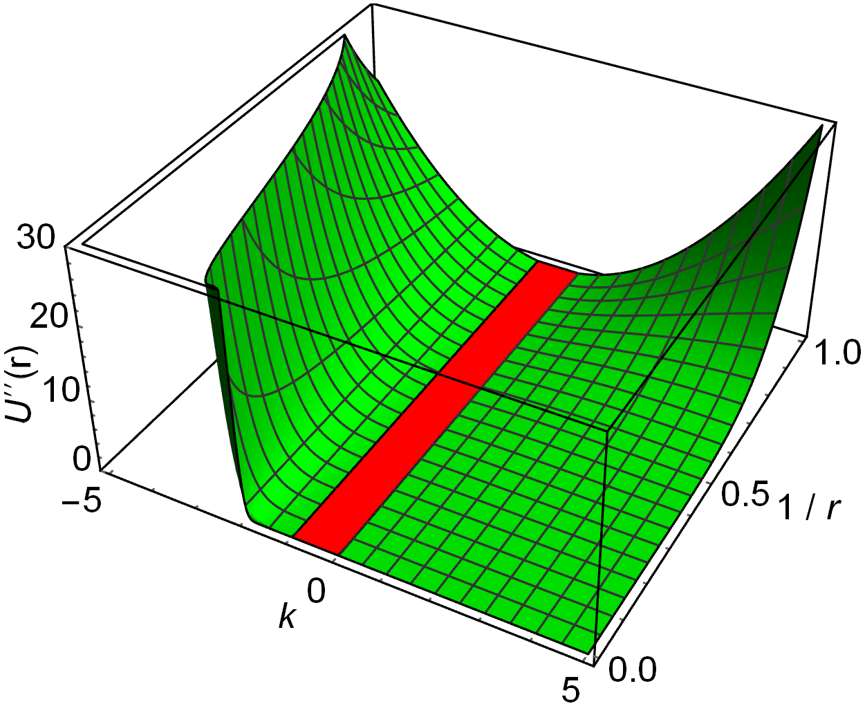
or that the potential must always fall with a decreasing rate, i.e. the potential $U(r)$ is strictly convex.

One can easily check that assumption (1.10) holds for Coulomb and dipole potentials, and all potentials of a form (see Fig. 1.1):

U(r)=\frac{C}{r^{k}},\quad k\not\in[-1;0].

(1.11)

However, in principle, a potential that does not satisfy such a condition could also be considered (such as the Pöschl-Teller potential [28] used in the description of ultracold atomic gases).

Refer to caption — Figure 1.1: Plot of $U^{\prime\prime}(r)$ for $U(r)=r^{-k}$ . Red region shows where the assumption (1.10) does not hold.

1.3.2 Motivation

The extended $t$ - $V$ model of fermions has one prominent feature that makes it of theoretical interest: its description is rather general, as the values of the potentials are not set. Therefore, it could describe an experimentally realisable one-dimensional system. With the recent nanotechnological advancements, it has become possible to engineer condensed matter systems using ultracold atoms in optical lattices [29, 30]. Additionally, because the system exhibits the Luttinger liquid–Mott insulator phase transition, it may be relevant to the experimental production and the operation of a one-dimensional Mott transistor. Finally, the investigation of the generalised $t$ - $V$ model may serve as a theoretical exercise that helps in the development and classification of usefulness of analytical and numerical methods that can deal with quantum systems with long-range interactions.

1.3.3 Formulation as a chain of spins

Every one-dimensional¹¹ 1 Although the same procedure can be used in higher-dimensional systems, the transformation will produce multiple non-local terms that require keeping track of many non-local quantum numbers. In one dimension all the non-local terms (see Eqs. (1.36–1.42)) include the number of particles $N$ , which is usually fixed during the setup of the system. system of spinless fermions can be formulated as an equivalent system of spins (spin-half). One way to do this is to use the Jordan-Wigner transformation [31], in which fermionic creation and annihilation operators are redefined as chains of spin operators,

\left\{\begin{array}[]{lll}c_{i}&=&e^{-i\pi\sum_{k=1}^{i-j}\sigma_{k}^{+}\sigma_{k}^{-}}\sigma_{i}^{-}\\ c_{i}^{{\dagger}}&=&e^{i\pi\sum_{k=1}^{i-j}\sigma_{k}^{+}\sigma_{k}^{-}}\sigma_{i}^{+}\end{array}\right.,

(1.12)

where $\sigma_{i}^{\pm}=(\sigma_{i}^{x}\pm i\sigma_{i}^{y})/2$ and $\sigma^{x},\sigma^{y},\sigma^{z}$ are the Pauli spin matrices:

\sigma^{x}=\left(\begin{array}[]{cc}0&1\\ 1&0\end{array}\right),\quad\sigma^{y}=\left(\begin{array}[]{cc}0&-i\\ i&0\end{array}\right),\quad\sigma^{z}=\left(\begin{array}[]{cc}1&0\\ 0&-1\end{array}\right).

(1.13)

We can see that

c_{i}=e^{-i\pi\sum_{k=1}^{i-j}\sigma_{k}^{+}\sigma_{k}^{-}}\sigma_{i}=\prod_{k=1}^{i-1}e^{\text{\scriptsize{$-i\pi\left(\begin{array}[]{cc}1&0\\ 0&0\end{array}\right)_{k}$}}}\sigma_{i}^{-}=\prod_{k=1}^{i-1}\left(\begin{array}[]{cc}-1&0\\ 0&1\end{array}\right)_{k}\sigma_{i}^{-}=\prod_{k=1}^{i-1}(-\sigma_{k}^{z})\sigma_{i}^{-},

(1.14)

and the transformation is simply

\left\{\begin{array}[]{lll}c_{i}&=&\prod_{k<i}(-\sigma_{k}^{z})\sigma_{i}^{-}\\ c_{i}^{{\dagger}}&=&\prod_{k<i}(-\sigma_{k}^{z})\sigma_{i}^{+}\end{array}\right..

(1.15)

Therefore one can calculate the following relations:

$\displaystyle c_{i}^{{\dagger}}c_{i+1}$	$\displaystyle=$	$\displaystyle\prod_{k<i}(-\sigma_{k}^{z})\sigma_{i}^{+}\prod_{l<i+1}(-\sigma_{l}^{z})\sigma_{i+1}^{-}$	(1.16)
	$\displaystyle=$	$\displaystyle(-\sigma_{1}^{z})\cdots(-\sigma_{i-1}^{z})\sigma_{i}^{+}(-\sigma_{1}^{z})\cdots(-\sigma_{i-1}^{z})(-\sigma_{i}^{z})\sigma_{i+1}^{-}$
	$\displaystyle=$	$\displaystyle-\sigma_{i}^{+}\sigma_{i}^{z}\sigma_{i+1}^{-}=-\left(\begin{array}[]{cc}0&1\\ 0&0\end{array}\right)_{i}\left(\begin{array}[]{cc}1&0\\ 0&-1\end{array}\right)_{i}\sigma_{i+1}^{-}$
	$\displaystyle=$	$\displaystyle\sigma_{i}^{+}\sigma_{i+1}^{-},$

$\displaystyle c_{i+1}^{{\dagger}}c_{i}$	$\displaystyle=$	$\displaystyle\prod_{k<i+1}(-\sigma_{k}^{z})\sigma_{i+1}^{+}\prod_{l<i}(-\sigma_{l}^{z})\sigma_{i}^{-}$	(1.22)
	$\displaystyle=$	$\displaystyle(-\sigma_{1}^{z})\cdots(-\sigma_{i-1}^{z})(-\sigma_{i}^{z})\sigma_{i+1}^{+}(-\sigma_{1}^{z})\cdots(-\sigma_{i-1}^{z})\sigma_{i}^{-}$
	$\displaystyle=$	$\displaystyle-\sigma_{i}^{z}\sigma_{i}^{-}\sigma_{i+1}^{+}=-\left(\begin{array}[]{cc}1&0\\ 0&-1\end{array}\right)_{i}\left(\begin{array}[]{cc}0&0\\ 1&0\end{array}\right)_{i}\sigma_{i+1}^{+}$
	$\displaystyle=$	$\displaystyle\sigma_{i+1}^{+}\sigma_{i}^{-},$

$\displaystyle n_{i}=c_{i}^{{\dagger}}c_{i}$	$\displaystyle=$	$\displaystyle\prod_{k<i}(-\sigma_{k}^{z})\sigma_{i}^{+}\prod_{l<i}(-\sigma_{l}^{z})\sigma_{i}^{-}$	(1.28)
	$\displaystyle=$	$\displaystyle(-\sigma_{1}^{z})\cdots(-\sigma_{i-1}^{z})\sigma_{i}^{+}(-\sigma_{1}^{z})\cdots(-\sigma_{i-1}^{z})\sigma_{i}^{-}$
	$\displaystyle=$	$\displaystyle\sigma_{i}^{+}\sigma_{i}^{-}=\left(\begin{array}[]{cc}0&1\\ 0&0\end{array}\right)_{i}\left(\begin{array}[]{cc}0&0\\ 1&0\end{array}\right)_{i}=\left(\begin{array}[]{cc}1&0\\ 0&0\end{array}\right)_{i}$
	$\displaystyle=$	$\displaystyle\mathbbm{P}_{i}^{{\uparrow}}=(1+\sigma^{z})/2,$

where $\mathbbm{P}_{i}^{{\uparrow}}$ is the projector operator to the spin-up subspace on site $i$ . In a periodic chain the hoppings over the boundary must be calculated independently,

$\displaystyle c_{L}^{{\dagger}}c_{1}$	$\displaystyle=$	$\displaystyle\prod_{k<L}(-\sigma_{k}^{z})\sigma_{L}^{+}\sigma_{1}^{-}=(-\sigma_{1}^{z})(-\sigma_{2}^{z})\cdots(-\sigma_{L-1}^{z})\sigma_{L}^{+}\sigma_{1}^{-}$	(1.36)
	$\displaystyle=$	$\displaystyle-\left(\begin{array}[]{cc}1&0\\ 0&-1\end{array}\right)_{1}\left(\begin{array}[]{cc}0&0\\ 1&0\end{array}\right)_{1}\prod_{k=2}^{L-1}(-\sigma_{k}^{z})\sigma_{L}^{+}=\sigma_{1}^{-}\sigma_{L}^{+}(-1)^{\sum_{k=2}^{L-1}n_{k}}$
	$\displaystyle=$	$\displaystyle\sigma_{1}^{-}\sigma_{L}^{+}(-1)^{N-1},$

$\displaystyle c_{1}^{{\dagger}}c_{L}$	$\displaystyle=$	$\displaystyle\sigma_{1}^{+}\prod_{k<L}(-\sigma_{k}^{z})\sigma_{L}^{-}=\sigma_{1}^{+}(-\sigma_{1}^{z})(-\sigma_{2}^{z})\cdots(-\sigma_{L-1}^{z})\sigma_{L}^{-}$	(1.42)
	$\displaystyle=$	$\displaystyle-\left(\begin{array}[]{cc}0&1\\ 0&0\end{array}\right)_{1}\left(\begin{array}[]{cc}1&0\\ 0&-1\end{array}\right)_{1}\prod_{k=2}^{L-1}(-\sigma_{k}^{z})\sigma_{L}^{-}$
	$\displaystyle=$	$\displaystyle\sigma_{1}^{+}\sigma_{L}^{-}(-1)^{N-1},$

where $N=\sum_{k}n_{k}$ is total number of particles. Terms describing hopping across the boundary can be treated as an effective flux²² 2 Since $(-1)^{N-1}=e^{i\pi(N-1)}$ , the flux is $\phi=\pi(N-1)/L$ . Therefore, in a system with an odd number of particles, there is no additional phase shift acquired while hopping, and in a system with even $N$ , there is a $-1=e^{i\pi}$ phase factor that needs to be included in the bosonic Hamiltonian. going through the chain.

The Hamiltonian (1.6) of the generalised $t$ - $V$ model becomes:

H=-t\sum_{i=1}^{L-1}(\sigma^{+}_{i}\sigma^{-}_{i+1})-t(-1)^{N-1}\sigma^{+}_{L}\sigma_{1}^{-}+\text{h.c.}+\sum_{i=1}^{L}\sum_{m=1}^{p}U_{m}\mathbbm{P}_{i}^{{\uparrow}}\mathbbm{P}^{{\uparrow}}_{i+m},

(1.48)

H=-t\sum_{i=1}^{L-1}(\sigma^{+}_{i}\sigma^{-}_{i+1})-t(-1)^{N-1}\sigma^{+}_{L}\sigma_{1}^{-}+\text{h.c.}+\frac{1}{4}\sum_{i=1}^{L}\sum_{m=1}^{p}U_{m}(1+\sigma^{z}_{i})(1+\sigma^{z}_{i+m}).

(1.49)

In case of $p=1$ , the model becomes equivalent to the XXZ Heisenberg model with background effective field, pierced by the magnetic flux.

1.3.4 Solution for the infinite potential

Here we summarise the solution of the generalised $t$ - $V$ model given by Gómez-Santos in Ref. [23]. This solution presents a very simple effective picture of the system, which nevertheless gives a lot of physical insight. Assumption (1.8) will hold during this consideration.

Firstly, let us consider the case of low energies, when any two fermions are never close enough to incur a potential energy penalty. The system loses some degrees of freedom, namely every particle effectively occupies $(p+1)$ sites. A particle can therefore be thought of as a fermion with a hard core or a hard rod occupying $(p+1)$ sites (see Fig. 1.2a). Thus, the system can be imagined as a chain of $N$ free fermions on

\tilde{L}=L-Np=L(1-Qp)

(1.50)

sites, where $Q=N/L$ is the density of the original system. The energy can be calculated to be simply:

E(\{\tilde{k}\})=-2t\sum_{i=1}^{N}\cos\tilde{k}_{i},\quad\tilde{k}_{i}=\frac{2\pi\tilde{n}_{i}}{\tilde{L}},\quad\tilde{n}_{i}\in\{0,\ldots,\tilde{L}-1\},

(1.51)

where $\{\tilde{k}\}$ denotes a set of all particle momenta $\tilde{k}_{i}$ in the system, and index $i$ labels the particles. The ground state energy density can be calculated by occupying the lowest-energy momentum space and taking the infinite volume limit:

\frac{E}{L}=-\frac{2t}{L}\sum_{\tilde{n}_{i}=-N/2}^{N/2}\cos\tilde{k}_{i}\quad\rightarrow\quad-2t\frac{1-Qp}{\pi}\sin\frac{\pi Q}{1-Qp}.

(1.52)

Let us now squeeze the system by removing empty sites one by one. We notice that there is a critical density (also called commensurate density), at which particles cannot move, otherwise it would cost them $U_{p}$ energy,

Q=1/(p+1).

(1.53)

At this density, the system is a Mott insulator and no fermion can move without inducing a huge energy penalty; hard rods fill the system completely (see Fig. 1.3). The energy is zero and all Luttinger liquid velocities also go to zero. By shaking this chain, one can create a charge-quasiparticle (an overlap of hard rods) moving through the system. A coherent superposition of such quasiparticles is called a charge-density-wave (CDW).

Squeezing this chain even more will necessarily add a potential energy $U_{p}$ . A quasiparticle that is created in the squeezing process will behave as a free particle in a tight-binding model (see Fig. 1.2b), with particle hopping by $p$ sites. If we shorten the chain even more, then either a new quasiparticle is created or the existing quasiparticle incorporates the new instability. However, the latter is forbidden by Assumption (1.8), and therefore, by squeezing the chain, we will always create new quasiparticles. Any number of those instabilities will behave like particles in a tight-binding chain, until there are so many instabilities they fill the whole system. We again reach an insulating density, this time at $Q=1/p$ .

A similar trend continues until the chain becomes half-filled. The rest of the insulating densities can easily be recovered using the particle-hole symmetry: a system with density $1-Q$ , $Q\in[0,0.5]$ exhibits the same physics as the system with density $Q$ . In short, the system is a Mott insulator at critical (commensurate) densities

Q=\frac{1}{m},\quad m=p+1,p,\ldots,M,

(1.54)

and is a Luttinger liquid at other, incommensurate densities. $M=\max(\lfloor p/2\rfloor+1,2)$ designates the last density $Q=1/M$ , where the potential $U_{\lfloor p/2\rfloor}$ does not contribute to the potential energy of the system³³ 3 Going beyond the density $Q=1/M$ may not be an issue if the potential energy decreases rapidly. In such a case, one can expect a Mott insulating phase at densities $Q=1/m,m=p+1,p,\ldots,2$ ..

The energy of the system in the high-energy subspace can be calculated by noticing that the system is now of the effective size $\tilde{L}=LQ$ and the number of quasiparticles is $\tilde{N}=L(1-Q\lfloor 1/Q\rfloor)$ . Similarly to Eq. (1.52), the energy in the infinite volume limit is:

\frac{E}{L}\rightarrow-2t\frac{Q}{\pi}\sin\pi\left(\frac{1}{Q}-\left\lfloor\frac{1}{Q}\right\rfloor\right).

(1.55)

Using Eqs. (1.52) and (1.55), the parameters of the Luttinger liquid were assessed to be:

v_{S}=\left\{\begin{array}[]{ll}\frac{2t}{1-Qp}\sin\frac{\pi Q}{1-Qp}&\operatorname{for}Q\leqslant\frac{1}{p+1},\\ \frac{2t}{Q}\left|\sin\frac{\pi}{Q}\right|&\operatorname{otherwise},\end{array}\right.\quad\operatorname{and}\quad K=\left\{\begin{array}[]{ll}\frac{1}{2}(1-Qp)^{2}&\operatorname{for}Q\leqslant\frac{1}{p+1},\\ \frac{1}{2}Q^{2}&\operatorname{otherwise}.\end{array}\right.

(1.56)

This simple yet rich solution gives us the energy spectrum shown in Fig. 1.4. The sound velocity $v_{S}$ is plotted in Fig. 1.5, which also shows the densities at which Luttinger liquid (blue) and Mott insulator (red) phases are formed. At the insulating density, all Luttinger liquid velocities go to zero.

Figure 1.4: Spectrum of the potential energy of the generalised

t

V

model in Gómez-Santos’s solution. The scale is logarithmic and it is assumed that

0\ll U_{p}\ll U_{p-1}\ll\cdots

and that condition (1.8) holds.

Figure 1.5: Sound velocity

v_{S}

as a function of density

Q

. Example for

p=4

1.3.5 Non-Bethe ansatz solution for the system with nearest-neighbour interactions

Here we summarise method alternative to the Bethe ansatz of solving the $t$ - $V$ model ( $p=1$ ). The method was developed by Dias in Ref. [32]. The main motivation behind developing a different method is that, although the Bethe ansatz is a very powerful tool, it is still based on an educated guess and therefore misses a lot of the underlying physics.

Firstly, the kinetic part of the Hamiltonian (1.6) is assumed to be much smaller than the potential ( $t\ll U_{1}$ ). If $t=0$ , the Hilbert space consists of degenerate subspaces with states of constant values of $\sum_{i=1}^{L}n_{i}n_{i+1}$ . For $t\ll U_{1}$ this degeneracy is lifted, but in order to calculate the eigenvalues up to the first perturbation order, we can diagonalise the Hamiltonian within each of the degenerate subspaces. The projected Hamiltonian (1.6) is:

	$\displaystyle H$	$\displaystyle=$	$\displaystyle-t\sum_{i=1}^{L}\left((1-n_{i-1})c^{{\dagger}}_{i}c_{i+1}(1-n_{i+2})+\text{h.c.}\right)$		(1.57)
		$\displaystyle-$	$\displaystyle t\sum_{i=1}^{L}\left(n_{i-1}c^{{\dagger}}_{i}c_{i+1}n_{i+2}+\text{h.c.}\right)+U_{1}\sum_{i=1}^{L}n_{i}n_{i+1}.$		(1.57)

Now we proceed by observing which hoppings are allowed and which are forbidden in the projected Hamiltonian. The operators $(1-n_{i-1}),(1-n_{i+2}),n_{i-1}$ and $n_{i+2}$ ensure that the hopping between sites $i$ and $(i+1)$ is only possible, if sites $(i-1)$ and $(i+2)$ are either both occupied or both empty. Table 1.1 shows all possible hoppings and chains in which hoppings should not be allowed.

Hopping	Decomposition into two-site chains	Mapping
$({\circ}{\circ}{\bullet}{\circ})$	${\color[rgb]{0,0.4375,0.7539}({\circ}{\circ})}{\color[rgb]{0.4609,0.5742,0.2344}({\circ}{\bullet})}({\bullet}{\circ})$	${\downarrow}{\odot}$
$({\circ}{\bullet}{\circ}{\circ})$	${\color[rgb]{0.4609,0.5742,0.2344}({\circ}{\bullet})}({\bullet}{\circ}){\color[rgb]{0,0.4375,0.7539}({\circ}{\circ})}$	${\odot}{\downarrow}$
$({\bullet}{\circ}{\bullet}{\bullet})$	$({\bullet}{\circ}){\color[rgb]{0.4609,0.5742,0.2344}({\circ}{\bullet})}{\color[rgb]{0.7539,0.3125,0.3008}({\bullet}{\bullet})}$	${\odot}{\uparrow}$
$({\bullet}{\bullet}{\circ}{\bullet})$	${\color[rgb]{0.7539,0.3125,0.3008}({\bullet}{\bullet})}({\bullet}{\circ}){\color[rgb]{0.4609,0.5742,0.2344}({\circ}{\bullet})}$	${\uparrow}{\odot}$
No hoppings should be allowed
$({\circ}{\circ}{\bullet}{\bullet})$	${\color[rgb]{0,0.4375,0.7539}({\circ}{\circ})}{\color[rgb]{0.4609,0.5742,0.2344}({\circ}{\bullet})}{\color[rgb]{0.7539,0.3125,0.3008}({\bullet}{\bullet})}$	${\downarrow}\cancel{{\odot}}{\uparrow}$
$({\circ}{\bullet}{\circ}{\bullet})$	${\color[rgb]{0.4609,0.5742,0.2344}({\circ}{\bullet})}({\bullet}{\circ}){\color[rgb]{0.4609,0.5742,0.2344}({\circ}{\bullet})}$	${\odot}{\odot}$
$({\bullet}{\circ}{\bullet}{\circ})$	$({\bullet}{\circ}){\color[rgb]{0.4609,0.5742,0.2344}({\circ}{\bullet})}({\bullet}{\circ})$	${\odot}$
$({\bullet}{\bullet}{\circ}{\circ})$	${\color[rgb]{0.7539,0.3125,0.3008}({\bullet}{\bullet})}({\bullet}{\circ}){\color[rgb]{0,0.4375,0.7539}({\circ}{\circ})}$	${\uparrow}{\downarrow}$

Table 1.1: All possible hoppings from the second to the third site in a four-site chain in a

p=1

system. Two-site chains are mapped according to Eq. (1.58).

In order to simplify the problem, we now decompose each four-site chain into two-site chains. The two-site chains are then named according to the following mapping:

$\displaystyle\hskip 60.00009pt{\color[rgb]{0.7539,0.3125,0.3008}({\bullet}{\bullet})}$	$\displaystyle=$	$\displaystyle{\uparrow}\quad\text{(occupied site, spin-up)}$	(1.58)
$\displaystyle{\color[rgb]{0,0.4375,0.7539}({\circ}{\circ})}$	$\displaystyle=$	$\displaystyle{\downarrow}\quad\text{(occupied site, spin-down)}$
$\displaystyle{\color[rgb]{0.4609,0.5742,0.2344}({\circ}{\bullet})}$	$\displaystyle=$	$\displaystyle{\odot}\hskip 7.5pt\text{(empty site).}$

Notice that in order to make the mapping unambiguous, the $({\bullet}{\circ})$ chain is always discarded during the mapping. To maintain the properties of the system, the mapping must also preserve which states are allowed to hop and which are forbidden to hop. The spin-up occupied site ${\uparrow}$ is only allowed to hop with the empty site ${\odot}$ . Similarly, the spin-down occupied site ${\downarrow}$ can only hop with the empty site ${\odot}$ . However, no other hoppings are allowed.

Using the rules above, we notice that there is one four-site chain, which introduces a problem: in $({\circ}{\circ}{\bullet}{\bullet})$ chain the hopping should not be possible, but after the mapping the chain becomes $({\downarrow}{\odot}{\uparrow})$ , in which the empty site ${\odot}$ can either hop with the ${\downarrow}$ site or the ${\uparrow}$ site. We notice that this problem is due to the two-site chain $({\circ}{\bullet})$ acting as a domain wall between empty sites $\cdots{\circ}{\circ}\cdots$ and occupied sites $\cdots{\bullet}{\bullet}\cdots$ . Therefore, in order to recover unambiguity of the mapping, we are forced to remove any chain $({\circ}{\bullet})$ , which acts as a domain wall between sites ${\downarrow}$ and ${\uparrow}$ .

Example. A chain (with periodic boundary conditions)

{\circ}{\circ}{\circ}{\circ}{\bullet}{\bullet}{\bullet}{\circ}{\circ}{\circ}

(1.59) can be decomposed into two-site chains

{\color[rgb]{0,0.4375,0.7539}({\circ}{\circ})}{\color[rgb]{0,0.4375,0.7539}({\circ}{\circ})}{\color[rgb]{0,0.4375,0.7539}({\circ}{\circ})}{\color[rgb]{0.4609,0.5742,0.2344}({\circ}{\bullet})}{\color[rgb]{0.7539,0.3125,0.3008}({\bullet}{\bullet})}{\color[rgb]{0.7539,0.3125,0.3008}({\bullet}{\bullet})}({\bullet}{\circ}){\color[rgb]{0,0.4375,0.7539}({\circ}{\circ})}{\color[rgb]{0,0.4375,0.7539}({\circ}{\circ})}{\color[rgb]{0,0.4375,0.7539}({\circ}{\circ})}

(1.60) and mapped into

{\downarrow}{\downarrow}{\downarrow}\cancel{{\odot}}{\uparrow}{\uparrow}{\downarrow}{\downarrow}{\downarrow}.

(1.61) Notice that because the empty site

{\odot}

was acting as a domain wall, it must be removed during the mapping.

Example. A chain

{\circ}{\circ}{\circ}{\circ}{\bullet}{\circ}{\bullet}{\circ}{\bullet}{\bullet}{\bullet}{\circ}{\circ}{\circ}

(1.62) can be decomposed into the following two-site chains

{\color[rgb]{0,0.4375,0.7539}({\circ}{\circ})}{\color[rgb]{0,0.4375,0.7539}({\circ}{\circ})}{\color[rgb]{0,0.4375,0.7539}({\circ}{\circ})}{\color[rgb]{0.4609,0.5742,0.2344}({\circ}{\bullet})}({\bullet}{\circ}){\color[rgb]{0.4609,0.5742,0.2344}({\circ}{\bullet})}({\bullet}{\circ}){\color[rgb]{0.4609,0.5742,0.2344}({\circ}{\bullet})}{\color[rgb]{0.7539,0.3125,0.3008}({\bullet}{\bullet})}{\color[rgb]{0.7539,0.3125,0.3008}({\bullet}{\bullet})}({\bullet}{\circ}){\color[rgb]{0,0.4375,0.7539}({\circ}{\circ})}{\color[rgb]{0,0.4375,0.7539}({\circ}{\circ})}{\color[rgb]{0,0.4375,0.7539}({\circ}{\circ})}

(1.63) and mapped into

{\downarrow}{\downarrow}{\downarrow}{\odot}{\odot}\cancel{{\odot}}{\uparrow}{\uparrow}{\downarrow}{\downarrow}{\downarrow}.

(1.64) Again, one of the empty sites

{\odot}

was acting as a domain wall between

{\downarrow}

and

{\uparrow}

, and therefore it must be removed during the mapping.

So, if in the system there is a spin down ${\downarrow}$ state followed by empty site(s) ${\odot}$ and a spin up ${\uparrow}$ , one of the empty sites needs to be removed, because it acts as a domain wall:

\cdots{\downarrow}{\odot}\cdots{\odot}\cancel{{\odot}}{\uparrow}\cdots.

(1.65)

Finally, let us consider a periodic system, which begins with two-site chain that will be discarded during the mapping (it can be either a $({\bullet}{\circ})$ chain or a $({\circ}{\bullet})$ that acts as a domain wall). Notice that the mapping is no longer unique: translating the system by one site to the left will result in a system with the same mapping. To mend this situation, we have to translate the system first, so that the first two-site chain can be mapped.

Example. The periodic system

{\bullet}{\circ}{\bullet}{\circ}{\circ}{\bullet}{\bullet}

(1.66) starts with a

({\bullet}{\circ})

chain. Therefore, we use a translation operator

T

T({\circ}{\bullet}{\circ}{\circ}{\bullet}{\bullet}{\bullet}),

(1.67) and now we can map the system:

T\left({\odot}{\downarrow}\cancel{{\odot}}{\uparrow}{\uparrow}\right).

(1.68)

Notice that if before the mapping the system has $L$ sites, after the mapping the system has length:

\tilde{L}=L-N_{{\odot}}-2N_{\operatorname{DW}},

(1.69)

where $N_{{\odot}}$ is the number of mapped empty sites ${\odot}$ and $N_{\operatorname{DW}}$ is the number of empty sites acting as domain walls $\cancel{{\odot}}$ . The number of fermions after the mapping is

\tilde{N}=N_{{\uparrow}}+N_{{\downarrow}}.

(1.70)

If the initial states were designated by positions $a_{i}$ of the fermions,

|a_{1},\ldots,a_{N}\rangle=\prod_{i=1}^{N}c^{{\dagger}}_{a_{i}}|0\rangle,

(1.71)

then in the mapped system, the states will be designated by positions of fermions, $\tilde{a}_{i}$ , and their spins, $\sigma_{i}$ ,

|\tilde{a}_{1},\ldots,\tilde{a}_{\tilde{N}};\sigma_{1},\ldots,\sigma_{\tilde{N}}\rangle=\prod_{i=1}^{\tilde{N}}\tilde{c}^{{\dagger}}_{\tilde{a}_{i}\sigma_{i}}|\tilde{0}\rangle.

(1.72)

Example. One can map

{\bullet}{\bullet}{\circ}{\circ}{\bullet}{\circ}{\bullet}{\circ}{\bullet}

(1.73) into

{\uparrow}{\downarrow}{\odot}{\odot}\cancel{{\odot}}{\uparrow}.

(1.74) A spinless chain of

N=5

fermions on

L=9

sites is therefore mapped into a spinful chain of

\tilde{N}=3

fermions on

\tilde{L}=5

sites. The initial state is

|1,2,5,7,9\rangle

(1.75) and after mapping it becomes

|\tilde{1},\tilde{2},\tilde{5};{\uparrow},{\downarrow},{\uparrow}\rangle.

(1.76)

Example. The system from Eq. (1.68) corresponds to the following state:

|1,3,6,7\rangle\longrightarrow T|\tilde{2},\tilde{3},\tilde{4};{\downarrow},{\uparrow},{\uparrow}\rangle.

(1.77)

Now, we create new states that are invariant by translation and have total momentum $P$ :

|\{\tilde{a}\},\{\sigma\},P\rangle=|\{a\},P\rangle=\frac{1}{\sqrt{L}}\sum_{j=1}^{L}e^{iPj}T^{j-1}|\{a\}\rangle.

(1.78)

Due to the requirement that the first two-site chain must be possible to map (see the example state from Eq. (1.77)), the Hamiltonian elements that correspond to jumps $\tilde{1}\rightarrow\tilde{L}$ and $\tilde{2}\rightarrow\tilde{1}$ , will give additional $e^{\pm iP}$ factors, that can be incorporated into the hopping constant $t$ . A detailed table of all these elements is shown in Ref. [32] p. 7795. The Hamiltonian $H_{1}=H-U_{1}N_{{\uparrow}}$ becomes

H_{1}(P)=-\sum_{\tilde{i},\sigma}t_{\tilde{i}\sigma}(1-n_{\tilde{i}\sigma})\tilde{c}^{{\dagger}}_{\tilde{i}\sigma}\tilde{c}_{\tilde{i}+1,\sigma}(1-n_{\tilde{i}+1,\sigma})+\text{h.c.},

(1.79)

with $t_{\tilde{L}{\uparrow}}=t(-1)^{L-N},t_{\tilde{L}{\downarrow}}=te^{iP}(-1)^{L-N},t_{\tilde{1}{\uparrow}}=te^{\sigma_{\tilde{N}}iP}$ and $t_{\tilde{i}\sigma}=t$ otherwise. This is the Hamiltonian of a $U\rightarrow\infty$ Hubbard chain pierced by a magnetic flux⁴⁴ 4 The Hubbard model is a model of spinful fermions with the following Hamiltonian: $H=-t\sum_{\langle i,j\rangle,\sigma}\left(c^{{\dagger}}_{i,\sigma}c_{j,\sigma}+\text{h.c.}\right)+U\sum_{i=1}^{N}n_{i{\uparrow}}n_{i{\downarrow}}.$ (1.80) Notice that the sites can be doubly occupied, unless $U\rightarrow\infty$ ..

Now, we consider a subspace of states in the Hamiltonian, with the same configuration of $\{\sigma\}$ :

H_{1}(P,\{\sigma\})=-t\sum_{\tilde{i}\neq\tilde{L}}\tilde{c}_{\tilde{i}+1}^{{\dagger}}\tilde{c}_{\tilde{i}}-t_{\tilde{1}\sigma_{1}}\tilde{c}^{{\dagger}}_{\tilde{1}}\tilde{c}_{\tilde{2}}-t_{\tilde{L}\sigma_{1}}\tilde{c}^{{\dagger}}_{\tilde{L}}\tilde{c}_{\tilde{1}}Q+\text{h.c.},

(1.81)

where $Q$ is the cyclic spin permutation operator, that permutes $\{\sigma\}$ in a state. We will now do the following gauge transformation,

\forall_{\tilde{a}_{1}\geqslant 2}\kern 5.0pt|\tilde{a}_{1},\ldots,\tilde{a}_{\tilde{N}};{\uparrow},\ldots,\sigma_{\tilde{N}}\rangle\rightarrow e^{\sigma_{\tilde{N}}iP}|\tilde{a}_{1},\ldots,\tilde{a}_{\tilde{N}};{\uparrow},\ldots,\sigma_{\tilde{N}}\rangle.

(1.82)

The Hamiltonian (1.81) in the subspace of the same spin configuration will now have the same form as in Eq. (1.79), but with $t_{\tilde{L}\sigma}=(-1)^{L-N}te^{\frac{1}{2}(1+\sigma_{1}\cdot\sigma_{\tilde{N}})iP}$ and $t_{\tilde{i}\sigma}=t$ otherwise. If we now hop a fermion across the boundary, it will induce a cyclic permutation of $\{\sigma\}$ with the same phase factor that is included in $t_{\tilde{L}\sigma}$ . Now, we want to define states that remain invariant under such cyclic permutations:

Q_{\{\sigma\}}\left(\sum_{i=1}^{r_{\alpha_{c}}}\tilde{a}_{i}Q^{i}|\{\sigma\}\rangle\right)=e^{i\phi^{\prime}/r_{\alpha_{c}}}\left(\sum_{i=1}^{r_{\alpha_{c}}}\tilde{a}_{i}Q^{i}|\{\sigma\}\rangle\right),

(1.83)

where $r_{\alpha_{c}}$ is the periodicity of the spins $\{\sigma\}$ (notice that $r_{\alpha_{c}}$ must be a divisor of $\tilde{N}$ ), $\alpha_{c}$ is a number designating a possible spin configuration, $Q_{\{\sigma\}}$ is defined by

Q_{\{\sigma\}}|\sigma_{1},\ldots,\sigma_{\tilde{N}}\rangle=\frac{t_{\tilde{L}\sigma}}{t}Q|\sigma_{1},\ldots,\sigma_{\tilde{N}}\rangle,

(1.84)

and $\phi^{\prime}$ is the effective flux through the newly redefined system.

Example. Spin periodicity of some example systems:

\displaystyle({\odot}{\uparrow}{\odot}{\uparrow}{\uparrow})\rightarrow\hskip 62.00006pt|\tilde{2},\tilde{4},\tilde{5};{\uparrow},{\uparrow},{\uparrow}\rangle

\displaystyle\rightarrow

\displaystyle r_{\alpha_{c}}=1,

(1.85)

\displaystyle\left({\downarrow}{\downarrow}{\odot}\cancel{{\odot}}{\uparrow}{\odot}{\downarrow}{\odot}{\odot}{\downarrow}\cancel{{\odot}}{\uparrow}\right)\rightarrow|\tilde{1},\tilde{2},\tilde{4},\tilde{6},\tilde{9},\widetilde{10};{\downarrow},{\downarrow},{\uparrow},{\downarrow},{\downarrow},{\uparrow}\rangle

\displaystyle\rightarrow

\displaystyle r_{\alpha_{c}}=3,

\displaystyle T\left({\odot}{\downarrow}\cancel{{\odot}}{\uparrow}{\uparrow}\right)\rightarrow\hskip 54.00002ptT|\tilde{2},\tilde{3},\tilde{4};{\downarrow},{\uparrow},{\uparrow}\rangle

\displaystyle\rightarrow

\displaystyle r_{\alpha_{c}}=3.

We want the system to become a one-particle tight-binding model with $r_{\alpha_{c}}$ sites and hopping constant $te^{\frac{1}{2}(1+\sigma_{1}\cdot\sigma_{\tilde{N}})iP}$ and with one-particle states defined as

Q^{i-1}|\{\sigma\}\rangle\equiv|i\rangle.

(1.86)

To achieve all that, the following gauge transformation is needed,

te^{\frac{1}{2}(1+\sigma_{1}\cdot\sigma_{\tilde{N}})iP}\rightarrow te^{i\phi_{1}/r_{\alpha_{c}}},

(1.87)

where the total flux $\phi_{1}$ through this tight-binding chain is found to be

\phi_{1}=r_{\alpha_{c}}\frac{\tilde{N}-2N_{\operatorname{DW}}}{\tilde{N}}P,

(1.88)

where $N_{\operatorname{DW}}$ is the number of $({\circ}{\bullet})$ chains that are treated as domain walls ( $\cancel{{\odot}}$ ). The chain now is a Hubbard model with flux $\phi_{1}$ and its eigenstates are Bloch states $|\alpha_{c},q_{c}\rangle$ , where $q_{c}$ is a momentum of the Bloch state in the cyclic permutations of the $\{\sigma\}$ configuration,

q_{c}=\frac{2\pi n_{\alpha_{c}}}{r_{\alpha_{c}}},\quad n_{\alpha_{c}}=0,\ldots,r_{\alpha_{c}}-1.

(1.89)

Following Ref. [33], the energy (for odd $N$ ) is given by

E(\{\tilde{k}\},q_{c},P)=-2t\sum_{i=1}^{\tilde{N}}\cos\left(\tilde{k}_{i}+\alpha\frac{P}{\tilde{L}}+\frac{q_{c}}{\tilde{L}}\right),

(1.90)

with $\alpha=\frac{2\tilde{L}-L}{\tilde{N}}=\frac{\tilde{N}-2N_{\operatorname{DW}}}{\tilde{N}}$ , while for even $N$ there is a $+\frac{\pi}{\tilde{L}}$ correction under the cosine. There is also the following condition on the total momentum that needs to be satisfied:

P\frac{L}{\tilde{L}}=\sum_{i=1}^{\tilde{N}}\tilde{k}_{i}+\tilde{N}\frac{q_{c}}{\tilde{L}}\quad(\operatorname{mod}2\pi).

(1.91)

To calculate the ground state energy, we assume that there are no $({\bullet}{\bullet})$ chains, and thus no spin-down particles in the mapped system. Then, the spin periodicity is $r_{\alpha_{c}}=1$ , and thus $q_{c}=0$ . Particles occupy the lowest momentum states, and thus $\sum_{i}\tilde{k}_{i}=0$ . The ground state energy can be therefore evaluated to be:

E=\left\{\begin{array}[]{ll}-2t\frac{\sin\frac{\pi N}{\tilde{L}}}{\sin\frac{\pi}{\tilde{L}}}&\operatorname{for}\operatorname{odd}N,\\ -2t\frac{\sin\frac{\pi N}{\tilde{L}}}{\sin\frac{\pi}{\tilde{L}}}\cos\frac{\pi}{L}&\operatorname{for}\operatorname{even}N.\end{array}\right.

(1.92)

In short, by using the mapping (1.58), one can change the spinless system into a spinful chain with magnetic flux. Then, by alternating gauge transformations and redefinition of states, so that the new states are invariant by translation (in a mapped position space and mapped spin space), we obtain a simple Hubbard model with a known solution.

We would like to use a similar method to solve the generalised ( $p\neq 1$ ) $t$ - $V$ model of fermions, since this method provides a more complete description of the system than, for example, Bethe ansatz. In contrast to Gómez-Santos’ solution summarised in Chapter 1.3.4, this method also considers domains of high energy, that can be present in the system. For example, the chain $({\circ}{\circ}{\bullet}{\bullet}{\bullet}{\circ}{\circ}{\circ})$ is never considered in Gómez-Santos’ solution, but is present in Dias’ solution. Thus, we could not only achieve more physical understanding, but also include the full spectrum of possible states.

Secondly, the ground state behaviour described in the Gómez-Santos’ solution is only considered with the infinite volume limit: comparing Eqs. (1.52) and (1.92) shows a discrepancy, but one can see that they match if $L\rightarrow\infty$ :

\lim_{L\rightarrow\infty}E^{\text{Dias}}=E^{\text{G{\'{o}}mez-Santos}}_{p=1}.

(1.93)

Chapter 2 Solving the generalised $t$ - $V$ model

2.1 Finite volumes with any interaction range and with infinite potential

2.1.1 Low-energy subspace

Similarly to the solution presented in Chapter 1.3.5, we can introduce a mapping of the original states into a system of lower length. Let us consider a small subchain of $p+1$ consecutive sites. Of course there are $2^{p+1}$ possible configurations of such a chain. In the low-energy subspace though, there are no $(p+1)$ -site subchains which include more than one particle, because otherwise there would be energy penalty $\geqslant U_{p}$ . Thus we are left with the following possible (one-particle and no-particle) chains:

({\bullet}{\circ}{\circ}\cdots{\circ});({\circ}{\bullet}{\circ}\cdots{\circ});({\circ}{\circ}{\bullet}\cdots{\circ});\cdots;({\circ}{\circ}{\circ}\cdots{\bullet});({\circ}{\circ}{\circ}\cdots{\circ}).

(2.1)

However, to have a unique one-to-one mapping (similarly to mapping (1.58)), we forget about all other subchains except $({\circ}\cdots{\circ}{\circ}{\bullet})$ and $({\circ}{\circ}{\circ}\cdots{\circ})$ . Therefore, we are left with only two subchains, which we will name for the sake of simplicity

	$\displaystyle({\circ}\cdots{\circ}{\circ}{\bullet})$	$\displaystyle=$	$\displaystyle{\circledast}\quad(\operatorname{occupied}\operatorname{site}),$		(2.2)
	$\displaystyle({\circ}\cdots{\circ}{\circ}{\circ})$	$\displaystyle=$	$\displaystyle{\odot}\quad(\operatorname{empty}\operatorname{site}).$

Notice that in the whole system with $N$ particles, there are exactly $\tilde{L}=L-Np$ subchains like these and thus the size of the mapped system is $\tilde{L}$ .

2.1.1.1 One particle

Of course, with only one particle the solution is quite simple and we expect to have a free particle that can propagate through the system with momentum $k=\frac{2\pi n}{L},n=0,\ldots,L-1$ . However, this case serves as an example of how to proceed in the many-particle case.

Firstly, a state with a particle on site $i$ in the original chain can be written as:

|i\rangle=c_{i}^{{\dagger}}|0\rangle.

(2.3)

Using mapping (2.2), we can rename those states to:

|\tilde{i}\rangle=c_{i+p}^{{\dagger}}|0\rangle=\tilde{c}_{\tilde{i}}^{{\dagger}}|\tilde{0}\rangle,

(2.4)

where $\tilde{c}_{\tilde{i}}^{{\dagger}}$ is the creation operator of subchain ${\circledast}$ and $|\tilde{0}\rangle$ is the “empty space” state ${\odot}{\odot}{\odot}\cdots$ of length $\tilde{L}=L-p$ . However, some states $|i\rangle$ are not included in this new set, namely states for $i\leq p$ . We can use translation operator $T$ to define them:

c_{i}^{{\dagger}}|0\rangle=T^{-p+i-1}c_{p+1}^{{\dagger}}|0\rangle=T^{-p+i-1}\tilde{c}_{\tilde{1}}^{{\dagger}}|\tilde{0}\rangle\quad\operatorname{for}i\leq p.

(2.5)

The Hamiltonian in the new notation is therefore

$\displaystyle\frac{H}{-t}$	$\displaystyle=$	$\displaystyle\sum_{i=p+1}^{L-1}c_{\tilde{i}}^{{\dagger}}c_{\tilde{i}+1}+c_{L}^{{\dagger}}c_{1}+c_{1}^{{\dagger}}c_{2}+\cdots+c_{p}^{{\dagger}}c_{p+1}+\text{h.c.}$	(2.6)
	$\displaystyle=$	$\displaystyle\sum_{\tilde{i}=\tilde{1}}^{\tilde{L}-1}\tilde{c}_{\tilde{i}}^{{\dagger}}\tilde{c}_{\tilde{i}+1}+\tilde{c}_{\tilde{L}}^{{\dagger}}\tilde{c}_{\tilde{1}}T^{p}+T^{-p}\tilde{c}_{\tilde{1}}^{{\dagger}}\tilde{c}_{\tilde{1}}T^{p-1}+\cdots+T^{-1}\tilde{c}_{\tilde{1}}^{{\dagger}}\tilde{c}_{\tilde{1}}+\text{h.c.}$
	$\displaystyle=$	$\displaystyle\sum_{\tilde{i}=\tilde{1}}^{\tilde{L}-1}\tilde{c}_{\tilde{i}}^{{\dagger}}\tilde{c}_{\tilde{i}+1}+\tilde{c}_{\tilde{L}}^{{\dagger}}\tilde{c}_{\tilde{1}}T^{p}+\sum_{m=1}^{p}T^{-p+m-1}\tilde{c}_{\tilde{1}}^{{\dagger}}\tilde{c}_{\tilde{1}}T^{p-m}+\text{h.c.}$

Following Dias [32], we introduce an over-complete set of states invariant by translation and with momentum $k$ :

|\tilde{i},k\rangle=\frac{1}{\sqrt{L}}\sum_{j=1}^{L}e^{ikj}T^{j-1}|\tilde{i}\rangle.

(2.7)

Creation and annihilation operators of these states will be designated as $\tilde{c}_{\tilde{i},k}^{{\dagger}}$ and $\tilde{c}_{\tilde{i},k}$ respectively. The Hamiltonian becomes:

$\displaystyle\frac{H}{-t}$	$\displaystyle=$	$\displaystyle\sum_{k}\left(\sum_{\tilde{i}=\tilde{1}}^{\tilde{L}-1}\tilde{c}_{\tilde{i},k}^{{\dagger}}\tilde{c}_{\tilde{i}+1,k}+e^{ikp}\tilde{c}_{\tilde{L},k}^{{\dagger}}\tilde{c}_{\tilde{1},k}+\sum_{m=1}^{p}e^{-ik}\tilde{c}_{\tilde{1},k}^{{\dagger}}\tilde{c}_{\tilde{1},k}+\text{h.c.}\right)$	(2.8)
	$\displaystyle=$	$\displaystyle\sum_{k}\left(\sum_{\tilde{i}=\tilde{1}}^{\tilde{L}-1}\tilde{c}_{\tilde{i},k}^{{\dagger}}\tilde{c}_{\tilde{i}+1,k}+e^{ikp}\tilde{c}_{\tilde{L},k}^{{\dagger}}\tilde{c}_{\tilde{1},k}+\text{h.c.}+(2p\cos k)\tilde{c}_{\tilde{1},k}^{{\dagger}}\tilde{c}_{\tilde{1},k}\right)$
	$\displaystyle=$	$\displaystyle\sum_{k}\left(\sum_{\tilde{i}=\tilde{1}}^{\tilde{L}-1}\tilde{c}_{\tilde{i},k}^{{\dagger}}\tilde{c}_{\tilde{i}+1,k}+e^{ikp}\tilde{c}_{\tilde{L},k}^{{\dagger}}\tilde{c}_{\tilde{1},k}+\text{h.c.}\right).$

This is the Hamiltonian of a tight-binding model with fictitious flux $e^{ikp}$ . Eigenvalues are given by

E(\tilde{k},k)=-2t\cos\left(\tilde{k}-\frac{kp}{\tilde{L}}\right),

(2.9)

with condition

\tilde{k}=k\frac{L}{\tilde{L}}\quad(\operatorname{mod}2\pi).

(2.10)

This final condition comes from the fact that eigenstates of Hamiltonian (2.8) are combinations of the over-complete set of states from Eq. (2.7) and are non-zero only if Eq. (2.10) is fulfilled. Finally, combining condition (2.10) and equation (2.9) for the energy, we recover the expected value for the energy of a particle with momentum $k$ :

E(k)=-2t\cos k.

(2.11)

2.1.1.2 Many particle case

Let us now consider a general case of $N$ particles. We must remember that any $(p+1)$ subchains must contain at most one particle. A specific realisation of our system can be written as:

|a_{1},\ldots,a_{N}\rangle=\prod_{i=1}^{N}c^{{\dagger}}_{a_{i}}|0\rangle,

(2.12)

where $\{a_{i}\}$ are the consecutive positions of particles in our system, $a_{i}\in\{1,\ldots,L\}$ . There is an additional condition on the first number, $a_{1}>p$ . This means that the first particle cannot occupy sites from $1$ to $p$ and thus there are states not included in this naming. However, we can represent them using the translation operator $T$ :

$\displaystyle c_{1}\prod_{i=2}^{N}c^{{\dagger}}_{a_{i}}\|0\rangle$	$\displaystyle=$	$\displaystyle T^{-p}\|p+1,a_{2}+p,\ldots,a_{N}+p\rangle,$	(2.13)
$\displaystyle c_{2}\prod_{i=2}^{N}c^{{\dagger}}_{a_{i}}\|0\rangle$	$\displaystyle=$	$\displaystyle T^{-p+1}\|p+1,a_{2}+p-1,\ldots,a_{N}+p-1\rangle,$
$\displaystyle c_{p}\prod_{i=2}^{N}c^{{\dagger}}_{a_{i}}\|0\rangle$	$\displaystyle=$	$\displaystyle T^{-1}\|p+1,a_{2}+1,\ldots,a_{N}+1\rangle.$

Now, we will use mapping (2.2) and rename states (2.12) to

|\tilde{a}_{1},\ldots,\tilde{a}_{N}\rangle=\prod_{i=1}^{N}\tilde{c}^{{\dagger}}_{\tilde{a}_{i}}|\tilde{0}\rangle,

(2.14)

where $\{\tilde{a}_{i}\}$ are now consecutive positions of subchains ${\circledast}$ , $|\tilde{0}\rangle$ is the “empty” system ${\odot}{\odot}{\odot}\cdots$ of size $\tilde{L}=L-Np$ and $\tilde{c}^{{\dagger}}_{\tilde{a}_{i}}$ creates a subchain ${\circledast}$ at position $\tilde{a}_{i}$ . We can now create a state invariant by translation, with momentum $P=\frac{2\pi n}{L},n=0,\ldots,L-1$ :

|\tilde{a}_{1},\ldots,\tilde{a}_{N},P\rangle=\frac{1}{\sqrt{L}}\sum_{j=1}^{L}e^{iPj}T^{j-1}|\tilde{a}_{1},\ldots,\tilde{a}_{N}\rangle.

(2.15)

The creation and annihilation operators of the new states will be designated as $\tilde{c}_{\tilde{i},P}^{{\dagger}}$ and $\tilde{c}_{\tilde{i}+1,P}$ . The Hamiltonian between the new states is thus:

\frac{H(P)}{-t}=\sum_{P}\left(\sum_{\tilde{i}\neq\tilde{L}}\tilde{c}_{\tilde{i},P}^{{\dagger}}\tilde{c}_{\tilde{i}+1,P}+e^{ipP}\tilde{c}_{\tilde{1},P}^{{\dagger}}\tilde{c}_{\tilde{L},P}\right)+\text{h.c.}

(2.16)

This is a Hamiltonian of a tight-binding chain with $\tilde{L}$ sites and fictitious flux $pP$ . The energy spectrum is given by:

E(\{\tilde{k}_{i}\},P)=-2t\sum_{i=1}^{N}\cos\left(\tilde{k}_{i}-\frac{pP}{\tilde{L}}\right),

(2.17)

where $\tilde{k}_{i}=\frac{2\pi\tilde{n}_{i}}{\tilde{L}},\tilde{n}_{i}=0,\ldots,\tilde{L}-1$ is the pseudochain momentum. However, not all combinations of $\{\tilde{k}_{i}\}$ and $P$ are possible, and thus we get the following condition, similar to Eq. (2.10):

\sum_{i=1}^{N}\left(\tilde{k}_{i}-\frac{pP}{\tilde{L}}\right)-P=0\quad(\operatorname{mod}2\pi),

(2.18)

P\frac{L}{\tilde{L}}=\sum_{i=1}^{N}\tilde{k}_{i}\quad(\operatorname{mod}2\pi).

(2.19)

The ground state energy can be calculated by assuming that only the lowest-momentum states are occupied and is given by an equations similar to Eq. (1.92), but with $\tilde{L}=L-Np$ :

	$\displaystyle E_{\operatorname{odd}N}$	$\displaystyle=$	$\displaystyle-2t\frac{\sin\left(\frac{\pi N}{\tilde{L}}\right)}{\sin\left(\frac{\pi}{\tilde{L}}\right)},$		(2.20)
	$\displaystyle E_{\operatorname{even}N}$	$\displaystyle=$	$\displaystyle-2t\frac{\sin\left(\frac{\pi N}{\tilde{L}}\right)}{\sin\left(\frac{\pi}{\tilde{L}}\right)}\cos\left(\frac{\pi}{L}\right).$		(2.21)

2.1.1.3 Luttinger liquid parameters and comparison with Gómez-Santos results

We can compare our results to the ones calculated by Gómez-Santos and summarised in Chapter 1.3.4. To do that we need to find the infinite volume limits of the Luttinger liquid parameters. Using equations (2.20–2.21) for the ground state energy and the definitions (1.2–1.3), we find the following expansions for the Luttinger liquid velocities for $L\rightarrow\infty$ :

$\displaystyle v_{N}(E_{\operatorname{odd}})$	$\displaystyle\approx$	$\displaystyle\frac{2t}{(1-pQ)^{3}}\sin\frac{\pi Q}{1-pQ}$	(2.22)
		$\displaystyle+t\frac{(\pi^{2}-2p^{2}(1-pQ)^{2})\sin\frac{\pi Q}{1-pQ}-4\pi p(1-pQ)\cos\frac{\pi Q}{1-pQ}}{3(1-pQ)^{5}}\frac{1}{L^{2}}+O\left(\frac{1}{L^{4}}\right),$	(2.22)
$\displaystyle v_{N}(E_{\operatorname{even}})$	$\displaystyle\approx$	$\displaystyle\frac{2t}{(1-pQ)^{3}}\sin\frac{\pi Q}{1-pQ}$	(2.23)
		$\displaystyle+t\frac{-(\pi^{2}(2-6pQ+3p^{2}Q^{2})+2p^{2}(1-pQ)^{2})\sin\frac{\pi Q}{1-pQ}-4\pi p(1-pQ)\cos\frac{\pi Q}{1-pQ}}{3(1-pQ)^{5}}\frac{1}{L^{2}}$
		$\displaystyle+O\left(\frac{1}{L^{4}}\right),$

$\displaystyle v_{J}(E_{\operatorname{odd}})$	$\displaystyle\approx$	$\displaystyle 2t(1-pQ)\sin\frac{\pi Q}{1-pQ}+t\frac{\pi^{2}}{3(1-pQ)}\sin\left(\frac{\pi Q}{1-pQ}\right)\frac{1}{L^{2}}+O\left(\frac{1}{L^{4}}\right),$	(2.24)
$\displaystyle v_{J}(E_{\operatorname{even}})$	$\displaystyle\approx$	$\displaystyle 2t(1-pQ)\sin\frac{\pi Q}{1-pQ}$	(2.25)
		$\displaystyle+t\frac{\pi^{2}(-2+6pQ-3p^{2}Q^{2})}{3(1-pQ)}\sin\left(\frac{\pi Q}{1-pQ}\right)\frac{1}{L^{2}}+O\left(\frac{1}{L^{4}}\right).$	(2.25)

The Luttinger liquid parameters are calculated using Eqs. (1.4) and (1.5):

$\displaystyle v_{S}(E_{\operatorname{odd}})$	$\displaystyle\approx$	$\displaystyle\frac{2t}{1-pQ}\sin\frac{\pi Q}{1-pQ}$	(2.26)
		$\displaystyle+t\frac{(\pi^{2}-p^{2}(1-pQ)^{2})\sin\frac{\pi Q}{1-pQ}-2\pi p(1-pQ)\cos\frac{\pi Q}{1-pQ}}{3(1-pQ)^{3}}\frac{1}{L^{2}}+O\left(\frac{1}{L^{4}}\right),$	(2.26)
$\displaystyle v_{S}(E_{\operatorname{even}})$	$\displaystyle\approx$	$\displaystyle\frac{2t}{1-pQ}\sin\frac{\pi Q}{1-pQ}$	(2.27)
		$\displaystyle+t\frac{-(\pi^{2}(2-6pQ+3p^{2}Q^{2})+p^{2}(1-pQ)^{2})\sin\frac{\pi Q}{1-pQ}-2\pi p(1-pQ)\cos\frac{\pi Q}{1-pQ}}{3(1-pQ)^{3}}\frac{1}{L^{2}}$
		$\displaystyle+O\left(\frac{1}{L^{4}}\right),$

K\approx\frac{1}{2}(1-pQ)^{2}+\frac{1}{12}p(1-pQ)\left(p(1-pQ)+2\pi\cot\frac{\pi Q}{1-pQ}\right)\frac{1}{L^{2}}+O\left(\frac{1}{L^{4}}\right).

(2.28)

Notice that critical parameter $K$ has the same form for both even and odd $N$ .

All the results agree with Gómez-Santos results up to the first order expansion in $L$ .

2.1.2 Domain walls – high energy subspace

A similar method can be used for the densities beyond the first critical density of the system, in which charge density waves will be necessarily present and can be treated as particles moving throughout the chain. We will use a picture similar to that which Gómez-Santos introduced in Ref. [23]: charge quasiparticles with higher potential energy, effectively occupying a smaller chain, will be identified as occupied sites and quasiparticles with lower potential energy, effectively occupying a larger chain, will be treated as empty sites. Therefore, the mapping is:

	$\displaystyle(\underbrace{{\circ}\cdots{\circ}{\circ}}_{p-d+1}{\bullet})$	$\displaystyle=$	$\displaystyle{\odot}\quad(\operatorname{empty}),$		(2.29)
	$\displaystyle(\underbrace{{\circ}\cdots{\circ}}_{p-d}{\bullet})$	$\displaystyle=$	$\displaystyle{\circledast}\quad(\operatorname{occupied}),$

where $d$ is the number of insulating phases that occurred during squashing of the chain (see Fig. 2.1).

Figure 2.1: Example of how to assign values of

d

for

p=3

and

p=4

Example. The following mapping can be done, if

p-d=3

{\circ}{\circ}{\circ}{\circ}{\bullet}{\circ}{\circ}{\circ}{\circ}{\bullet}{\circ}{\circ}{\circ}{\bullet}{\circ}{\circ}{\circ}{\bullet}{\circ}{\circ}{\circ}{\circ}{\bullet}\cdots\xrightarrow[\operatorname{mapping}]{}{\odot}{\odot}{\circledast}{\circledast}{\odot}\cdots.

(2.30)

The new chain has $N_{D}=(p-d+2)N-L$ fermions and a length of $L_{D}=N$ . Using the steps from Section 2.1.1.2 with the following modifications,

p\rightarrow(p-d),\qquad N\rightarrow N_{D},\qquad\tilde{L}\rightarrow L_{D},

(2.31)

the ground state energy of the system is calculated to be:

	$\displaystyle E_{\operatorname{odd}N}$	$\displaystyle=$	$\displaystyle-2t\frac{\sin\pi\left(p-d-\frac{1}{Q}\right)}{\sin\left(\frac{\pi}{N}\right)},$		(2.32)
	$\displaystyle E_{\operatorname{even}N}$	$\displaystyle=$	$\displaystyle-2t\frac{\sin\pi\left(p-d-\frac{1}{Q}\right)}{\sin\left(\frac{\pi}{N}\right)}\cos\left(\frac{\pi}{L}\right).$		(2.33)

Using Eqs. (1.2–1.5), the Luttinger liquid parameters in the limit $L\rightarrow\infty$ are found to be (for odd $N$ ):

$\displaystyle v_{N}$	$\displaystyle\approx$	$\displaystyle-\frac{2t}{Q^{3}}(-1)^{p+d}\sin\frac{\pi}{Q}+\frac{t(-1)^{p+d}}{3Q^{5}}\left(4\pi Q\cos\frac{\pi}{Q}-(\pi^{2}-2Q^{2})\sin\frac{\pi}{Q}\right)\frac{1}{L^{2}}+O\left(\frac{1}{L^{4}}\right),$	(2.34)
$\displaystyle v_{J}$	$\displaystyle\approx$	$\displaystyle-2tQ(-1)^{p+d}\sin\frac{\pi}{Q}-\frac{\pi^{2}t}{3Q}(-1)^{p+d}\sin\left(\frac{\pi}{Q}\right)\frac{1}{L^{2}}+O\left(\frac{1}{L^{4}}\right),$	(2.35)
$\displaystyle v_{S}$	$\displaystyle\approx$	$\displaystyle\frac{2t}{Q}\left\|\sin\frac{\pi}{Q}\right\|-\frac{t}{3Q^{3}}\left(-\pi^{2}+Q^{2}+2\pi Q\cot\frac{\pi}{Q}\right)\left\|\sin\frac{\pi}{Q}\right\|\frac{1}{L^{2}}+O\left(\frac{1}{L^{4}}\right),$	(2.36)
$\displaystyle K$	$\displaystyle\approx$	$\displaystyle\frac{1}{2}Q^{2}+\frac{1}{12}Q\left(Q+2\pi\cot\frac{\pi}{Q}\right)\frac{1}{L^{2}}+O\left(\frac{1}{L^{4}}\right).$	(2.37)

Parameters $v_{S}$ and $K$ are to be consistent with previous results [23] up to the first order¹¹ 1 Velocities $v_{N}$ and $v_{J}$ were not given in Ref. [23] for the high-energy subspace.. Figure 2.2 shows the comparison of the sound velocity obtained in Eqs. (2.26) and (2.36), and its infinite volume limit obtained in the Gómez-Santos picture.

Figure 2.2: Sound velocity

v_{S}

for different values of

p

and

L

. Notice the difference between the infinite volume limit (yellow line) and finite

L

values for odd (blue) and even (green)

N

2.1.3 General solution

Similarly to Dias’ solution of the $t$ - $V$ model from Chapter 1.3.5, we would like to develop a solution for the extended case $(p>1)$ . A full solution would include states that belong to the high-energy subspace, and thus would give a more complete physical picture than the results presented in Chapters 2.1.1 and 2.1.2.

Firstly, one needs to know the projected Hamiltonian to first order in $t/V$ . Similarly to Eq. (1.57), the Hamiltonian of the extended $t$ - $V$ model is found to be:

H=-t\sum_{i=1}^{L}\sum_{\{j_{m}\}}\left(\prod_{m=1}^{p}\mathbbm{R}_{i-m}^{j_{m}}\right)c_{i}^{{\dagger}}c_{i+1}\left(\prod_{m=1}^{p}\mathbbm{R}_{i+1+m}^{j_{m}}\right)+\text{h.c.}+\sum_{i=1}^{L}\sum_{m=1}^{p}U_{m}n_{i}n_{i+m},

(2.38)

where $\mathbbm{R}_{i}^{j}$ is an operator making sure the site $i$ is occupied ( $j=0$ ) or empty ( $j=1$ ), i.e.:

\mathbbm{R}_{i}^{j}=j+(-1)^{j}n_{i}=\left\{\begin{array}[]{ll}n_{i}&\operatorname{for}j=0\quad(\operatorname{site}\operatorname{must}\operatorname{be}\operatorname{occupied})\\ 1-n_{i}&\operatorname{for}j=1\quad(\operatorname{site}\operatorname{must}\operatorname{be}\operatorname{empty})\end{array}\right.,

(2.39)

where $n_{i}$ is the particle operator. $\sum_{\{j_{m}\}}$ is a sum over all possible sets of $j_{m}$ , e.g. $\{j_{1}=0,j_{2}=1,j_{3}=1,\ldots\}$ is one possible set. As an example, for $p=3$ one of the elements in the Hamiltonian is

-t\sum_{i=1}^{L}(1-\underbrace{n_{i-3})(1-\underbrace{n_{i-2})n_{i}\underbrace{{}_{-1}c_{i}^{{\dagger}}c_{i+1}n_{i}}\hphantom{}_{+2}(1-}n_{i+3})(1-}n_{i+4}).

(2.40)

So, in short, if we want to hop the particle across a pair of sites, it is only possible if the preceding $p$ sites are exactly a mirror image of the $p$ sites following the pair.

Now, we would like to create a mapping similar to Eq. (1.58), where we renamed two-site chains. To do this, let us analyse the requirements that need to be fulfilled in order to have an unambiguous mapping. Let us look at Table 2.1 (adapted from Table 1.1 for the reader’s convenience), which shows two possible hoppings that are allowed by the projected Hamiltonian from Eq. (1.57), and four chains in which hoppings should not be allowed.

Hopping	Decomposition into two-site chains	Mapping	Final mapping
$({\circ}{\circ}{\bullet}{\circ})$	${\color[rgb]{0,0.4375,0.7539}({\circ}{\circ})}{\color[rgb]{0.4609,0.5742,0.2344}({\circ}{\bullet})}({\bullet}{\circ})$	$\mathbbm{A}\mathbbm{C}$	${\downarrow}{\odot}$
$({\circ}{\bullet}{\circ}{\circ})$	${\color[rgb]{0.4609,0.5742,0.2344}({\circ}{\bullet})}({\bullet}{\circ}){\color[rgb]{0,0.4375,0.7539}({\circ}{\circ})}$	$\mathbbm{C}\mathbbm{A}$	${\odot}{\downarrow}$
$({\bullet}{\circ}{\bullet}{\bullet})$	$({\bullet}{\circ}){\color[rgb]{0.4609,0.5742,0.2344}({\circ}{\bullet})}{\color[rgb]{0.7539,0.3125,0.3008}({\bullet}{\bullet})}$	$\mathbbm{C}\mathbbm{B}$	${\odot}{\uparrow}$
$({\bullet}{\bullet}{\circ}{\bullet})$	${\color[rgb]{0.7539,0.3125,0.3008}({\bullet}{\bullet})}({\bullet}{\circ}){\color[rgb]{0.4609,0.5742,0.2344}({\circ}{\bullet})}$	$\mathbbm{B}\mathbbm{C}$	${\uparrow}{\odot}$
No hoppings should be allowed
$({\circ}{\circ}{\bullet}{\bullet})$	${\color[rgb]{0,0.4375,0.7539}({\circ}{\circ})}({\circ}{\bullet}){\color[rgb]{0.7539,0.3125,0.3008}({\bullet}{\bullet})}$	$\mathbbm{A}\cancel{\mathbbm{C}}\mathbbm{B}$	${\downarrow}\cancel{{\odot}}{\uparrow}$
$({\circ}{\bullet}{\circ}{\bullet})$	${\color[rgb]{0.4609,0.5742,0.2344}({\circ}{\bullet})}({\bullet}{\circ}){\color[rgb]{0.4609,0.5742,0.2344}({\circ}{\bullet})}$	$\mathbbm{C}\mathbbm{C}$	${\odot}{\odot}$
$({\bullet}{\circ}{\bullet}{\circ})$	$({\bullet}{\circ}){\color[rgb]{0.4609,0.5742,0.2344}({\circ}{\bullet})}({\bullet}{\circ})$	$\mathbbm{C}$	${\odot}$
$({\bullet}{\bullet}{\circ}{\circ})$	${\color[rgb]{0.7539,0.3125,0.3008}({\bullet}{\bullet})}({\bullet}{\circ}){\color[rgb]{0,0.4375,0.7539}({\circ}{\circ})}$	$\mathbbm{B}\mathbbm{A}$	${\uparrow}{\downarrow}$

Table 2.1: All possible hoppings from the second to the third site in a four-site chain in a

p=1

system. We show how to produce a unique mapping, equivalent to the mapping from Eq. (1.58).

From the decomposition of both possible hoppings, we can immediately see that ${\color[rgb]{0,0.4375,0.7539}({\circ}{\circ})}$ and ${\color[rgb]{0.7539,0.3125,0.3008}({\bullet}{\bullet})}$ switch places with ${\color[rgb]{0.4609,0.5742,0.2344}({\circ}{\bullet})}({\bullet}{\circ})$ and $({\bullet}{\circ}){\color[rgb]{0.4609,0.5742,0.2344}({\circ}{\bullet})}$ respectively, and therefore should be uniquely mapped in a new system: ${\color[rgb]{0,0.4375,0.7539}({\circ}{\circ})}=\mathbbm{A},{\color[rgb]{0.7539,0.3125,0.3008}({\bullet}{\bullet})}=\mathbbm{B}$ . Now we arrive at a choice: we can either map $\left({{\circ}}{{\bullet}}\right)$ or $({\bullet}{\circ})$ into the third mapped one-particle operator. Either choice is equally valid, but for the sake of consistency with Eq. (1.58), we map ${\color[rgb]{0.4609,0.5742,0.2344}({\circ}{\bullet})}=\mathbbm{C}$ . By considering which hoppings are allowed, we can see that $\mathbbm{A}$ can hop with $\mathbbm{C}$ only, and so can $\mathbbm{B}$ . However chain $({\circ}{\circ}{\bullet}{\bullet})$ , in which a hopping should not be allowed, is mapped into $\mathbbm{A}\mathbbm{C}\mathbbm{B}$ and to make the mapping uniquely defined, we treat $\mathbbm{C}$ in this case as a “domain wall”. Natural naming for $\mathbbm{A},\mathbbm{B}$ and $\mathbbm{C}$ are ${\downarrow},{\uparrow}$ and ${\odot}$ (empty site), and therefore we arrive exactly at the mapping (1.58).

The situation is much more complicated, however, if one considers $p>1$ . The possible number of hoppings is $2^{p}$ due to Eq. (2.38) and thus grows exponentially with $p$ . Additionally, the number of chains in which we should not be allowed to hop is $2^{2p+1}-2^{p+1}$ . Let us first consider $p=2$ and see if one can systematically devise a mapping for a general case of any $p$ .

No.	Hopping	Decomposition into three-site chains	Example mapping
1	$({\circ}{\circ}{\circ}{\bullet}{\circ}{\circ})$	${\color[rgb]{0,0.4375,0.7539}({\circ}{\circ}{\circ})}({\circ}{\circ}{\bullet})({\circ}{\bullet}{\circ})({\bullet}{\circ}{\circ})$	$\mathbbm{A}\mathbbm{C}$
	$({\circ}{\circ}{\bullet}{\circ}{\circ}{\circ})$	$({\circ}{\circ}{\bullet})({\circ}{\bullet}{\circ})({\bullet}{\circ}{\circ}){\color[rgb]{0,0.4375,0.7539}({\circ}{\circ}{\circ})}$	$\mathbbm{C}\mathbbm{A}$
2	$({\circ}{\bullet}{\circ}{\bullet}{\bullet}{\circ})$	$({\circ}{\bullet}{\circ})({\bullet}{\circ}{\bullet})({\circ}{\bullet}{\bullet})({\bullet}{\bullet}{\circ})$	$\mathbbm{E}\mathbbm{D}$
	$({\circ}{\bullet}{\bullet}{\circ}{\bullet}{\circ})$	$({\circ}{\bullet}{\bullet})({\bullet}{\bullet}{\circ})({\bullet}{\circ}{\bullet})({\circ}{\bullet}{\circ})$	$\mathbbm{D}\mathbbm{E}$
3	$({\bullet}{\circ}{\circ}{\bullet}{\circ}{\bullet})$	$({\bullet}{\circ}{\circ})({\circ}{\circ}{\bullet})({\circ}{\bullet}{\circ})({\bullet}{\circ}{\bullet})$	$\mathbbm{C}\mathbbm{E}$
	$({\bullet}{\circ}{\bullet}{\circ}{\circ}{\bullet})$	$({\bullet}{\circ}{\bullet})({\circ}{\bullet}{\circ})({\bullet}{\circ}{\circ})({\circ}{\circ}{\bullet})$	$\mathbbm{E}\mathbbm{C}$
4	$({\bullet}{\bullet}{\circ}{\bullet}{\bullet}{\bullet})$	$({\bullet}{\bullet}{\circ})({\bullet}{\circ}{\bullet})({\circ}{\bullet}{\bullet}){\color[rgb]{0.7539,0.3125,0.3008}({\bullet}{\bullet}{\bullet})}$	$\mathbbm{D}\mathbbm{B}$
	$({\bullet}{\bullet}{\bullet}{\circ}{\bullet}{\bullet})$	${\color[rgb]{0.7539,0.3125,0.3008}({\bullet}{\bullet}{\bullet})}({\bullet}{\bullet}{\circ})({\bullet}{\circ}{\bullet})({\circ}{\bullet}{\bullet})$	$\mathbbm{B}\mathbbm{D}$

Table 2.2: Possible hoppings for

p=2

The decomposition of possible hoppings into three-site chains (see Table 2.2) shows that ${\color[rgb]{0,0.4375,0.7539}({\circ}{\circ}{\circ})}$ and ${\color[rgb]{0.7539,0.3125,0.3008}({\bullet}{\bullet}{\bullet})}$ must necessarily be mapped, ${\color[rgb]{0,0.4375,0.7539}({\circ}{\circ}{\circ})}=\mathbbm{A},{\color[rgb]{0.7539,0.3125,0.3008}({\bullet}{\bullet}{\bullet})}=\mathbbm{B}$ . However, no map from three-site chains to one-site operators exists, so that the map defines a one-to-one correspondence between hops in the original chain and the mapped chain. We could, in principle, additionally use four-site chains (example mapping $({\circ}{\circ}{\bullet})=\mathbbm{C},({\circ}{\bullet}{\bullet})=\mathbbm{D},({\circ}{\bullet}{\circ}{\bullet})\operatorname{or}({\bullet}{\circ}{\bullet}{\circ})=\mathbbm{E}$ is shown in Table 2.2), but this does not ensure that the map is a bijection, or that it preserves the inability to hop.

We conclude that if a mapping similar to (1.58) exists for the extended model, it is too complicated to define it for any $p$ . The number of possible mappings and rules that would need to be applied to have a one-to-one correspondence increases exponentially. Therefore, in the next section, we present a different approach that can be used to determine the critical parameters of the model.

2.2 Strong coupling expansion – going beyond the first order perturbation

2.2.1 Formulation of the strong coupling expansion

In the article by Hamer [34], he introduced a method to truncate the basis according to how states were connected to the unperturbed initial subspace. The method is to reorder the basis (usually this is the Fock basis -- particle number basis), firstly writing the desired²² 2 Notice that we can choose what states we are interested in, be it the ground state or any of the excited states. subspace of unperturbed states that we want to approximate (0th step), then states connected to them via the Hamiltonian (1st step), then states connected to the 1st step states (2nd step) and so on. It is easy to see that this results in a tri-block-diagonal Hamiltonian. We truncate the basis to the step of our choice, resulting in a smaller, truncated Hamiltonian, which will describe the full system up to a specific perturbation order. However, the truncated basis is still usually quite big, thus we will use an altered version of this method, called the strong coupling expansion (SCE), and commonly used in investigations of the Schwinger model [35, 36, 37], a one-dimensional analogue of quantum electrodynamics. This method is also equivalent to the block Lanczos method [38].

We start by writing the Hamiltonian of the system as an unperturbed Hamiltonian $\hat{H}_{0}$ and a perturbation $\hat{V}$ , with $\lambda$ being a small parameter:

\hat{H}=\hat{H}_{0}+\lambda\hat{V}.

(2.41)

For example, for the generalised $t$ - $V$ model given by the Hamiltonian (1.6), we identify:

\hat{H}_{0}=\sum_{i=1}^{L}\sum_{m=1}^{p}U_{m}n_{i}n_{i+m},\quad\hat{V}=-\sum_{i=1}^{L}\left(c^{{\dagger}}_{i}c_{i+1}+\text{h.c.}\right),\quad\lambda=t.

(2.42)

The method proceeds as follows. Firstly, let us select the desired initial subspace of unperturbed states that we want to approximate. Usually that will be the ground state, but if one is interested in the temperature dependance, it could be first excited states, second excited states, etc. We will designate states in this subspace by $|0^{i}\rangle,i=1,2,\ldots,N_{\operatorname{init}}$ , where $N_{\operatorname{init}}$ is the number of initial unperturbed states. Number 0 designates the 0th step of the expansion.

Secondly, to create states of the next step in the SCE, we will act with perturbation operator $\hat{V}$ on the states from the previous step, $\hat{V}|n^{i}\rangle$ . $\hat{V}|n^{i}\rangle$ will be, in general, a linear combination of states from orders $n-1$ , $n$ and $n+1$ . It will not include lower orders, because $\hat{V}|n^{i}\rangle$ by definition does not include orders higher than $n+1$ , which means $\forall_{m>n+1}\langle m^{j}|\hat{V}|n^{i}\rangle=0$ and $\forall_{n<m-1}\langle n^{i}|\hat{V}|m^{j}\rangle=0$ . This shows that the Hamiltonian in such a basis is tri-block-diagonal, as it was in the original Hamer method. To properly define states in the order $n+1$ , we have to separate states in $\hat{V}|n^{i}\rangle$ according to their unperturbed energy; the states must be eigenstates of $H_{0}$ . Thus, the new states are:

\hat{V}|n^{i}\rangle=\sum_{j}C_{j}|n-1^{j}\rangle+\sum_{k}C_{k}|n^{k}\rangle+\sum_{l}|\widetilde{n+1}^{l}\rangle,

(2.43)

where $C_{j},C_{k}$ are normalisation constants. The new states $|\widetilde{n+1}^{l}\rangle$ are not yet orthonormal to each other and to the previous states (which is why we use a tilde to distinguish them from states that are included in the new basis). After Gram-Schmidt orthonormalisation [39] they become:

|n^{j}\rangle=C_{\tilde{n},j}|\tilde{n}^{j}\rangle-\sum_{m=n-2}^{n-1}\sum_{k=1}^{k_{\max}(m)}C_{\tilde{n},j;m,k}|m^{k}\rangle-\sum_{k=1}^{j-1}C_{\tilde{n},j;n,k}|n^{k}\rangle,

(2.44)

where the coefficient $C_{\tilde{n},j}$ is a normalisation constant and other coefficients include normalisation and projection: $C_{\tilde{n},j;m,k}=C_{\tilde{n},j}\langle m^{k}|\tilde{n}^{j}\rangle$ .

If we continue this procedure infinitely long, we may not however produce the full basis spanning the whole Hilbert space. Thus, there may be states not producible by this procedure, which we will call $|\alpha\rangle$ , and which will form together with states $|n^{i}\rangle$ an orthonormal non-truncated basis of the system. However, we can easily see that using (2.43) and then (2.44) :

$\displaystyle\langle\alpha\|\hat{V}\|n^{i}\rangle$	$\displaystyle=$	$\displaystyle\langle\alpha\|\left(\sum_{j}C_{j}\|n-1^{j}\rangle+\sum_{k}C_{k}\|n^{k}\rangle+\sum_{l}\|\widetilde{n+1}^{l}\rangle\right)$	(2.45)
	$\displaystyle=$	$\displaystyle\langle\alpha\|\sum_{j}C_{j}\|n-1^{j}\rangle+\langle\alpha\|\sum_{k}C_{k}\|n^{k}\rangle+\langle\alpha\|\sum_{l}\frac{1}{C_{\widetilde{n+1},l}}$
		$\displaystyle\times\left(\|n+1^{l}\rangle+\sum_{r=n-1}^{n}\sum_{k=1}^{k_{\max}(r)}C_{\widetilde{n+1},l;r,k}\|r^{k}\rangle+\sum_{k=1}^{l-1}C_{\widetilde{n+1},l;n+1,k}\|n+1^{k}\rangle\right)$
	$\displaystyle=$	$\displaystyle\sum_{j}C_{j}\langle\alpha\|n-1^{j}\rangle+\sum_{k}C_{k}\langle\alpha\|n^{k}\rangle+\sum_{l}\frac{1}{C_{\widetilde{n+1},l}}$
		$\displaystyle\times\left(\langle\alpha\|n+1^{l}\rangle+\sum_{r=1}^{n}\sum_{k=1}^{k_{\max}(m)}C_{\widetilde{n+1},l;r,k}\langle\alpha\|r^{k}\rangle+\sum_{k=1}^{l-1}C_{\widetilde{n+1},l;n+1,k}\langle\alpha\|n+1^{k}\rangle\right)$
	$\displaystyle=$	$\displaystyle 0.$

This proves that states $|\alpha\rangle$ are in fact part of a completely different subspace of the Hamiltonian than states $|n^{i}\rangle$ . Therefore, eigenvalues of the desired subspace that we will be approximating will not depend on $|\alpha\rangle$ and neither will any averages over states from the desired subspace.

The Hamiltonian is now in the tri-block-diagonal form:

\hat{H}=\left(\begin{array}[]{CCCCC|c}\vphantom{\begin{array}[]{c}a\\ b\end{array}}\pagecolor{wordblue}\hat{E}_{0}+\lambda\hat{V}_{00}&\pagecolor{wordblue}\lambda\hat{V}_{01}&0&0&\cdots&\\ \vphantom{\begin{array}[]{c}a\\ b\end{array}}\pagecolor{wordblue}\lambda\hat{V}_{01}^{{\dagger}}&\pagecolor{wordblue}\hat{E}_{1}+\lambda\hat{V}_{11}&\pagecolor{wordblue}\lambda\hat{V}_{12}&0&\cdots&\\ \vphantom{\begin{array}[]{c}a\\ b\end{array}}0&\pagecolor{wordblue}\lambda\hat{V}_{12}^{{\dagger}}&\pagecolor{wordblue}\hat{E}_{2}+\lambda\hat{V}_{22}&\pagecolor{wordblue}\lambda\hat{V}_{23}&\ddots&0\\ \vphantom{\begin{array}[]{c}a\\ b\end{array}}0&0&\pagecolor{wordblue}\lambda\hat{V}_{23}^{{\dagger}}&\pagecolor{wordblue}\hat{E}_{3}+\lambda\hat{V}_{33}&\pagecolor{wordblue}\ddots&\\ \vphantom{\begin{array}[]{c}a\\ b\end{array}}\vdots&\vdots&\ddots&\pagecolor{wordblue}\ddots&\pagecolor{wordblue}\ddots&\\ \hline\cr&&0&&&\begin{array}[]{c}\text{Hamiltonian}\\ \text{elements between}\\ \text{states }\{|\alpha\rangle\}\end{array}\end{array}\right)

(2.46)

where $\hat{V}_{n,m}$ are projections of $\hat{V}$ between states $|n^{i}\rangle$ and $|m^{j}\rangle$ and $\hat{E}_{n}$ are projections of $\hat{H}_{0}$ between states $|n^{i}\rangle$ , i.e.

\hat{V}_{n,m}=\sum_{i}\sum_{j}|n^{i}\rangle\langle n^{i}|\hat{V}|m^{j}\rangle\langle m^{j}|,\qquad\hat{E}_{n}=\sum_{i}|n^{i}\rangle\langle n^{i}|\hat{H}_{0}|n^{i}\rangle\langle n^{i}|.

(2.47)

Finally, we use a Hamiltonian truncated to a specific SCE step to calculate the energy and behaviour of the desired subspace of states. Notice that the method itself has no limitation on the size of the original basis of the system, so one can consider systems with finite or infinite basis sizes (the Schwinger model falls into the latter case, for example).

2.2.2 Direct relation to the perturbation theory

We can now use the standard degenerate perturbation theory (see e.g. Ref. [40]) to show which Hamiltonian elements contribute to the $m$ -th order correction of the desired subspace. For a small perturbation $\lambda$ the projected Hamiltonian can be written as:

\hat{H}=\hat{H}_{0}+\lambda\sum_{n}\mathbbm{P}_{n}\hat{V}\mathbbm{P}_{n}+\lambda^{2}\sum_{n}\sum_{k\neq n}\frac{\mathbbm{P}_{n}\hat{V}\mathbbm{P}_{k}\hat{V}\mathbbm{P}_{n}}{E_{n}-E_{k}}+\cdots,

(2.48)

where $\mathbbm{P}_{n}$ is a projection operator into the subspace unperturbed states with energy $E_{n}$ . In general, the $m$ -th order correction in $\lambda$ will include matrices of the form:

\mathbbm{P}_{n}\hat{V}\mathbbm{P}_{k_{1}}\hat{V}\mathbbm{P}_{k_{2}}\cdots\hat{V}\mathbbm{P}_{k_{m-1}}\hat{V}\mathbbm{P}_{n}.

(2.49)

In the Hamiltonian (2.46), we can identify the following:

\mathbbm{P}_{n}\hat{V}\mathbbm{P}_{k}=\left\{\begin{array}[]{ll}\hat{V}_{n,n}&\operatorname{if}k=n\\ \hat{V}_{n,n+1}&\operatorname{if}k=n+1\\ \hat{V}_{n-1,n}^{{\dagger}}&\operatorname{if}k=n-1\\ 0&\operatorname{otherwise}\end{array}\right.,

(2.50)

and therefore:

\mathbbm{P}_{n}\hat{V}\mathbbm{P}_{k_{1}}\hat{V}\mathbbm{P}_{k_{2}}\cdots\hat{V}\mathbbm{P}_{k_{m-1}}\hat{V}\mathbbm{P}_{n}=\hat{V}_{n,k_{1}}\hat{V}_{k_{1},k_{2}}\cdots\hat{V}_{k_{m-1},n},

(2.51)

since $\hat{V}_{k,n}=\hat{V}^{{\dagger}}_{n,k}$ . To calculate the corrections of order $m$ to the desired subspace of states, we set $n=0$ . The term including the highest number of $\hat{V}_{n,k}$ matrices is

\hat{V}_{01}\hat{V}_{12}\cdots\hat{V}_{p,p+1}\hat{V}_{p+1,p}\cdots\hat{V}_{21}\hat{V}_{10},\qquad p=\left\lceil\frac{m}{2}\right\rceil-1,

(2.52)

and we can immediately conclude that for the perturbation correction of order $m$ in the desired subspace of states, we need the following matrices:

\underbrace{\hat{E}_{0}+\lambda\hat{V}_{00},\quad\lambda\hat{V}_{01},\quad\hat{E}_{1}+\lambda\hat{V}_{11},\quad\ldots,\quad\hat{E}_{p}+\lambda\hat{V}_{pp},\quad(\lambda\hat{V}_{p,p+1})}_{m\operatorname{matrices}}.

(2.53)

Last matrix is only included if $m$ is even.

Therefore, in every step of Hamer’s procedure, by including more states in the Hamiltonian matrix, we increase the accuracy of the desired subspace of states by two perturbation orders. More strictly, results obtained in step $k$ of the SCE results will be accurate to order $2k+1$ .

Additionally, the method goes beyond the usual perturbation theory: in SCE step $k$ , we not only include all the terms up to order $2k+1$ , but also terms such as $\hat{V}_{01}\hat{V}_{10}\hat{V}_{01}\hat{V}_{10}\cdots$ , which belong to higher orders of perturbation.

2.3 Strong coupling expansion on the extended $t$ - $V$ model near critical densities

2.3.1 Selected systems

Although the strong coupling expansion has many advantages, such as insensitivity to integrability (or the lack of it), it has also one prominent drawback: one needs to know the unperturbed subspace of states that will be approximated. However, in the generalised $t$ - $V$ model, we know that near the Mott insulating densities, the degeneracy of the ground state is very small [23] and the Hamiltonian can be diagonalised analytically. Thus, we will firstly select three critical densities that will be studied: $Q=1/(p+1)$ , $p=1$ (integrable), $p=2$ (nonintegrable), and $p=3$ (nonintegrable). Then, we will try to generalise our results to any $p$ . Secondly, we will select near-critical densities, in order to assess critical parameters of the model. Our results will be compared to known values.

Due to finite computer resources, we choose to use SCE step 3 for the critical densities and SCE step 1 for near-critical densities. While for critical densities our results are analytical, the near-critical densities require numerical estimates.

2.3.2 Results at critical densities $Q=1/(p+1)$

Interestingly, at the Mott insulating density, the size of truncated Hamiltonian was found to be constant for a given $p$ and $Q$ and completely independent of the system size $L$ . The system size is incorporated into the Hamiltonian. Additionally, due to the translational symmetry of the system, the truncated Hamiltonian contains $(p+1)$ equal subspaces, if the system size is bigger than $L>(2\times\operatorname{SCE}\operatorname{step})(p+1)$ .

2.3.2.1 $Q=1/2$ (half-filling), $p=1$ (integrable), SCE step 3

The truncated Hamiltonian for this case is of dimension $16\times 16$ , but for a very large system size L it can be separated into two equal subspaces of dimension $8\times 8$ , which can easily be diagonalised,

$H=\left(\begin{array}[]{cccccccc}\cdot&\sqrt{L}&\cdot&\cdot&\cdot&\cdot&\cdot&\cdot\\ \sqrt{L}&U_{1}&2&\sqrt{2L-10}&\cdot&\cdot&\cdot&\cdot\\ \cdot&2&U_{1}&\cdot&2&\sqrt{L-6}&\cdot&\cdot\\ \cdot&\sqrt{2L-10}&\cdot&2U_{1}&\sqrt{\frac{2}{L-5}}&(L-7)\sqrt{\frac{8}{(L-6)(L-5)}}&\sqrt{\frac{8(L-7)}{(L-6)(L-5)}}&\sqrt{\frac{3(L-7)(L-8)}{L-5}}\\ \cdot&\cdot&2&\sqrt{\frac{2}{L-5}}&U_{1}&\cdot&\cdot&\cdot\\ \cdot&\cdot&\sqrt{L-6}&(L-7)\sqrt{\frac{8}{(L-6)(L-5)}}&\cdot&2U_{1}&\cdot&\cdot\\ \cdot&\cdot&\cdot&\sqrt{\frac{8(L-7)}{(L-6)(L-5)}}&\cdot&\cdot&2U_{1}&\cdot\\ \cdot&\cdot&\cdot&\sqrt{\frac{3(L-7)(L-8)}{L-5}}&\cdot&\cdot&\cdot&3U_{1}\end{array}\right),$

(2.54)

where for the sake of clarity zeros are represented as dots and every off-diagonal element should be multiplied by $(-t)$ . The ground state³³ 3 For the formulas of ground states and truncated Hamiltonians see Appendix A.1–A.3. is therefore 2-fold degenerate and the ground state energy was calculated assessed every step:

\begin{array}[]{llllllllll}\text{1st step}&&\pagecolor{wordblue}-&\pagecolor{wordblue}\frac{Lt^{2}}{U_{1}}&+&\frac{L^{2}t^{4}}{U_{1}^{3}}&-&\frac{2L^{3}t^{6}}{U_{1}^{5}}&+&\frac{5L^{4}t^{8}}{U^{7}_{1}},\\ \text{2nd step}&&\pagecolor{wordblue}-&\pagecolor{wordblue}\frac{Lt^{2}}{U_{1}}&\pagecolor{wordgreen}+&\pagecolor{wordgreen}\frac{Lt^{4}}{U^{3}_{1}}&+&\frac{(-2L+L^{2}+L^{3})t^{6}}{2U^{5}_{1}}&+&\frac{(L-3L^{2}-19L^{3}-3L^{4})t^{8}}{4U^{7}_{1}},\\ \text{3rd step}&&\pagecolor{wordblue}-&\pagecolor{wordblue}\frac{Lt^{2}}{U_{1}}&\pagecolor{wordgreen}+&\pagecolor{wordgreen}\frac{Lt^{4}}{U_{1}^{3}}&\pagecolor{wordyellow}+&\pagecolor{wordyellow}0&+&\frac{(-30L+29L^{2}+6L^{3}+6L^{4})t^{8}}{6U^{7}_{1}}.\end{array}

(2.55)

We can clearly see that indeed with every step we increase the accuracy of our result by two orders in $t/U_{1}$ . The ground state energy is thus:

E_{0}=-\frac{Lt^{2}}{U_{1}}+\frac{Lt^{4}}{U_{1}^{3}}+O(t^{8}).

(2.56)

The density-density correlation functions $N_{m}=\left\langle\sum_{i=1}^{L}n_{i}n_{i+m}\right\rangle$ were found to be:

$\displaystyle N_{1}$	$\displaystyle=$	$\displaystyle L\frac{t^{2}}{U_{1}^{2}}-3L\frac{t^{4}}{U_{1}^{4}}+O(t^{8}),$	(2.57)
$\displaystyle N_{2}$	$\displaystyle=$	$\displaystyle\frac{L}{2}-2L\frac{t^{2}}{U_{1}^{2}}+7L\frac{t^{4}}{U_{1}^{4}}+O(t^{6}),$	(2.58)
$\displaystyle N_{3}$	$\displaystyle=$	$\displaystyle 2L\frac{t^{2}}{U_{1}^{2}}-5L\frac{t^{4}}{U_{1}^{4}}+O(t^{6}),$	(2.59)
$\displaystyle N_{4}$	$\displaystyle=$	$\displaystyle\frac{L}{2}-2L\frac{t^{2}}{U_{1}^{2}}+2L\frac{t^{4}}{U_{1}^{4}}+O(t^{6}),$	(2.60)
$\displaystyle N_{5}$	$\displaystyle=$	$\displaystyle 2L\frac{t^{2}}{U_{1}^{2}}-2L\frac{t^{4}}{U_{1}^{4}}+O(t^{6}).$	(2.61)

This particular case of the generalized $t$ - $V$ model can be mapped to the Heisenberg XXZ spin model with background magnetic field, which is solved analytically by Orbach [26] and Walker [27]. On closer inspection we can see that the analytical expressions for the ground state energy and the density-density correlator $N_{1}$ (in the language of spins it is the spin-spin correlator) presented in Ref. [27] match our results.

Furthermore, the XXZ model for $t/U_{1}\rightarrow 0$ is equivalent to the Ising model [41] for which the long-range density-density correlators are:

N_{m}=\left\{\begin{array}[]{ll}0&\operatorname{for}m\operatorname{odd}\\ \frac{L}{2}&\operatorname{for}m\operatorname{even}\end{array}\right.,

(2.62)

which is fully consistent with our results.

The current density is given by

J=-it\left\langle\sum_{i=1}^{L}c^{{\dagger}}_{i}c_{i+1}-\text{h.c.}\right\rangle,

(2.63)

and was found to be zero up to order $O(t^{8})$ for large systems. The $p=1$ model was inspected thoroughly in the first-order approximation in Refs. [23, 32] and the ground state energy and current density were found to vanish for the case of half filling; this also agrees with our results.

2.3.2.2 $Q=1/3,p=2$ (non-integrable), SCE step 3

For $p>1$ the model is non-integrable. In step 3 (7th order of perturbation), the Hamiltonian is of dimension $36\times 36$ ; however it can be divided into three equivalent subspaces of dimension $12\times 12$ . The ground state is therefore 3-fold degenerate and its energy was found to be:

E_{0}=-\frac{2L}{3U_{2}}t^{2}+\left(\frac{2L}{3U_{2}^{3}}-\frac{2L}{U_{1}U_{2}^{2}}\right)t^{4}+\left(\frac{16L}{3U_{1}U_{2}^{4}}-\frac{17L}{3U_{1}^{2}U_{2}^{3}}-\frac{10L}{3U_{1}^{3}U_{2}^{2}}\right)t^{6}+O(t^{8}).

(2.64)

The density-density correlators are:

$\displaystyle N_{1}$	$\displaystyle=$	$\displaystyle\frac{2L}{U_{1}^{2}U_{2}^{2}}t^{4}+\left(\frac{10L}{U_{1}^{4}U_{2}^{2}}+\frac{34L}{3U_{1}^{3}U_{2}^{3}}-\frac{16L}{3U_{1}^{2}U_{2}^{4}}\right)t^{6}+O(t^{8}),$	(2.65)
$\displaystyle N_{2}$	$\displaystyle=$	$\displaystyle\frac{2L}{3U_{2}^{2}}t^{2}+\left(\frac{4L}{U_{1}U_{2}^{3}}-\frac{2L}{U_{2}^{4}}\right)t^{4}+\left(\frac{20L}{3U_{1}^{3}U_{2}^{3}}+\frac{17L}{U_{1}^{2}U_{2}^{4}}-\frac{64L}{3U_{1}U_{2}^{5}}\right)t^{6}+O(t^{8}),$	(2.66)
$\displaystyle N_{3}$	$\displaystyle=$	$\displaystyle\frac{L}{3}-\frac{4L}{3U_{2}^{2}}t^{2}+\left(-\frac{16L}{3U_{1}^{2}U_{2}^{2}}-\frac{8L}{U_{1}U_{2}^{3}}+\frac{13L}{3U_{2}^{4}}\right)t^{4}+O(t^{6}),$	(2.67)
$\displaystyle N_{4}$	$\displaystyle=$	$\displaystyle\frac{2L}{3U_{2}^{2}}t^{2}+\left(\frac{10L}{3U_{1}^{2}U_{2}^{2}}+\frac{4L}{U_{1}U_{2}^{3}}-\frac{7L}{3U_{2}^{4}}\right)t^{4}+O(t^{6}),$	(2.68)
$\displaystyle N_{5}$	$\displaystyle=$	$\displaystyle\frac{2L}{3U_{2}^{2}}t^{2}+\left(\frac{10L}{3U_{1}^{2}U_{2}^{2}}+\frac{4L}{U_{1}U_{2}^{3}}-\frac{L}{3U_{2}^{4}}\right)t^{4}+O(t^{6}).$	(2.69)

As in the case of Eq. (2.62), we expect the density-density correlation functions to take the form

N_{m}=\left\{\begin{array}[]{ll}\frac{L}{p+1}&\operatorname{for}m\operatorname{divisable}\operatorname{by}(p+1)\\ 0&\operatorname{otherwise}\end{array}\right.,

(2.70)

in the limit as $t/U_{m}\rightarrow 0$ when $Q=1/(p+1)$ . This is indeed true for our results.

Again, the current density is zero up to order $O(t^{8})$ for large systems.

2.3.2.3 $Q=1/4,p=3$ (non-integrable), SCE step 3

This is another non-integrable case. The Hamiltonian is of dimension $52\times 52$ , but it consists of four equal subspaces of dimension $13\times 13$ . The ground state is thus 4-fold degenerate and has energy:

	$\displaystyle E_{0}$	$\displaystyle=$	$\displaystyle-\frac{L}{2U_{3}}t^{2}+\left(\frac{L}{2U_{3}^{3}}-\frac{3L}{2U_{2}U_{3}^{2}}\right)t^{4}$		(2.71)
			$\displaystyle+\left(\frac{4L}{U_{2}U_{3}^{4}}-\frac{17L}{4U_{2}^{2}U_{3}^{3}}-\frac{5L}{2U_{2}^{3}U_{3}^{2}}-\frac{5L}{U_{1}U_{2}^{2}U_{3}^{2}}\right)t^{6}+O(t^{8}).$		(2.71)

The density-density correlation functions are:

$\displaystyle N_{1}$	$\displaystyle=$	$\displaystyle\frac{5L}{U_{1}^{2}U_{2}^{2}U_{3}^{2}}t^{6}+O(t^{8}),$	(2.72)
$\displaystyle N_{2}$	$\displaystyle=$	$\displaystyle\frac{3L}{2U_{2}^{2}U_{3}^{2}}t^{4}+L\left(\frac{15}{2U_{2}^{4}U_{3}^{2}}+\frac{17}{2U_{2}^{3}U_{3}^{3}}-\frac{4}{U_{2}^{2}U_{3}^{4}}+\frac{10}{U_{1}U_{2}^{3}U_{3}^{2}}\right)t^{6}+O(t^{8}),$	(2.73)
$\displaystyle N_{3}$	$\displaystyle=$	$\displaystyle\frac{L}{2U_{3}^{2}}t^{2}-L\left(\frac{3}{2U_{3}^{4}}-\frac{3}{U_{2}U_{3}^{3}}\right)t^{4}$	(2.74)
		$\displaystyle+L\left(\frac{5}{U_{2}^{3}U_{3}^{3}}+\frac{51}{4U_{2}^{2}U_{3}^{4}}-\frac{16}{U_{2}U_{3}^{5}}+\frac{10}{U_{1}U_{2}^{2}U_{3}^{3}}\right)t^{6}+O(t^{8}),$	(2.74)
$\displaystyle N_{4}$	$\displaystyle=$	$\displaystyle\frac{L}{4}-\frac{L}{U_{3}^{2}}t^{2}+L\left(\frac{13}{4U_{3}^{4}}-\frac{4}{U_{2}^{2}U_{3}^{2}}-\frac{6}{U_{2}U_{3}^{3}}\right)t^{4}+O(t^{6}),$	(2.75)
$\displaystyle N_{5}$	$\displaystyle=$	$\displaystyle\frac{L}{2U_{3}^{2}}t^{2}+L\left(\frac{2}{U_{2}^{2}U_{3}^{2}}+\frac{3}{U_{2}U_{3}^{3}}-\frac{2}{U_{3}^{4}}\right)t^{4}+O(t^{6}).$	(2.76)

Again, our results for correlators are consistent with equation (2.70).

For a large system size the current density was calculated to be zero up to perturbation order $O(t^{8})$ .

2.3.2.4 Collecting the results for $Q=1/(p+1)$ , any $p$

Interestingly, if one exchanges the system size $L$ for corresponding values of $N$ and $p$ using $L=N(p+1)$ , formulas in Eqs. (2.56), (2.64) and (2.71) for the ground state energies become more systematic and we can easily write the following equation that incorporates them all

	$\displaystyle E_{0}$	$\displaystyle=$	$\displaystyle-\frac{2N}{U_{p}}t^{2}+\left(\frac{2N}{U_{p}^{3}}-\frac{6N}{U_{p-1}U_{p}^{2}}\right)t^{4}$		(2.77)
			$\displaystyle+\left(\frac{16N}{U_{p-1}U_{p}^{4}}-\frac{17N}{U_{p-1}^{2}U_{p}^{3}}-\frac{10N}{U_{p-1}^{3}U_{p}^{2}}-\frac{20N}{U_{p-2}U_{p-1}^{2}U_{p}^{2}}\right)t^{6}+O(t^{8}),$		(2.77)

where for $p=1,2$ we have to remove terms in which $U_{p-1}$ or $U_{p-2}$ is zero. This energy comes directly from the fact that the truncated Hamiltonian does not change for $p\geqslant 3$ and it is always in the following form⁴⁴ 4 Again, the dots are zeros and all off-diagonal elements should be multiplied by $(-t)$ .:

$H=$

$\left(\begin{array}[]{ccccccccccccc}\cdot&\sqrt{2N}&\cdot&\cdot&\cdot&\cdot&\cdot&\cdot&\cdot&\cdot&\cdot&\cdot&\cdot\\ \sqrt{2N}&U_{p}&\sqrt{3}&2&\sqrt{4N-10}&\cdot&\cdot&\cdot&\cdot&\cdot&\cdot&\cdot&\cdot\\ \cdot&\sqrt{3}&U_{p-1}&\cdot&\cdot&\sqrt{\frac{10}{3}}&\sqrt{\frac{1}{3}}&\sqrt{2N-\frac{17}{3}}&\sqrt{\frac{5}{3}}&\cdot&\cdot&\cdot&\cdot\\ \cdot&2&\cdot&U_{p}&\cdot&\cdot&1&\cdot&\sqrt{\frac{9}{5}}&2&\sqrt{2N-7}&\sqrt{\frac{1}{5}}&\cdot\\ \cdot&\sqrt{4N-10}&\cdot&\cdot&2U_{p}&\cdot&\cdot&\sqrt{\frac{2(6N-17)}{2N-5}}&\sqrt{\frac{8}{5(2N-5)}}&\sqrt{\frac{2}{2N-5}}&\sqrt{\frac{8(2N-7)}{2N-5}}&-\sqrt{\frac{2}{5(2N-5)}}&\sqrt{\frac{6(N-4)(2N-7)}{2N-5}}\\ \cdot&\cdot&\sqrt{\frac{10}{3}}&\cdot&\cdot&U_{p-2}&\cdot&\cdot&\cdot&\cdot&\cdot&\cdot&\cdot\\ \cdot&\cdot&\sqrt{\frac{1}{3}}&1&\cdot&\cdot&2U_{p}&\cdot&\cdot&\cdot&\cdot&\cdot&\cdot\\ \cdot&\cdot&\sqrt{2N-\frac{17}{3}}&\cdot&\sqrt{\frac{2(6N-17)}{2N-5}}&\cdot&\cdot&U_{p-1}+U_{p}&\cdot&\cdot&\cdot&\cdot&\cdot\\ \cdot&\cdot&\sqrt{\frac{5}{3}}&\sqrt{\frac{9}{5}}&\sqrt{\frac{8}{5(2N-5)}}&\cdot&\cdot&\cdot&U_{p-1}&\cdot&\cdot&\cdot&\cdot\\ \cdot&\cdot&\cdot&2&\sqrt{\frac{2}{2N-5}}&\cdot&\cdot&\cdot&\cdot&U_{p}&\cdot&\cdot&\cdot\\ \cdot&\cdot&\cdot&\sqrt{2N-7}&\sqrt{\frac{8(2N-7)}{2N-5}}&\cdot&\cdot&\cdot&\cdot&\cdot&2U_{p}&\cdot&\cdot\\ \cdot&\cdot&\cdot&\sqrt{\frac{1}{5}}&-\sqrt{\frac{2}{5(2N-5)}}&\cdot&\cdot&\cdot&\cdot&\cdot&\cdot&U_{p-1}&\cdot\\ \cdot&\cdot&\cdot&\cdot&\sqrt{\frac{6(N-4)(2N-7)}{2N-5}}&\cdot&\cdot&\cdot&\cdot&\cdot&\cdot&\cdot&3U_{p}\end{array}\right)$ .

(2.78)

We can see that the energy is proportional to the system size, and therefore it is an extensive quantity.

Lastly, the correlator $N_{p+1}$ is found to be:

N_{p+1}=N-4N\frac{t^{2}}{U_{p}^{2}}+\left(\frac{13N}{U_{p}^{4}}-\frac{16N}{U_{p-1}^{2}U_{p}^{2}}-\frac{24N}{U_{p-1}U_{p}^{3}}\right)t^{4}+O(t^{6}),

(2.79)

which agrees well with the prediction from Eq. (2.70). We also expect the other correlators to be zero up to the first perturbation order. The behaviour of the correlators in the zeroth order reflects the arrangement of fermions in the unperturbed ground state: fermions will be spread evenly throughout the system, $p\text{+}1$ sites away from each other.

2.3.3 Near-critical densities

At the critical insulating density all Luttinger liquid velocities [23] go to zero. However, we may evaluate near-critical behaviour by choosing densities not exactly equal to the insulating one. To determine the charge velocity $v_{N}$ from Eq. (1.2), we need a change in the number $N$ of particles in the system. Let us assume that the system is at the critical density $Q=1/(p+1)$ . By adding one particle to the system, we increase the number of domain walls (which will now behave like free particles) by more than one. For example, in a $p=3$ system,

({\bullet}{\circ}{\circ}{\bullet}{\circ}{\circ}{\bullet}{\circ}{\circ}{\bullet}{\circ}{\circ}\cdots)\xrightarrow[N+1]{}({\bullet}{\bullet}{\circ}{\bullet}{\circ}{\circ}{\bullet}{\circ}{\circ}{\bullet}{\circ}{\circ}\cdots)\xrightarrow[\operatorname{equilibrate}]{}(\underset{\smile}{{\bullet}{\circ}}\underset{\smile}{{\bullet}{\circ}}\underset{\smile}{{\bullet}{\circ}}{\bullet}{\circ}{\circ}{\bullet}{\circ}{\circ}\cdots),

(2.80)

by adding one particle, we create three domain walls. This greatly increases the degeneracy of the unperturbed ground state. Instead, we propose to change the density of the system by changing the system size. By adding none, one, and two empty sites to the insulating system, we can induce the following densities:

Q_{0{\circ}}=\frac{L}{L(p+1)},\qquad Q_{1{\circ}}=\frac{L-1}{L(p+1)},\qquad Q_{2{\circ}}=\frac{L-2}{L(p+1)}.

(2.81)

Notice that $Q_{2{\circ}}<Q_{1{\circ}}<Q_{0{\circ}}$ . The change in the density is always

\Delta Q=-\frac{1}{L(p+1)}.

(2.82)

One and two empty sites will behave like free fermions in the system and the unperturbed ground state will be $L$ -fold degenerate for one additional hole and $L(L-2p-1)/2$ -fold degenerate for two holes⁵⁵ 5 The two holes can be either next to each other, or will be separated by a fermion: ${\bullet}\underbrace{{\circ}\cdots{\circ}{\circ}{\circ}}_{p+2}{\bullet}\underbrace{{\circ}\cdots{\circ}}_{p}{\bullet}\underbrace{{\circ}\cdots{\circ}}_{p}\cdots\qquad\operatorname{or}\qquad{\bullet}\underbrace{{\circ}\cdots{\circ}{\circ}}_{p+1}{\bullet}\underbrace{{\circ}\cdots{\circ}}_{p}{\bullet}\underbrace{{\circ}\cdots{\circ}}_{p}\cdots{\bullet}\underbrace{{\circ}\cdots{\circ}{\circ}}_{p+1}{\bullet}\underbrace{{\circ}\cdots{\circ}}_{p}{\bullet}\underbrace{{\circ}\cdots{\circ}}_{p}\cdots.$ (2.83) Simple combinatorics can be used to calculate that the first case can be realised in $L$ ways, and the second case can be done in $L(L-2p-3)/2$ ways.. We can now rewrite Eq. (1.2) for the charge velocity:

v_{N}=\frac{L}{\pi}\frac{\partial^{2}E}{\partial N^{2}}=\frac{1}{\pi L}\frac{\partial^{2}E}{\partial Q^{2}},

(2.84)

or, in a discrete form:

v_{N}=\frac{1}{\pi L}\frac{E_{0{\circ}}+E_{2{\circ}}-2E_{1{\circ}}}{(\Delta Q)^{2}}=\frac{L(p+1)^{2}}{\pi}(E_{0{\circ}}+E_{2{\circ}}-2E_{1{\circ}}),

(2.85)

where $E_{0{\circ}},E_{1{\circ}}$ , and $E_{2{\circ}}$ are ground state energies at densities $Q_{0{\circ}},Q_{1{\circ}}$ , and $Q_{2{\circ}}$ respectively.

2.3.3.1 Numerical calculation

Due to higher degeneracy of the unperturbed ground state ( $\sim L$ or $\sim L^{2}$ ), we may not be able to obtain analytical results as easily as in the calculation at the critical density in Chapter 2.3.2. Sometimes, numerical estimates will need to be used, especially for higher orders of perturbation.

For the first-order perturbation correction, $E^{(1)}$ , we can use the results from Eqs. (2.20) and (2.21) obtained using the altered Dias’ method. To extract the second- and third-order corrections, we will use strong coupling expansion numerically, obtain the ground state energies $E^{(\operatorname{num})}$ for finite values of $t/U_{p}\equiv\lambda$ and use the following formulas:

E^{(2)}=\lim_{\lambda\rightarrow 0}E^{(2)}(\lambda)=\lim_{\lambda\rightarrow 0}\frac{E^{(\operatorname{num})}-E^{(1)}\lambda}{\lambda^{2}},

(2.86)

E^{(3)}=\lim_{\lambda\rightarrow 0}E^{(3)}(\lambda)=\lim_{\lambda\rightarrow 0}\frac{E^{(\operatorname{num})}-E^{(1)}\lambda-E^{(2)}\lambda^{2}}{\lambda^{3}}.

(2.87)

One can therefore plot $E^{(2)}(\lambda)$ and $E^{(3)}(\lambda)$ as a function of $\lambda$ and then extract the $\lambda=0$ value by fitting a polynomial.

2.3.3.2 System with one additional empty site and its flux dependence

In order to calculate the current velocity $v_{J}$ from Eq. (1.3), we need to assess the dependence of the energy on a small external flux. One can introduce the flux in the Hamiltonian, by changing the kinetic energy to include a phase factor $e^{i\phi}$ :

-t\sum_{i=1}^{L}(c^{{\dagger}}_{i}c_{i+1}+c^{{\dagger}}_{i+1}c_{i})\rightarrow-t\sum_{i=1}^{L}(e^{i\phi}c^{{\dagger}}_{i}c_{i+1}+e^{-i\phi}c^{{\dagger}}_{i+1}c_{i}).

(2.88)

This is a small magnetic flux piercing our chain, with values $\phi=\left[-\frac{\pi}{L},\frac{\pi}{L}\right]$ .

The second order correction to the energy, $E^{(2)}_{1{\circ}}$ , was determined numerically. Its dependencies on $N$ and $p$ are shown in Figs. 2.3 and 2.4 respectively. For odd $N$ , this dependence is only present in the additive term $-2N$ . For even $N$ , there is an additional dependence that can be incorporated in the flux: $\phi\rightarrow\pi/L-|\phi|$ .

Figure 2.3: Second-order correction to the energy,

E^{(2)}_{1{\circ}}

, for different values of the number of particles

N

Figure 2.4: Second-order correction to the energy,

E^{(2)}_{1{\circ}}

, for different values of the interaction range

p

The final expression for the correction can be determined to be:

E_{1{\circ}}^{(2)}=\left\{\begin{array}[]{ll}-2(N-2\sin^{2}\phi)&\operatorname{for}\operatorname{odd}N\\ -2\left(N-2\sin^{2}\left(\frac{\pi}{L}-|\phi|\right)\right)&\operatorname{for}\operatorname{even}N\end{array}\right..

(2.89)

This expression is correct within the error bars ( $\sim$ 8 digits of accuracy).

The third-order correction has also been evaluated numerically – see Fig. 2.5. The correction was found to be independent of interaction range $p$ for a given value of $N$ , within the error bars.

Figure 2.5: Third-order correction to the energy,

E^{(3)}_{1{\circ}}

, for odd

N

The approximate expression for the correction for odd $N$ can be written as⁶⁶ 6 Since corrections for even $N$ have an additional dependence on $p$ , these results have been presented in Appendix A.4.:

E^{(3)}_{1{\circ}}(N,\phi)\approx 2-\left(5+\frac{8}{N}\right)\phi^{2}+O(\phi^{4})\equiv F(N,\phi).

(2.90)

This expression gives less than 0.02% relative error near the $\phi\rightarrow 0$ region.

2.3.3.3 System with two additional empty sites

We have also numerically calculated corrections for the system with two additional empty sites. Both second- and third-order corrections, $E^{(2)}_{2{\circ}}$ and $E^{(3)}_{2{\circ}}$ , are shown in Figure 2.6.

Figure 2.6: Second- and third-order energy correction,

E_{2{\circ}}^{(2)}

and

E_{2{\circ}}^{(3)}

as a function of the number of particles

N

For odd numbers of particles $N$ , both second- and third-order corrections were found to be independent of the range $p$ of the interactions (within the fitting errors which were on the 8th and 4th digit respectively) and there is only the dependence on $N$ . Using Padé approximants, we have devised the following fitting formulas:

E^{(2)}_{2{\circ}}\approx-2N+\frac{0.651N+56.72}{N^{2}+2.19N+19.81}\equiv A(N),\qquad E^{(3)}_{2{\circ}}\approx 2+\frac{73.17}{N+12.14}\equiv B(N),

(2.91)

which give a relative error of less than 0.003% for $E^{(2)}_{2{\circ}}$ , and less than 0.3% for $E^{(3)}_{2{\circ}}$ . Notice that the third-order correction for $N=3$ does not follow the trend, which is most likely an artifact of a too small system size.

2.3.3.4 Calculating the critical parameter $K$

One can collect the energies for near-critical densities for odd $N$ :

$\displaystyle E_{0{\circ}}$	$\displaystyle=$	$\displaystyle-2N\frac{t^{2}}{U_{p}}+O(t^{4}),$	(2.92)
$\displaystyle E_{1{\circ}}$	$\displaystyle=$	$\displaystyle-2(\cos\phi)t-2(N-2\sin^{2}\phi)\frac{t^{2}}{U_{p}}+F(N,\phi)\frac{t^{3}}{U_{p}^{2}}+O(t^{4}),$	(2.93)
$\displaystyle E_{2{\circ}}$	$\displaystyle=$	$\displaystyle-4\left(\cos\frac{\pi}{N+2}\right)t+A(N)\frac{t^{2}}{U_{p}}+B(N)\frac{t^{3}}{U_{p}^{2}}+O(t^{4}).$	(2.94)

with functions given by Eqs. (2.90) and (2.91). Then, the sound velocity $v_{S}$ and the critical parameter $K$ of the Luttinger liquid can be calculated using Eqs. (1.4) and (1.5):

$\displaystyle v_{S}$	$\displaystyle=$	$\displaystyle 4(p+1)t\sin\frac{\pi(p+1)}{2(L+2p)}$	(2.95)
		$\displaystyle+\frac{t^{2}}{4U_{p}}\left((p+1)A(N)+2(L-2)+16(p+1)\left(1-\cos\frac{\pi(p+1)}{L+2p}\right)\right)\sin^{-1}\frac{\pi(p+1)}{2(L+2p)}$
		$\displaystyle+O(t^{3}),$

$\displaystyle K$	$\displaystyle=$	$\displaystyle\frac{\pi}{4L(p+1)}\sin^{-1}\frac{\pi(p+1)}{2(L+2p)}$	(2.96)
		$\displaystyle-\frac{\pi\left((p+1)A(N)+2(L-2)-16(p+1)\left(1-\cos\frac{\pi(p+1)}{L+2p}\right)\right)\sin^{-1}\frac{\pi(p+1)}{2(L+2p)}}{32L(p+1)^{2}\left(1-\cos\frac{\pi(p+1)}{L+2p}\right)}\frac{t}{U_{p}}$
		$\displaystyle+O(t^{2}).$

The formulas were double checked for consistency with previously calculated first-order perturbation results, Eqs. (2.26) and (2.28).

2.4 Conclusions

In summary, we have shown that one can use Dias’ mapping and generalise it for the $t$ - $V$ model with any interaction range. Using Gómez-Santos’s picture together with Dias’ mapping, one can also successfully reach the high energy subspace. However, the complete mapping that would include states with high-energy domains has been proven to be too complicated to devise, as its complexity increases exponentially with the maximum interaction range.

Therefore, we have used another method, strong coupling expansion, that allows us to reach high perturbation orders, rather than only the first-order perturbation that both Gómez-Santos’ and Dias’ methods are limited to. Although the method is mainly used for numerical investigations, in the case of the generalised $t$ - $V$ model, we have used it analytically. Indeed one can prove that with every expansion step, the accuracy of the results is increased by two orders of perturbation. Since the SCE works best for states with low degeneracy, we used it for systems with density near the Mott insulating phase. This allowed us to extract the critical parameters of the Luttinger liquid, which were consistent with previously calculated values.

Method	Advantages	Disadvantages	Chapter
Gómez-Santos	Simple picture	Only infinite volumes	1.3.4
	Rich physics	First perturbation order
	High energy subspace	No high-energy domains
Dias	Includes high-energy domains	Complicated solution	1.3.5
	Non-Bethe ansatz	Only for $p=1$
	More physical meaning extracted	First perturbation order
Adapted Dias	Included $p>1$	No high-energy domains	2.1
for $p>1$	Results for finite $L$	First perturbation order
	High energy subspace
SCE	Higher perturbation orders	Only for low degeneracy	2.3
	Goes beyond the perturbation theory	Only one setup at a time

Table 2.3: Comparison of methods presented in Chapters 1 and 2.

All methods that we have used in our investigations are presented in Table 2.3. Although Gómez-Santos’ picture presents very rich physics using simple tools, it is very hard to generalise for use in other fermionic models. On the other hand, a more complicated method by Dias, presents how one can map a fermion system into another fermion system with a known solution. A complete mapping, involving states with high-energy domains, may be too complicated to use, but one can with little effort calculate the low-energy behaviour of the system. This method could be in principle adapted for other models involving fermions, like in Chapter 2.1, where it was adapted to include all interaction ranges.

Finally, the strong coupling expansion is a very versatile method, that can be used both numerically and analytically. Although analytical analysis may be only possible for a very low degeneracy of the unperturbed target state, the method enables one to reach high orders of perturbation relatively easily. Additionally, the results will include terms going beyond the perturbation theory, which means the method can be insensitive to divergences that arise from including only finite number of perturbation orders. SCE has been already shown to work for lattice field theories, spin systems, and fermion systems, and can be used on models with both finite and infinite basis.

Chapter 3 Charge-density-wave phases in any potential

3.1 Motivation

In the picture presented in Chapter 1.3.4, at Mott insulating densities the extended $t$ - $V$ model has a very simple behaviour: if the density is given by Eq. (1.54) ( $Q=1/m$ , where $m=p+1,p,\ldots$ ), then the unperturbed $(t\rightarrow 0)$ ground state is of the form

{\bullet}\underbrace{{\circ}{\circ}\cdots{\circ}}_{\begin{subarray}{c}1/Q-1\\ \operatorname{sites}\end{subarray}}{\bullet}\underbrace{{\circ}{\circ}\cdots{\circ}}_{1/Q-1}{\bullet}\underbrace{{\circ}{\circ}\cdots{\circ}}_{1/Q-1}\cdots,

(3.1)

and the energy density is always $EQ/N=QU_{1/Q}$ , if $m>(p+1)/2$ . This is however only true, if the assumption from Eq. (1.8) holds.

By abandoning this assumption, Refs. [42] and [43] have shown a non-trivial behaviour that cannot be explained by the simple picture from Chapter 1.3.4. Investigation was done using models with $p=2$ and densities $Q=1/3$ and $1/2$ . Depending on the values of the potentials $\{U_{m}\}$ , one can have different phases in the system: there can be multiple CDW insulating phases, a long-range bond-order phase, and even a Luttinger liquid phase, despite the existence of a critical (“insulating”) density.

In this Chapter, we would like to generalise this result for all interaction ranges. However, to simplify the problem, we shall assume the atomic limit ( $t=0$ ), in which the only phases that will be encountered are CDW insulators.

3.2 Low critical densities in the atomic limit

3.2.1 Critical density $Q=1/(p+1)$

In the trivial case of $Q=1/(p+1)$ , the ground-state energy is always equal to zero. The ground-state configuration is

{\bullet}\underbrace{{\circ}{\circ}\cdots{\circ}}_{p}{\bullet}\underbrace{{\circ}{\circ}\cdots{\circ}}_{p}{\bullet}\underbrace{{\circ}{\circ}\cdots{\circ}}_{p}\cdots.

(3.2)

Such a ground state is $(p+1)$ -fold degenerate since the energy is invariant under translation.

3.2.2 Critical density $Q=1/p$

Let us now show how to construct the CDW phase for a system with any $p$ and with critical density $Q=1/p$ . Firstly, assume that $U_{p}$ is low enough compared with the other $U_{m}$ to ensure that the preferable distance between two fermions is always $p$ and thus we can say that $U_{p}$ orders the fermions in the ground state; for example a chain ${\bullet}\underbrace{{\circ}{\circ}\cdots{\circ}}_{p-1}{\bullet}\underbrace{{\circ}{\circ}\cdots{\circ}}_{p-1}{\bullet}$ has lower energy than ${\bullet}\underbrace{{\circ}{\circ}{\circ}\cdots{\circ}}_{p}{\bullet}\underbrace{{\circ}\cdots{\circ}}_{p-2}{\bullet}$ . The ground state must have the simple form:

{\bullet}\underbrace{{\circ}{\circ}\cdots{\circ}}_{p-1}{\bullet}\underbrace{{\circ}{\circ}\cdots{\circ}}_{p-1}{\bullet}\underbrace{{\circ}{\circ}\cdots{\circ}}_{p-1}\cdots,

(3.3)

and its energy is $E_{1}=\frac{L}{p}U_{p}=NU_{p}$ .

Now, let us assume that $U_{p-1}$ is low enough to order the fermions. We could use a series of ${\bullet}\underbrace{{\circ}{\circ}\cdots{\circ}}_{p-2}$ sections, but then we would not have the correct density $1/p$ . However, by addition of sections ${\bullet}\underbrace{{\circ}{\circ}\cdots{\circ}}_{p}$ we can tailor the density without changing the energy of the system. Thus, the ground-state configuration is

\begin{array}[]{|l|}\hline\cr{\bullet}\underbrace{{\circ}{\circ}\cdots{\circ}}_{p-2}{\bullet}\underbrace{{\circ}{\circ}\cdots{\circ}}_{p}\\ \hline\cr\end{array}\begin{array}[]{|l|}\hline\cr{\bullet}\underbrace{{\circ}{\circ}\cdots{\circ}}_{p-2}{\bullet}\underbrace{{\circ}{\circ}\cdots{\circ}}_{p}\\ \hline\cr\end{array}\begin{array}[]{|l|}\hline\cr{\bullet}\underbrace{{\circ}{\circ}\cdots{\circ}}_{p-2}{\bullet}\underbrace{{\circ}{\circ}\cdots{\circ}}_{p}\\ \hline\cr\end{array}\cdots,

(3.4)

which gives us the correct density $Q=1/p$ , and the energy is $E_{2}=(L/2p)U_{p-1}=(N/2)U_{p-1}$ . The boxes are present to show that we have correctly counted the energy and particle density. In general, however, the whole subspace of the unperturbed ground states would include Fock states in which sections with $(p-2)$ holes could be beside each other, unless they would change the energy of the system.

If one follows this prescription, in the $n$ -th step the following ground state is obtained:

\begin{array}[]{|l|}\hline\cr{\bullet}\underbrace{{\circ}{\circ}\cdots{\circ}}_{p-n}\overbrace{{\bullet}\underbrace{{\circ}{\circ}\cdots{\circ}}_{p}{\bullet}\underbrace{{\circ}{\circ}\cdots{\circ}}_{p}{\bullet}\underbrace{{\circ}{\circ}\cdots{\circ}}_{p}\cdots}^{n-1\operatorname{times}}\\ \hline\cr\end{array}\begin{array}[]{|l|}\hline\cr{\bullet}\underbrace{{\circ}{\circ}\cdots{\circ}}_{p-n}\overbrace{{\bullet}\underbrace{{\circ}{\circ}\cdots{\circ}}_{p}{\bullet}\underbrace{{\circ}{\circ}\cdots{\circ}}_{p}{\bullet}\underbrace{{\circ}{\circ}\cdots{\circ}}_{p}\cdots}^{n-1\operatorname{times}}\\ \hline\cr\end{array}\cdots,

(3.5)

with the energy

E_{n}=\frac{L}{1+p-n+(n-1)(p+1)}U_{p+1-n}=\frac{L}{np}U_{p-n+1}=\frac{N}{n}U_{p-n+1}.

(3.6)

We can now calculate the exact conditions in which an arbitrary phase (designated by step $n$ ) will be dominant in the system:

\underset{k\neq n}{\mbox{\LARGE$\forall$}}\ E_{n}<E_{k}\quad\Rightarrow\quad\underset{k\neq n}{\mbox{\LARGE$\forall$}}\ U_{p-n+1}<\frac{n}{k}U_{p-k+1}.

(3.7)

Renaming $\alpha=p-n+1$ and $\beta=p-k+1$ ,

\underset{\beta\neq\alpha}{\mbox{\LARGE$\forall$}}\ U_{\alpha}<\frac{p-\alpha+1}{p-\beta+1}U_{\beta}.

(3.8)

If this condition is fulfilled, then the phase with energy $E_{(\alpha)}=\frac{N}{p-\alpha+1}U_{\alpha}$ is dominant and the ground state consists of $\frac{N}{p-\alpha+1}$ blocks of ${\bullet}\underbrace{{\circ}{\circ}\cdots{\circ}}_{\alpha-1}$ and $N\frac{p-\alpha}{p-\alpha+1}$ blocks of ${\bullet}\underbrace{{\circ}{\circ}\cdots{\circ}}_{p}$ and is $f$ -fold degenerate, where:

f=\left\{\begin{array}[]{ll}\left(\begin{array}[]{c}N\\ N/(p-\alpha+1)\end{array}\right)\cdot p&\operatorname{if}2\alpha>p\\ \left(\begin{array}[]{c}N\frac{p-\alpha}{p-\alpha+1}\\ N/(p-\alpha+1)\end{array}\right)\cdot\frac{p(p-\alpha+1)}{p-\alpha}&\operatorname{otherwise}.\end{array}\right.

(3.9)

For $2\alpha\leqslant p$ , the problem with assessing the degeneracy is that we need to exclude cases where blocks of ${\bullet}\underbrace{{\circ}{\circ}\cdots{\circ}}_{\alpha-1}$ are too close to each other and thus would increase the energy by $U_{2\alpha}$ .

3.3 Higher critical densities in the atomic limit

For Mott insulators with $Q=1/m$ , where $m=1,\ldots,p-1$ , the number of phases and their energies were found to be more difficult to obtain. Rather than constructing the phases as done in Chapter 3.2, we shall use a brute-force analysis of the basis for systems of finite size. Nevertheless, because we are interested in the thermodynamic limit, a periodic system of $L$ sites can be thought of as an infinite system with a unit cell of $L$ sites.¹¹ 1 This may not be true if one does not work in the atomic limit, since the kinetic term may introduce a flux in the bosonic interpretation of the model.

3.3.1 Properties of the system

Sampling the full basis in systems with $Q>1/p$ is problematic, because the dimension of the basis grows rapidly with system size. However, many of the Fock states will have the same energy. In particular, if two states are cyclic permutations of each other, or cyclic permutations with inversion, then such states must have the same energy due to the periodicity of the system. Checking the full basis for cyclic permutations would still be computationally quite a difficult task: firstly, because generating the full basis would take a lot of memory, and secondly, because comparing all the states to check if they are cyclic permutations would require a large computational time (of complexity $O(2^{2L})$ ). An alternative approach to this problem is to consider the spaces between the fermions in our chain and to develop rules to generate a set of Fock states that will always contain ground states of the system.

Theorem 1

For any basis state, the largest space between consecutive fermions must not be less than $1/Q-1$ sites.

Proof All spaces between consecutive fermions are equal only if all particles are $1/Q-1$ sites apart, i.e., the configuration is

{\bullet}\underbrace{{\circ}{\circ}\cdots{\circ}}_{1/Q-1}{\bullet}\underbrace{{\circ}{\circ}\cdots{\circ}}_{1/Q-1}{\bullet}\underbrace{{\circ}{\circ}\cdots{\circ}}_{1/Q-1}.

(3.10)

Any attempt to move a fermion would make the largest space bigger than $1/Q-1$ . $\Box$

Thus, any state will have a space that is larger than or equal to $1/Q-1$ . Due to the system’s periodicity, we can therefore fix the first $1/Q$ sites to be

{\bullet}\underbrace{{\circ}{\circ}\cdots{\circ}}_{1/Q-1}.

(3.11)

This leaves us with a smaller subspace of the full basis to generate: the system with size $(N-1)/Q$ and $(N-1)$ particles.

Theorem 2

For any ground state of the system, the largest space must not exceed $p$ sites.

Proof Assume that there exists a ground state unit cell with the largest space equal to $(p+1)$ sites. We can write it as

\underbrace{{\bullet}??\cdots?{\bullet}}_{\operatorname{Block}A}\underbrace{{\circ}{\circ}\cdots{\circ}}_{p\operatorname{sites}}{\circ}.

(3.12)

Let $E_{A}$ be the energy of the block $A$ , so that the energy density of this ground state is $\frac{E_{A}}{N/Q}$ . Let us construct the following unit cell, which consists of $p$ consecutive ground-state unit cells (3.12):

\underbrace{\begin{array}[]{|l|}\hline\cr\underbrace{{\bullet}??\cdots?{\bullet}}_{\operatorname{Block}A}\underbrace{{\circ}{\circ}\cdots{\circ}}_{p}{\circ}\\ \hline\cr\end{array}\begin{array}[]{|l|}\hline\cr\underbrace{{\bullet}??\cdots?{\bullet}}_{\operatorname{Block}A}\underbrace{{\circ}{\circ}\cdots{\circ}}_{p}{\circ}\\ \hline\cr\end{array}\cdots\begin{array}[]{|l|}\hline\cr\underbrace{{\bullet}??\cdots?{\bullet}}_{\operatorname{Block}A}\underbrace{{\circ}{\circ}\cdots{\circ}}_{p}{\circ}\\ \hline\cr\end{array}}_{p}.

(3.13)

This unit cell has the same energy density $\frac{pE_{A}}{pN/Q}=\frac{E_{A}}{N/Q}$ as the ground-state unit cell (3.12). Let us now move the additional empty spaces to the end of this chain, which still does not change the energy density:

\begin{array}[]{|l|}\hline\cr\underbrace{{\bullet}??\cdots?{\bullet}}_{\operatorname{Block}A}\underbrace{{\circ}{\circ}\cdots{\circ}}_{p}\\ \hline\cr\end{array}\begin{array}[]{|l|}\hline\cr\underbrace{{\bullet}??\cdots?{\bullet}}_{\operatorname{Block}A}\underbrace{{\circ}{\circ}\cdots{\circ}}_{p}\\ \hline\cr\end{array}\cdots\begin{array}[]{|l|}\hline\cr\underbrace{{\bullet}??\cdots?{\bullet}}_{\operatorname{Block}A}\underbrace{{\circ}{\circ}\cdots{\circ}}_{p}\underbrace{{\circ}{\circ}\cdots{\circ}}_{p}\\ \hline\cr\end{array}.

(3.14)

Now, let us assume that the last fermion in block $A$ contributes to the potential energy of this block by amount $E_{\Delta}$ . If $E_{\Delta}=0$ , we can always swap this last fermion with the rest of block $A$ and again consider the last fermion of a new block. If we take this last fermion out and replace it with a hole, then the energy of the block $A$ will decrease by $E_{\Delta}$ . Let us now move the last fermion in unit cell (3.14) by $p$ sites to the right:

\begin{array}[]{|l|}\hline\cr\underbrace{{\bullet}??\cdots?{\bullet}}_{\operatorname{Block}A}\underbrace{{\circ}{\circ}\cdots{\circ}}_{p}\\ \hline\cr\end{array}\begin{array}[]{|l|}\hline\cr\underbrace{{\bullet}??\cdots?{\bullet}}_{\operatorname{Block}A}\underbrace{{\circ}{\circ}\cdots{\circ}}_{p}\\ \hline\cr\end{array}\cdots\begin{array}[]{|l|}\hline\cr\underbrace{{\bullet}??\cdots?{\circ}}_{\operatorname{Block}A^{\prime}}\underbrace{{\circ}\cdots{\circ}}_{p-1}{\bullet}\underbrace{{\circ}{\circ}\cdots{\circ}}_{p}\\ \hline\cr\end{array},

(3.15)

where block $A^{\prime}$ is block $A$ with the last fermion replaced by a hole. Block $A^{\prime}$ has energy $E_{A}-E_{\Delta}$ . The last fermion does not contribute now to the overall potential energy, because it is surrounded by $p$ sites on both sides. Such a unit cell now has energy density

\frac{pE_{A}-E_{\Delta}}{pN/Q}=\frac{E_{A}}{N/Q}-\frac{E_{\Delta}}{pN/Q},

(3.16)

which is lower than the energy of the ground-state unit cell (3.12), and this leads to a contradiction. A similar process can be used to show that a ground state cannot have a space equal to $(p+2)$ and more sites. Thus, we conclude that the largest space in any ground state must have at most $p$ sites. $\Box$

Using Theorems 1 and 2, we can significantly decrease the number of generated states.

3.3.2 Details of the calculation

Our calculations were performed using Mathematica [44] (see Appendix B.1). Firstly a partial basis for a specific number of particles $N$ , density $Q$ and interaction range $p$ was generated. States of this partial basis had the first $1/Q$ sites fixed to the configuration shown in Eq. (3.11) by Theorem 1, and any states that were not in agreement with Theorem 2 were removed. Then, the energy density was calculated for every state and this list of energies was simplified by removing duplicates. In order to discard the energies that cannot describe the ground state, the expression $\forall_{\beta\neq\alpha}E_{\alpha}<E_{\beta}$ was assessed. Some energies however could not be compared without knowing the values of $\{U_{m}\}$ . The final list contains the energies of all phases that have the lowest energy for some set values of $\{U_{m}\}$ ; these are the CDW phases of the system.

3.3.3 Results for $Q=1/(p-1)$

Unit cells and energy densities for $p=3$ , 4, and 5 are presented in Table 3.1. Due to the finite size of the systems studied, we can only look for CDW unit cells up to a specific size (designated by $L_{\max}$ ). Phase diagrams in Figures 3.1–3.3 show what phases are expected to appear for different values of the potentials $\{U_{m}\}$ .

System	GS unit cell	Energy density	$f$
$p=3,$	${\bullet}{\circ}$	$\frac{1}{2}U_{2}$	2	$\blacksquare$
$Q=1/2,$	${\bullet}{\bullet}{\circ}{\circ}$	$\frac{1}{4}(U_{1}+U_{3})$	4	$\blacksquare$
$L_{\max}=28$	${\bullet}{\bullet}{\bullet}{\circ}{\circ}{\circ}$	$\frac{1}{6}(2U_{1}+U_{2})$	6	$\blacksquare$
$p=4,$	${\bullet}{\circ}{\circ}$	$\frac{1}{3}U_{3}$	3	$\blacksquare$
$Q=1/3,$	${\bullet}{\bullet}{\circ}{\circ}{\circ}{\circ}$	$\frac{1}{6}U_{1}$	6	$\blacksquare$
$L_{\max}=36$	${\bullet}{\circ}{\bullet}{\circ}{\circ}{\circ}$	$\frac{1}{6}(U_{2}+U_{4})$	6	$\blacksquare$
	${\bullet}{\bullet}{\circ}{\circ}{\circ}{\bullet}{\circ}{\circ}{\circ}$	$\frac{1}{9}(U_{1}+2U_{4})$	9	$\blacksquare$
	${\bullet}{\circ}{\bullet}{\circ}{\bullet}{\circ}{\circ}{\circ}{\circ}$	$\frac{1}{9}(2U_{2}+U_{4})$	9	$\blacksquare$
	${\bullet}{\circ}{\bullet}{\circ}{\circ}{\bullet}{\circ}{\bullet}{\circ}{\circ}{\circ}{\circ}$	$\frac{1}{12}(2U_{2}+U_{3})$	12	$\blacksquare$
	${\bullet}{\bullet}{\bullet}{\circ}{\circ}{\circ}{\circ}{\bullet}{\circ}{\bullet}{\circ}{\circ}{\circ}{\circ}{\bullet}{\circ}{\bullet}{\circ}{\circ}{\circ}{\circ}$	$\frac{1}{21}(2U_{1}+3U_{2})$	$2\times 21$	$\blacksquare$
$p=5,$	${\bullet}{\circ}{\circ}{\circ}$	$\frac{1}{4}U_{4}$	4	$\blacksquare$
$Q=1/4,$	${\bullet}{\circ}{\circ}{\bullet}{\circ}{\circ}{\circ}{\circ}$	$\frac{1}{8}(U_{3}+U_{5})$	8	$\blacksquare$
$L_{\max}=32$	${\bullet}{\circ}{\bullet}{\circ}{\circ}{\circ}{\circ}{\circ}$	$\frac{1}{8}U_{2}$	8	$\blacksquare$
	${\bullet}{\circ}{\bullet}{\circ}{\circ}{\circ}{\circ}{\bullet}{\circ}{\circ}{\circ}{\circ}$	$\frac{1}{12}(U_{2}+2U_{5})$	12	$\blacksquare$
	${\bullet}{\circ}{\circ}{\bullet}{\circ}{\circ}{\bullet}{\circ}{\circ}{\circ}{\circ}{\circ}$	$\frac{1}{12}2U_{3}$	12	$\blacksquare$
	${\bullet}{\bullet}{\circ}{\circ}{\circ}{\circ}{\bullet}{\circ}{\circ}{\circ}{\circ}{\bullet}{\circ}{\circ}{\circ}{\circ}$	$\frac{1}{16}(U_{1}+3U_{5})$	16	$\blacksquare$
	${\bullet}{\bullet}{\circ}{\circ}{\circ}{\circ}{\circ}{\bullet}{\bullet}{\circ}{\circ}{\circ}{\circ}{\circ}{\bullet}{\circ}{\circ}{\circ}{\circ}{\circ}$	$\frac{1}{20}2U_{1}$	20	$\blacksquare$

Table 3.1: Ground-state (GS) unit cells and their energies in a system with

Q=1/(p-1)

. f is the degeneracy of the ground state.

L_{\max}

is the maximum size of the unit cell that was analysed. Colours designate phases shown in Figs. 3.1–3.3.

3.3.4 Results for $Q=1/(p-2)$ and $Q=1/2$

Table 3.2 presents the unit cells and energy densities for $p=4$ and 5 and $Q=1/(p-2)$ . Notice that for $p=5$ , we have found ground-state unit cells up to $(L_{\max}-3)$ and thus potentially there could be a ground state containing an even larger unit cell that was not found in our calculation. Phase diagram of the $p=4,Q=1/2$ system is shown in Fig. 3.4.

Similarly, results for $Q=1/2,p=5$ and $6$ are presented in Table 3.3.

System	GS unit cell	Energy density	$f$
$p=4,$	${\bullet}{\circ}$	$\frac{1}{2}(U_{2}+U_{4})$	2	$\blacksquare$
$Q=1/2,$	${\bullet}{\bullet}{\circ}{\circ}$	$\frac{1}{4}(U_{1}+U_{3}+2U_{4})$	4	$\blacksquare$
$L_{\max}=26$	${\bullet}{\bullet}{\bullet}{\circ}{\circ}{\circ}$	$\frac{1}{6}(2U_{1}+U_{2}+U_{4})$	6	$\blacksquare$
	${\bullet}{\bullet}{\bullet}{\bullet}{\circ}{\circ}{\circ}{\circ}$	$\frac{1}{8}(3U_{1}+2U_{2}+U_{3})$	8	$\blacksquare$
	${\bullet}{\bullet}{\circ}{\bullet}{\circ}{\circ}{\bullet}{\circ}$	$\frac{1}{8}(U_{1}+2U_{2}+3U_{3})$	8	$\blacksquare$
$p=5,$	${\bullet}{\circ}{\circ}$	$\frac{1}{3}U_{3}$	$3$
$Q=1/3,$	${\bullet}{\circ}{\bullet}{\circ}{\circ}{\circ}$	$\frac{1}{6}(U_{2}+U_{4})$	$6$
$L_{\max}=27$	${\bullet}{\bullet}{\circ}{\circ}{\circ}{\circ}$	$\frac{1}{6}(U_{1}+U_{5})$	$6$
	${\bullet}{\bullet}{\circ}{\circ}{\circ}{\bullet}{\circ}{\circ}{\circ}$	$\frac{1}{9}(U_{1}+2U_{4}+2U_{5})$	$9$
	${\bullet}{\circ}{\bullet}{\circ}{\bullet}{\circ}{\circ}{\circ}{\circ}$	$\frac{1}{9}(2U_{2}+U_{4}+U_{5})$	$9$
	${\bullet}{\circ}{\bullet}{\circ}{\circ}{\bullet}{\circ}{\bullet}{\circ}{\circ}{\circ}{\circ}$	$\frac{1}{12}(2U_{2}+U_{3}+3U_{5})$	$12$
	${\bullet}{\bullet}{\circ}{\circ}{\bullet}{\circ}{\circ}{\circ}{\bullet}{\circ}{\circ}{\circ}{\bullet}{\circ}{\circ}$	$\frac{1}{15}(U_{1}+2U_{3}+4U_{4})$	$15$
	${\bullet}{\bullet}{\bullet}{\circ}{\circ}{\circ}{\circ}{\circ}{\bullet}{\bullet}{\circ}{\circ}{\circ}{\circ}{\circ}$	$\frac{1}{15}(3U_{1}+U_{2})$	15
	${\bullet}{\bullet}{\circ}{\circ}{\bullet}{\bullet}{\circ}{\circ}{\circ}{\circ}{\circ}{\bullet}{\bullet}{\circ}{\circ}{\circ}{\circ}{\circ}$	$\frac{1}{18}(3U_{1}+U_{3}+2U_{4}+U_{5})$	$18$
	${\bullet}{\bullet}{\circ}{\circ}{\bullet}{\circ}{\circ}{\bullet}{\bullet}{\circ}{\circ}{\circ}{\circ}{\circ}{\bullet}{\bullet}{\circ}{\circ}{\circ}{\circ}{\circ}$	$\frac{1}{21}(3U_{1}+2U_{3}+2U_{4})$	$21$
	${\bullet}{\bullet}{\bullet}{\circ}{\circ}{\circ}{\circ}{\bullet}{\circ}{\bullet}{\circ}{\circ}{\circ}{\circ}{\bullet}{\circ}{\bullet}{\circ}{\circ}{\circ}{\circ}$	$\frac{1}{21}(2U_{1}+3U_{2}+3U_{5})$	$21$
	${\bullet}{\circ}{\bullet}{\circ}{\circ}{\circ}{\circ}{\circ}{\bullet}{\bullet}{\bullet}{\circ}{\circ}{\circ}{\circ}{\circ}{\bullet}{\bullet}{\bullet}{\circ}{\circ}{\circ}{\circ}{\circ}$	$\frac{1}{24}(4U_{1}+3U_{2})$	24

Table 3.2: As Table 3.1, but for a system with density

Q=1/(p-2)

. Colours designate phases shown in Fig. 3.4.

System	GS unit cell	Energy density	$f$
$p=5,$	${\bullet}{\circ}$	$\frac{1}{2}(U_{2}+U_{4})$	2
$Q=1/2,$	${\bullet}{\bullet}{\circ}{\circ}$	$\frac{1}{4}(U_{1}+U_{3}+2U_{4}+U_{5})$	4
$L_{\max}=26$	${\bullet}{\bullet}{\circ}{\bullet}{\circ}{\circ}$	$\frac{1}{6}(U_{1}+U_{2}+2U_{3}+U_{4}+U_{5})$	$2\times 6$
	${\bullet}{\bullet}{\bullet}{\circ}{\circ}{\circ}$	$\frac{1}{6}(2U_{1}+U_{2}+U_{4}+2U_{5})$	6
	${\bullet}{\bullet}{\circ}{\bullet}{\circ}{\circ}{\bullet}{\circ}$	$\frac{1}{8}(U_{1}+2U_{2}+3U_{3}+3U_{5})$	8
	${\bullet}{\bullet}{\bullet}{\bullet}{\circ}{\circ}{\circ}{\circ}$	$\frac{1}{8}(3U_{1}+2U_{2}+U_{3}+U_{5})$	8
	${\bullet}{\bullet}{\circ}{\bullet}{\bullet}{\circ}{\circ}{\bullet}{\circ}{\circ}$	$\frac{1}{10}(2U_{1}+U_{2}+4U_{3}+3U_{4})$	10
	${\bullet}{\bullet}{\bullet}{\bullet}{\bullet}{\circ}{\circ}{\circ}{\circ}{\circ}$	$\frac{1}{10}(4U_{1}+3U_{2}+2U_{3}+U_{4})$	10
$p=6,$	${\bullet}{\circ}$	$\frac{1}{2}(U_{2}+U_{4}+U_{6})$	2
$Q=1/2,$	${\bullet}{\bullet}{\circ}{\circ}$	$\frac{1}{4}(U_{1}+U_{3}+2U_{4}+U_{5})$	4
$L_{\max}=26$	${\bullet}{\bullet}{\circ}{\bullet}{\circ}{\circ}$	$\frac{1}{6}(U_{1}+U_{2}+2U_{3}+U_{4}+U_{5}+3U_{6})$	$2\times 6$
	${\bullet}{\bullet}{\bullet}{\circ}{\circ}{\circ}$	$\frac{1}{6}(2U_{1}+U_{2}+U_{4}+2U_{5}+3U_{6})$	6
	${\bullet}{\circ}{\bullet}{\bullet}{\circ}{\bullet}{\circ}{\circ}$	$\frac{1}{8}(U_{1}+2U_{2}+3U_{3}+3U_{5}+2U_{6})$	8
	${\bullet}{\bullet}{\bullet}{\bullet}{\circ}{\circ}{\circ}{\circ}$	$\frac{1}{8}(3U_{1}+2U_{2}+U_{3}+U_{5}+2U_{6})$	8
	${\bullet}{\bullet}{\circ}{\bullet}{\bullet}{\circ}{\circ}{\bullet}{\circ}{\circ}$	$\frac{1}{10}(2U_{1}+U_{2}+4U_{3}+3U_{4}+3U_{6})$	10
	${\bullet}{\bullet}{\bullet}{\bullet}{\bullet}{\circ}{\circ}{\circ}{\circ}{\circ}$	$\frac{1}{10}(4U_{1}+3U_{2}+2U_{3}+U_{4}+U_{6})$	10
	${\bullet}{\circ}{\bullet}{\bullet}{\circ}{\bullet}{\circ}{\bullet}{\circ}{\circ}{\bullet}{\circ}$	$\frac{1}{12}(U_{1}+4U_{2}+3U_{3}+2U_{4}+5U_{5})$	12
	${\bullet}{\bullet}{\bullet}{\bullet}{\bullet}{\bullet}{\circ}{\circ}{\circ}{\circ}{\circ}{\circ}$	$\frac{1}{12}(5U_{1}+4U_{2}+3U_{3}+2U_{4}+U_{5})$	12
	${\bullet}{\bullet}{\bullet}{\circ}{\bullet}{\circ}{\circ}{\circ}{\bullet}{\circ}{\bullet}{\bullet}{\bullet}{\circ}{\circ}{\bullet}{\circ}{\circ}$	$\frac{1}{18}(4U_{1}+4U_{2}+4U_{3}+5U_{4}+2U_{5}+3U_{6})$	18
	${\bullet}{\bullet}{\bullet}{\circ}{\bullet}{\circ}{\circ}{\circ}{\bullet}{\bullet}{\circ}{\bullet}{\bullet}{\circ}{\circ}{\bullet}{\circ}{\circ}$	$\frac{1}{18}(4U_{1}+3U_{2}+5U_{3}+5U_{4}+2U_{5}+3U_{6})$	$2\times 18$

Table 3.3: As Table 3.1, but for a system with density

Q=1/2

3.3.5 Discussion of the results

Our results illustrate how highly nontrivial and unpredictable the ground-state configurations are for critical densities higher than $Q=1/p$ . For example, for a half-filled system ( $Q=1/2$ ), judging only from the $p=3$ case, one would naively expect a similar trend to be present in all other cases: for all units cells to consist of a chain of occupied sites, followed by a chain of the same length, but with empty sites. However, Table 3.2 shows that for $p=4$ there exists a ground state with a unit cell $({\bullet}{\bullet}{\circ}{\bullet}{\circ}{\circ}{\bullet}{\circ})$ , that does not follow this prediction. Therefore, it is very difficult to create a simple set of rules describing the ground-state properties of all the phases in the system with high critical density.

We also conclude that the number of possible CDW phases in the system grows with the maximum interaction range $p$ and the density $Q$ . For example, in the system $p=5,Q=1/3$ presented in Table 3.2, there are at least 12 different CDW phases, and we expect $p=6,Q=1/4$ to contain even more (preliminary results indicate 23 phases).

		$Q=$ $\longleftarrow$
		1/2	1/3	1/4	1/5	1/6	1/7	1/8	$\cdots$
$p=$	1	1
	2	2	1
	3	3	3	1
${\downarrow}$	4	5	7	4	1
	5	8	12	7	5	1
	6	12	63	23	9	6	1
	7	26	?	?	?	11	7	1
	$\vdots$								$\ddots$

Table 3.4: Number of different possible CDW phases in the generalised

t

V

model as a function of interaction range

p

and density

Q

. Results in italic are preliminary.

For $t\neq 0$ , we expect non-CDW phases to be present in the system. If one considers the phase diagrams from Figs. 3.1–3.4, on the interfaces between any two phases there are probably Luttinger liquid and bond-order phases, similarly to the findings of Refs. [42] and [43]. Therefore, if our assumption that the number of phases grows quickly with the maximum interaction range is correct, then we can predict that for high $p$ , the phase diagram consists of mainly non-CDW phases, while CDW insulators are only present when certain $U_{m}$ are very high. Thus, a large interaction range may imply the loss of insulating properties of the material.

3.4 Conclusions and outlook

Mott insulating phases are currently of great interest, partly because of their possible application in future transistor technology. However, as we have shown in this chapter, the insulating properties of the material may be altered depending on the effective interaction between electrons in the system. We have shown how to construct the ground state of all the Mott insulating phases at low critical densities in the generalised $t$ - $V$ model, and we have calculated the ground-state unit cells of a few example cases for higher critical densities. Thus, we provide a description of possible CDW phases of the system with any interaction range and any critical density in the atomic limit. The number of possible CDW phases increases with the interaction range and thus great care is needed in order to determine which CDW phase will appear in a specific system if the interaction range is large.

For a smoothly varying potential, the main difficulty in obtaining an insulating system may be due to the emergence of liquid phases in the system. At a non-zero temperature (and thus high kinetic energy) non-insulating phases may be prominent in the system, and therefore one would need an analysis of the phase diagram of the model beyond the atomic limit (i.e. with $t>0$ ). For a one-dimensional system, this can be achieved using novel renormalisation-group methods based on examination of entanglement in the system [45]. Therefore, in the future, we propose to use the matrix product states approach [46, 47], which has proven useful in calculations of lattice models and requires relatively low computational resources. In order to accurately describe the long-range correlations in the system, one would need to use high bond dimension in the matrix product state. Appendix B.2 shows the initial steps needed to use this approach on the generalised $t$ - $V$ model.

Part II Charge-carrier complexes in two-dimensional semiconductors

Chapter 4 Theoretical background

4.1 Transition-metal dichalcogenides

After the experimental discovery of graphene [48, 49], two-dimensional (2D) materials have become a major focus in physics. Due to their wide potential applications, the properties of 2D materials are studied intensely nowadays. Prominent examples of those novel materials are transition-metal dichalcogenide (TMDC) monolayers, which are stable, hexagonal 2D semiconductors, that have one advantage as compared to graphene, namely they naturally possess a band gap. Therefore, TMDCs can be used in optoelectronics [50, 51, 52, 53, 54, 55, 56], in the production of transistors, photoemitters and photodetectors.

TMDC monolayers have chemical composition of MX₂, where M is a transition metal atom (e.g. molybdenum Mo, or tungsten W), and X is a chalcogen atom (sulfur S, selenium Se, or tellurium Te). Figure 4.1 shows the structure of one layer of a TMDC, where we can see that the layer of transition metal atoms rests between two layers of chalcogen atoms. The thickness of the TMDC monolayer is the distance between the two chalcogen atom layers. Viewed from the top (see Fig. 4.2), the lattice of the TMDC material is a honeycomb, similar to graphene.

Figure 4.3: Bravais lattice of TMDCs, viewed from the top.

\vec{a}_{1}

and

\vec{a}_{2}

are primitive vectors of hexagonal lattice.

Figure 4.4: First Brillouin zone of TMDCs with reciprocal lattice vectors

\vec{b}_{1}

and

\vec{b}_{2}

The Bravais lattice of a TMDC is shown in Fig. 4.3, and Fig. 4.4 presents the corresponding reciprocal lattice. Many TMDCs possess a direct band gap, i.e. the energy minimum of the conduction band has the same momentum as the energy maximum of the valence band. Those band edges occur at the corners ( $K$ and $K^{\prime}$ points) of the hexagonal Brillouin zone, where the electron states carry angular momentum and the bands exhibit spin splitting due to spin-orbit (SO) coupling [57, 58, 59, 60, 61].

4.2 Motivation

The SO splitting of TMDCs is large in the valence band and small in the conduction band. This makes the TMDC photoluminescence sensitive to the valley and spin polarisation of charge carriers. The optical properties of these materials will be also influenced by the presence of excitons and similar charge carrier complexes, and numerous observations of the luminescence spectra of TMDCs show the presence of peaks ascribed to excitons [62, 63, 64, 65, 66], trions [67, 68, 69, 70, 71, 72] and biexcitons [73, 74, 75]. Recent experiments performed on higher-quality monolayer TMDCs have shown additional structure in their spectra [76, 77, 78, 79], that could potentially be explained by the SO splitting and detailed classification of charge carrier complexes.

The goal of this study is therefore to accurately describe charge carrier complexes in two-dimensional semiconductors, and to show their classification that incorporates the SO splitting and spin/valley polarisation. Using quantum Monte Carlo methods, we will also extract the binding energies of various charge carrier complexes, including the ones formed around impurities in the system.

4.3 Charge carriers in 2D semiconductors

4.3.1 Effective interaction

Instead of simulating the charge carriers ab initio as particles scattered in the hexagonal lattice of the 2D semiconductor, one can consider the carriers in an effective mass approximation being affected by an effective potential. This is a Mott-Wannier picture [80], in which we assume the resulting exciton to have a radius much larger than the lattice spacing, and the effective masses of (quasi)electrons and (quasi)holes include the effects of the underlying lattice.

To calculate the effective potential, let us consider a charge density $\rho(x,y)\delta(z)$ that is placed in a 2D semiconductor at $z=0$ . The electric displacement $\vec{D}$ due to this charge density is then

\vec{D}=\varepsilon_{0}\vec{E}+\vec{P}=-\varepsilon_{0}\nabla\phi+\vec{P},

(4.1)

where $\vec{E}=-\nabla\phi$ is the electric field, $\vec{P}$ is the polarisation vector, $\phi$ is the electrostatic potential and $\varepsilon_{0}$ is the vacuum permittivity. The polarisation field can be expressed as $\vec{P}(x,y,z)=\vec{P}_{xy}(x,y)\delta(z)$ , with $\vec{P}_{xy}$ being the in-plane polarisation and $\delta(z)$ being the Dirac delta function.

Using Gauss’s law ( $\nabla\cdot D=\rho\delta(z)$ ), we can write the following equation:

-\varepsilon_{0}\nabla^{2}\phi+\nabla\cdot\vec{P}=-\varepsilon_{0}\nabla^{2}\phi+(\nabla\cdot\vec{P}_{xy})\delta(z)=\rho\delta(z).

(4.2)

However $\vec{P}_{xy}=\chi\varepsilon_{0}\vec{E}(x,y,0)=-\chi\varepsilon_{0}\nabla\phi(x,y,0)$ , where $\chi$ is the in-plane susceptibility¹¹ 1 2D susceptibility can be approximated using layer separation $d$ (of the material in bulk) and the in-plane dielectric constant $\varepsilon$ as $\chi=d(\varepsilon+1)$ . of the material (the 2D susceptibility has units of length). Equation (4.2) becomes

\varepsilon_{0}\nabla^{2}\phi=-\rho\delta(z)-\chi\varepsilon_{0}(\nabla^{2}\phi(x,y,0))\delta(z).

(4.3)

Now we take the Fourier transform of Eq. (4.3), using $\vec{\kappa}$ for a wave vector in the $(x,y)$ plane and $k$ for a wavenumber in the $z$ direction:

\phi(\vec{\kappa},k)=\frac{\frac{1}{\varepsilon_{0}}\rho(\vec{\kappa})-\chi\kappa^{2}\phi(\vec{\kappa},z=0)}{\kappa^{2}+k^{2}}.

(4.4)

However, we can use another Fourier transform to write an expression for $\phi(\vec{\kappa},z=0)$ :

\phi(\vec{\kappa},z=0)=\frac{1}{2\pi}\int\phi(\vec{\kappa},k)\mathrm{d}k=\frac{1}{2\kappa}\left(\frac{1}{\varepsilon_{0}}\rho(\vec{\kappa})-\chi\kappa^{2}\phi(\vec{\kappa},z=0)\right).

(4.5)

Rearranging for $\phi(\vec{\kappa},z=0)$ gives:

\phi(\vec{\kappa},z=0)=\frac{\rho}{2\varepsilon_{0}\kappa\left(1+\frac{1}{2}\chi\kappa\right)}=\frac{2\pi\rho}{4\pi\varepsilon_{0}\kappa\left(1+\frac{1}{2}\chi\kappa\right)}.

(4.6)

One can therefore find the effective potential between charges $q_{i}$ and $q_{j}$ :

v(\kappa)=\frac{2\pi q_{i}q_{j}}{4\pi\varepsilon_{0}\kappa\left(1+\frac{1}{2}\chi\kappa\right)}=\frac{2\pi q_{i}q_{j}}{4\pi\varepsilon_{0}\kappa(1+r_{\ast}\kappa)},

(4.7)

where $r_{\ast}=\chi/2$ is a parameter with units of length, directly related to the in-plane susceptibility of the material. Taking the Fourier transform to real space,

$\displaystyle\frac{4\pi\varepsilon_{0}}{q_{i}q_{j}}v(r)$	$\displaystyle=$	$\displaystyle\frac{1}{(2\pi)^{2}}\int_{-\infty}^{\infty}\int_{-\infty}^{\infty}\frac{2\pi}{\kappa(1+r_{\ast}\kappa)}e^{i\kappa_{x}x+i\kappa_{y}y}\mathrm{d}\kappa_{x}\mathrm{d}\kappa_{y}$	(4.8)
	$\displaystyle=$	$\displaystyle\frac{1}{2\pi}\int_{0}^{\infty}\int_{-\pi}^{\pi}\frac{1}{\kappa(1+r_{\ast}\kappa)}e^{i\kappa r\cos\phi\cos\theta+i\kappa r\sin\phi\sin\theta}\kappa\mathrm{d}\kappa\mathrm{d}\phi$
	$\displaystyle=$	$\displaystyle\frac{1}{2\pi}\int_{0}^{\infty}\frac{1}{1+r_{\ast}\kappa}\left(\int_{-\pi}^{\pi}e^{i\kappa r\cos(\phi-\theta)}\mathrm{d}\phi\right)\mathrm{d}\kappa$
	$\displaystyle=$	$\displaystyle\int_{0}^{\infty}\frac{J_{0}(\kappa r)}{1+r_{\ast}\kappa}\mathrm{d}\kappa,$

where $J_{n}(x)$ is Bessel function of the first kind. Evaluating the final integral gives the following equation for the potential, first introduced by Keldysh in Ref. [81]:

v(r)=\frac{q_{i}q_{j}}{4\pi\varepsilon_{0}r_{\ast}}\underbrace{\frac{\pi}{2}\left(H_{0}\left(\frac{r}{r_{\ast}}\right)-Y_{0}\left(\frac{r}{r_{\ast}}\right)\right)}_{V(r/r_{\ast})},

(4.9)

where $H_{n}(x)$ is a Struve function and $Y_{n}(x)$ is a Bessel function of the second kind.

For long-range behaviour or small susceptibility $(r\gg r_{\ast})$ , we recover the usual Coulomb interaction:

v(r)=\frac{q_{i}q_{j}}{4\pi\varepsilon_{0}}\frac{1}{r},

(4.10)

while at short-range or large susceptibility $(r\ll r_{\ast})$ , the potential (4.9) has the logarithmic form:

v(r)=\frac{q_{i}q_{j}}{4\pi\varepsilon_{0}}\frac{\log(2r_{\ast}/r)-\gamma}{r_{\ast}},

(4.11)

where $\gamma$ is the Euler–Mascheroni constant. See Fig. 4.5 for a comparison of the Keldysh, Coulomb and logarithmic potentials.

Figure 4.5: Comparison of Keldysh, Coulomb and logarithmic potentials.

In short, due to the in-plane susceptibility of the material, the Coulomb interaction between two charge carriers is modified to another form that differs significantly from the usual Coulomb interaction, especially in its short-range behaviour.

4.3.2 Numerical evaluation of the effective interaction

To evaluate the effective interaction, we use a Taylor expansion in $r/r_{\ast}$ at small $r$ and an expansion in $r_{\ast}/r$ at large $r$ . The small- $r$ expansion is:

	$\displaystyle V(r)$	$\displaystyle=$	$\displaystyle\sum_{i=0}^{\infty}\frac{(-1)^{i+1}}{\prod_{j=1}^{i}(2j)^{2}}\left(\frac{r}{r_{\ast}}\right)^{2i}\left(\log\frac{r}{2r_{\ast}}+\gamma-\sum_{k=1}^{i}\frac{1}{k}\right)$		(4.12)
		$\displaystyle+$	$\displaystyle\sum_{i=0}^{\infty}\frac{(-1)^{i}}{\prod_{j=0}^{i}(2j+1)^{2}}\left(\frac{r}{r_{\ast}}\right)^{2i+1}.$		(4.12)

During the calculation, elements of the first sum must be paired with the corresponding element of the second sum, in order to prevent numerical errors. The most significant errors will arise due to cancellation of large elements in the sums (which can happen due to the alternating sign in each element). Therefore, the numerical error of the final result can be estimated by checking the precision of the largest element in the sum. Additionally, the term $\left(\gamma-\sum_{k=1}^{i}\frac{1}{k}\right)$ , rather than being evaluated in each calculation, was tabulated for different values of $i$ , for efficiency purposes.

The large- $r$ expansion is:

V(r)=\sum_{i=0}^{\infty}(-1)^{i}\left(\frac{r_{\ast}}{r}\right)^{2i+1}\prod_{j=0}^{i-1}(2j+1)^{2}.

(4.13)

This is an asymptotic expansion, and therefore the sum does not converge for finite values of $r$ and only a finite number of terms should be used²² 2 The error in this asymptotic series can be shown to be bounded after . The absolute value of the element after which the sum stops converging can be used to estimate the numerical error in the final result.

Figure 4.6 shows the difference between small- $r$ and large- $r$ expansions that were calculated using the double-precision arithmetic and higher precision. The switch between small- $r$ and large- $r$ expansion was chosen to be at $r=18r_{\ast}$ , so that the numerical precision of the calculated potential has always over 8 digits of accuracy.

Figure 4.6: Relative error in the numerical evaluation of the Keldysh interaction

V(r/r_{\ast})

from Eq. (4.9).

4.3.3 The Schrödinger equation of a charge carrier complex

Charge carriers in 2D semiconductors can be thought of as a set of quantum particles in an effective potential given by Eq. (4.9). The Schrödinger equation of this system is:

\left[-\sum_{i=1}^{N}\frac{\hbar^{2}}{2m_{i}}\nabla^{2}_{i}+\sum_{i=1}^{N}\sum_{j=i+1}^{N}\frac{q_{i}q_{j}}{4\pi\varepsilon_{0}r_{\ast}}V\left(\frac{r_{ij}}{r_{\ast}}\right)\right]\psi=E\psi,

(4.14)

where the first sum is the kinetic energy and the second sum is the potential. $N$ is the total number of charge carriers in the complex, $m_{i}\in\{m_{e},m_{h}\}$ is the effective mass of an electron³³ 3 This is not the bare electron mass, which in this work will be designated $m_{e}^{\ast}\approx 9.1\cdot 10^{-31}$ kg. Rather, this is a mass of a quasiparticle that arises as the electron travels through the medium (we can call it a quasielectron) and is given as a curvature of the conduction band minimum. or a hole, $q_{i}$ is the charge of the carrier ( $|q_{i}|=e$ ), $V(x)$ is the effective interaction given in Eq. (4.9), $r_{ij}$ is the distance between particle $i$ and particle $j$ , $E$ is the energy of the complex, and $\psi$ is the wave function of the system.

We adapt the following naming for the charge carriers and their complexes. Constituent particles can be electrons e^-, holes h⁺, and fixed classical ions: positive donors D⁺, or negative acceptors A^-. Excitons will be designated as X, negative and positive trions as X^- and X⁺, and biexcitons as XX. Donor- or acceptor-bound complexes will be written with D⁺ or A^- in front of the corresponding complex symbol, e.g. D⁺XX is a donor-bound biexciton.

The binding energy of a complex is defined as the energy required to divide the complex into two smaller complexes that are energetically the most favourable, and are far away from each other. Table 4.1 shows the decomposition of various charge carrier complexes.

Complex	Symbol		Decomposition
Exciton	X	$\rightarrow$	$\text{e}^{-}+\text{h}^{+}$
Negative trion	X^-	$\rightarrow$	$\text{X}+\text{e}^{-}$
Donor-bound exciton	D⁺X	$\rightarrow$	$\text{D}^{+}\text{e}^{-}+\text{h}^{+}$
Biexciton	XX	$\rightarrow$	$\text{X}+\text{X}$
Donor-bound negative trion	D⁺X^-	$\rightarrow$	$\text{D}^{+}\text{e}^{-}+\text{X}$
Donor-bound biexciton	D⁺XX	$\rightarrow$	$\text{D}^{+}\text{X}+\text{X}$

Table 4.1: Naming and decomposition of charge carrier complexes.

The binding energies are therefore defined as:

$\displaystyle E_{\text{X}}^{\text{b}}$	$\displaystyle=$	$\displaystyle E_{\text{X}},$	(4.15)
$\displaystyle E_{\text{X}^{-}}^{\text{b}}$	$\displaystyle=$	$\displaystyle E_{\text{X}}-E_{\text{X}^{-}},$	(4.16)
$\displaystyle E_{\text{D}^{+}\text{X}}^{\text{b}}$	$\displaystyle=$	$\displaystyle E_{\text{D}^{+}\text{e}^{-}}-E_{\text{D}^{+}\text{X}},$	(4.17)
$\displaystyle E_{\operatorname{XX}}^{\text{b}}$	$\displaystyle=$	$\displaystyle 2E_{\text{X}}-E_{\operatorname{XX}},$	(4.18)
$\displaystyle E_{\text{D}^{+}\text{X}^{-}}^{\text{b}}$	$\displaystyle=$	$\displaystyle E_{\text{D}^{+}\text{e}^{-}}+E_{\text{X}}-E_{\text{D}^{+}\text{X}^{-}},$	(4.19)
$\displaystyle E_{\text{D}^{+}\text{XX}}^{\text{b}}$	$\displaystyle=$	$\displaystyle E_{\text{D}^{+}\text{X}}+E_{\text{X}}-E_{\text{D}^{+}\text{XX}}.$	(4.20)

The total energy of both an isolated electron and an isolated hole is zero. Notice the convention⁴⁴ 4 This convention is used in most of the literature dealing with charge carrier complexes in 2D semiconductors. used: the binding energy of the exciton is a negative quantity, while other binding energies are defined so that the binding energy is positive if the complex is bound.

It will prove useful to do the following transformation of coordinates,

\tilde{r}=r\sqrt{\frac{2e^{2}\mu}{\hbar^{2}4\pi\varepsilon_{0}r_{\ast}}},

(4.21)

where $\mu=m_{e}m_{h}/(m_{e}+m_{h})$ is the reduced mass. The Schrödinger equation (4.14) becomes:

\left[-\sum_{i}\frac{\mu}{m_{i}}\tilde{\nabla}^{2}_{i}+\sum_{i,j>i}\bar{q}_{i}\bar{q}_{j}V\left(\tilde{r}_{ij}\sqrt{\frac{4\pi\varepsilon_{0}\hbar^{2}}{2e^{2}\mu r_{\ast}}}\right)\right]\psi=\frac{4\pi\varepsilon_{0}r_{\ast}}{e^{2}}E\psi.

(4.22)

where $\bar{q}_{i}\equiv q_{i}/e$ . We notice that $\mu/m_{i}$ is a dimensionless quantity that is only dependent on the ratio of effective masses, $m_{e}/m_{h}$ . If $r_{\ast}$ is measured in the units of the excitonic Bohr radius,

a_{\text{B}}^{\ast}=\frac{4\pi\varepsilon_{0}\hbar^{2}}{\mu e^{2}},

(4.23)

then the Schrödinger equation (4.22) can be written as:

\left[-\sum_{i}\frac{\mu}{m_{i}}\tilde{\nabla}^{2}_{i}+\sum_{i,j>i}\bar{q}_{i}\bar{q}_{j}V\left(\frac{\tilde{r}_{ij}}{\sqrt{2r_{\ast}/a_{\text{B}}^{\ast}}}\right)\right]\psi=\frac{4\pi\varepsilon_{0}r_{\ast}}{e^{2}}E\psi.

(4.24)

We notice that the left-hand side of the equation is only dependent on two dimensionless parameters: the mass ratio $m_{e}/m_{h}$ and the parameter related to the susceptibility of the material, $r_{\ast}/a_{\text{B}}^{\ast}$ . Both the dimensionless parameters can range from zero to infinity, so we make the following transformation, in order to present all the limits on one plot:

\eta=\frac{m_{e}/m_{h}}{1+m_{e}/m_{h}},\qquad\nu=\frac{r_{\ast}/a_{\text{B}}^{\ast}}{1+r_{\ast}/a_{\text{B}}^{\ast}},

(4.25)

where $\eta$ is the rescaled mass ratio and $\nu$ is the rescaled susceptibility. Both parameters take values in the $[0,1]$ interval.

4.3.3.1 Exciton complex

For an exciton, the Schrödinger equation (4.24) will be greatly simplified, if one uses the centre of mass as the origin of coordinates, since then the kinetic part is

-\sum_{i}\frac{\mu}{m_{i}}\tilde{\nabla}^{2}=-\left(\frac{\mu}{m_{e}}+\frac{\mu}{m_{h}}\right)\tilde{\nabla}^{2}=-\tilde{\nabla}^{2},

(4.26)

where the Laplacian is taken with respect to the centre-of-mass coordinates. The left-hand side of the Schrödinger equation (4.24) is then only dependent on $r_{\ast}/a_{\text{B}}^{\ast}$ and independent of the mass ratio, $m_{e}/m_{h}$ .

The solution for the exciton complex in the Coulomb limit is known [82, 83, 84] and the exciton energy is:

E_{\text{X}}=-4\operatorname{Ry}^{\ast}=-2\frac{e^{2}}{4\pi\varepsilon_{0}a_{\text{B}}^{\ast}},

(4.27)

where $\operatorname{Ry}^{\ast}$ is the excitonic Rydberg energy, $\operatorname{Ry}^{\ast}=e^{2}/\left(2(4\pi\varepsilon_{0})a_{\text{B}}^{\ast}\right)$ . The solution is identical to the two-dimensional hydrogen atom, and the excitonic wave function can be evaluated as:

\psi=\sqrt{\frac{2}{\pi}}\frac{2}{a_{\text{B}}^{\ast}}e^{-2r/a_{\text{B}}^{\ast}}.

(4.28)

4.3.3.2 Logarithmic limit

For the logarithmic limit, the potential is $V(x)=\log(2/x)-\gamma$ . Thus, the Schrödinger equation (4.24) becomes:

\left[-\sum_{i}\frac{\mu}{m_{i}}\tilde{\nabla}^{2}_{i}+\sum_{i,j>i}\bar{q}_{i}\bar{q}_{j}\left(\log\left(\frac{2}{\tilde{r}_{ij}}\sqrt{2\frac{r_{\ast}}{a_{\text{B}}^{\ast}}}\right)-\gamma\right)\right]\psi=\frac{4\pi\varepsilon_{0}r_{\ast}}{e^{2}}E\psi,

(4.29)

\left[-\sum_{i}\frac{\mu}{m_{i}}\tilde{\nabla}^{2}_{i}+\sum_{i,j>i}\bar{q}_{i}\bar{q}_{j}\left(\log\left(\frac{2}{\tilde{r}_{ij}}\right)+\frac{1}{2}\log\left(\frac{2r_{\ast}}{a_{\text{B}}^{\ast}}\right)-\gamma\right)\right]\psi=\frac{4\pi\varepsilon_{0}r_{\ast}}{e^{2}}E\psi,

(4.30)

\left[-\sum_{i}\frac{\mu}{m_{i}}\tilde{\nabla}^{2}_{i}+\sum_{i,j>i}\bar{q}_{i}\bar{q}_{j}\left(\log\frac{2}{\tilde{r}_{ij}}-\gamma\right)\right]\psi=\left(\frac{4\pi\varepsilon_{0}r_{\ast}}{e^{2}}E-\frac{1}{2}\sum_{i,j>i}\bar{q}_{i}\bar{q}_{j}\log\frac{2r_{\ast}}{a_{\text{B}}^{\ast}}\right)\psi.

(4.31)

The left-hand side is now independent of $r_{\ast}$ and therefore the right-hand side is a constant $C$ , independent of $r_{\ast}$ :

C=\frac{4\pi\varepsilon_{0}r_{\ast}}{e^{2}}E-\frac{1}{2}\log\left(\frac{2r_{\ast}}{a_{\text{B}}^{\ast}}\right)\sum_{i,j>i}\bar{q}_{i}\bar{q}_{j}.

(4.32)

The energy of the complex can therefore be written as

\frac{4\pi\varepsilon_{0}}{e^{2}}E=\frac{C+\frac{1}{2}\left(\sum\bar{q}_{i}\bar{q}_{j}\right)\log\left(2r_{\ast}/a_{\text{B}}^{\ast}\right)}{r_{\ast}},

(4.33)

which for $r_{\ast}\rightarrow\infty$ goes to zero. Additionally, one can notice that

\sum_{i,j>i}\bar{q}_{i}\bar{q}_{j}=\left\{\begin{array}[]{ll}-1&\text{for neutral exciton},\\ -1&\text{for positive or negative trion},\\ -2&\text{for neutral biexciton},\\ -2&\text{for donor- or acceptor-bound neutral biexciton},\\ \frac{(n_{1}-n_{2})^{2}-n_{1}-n_{2}}{2}&\text{for complex with $n_{1}$ positive and $n_{2}$ negative carriers}.\end{array}\right.

(4.34)

On the other hand, if one measures the energies in units proportional to $1/r_{\ast}$ , the equation reads:

\frac{4\pi\varepsilon_{0}r_{\ast}}{e^{2}}E=C+\frac{1}{2}\left(\sum\bar{q}_{i}\bar{q}_{j}\right)\log\frac{2r_{\ast}}{a_{\text{B}}^{\ast}},

(4.35)

which diverges as $r_{\ast}\rightarrow\infty$ . However, for a binding energy (other than an exciton), the logarithmic contribution to the energy will cancel out. For example, in the case of a trion complex:

\frac{4\pi\varepsilon_{0}r_{\ast}}{e^{2}}\left(E_{\text{X}}-E_{\text{X}^{-}}\right)=\left(C_{\text{X}}+\frac{1}{2}(-1)\log\frac{2r_{\ast}}{a_{\text{B}}^{\ast}}\right)-\left(C_{\text{X}^{-}}+\frac{1}{2}(-1)\log\frac{2r_{\ast}}{a_{\text{B}}^{\ast}}\right)=C_{\text{X}}-C_{\text{X}^{-}}.

(4.36)

Therefore a natural unit to measure binding energy in the logarithmic limit is

\frac{e^{2}}{4\pi\varepsilon_{0}r_{\ast}}.

(4.37)

To summarise, in the logarithmic limit of large $r_{\ast}$ , the total and binding energies of complexes are zero, if one uses excitonic units of energy similar to Hartree or Rydberg. On the other hand, in the units of $e^{2}/(4\pi\varepsilon_{0}r_{\ast})$ , the total energy of the complexes (and the binding energy of an exciton) will diverge, however the binding energy of other complexes will be finite.

For an exciton, one can additionally notice that the left-side of Eq. (4.31) is independent of the effective masses, due to Eq. (4.26). Therefore, the constant $C_{\text{X}}$ is a number, and the dependence of the excitonic energy on the mass in the logarithmic limit is completely defined via the logarithmic contribution, $-\frac{1}{2}\log\frac{r_{\ast}}{a_{\text{B}}^{\ast}}$ .

4.3.3.3 Units of the energy

In order to present our results, so that all the energy values are finite, the following choice of units is made. The excitonic binding energy will be measured in the units of

\frac{e^{2}}{4\pi\varepsilon_{0}a_{\text{B}}^{\ast}}=2\operatorname{Ry}^{\ast}.

(4.38)

Although the logarithmic limit is lost and will be zero in these units, if one determines the constant $C_{\text{X}}$ , the energy dependence on the mass ratio will be then given by Eq. (4.35), which has now the following form:

E_{\text{X}}=\frac{e^{2}}{4\pi\varepsilon_{0}r_{\ast}}\left(C_{\text{X}}-\frac{1}{2}\log\frac{2r_{\ast}}{a_{\text{B}}^{\ast}}\right).

(4.39)

In the case of any other complex, the binding energy will be measured in the following unit

\frac{e^{2}}{4\pi\varepsilon_{0}\left(r_{\ast}+a_{\text{B}}^{\ast}\right)},

(4.40)

which for the Coulomb limit $(r_{\ast}\rightarrow 0)$ is equal to $2\operatorname{Ry}^{\ast}$ and for the logarithmic limit is equal to the natural unit of the logarithmic interaction, $e^{2}/(4\pi\varepsilon_{0}r_{\ast})$ . Finally, the Schrödinger equation (4.24) attains the dimensionless form:

\left[-\sum_{i=1}^{N_{e}}(1-\eta)\tilde{\nabla}^{2}_{i}-\sum_{i=1}^{N_{h}}\eta\tilde{\nabla}^{2}_{i}+\sum_{\langle i,j\rangle}\bar{q}_{i}\bar{q}_{j}V\left(\tilde{r}_{ij}\sqrt{\frac{1-\nu}{2\nu}}\right)\right]\psi=\nu\mathcal{E}\psi,

(4.41)

where $\mathcal{E}$ is the energy measured in unit (4.40), $N_{e}$ and $N_{h}$ are the number of electrons and number of holes in the system respectively.

4.3.3.4 Electron-hole symmetry

We also notice that the Schrödinger equation (4.14) is symmetric under electron–hole exchange, if we also switch the effective masses,

\tilde{m}_{e}=m_{h},\hskip 40.00006pt\tilde{m}_{h}=m_{e},

(4.42)

where $\tilde{m}_{e}$ and $\tilde{m}_{h}$ are the effective masses in the conjugated system. Therefore, a negative trion system with effective masses $m_{e}$ and $m_{h}$ is equivalent to the positive trion with effective masses $\tilde{m}_{e}$ and $\tilde{m}_{h}$ . Table 4.2 presents a selection of charge carrier complexes and their conjugate equivalents.

Complex	Conjugated system	Extreme mass ratios
Complex	Conjugated system	$m_{e}/m_{h}\rightarrow 0$	$m_{e}/m_{h}\rightarrow\infty$
X	X	D⁺e^- $\boxdot$	A^-h⁺ $\boxdot$
X^-	X⁺	D⁺e^-e^-	A^-A^-h⁺ $\boxast$
D⁺X	A^-X	D⁺D⁺e^- $\boxast$	D⁺A^-h⁺ $\rightarrow$ h⁺
XX	XX	D⁺D⁺e^-e^- $\boxbox$	A^-A^-h⁺h⁺ $\boxbox$
D⁺X^-	A^-X⁺	D⁺D⁺e^-e^- $\boxbox$	D⁺A^-A^-h⁺
D⁺XX	A^-XX	D⁺D⁺D⁺e^-e^-	D⁺A^-A^-h⁺h⁺

Table 4.2: Charge carrier complexes and their conjugates. Complexes in blue are their own conjugates. Extreme mass ratio limits are also shown, with coloured symbols indicating which complexes are equivalent.

In the dimensionless units, the rescaled mass ratio in the conjugated system can be obtained:

\tilde{\eta}=1-\eta.

(4.43)

Therefore, we immediately see that the exciton and biexciton complexes must be symmetric under electron–hole exchange, since they are their own charge conjugates. It is thus sufficient to investigate mass ratios $m_{e}/m_{h}\in[0,1]$ or $\eta=[0,0.5]$ in order to cover the whole parameter space.

4.3.3.5 Extreme mass ratios

If one of the effective masses of quasiparticles is much larger than the other one, we may treat the massive particle as an ion, or a fixed particle. Such a particle will not have any kinetic energy and will only interact via the potential energy. For extreme mass ratios, we replace electrons with negative acceptors or holes with positive donors.

	$\displaystyle\text{e}^{-}$	$\displaystyle\xrightarrow[m_{e}/m_{h}\rightarrow\infty]{}$	$\displaystyle\text{A}^{-}$		(4.44)
	$\displaystyle\text{h}^{+}$	$\displaystyle\xrightarrow[m_{e}/m_{h}\rightarrow 0]{}$	$\displaystyle\text{D}^{+}$		(4.45)

Table 4.2 shows how complexes will look at extreme mass ratios.

We notice that if we have multiple fixed ions of the same electric charge in the complex, we will have to find the geometry of the system that minimises the total energy. However, if the complex consists of fixed particles with both negative and positive charges, more thought is needed, since a donor and an acceptor will want to overlap, which would cause total energy to diverge.

Let us consider donor-bound complexes, where we take the mass ratio to infinity, causing the electrons to be very heavy, namely D⁺X, D⁺X^- and D⁺XX. We need to separate three mass scales: infinite mass of a donor, heavy mass of an electron and light mass of a hole.

We can write the binding energy of a donor-bound exciton as:

E^{\text{b}}_{\text{D}^{+}\text{X}}=E_{\text{D}^{+}\text{e}^{-}}-E_{\text{$\text{D}^{+}\text{X}$}}\xrightarrow[m_{e}/m_{h}\rightarrow\infty]{}E\left(\text{$\text{D}^{+}\text{e}$}_{\operatorname{heavy}}^{-}\right)-E\left(\text{$\text{D}^{+}\text{e}_{\operatorname{heavy}}^{-}$h}_{\operatorname{light}}^{+}\right).

(4.46)

So this binding energy is that of a hole bound to a D⁺A^- complex. However, the hole will see an effective potential of zero, since the donor and the acceptor will coalesce.

The binding energy of a donor-bound negative trion is:

$\displaystyle E^{\text{b}}_{\text{D}^{+}\text{X}^{-}}$	$\displaystyle\xrightarrow[m_{e}/m_{h}\rightarrow\infty]{}$	$\displaystyle E\left(\text{D}^{+}\text{e}_{\operatorname{heavy}}^{-}\right)+E\left(\text{e}_{\operatorname{heavy}}^{-}\text{h}_{\operatorname{light}}^{+}\right)-E\left(\text{D}^{+}\text{e}_{\operatorname{heavy}}^{-}\text{e}_{\operatorname{heavy}}^{-}\text{h}_{\operatorname{light}}^{+}\right)$	(4.47)
	$\displaystyle=$	$\displaystyle E\left(\text{D}^{+}\text{e}_{\operatorname{heavy}}^{-}\right)+E\left(\text{e}_{\operatorname{heavy}}^{-}\text{h}_{\operatorname{light}}^{+}\right)$
		$\displaystyle-\left[\underset{}{}\right.E\left(\text{D}^{+}\text{e}_{\operatorname{heavy}}^{-}\right)+\underbrace{E\left(\text{D}^{+}\text{e}_{\operatorname{heavy}}^{-}\text{e}_{\operatorname{heavy}}^{-}\right)-E\left(\text{D}^{+}\text{e}_{\operatorname{heavy}}^{-}\right)}_{=-E^{\text{b}}\left(\text{D}^{+}\text{e}^{-}\text{e}^{-}\right)}$
		$\displaystyle+\underbrace{E\left(\text{D}^{+}\text{e}_{\operatorname{heavy}}^{-}\text{e}_{\operatorname{heavy}}^{-}\text{h}_{\operatorname{light}}^{+}\right)-E\left(\text{D}^{+}\text{e}_{\operatorname{heavy}}^{-}\text{e}_{\operatorname{heavy}}^{-}\right)}_{=E\left(\text{A}^{-}\text{h}^{+}\right)\text{, since hole will only see one negative charge}}\left.\underset{}{}\right]$
	$\displaystyle=$	$\displaystyle E^{\text{b}}_{\text{D}^{+}\text{e}^{-}\text{e}^{-}}.$

However, we need to remember to convert between the units used for the D⁺e^-e^- complex, $e^{2}/{\penalty}\left(4\pi\varepsilon_{0}\hbar^{2}\left(r_{\ast}+a_{\text{B}}^{(e)}\right)\right)$ , where $a_{\text{B}}^{(e)}$ is the quasielectron Bohr radius, and the units of energy from Eq. (4.40). We notice that:

\frac{e^{2}}{4\pi\varepsilon_{0}\hbar^{2}\left(r_{\ast}+a_{\text{B}}^{\ast}\right)}\xrightarrow[m_{e}/m_{h}\rightarrow\infty]{}\frac{e^{2}}{4\pi\varepsilon_{0}\hbar^{2}\left(r_{\ast}+a_{\text{B}}^{(h)}\right)}=\frac{e^{2}}{4\pi\varepsilon_{0}\hbar^{2}\left(r_{\ast}+a_{\text{B}}^{(e)}\right)}\frac{\left(r_{\ast}+a_{\text{B}}^{(e)}\right)}{\left(r_{\ast}+a_{\text{B}}^{(h)}\right)},

(4.48)

where $a_{\text{B}}^{(h)}$ is the quasihole Bohr radius. The quasielectron Bohr radius is zero, since it is inversely proportional to the quasielectron mass, and thus we need to multiply the binding energy of the D⁺e^-e^- complex by $r_{\ast}/\left(r_{\ast}+a_{\text{B}}^{(h)}\right)$ in order to recover the binding energy of the D⁺A^-A^-h⁺ complex in the units from Eq. (4.40).

Similarly, for a donor-bound biexciton, the binding energy is:

$\displaystyle E^{\text{b}}_{\text{D}^{+}\operatorname{XX}}$	$\displaystyle\xrightarrow[m_{e}/m_{h}\rightarrow\infty]{}$	$\displaystyle E\left(\text{D}^{+}\text{e}_{\operatorname{heavy}}^{-}\text{h}_{\operatorname{light}}^{+}\right)+E\left(\text{e}_{\operatorname{heavy}}^{-}\text{h}_{\operatorname{light}}^{+}\right)-E\left(\small{\text{D}^{+}\text{e}_{\operatorname{heavy}}^{-}\text{e}_{\operatorname{heavy}}^{-}\text{h}_{\operatorname{light}}^{+}\text{h}_{\operatorname{light}}^{+}}\right)$	(4.49)
	$\displaystyle=$	$\displaystyle E\left(\text{D}^{+}\text{e}_{\operatorname{heavy}}^{-}\text{h}_{\operatorname{light}}^{+}\right)+E\left(\text{e}_{\operatorname{heavy}}^{-}\text{h}_{\operatorname{light}}^{+}\right)$
		$\displaystyle-\left[\underset{}{}\right.E\left(\text{D}^{+}\text{e}_{\operatorname{heavy}}^{-}\right)+\underbrace{E\left(\text{D}^{+}\text{e}_{\operatorname{heavy}}^{-}\text{e}_{\operatorname{heavy}}^{-}\right)-E\left(\text{D}^{+}\text{e}_{\operatorname{heavy}}^{-}\right)}_{=-E^{\text{b}}\left(\text{D}^{+}\text{e}^{-}\text{e}^{-}\right)}$
		$\displaystyle+\underbrace{E\left(\text{D}^{+}\text{e}_{\operatorname{heavy}}^{-}\text{e}_{\operatorname{heavy}}^{-}\text{h}_{\operatorname{light}}^{+}\right)-E\left(\text{D}^{+}\text{e}_{\operatorname{heavy}}^{-}\text{e}_{\operatorname{heavy}}^{-}\right)}_{=E\left(\text{A}^{-}\text{h}^{+}\right)\text{, since hole will only see one negative charge}}$
		$\displaystyle+\underbrace{E\left(\text{D}^{+}\text{e}_{\operatorname{heavy}}^{-}\text{e}_{\operatorname{heavy}}^{-}\text{h}_{\operatorname{light}}^{+}\text{h}_{\operatorname{light}}^{+}\right)-E\left(\text{D}^{+}\text{e}_{\operatorname{heavy}}^{-}\text{e}_{\operatorname{heavy}}^{-}\text{h}_{\operatorname{light}}^{+}\right)}_{=-E^{\text{b}}\left(\text{A}^{-}\text{h}^{+}\text{h}^{+}\right)\text{, since holes will again only see one negative charge}}\left.\underset{}{}\right]$
	$\displaystyle=$	$\displaystyle\underbrace{E\left(\text{D}^{+}\text{e}_{\operatorname{heavy}}^{-}\text{h}_{\operatorname{light}}^{+}\right)-E\left(\text{D}^{+}\text{e}_{\operatorname{heavy}}^{-}\right)}_{=-E^{\text{b}}_{\text{D}^{+}\text{A}^{-}\text{h}^{+}}=0\text{, as discussed above}}+E^{\text{b}}\left(\text{D}^{+}\text{e}^{-}\text{e}^{-}\right)+E^{\text{b}}\left(\text{A}^{-}\text{h}^{+}\text{h}^{+}\right)$
	$\displaystyle=$	$\displaystyle E^{\text{b}}\left(\text{D}^{+}\text{e}^{-}\text{e}^{-}\right)+E^{\text{b}}\left(\text{A}^{-}\text{h}^{+}\text{h}^{+}\right).$

For a near extreme mass, we notice that if the complex consists of two heavy particles with the same charge, we can use the Born-Oppenheimer approximation [85] to determine the dependence of the binding energy on the mass ratio. For example, in the limit of $m_{e}/m_{h}\rightarrow\infty$ a negative trion will resemble a two-dimensional H ${}_{2}^{+}$ ion and a biexciton will resemble a two-dimensional H₂ molecule. The correction to the binding energy can be thus approximated as the harmonic zero-point energy of the ion-ion vibrations. We expand the potential energy near the minimum $r_{0}$ ,

U(r)=U(r_{0})+\frac{1}{2}U^{\prime\prime}(r_{0})(r-r_{0})^{2}+O((r-r_{0})^{3}),

(4.50)

and we identify the second-order correction as the vibrational energy of the ions,

\frac{1}{2}U^{\prime\prime}(r_{0})(r-r_{0})^{2}=\frac{p^{2}|_{r=r_{0}}}{2\mu^{\prime}}=\frac{\mu^{\prime}\omega^{2}(r-r_{0})^{2}}{2},

(4.51)

where $\mu^{\prime}$ is the reduced mass of the pair of daughter complexes (see Tab. 4.1). The binding energy can be therefore written as

E=U(r_{0})+\frac{\hbar\omega}{2}=U(r_{0})+\frac{\hbar}{2}\sqrt{\frac{U^{\prime\prime}(r_{0})}{\mu^{\prime}}}.

(4.52)

Let us now assume that the hole mass is infinite, while the electron mass is finite. We can write the potential in Rydberg units as $U(r)=\mathcal{U}\left(r/a_{\text{B}}\right)\operatorname{Ry}$ , where $\mathcal{U}$ is a dimensionless quantity. Therefore:

	$\displaystyle E$	$\displaystyle=$	$\displaystyle\mathcal{U}(r_{0})\operatorname{Ry}+\frac{\hbar}{2}\sqrt{\frac{\mathcal{U}^{\prime\prime}\left(r_{0}/a_{\text{B}}\right)\operatorname{Ry}}{\mu^{\prime}a_{\text{B}}^{2}}}$		(4.53)
		$\displaystyle=$	$\displaystyle\left[\mathcal{U}(r_{0})\operatorname{Ry}\frac{4\pi\varepsilon_{0}\left(r_{\ast}+a_{\text{B}}^{\ast}\right)}{e^{2}}+\sqrt{\frac{\hbar^{2}\mathcal{U}^{\prime\prime}\left(r_{0}/a_{\text{B}}\right)\operatorname{Ry}}{4\mu^{\prime}a_{\text{B}}^{2}}\left(\frac{4\pi\varepsilon_{0}\left(r_{\ast}+a_{\text{B}}^{\ast}\right)}{e^{2}}\right)^{2}}\right]\frac{e^{2}}{4\pi\varepsilon_{0}\left(r_{\ast}+a_{\text{B}}^{\ast}\right)}.$		(4.53)

Since Rydberg energy is proportional to electron mass, the electron (exciton) Bohr radius is inversely proportional to the electron (exciton reduced) mass, and $m_{e}/\mu^{\prime}\approx m_{e}/m_{h}$ in the limit of infinite hole mass, then the correction to the energy is proportional to

E-U(r_{0})\sim\sqrt{\frac{m_{e}}{m_{h}}}\frac{e^{2}}{4\pi\varepsilon_{0}\left(r_{\ast}+a_{\text{B}}^{\ast}\right)}.

(4.54)

Chapter 5 Details of quantum Monte Carlo simulations

5.1 Introduction to Monte Carlo methods

The problem of solving a many-body quantum system reliably and accurately is a long standing problem of physics. Analytical solutions only exist in some special cases, or in approximate conditions. With the advancement of the world’s computational power, numerical simulation seems to be the method of choice for numerous studies. However, many computational methods, such as exact diagonalisation, suffer from not being truly parallelisable and thus do not use the full potential of now-common parallel machines and supercomputers.

Monte Carlo methods are algorithms based on repeated random updates of the system [87]. The broad idea is that we can generate many realisations of the same system using a specific probability distribution. If the ‘‘randomness’’ in the system is tailored correctly¹¹ 1 I.e. the balance equation is satisfied., then by the law of large numbers, we can calculate the physical observables by taking an average over all generated copies of the system. The key aspect of most of the Monte Carlo methods is that because the final results are calculated as averages, instead of performing one large simulation, one can do separate uncorrelated simulations at the same time to arrive at the answer. Thus, the methods are almost perfectly parallelisable.

Here, we are interested in the Monte Carlo methods that deal with quantum many-body systems and bear a general name of quantum Monte Carlo (QMC). These methods will rely heavily on evaluations of multi-dimensional integrals, which can be efficiently done using Monte Carlo integration²² 2 Actually, for any multi-dimensional integral, Monte Carlo is always a method of choice, unless one can simplify the integral to four or less dimensions.. In this chapter we briefly summarise the main ideas of two quantum Monte Carlo methods, variational Monte Carlo and diffusion Monte Carlo. More detailed explanation can be found, e.g., in Ref. [88]. All our calculation were performed using the casino code [89].

5.2 Variational Monte Carlo

The variational Monte Carlo (VMC) method relies mainly on the variational principle of quantum mechanics [40]. If we define the following functional,

E[\psi(\vec{R})]=\frac{\int\psi^{\ast}(\vec{R})H\psi(\vec{R})\mathrm{d}\vec{R}}{\int\psi^{\ast}(\vec{R})\psi(\vec{R})\mathrm{d}\vec{R}},

(5.1)

where $\psi(\vec{R})$ is a wave function of the system, and $H$ is its Hamiltonian, then the variational principle states that $E[\psi(\vec{R})]$ reaches its global minimum only if $\psi(\vec{R})$ is exactly equal to the ground state of the system, and then $E[\psi(\vec{R})]$ is equal to the ground state energy. Otherwise, $E[\psi(\vec{R})]$ can only have values higher than the ground state energy.

The total energy of the system can be evaluated using the equation

E=\langle H\rangle=\frac{\int E_{L}(\vec{R})|\psi_{\operatorname{trial}}(\vec{R})|^{2}\mathrm{d}\vec{R}}{\int|\psi_{\operatorname{trial}}(\vec{R})|^{2}\mathrm{d}\vec{R}},

(5.2)

where $\psi_{\operatorname{trial}}(\vec{R})$ is a trial wave function – a best guess of the wave function of the system we want to simulate, and $E_{L}(\vec{R})=\frac{1}{\psi_{\operatorname{trial}}(\vec{R})}H(\vec{R})\psi_{\operatorname{trial}}(\vec{R})$ is the local energy. One configuration $\vec{R}$ is a set of positions of all particles: $\vec{R}=\{\vec{r}_{1},\ldots,\vec{r}_{N_{\operatorname{particles}}}\}$ . In order to calculate this expression, we must generate configurations, so that they are distributed according to $|\psi_{\operatorname{trial}}|^{2}$ . Then, the total energy of the system is simply an average of local energies of every configuration.

In order to generate configurations with a given distribution, Metropolis updates [90] of the configuration of the system are performed. Every step in the simulation consists of proposing a move of one of the particles and randomly accepting or rejecting this move. The probability of acceptance of a move from $\vec{R}$ to $\vec{R}^{\prime}$ is given by

p(\vec{R}^{\prime}\leftarrow\vec{R})=\min\left\{1,\frac{|\psi_{\operatorname{trial}}(\vec{R}^{\prime})|^{2}}{|\psi_{\operatorname{trial}}(\vec{R})|^{2}}\right\}.

(5.3)

Here we use a symmetric transition probability density. After the Metropolis algorithm reaches an equilibrium, we can start accumulating the results. The local energy does not need to be evaluated at every step. Additionally, the configurations may be serially correlated with each other, so we need to wait a number of moves between accumulation steps, so that the measured configurations are independent.

The variance of the (Gaussian) Metropolis transition probability density is referred to as the VMC time step $\tau_{\operatorname{VMC}}$ and has to be carefully chosen. If $\tau_{\operatorname{VMC}}$ is too large, then many moves will be rejected and thus the generated configurations will be greatly correlated. On the other hand, if $\tau_{\operatorname{VMC}}$ is too small, then the new configuration will not be much different from the old one, which again leads to unwanted correlation in configuration space. The time step therefore must be optimised, so that we avoid any serial correlation: usually the value of $\tau_{\operatorname{VMC}}$ is chosen so that the acceptance probability is equal to 50%.

5.2.1 Wave function optimisation

The accuracy of calculating the total energy relies on a good choice of $\psi_{\operatorname{trial}}$ , the trial wave function. This trial wave function can be either imported, for example, from an electronic structure calculation such as density functional theory (DFT), or one can devise the form of $\psi_{\operatorname{trial}}$ . Any knowledge of the system in question is crucial in developing an applicable formula for the trial wave function. After having a guess at $\psi_{\operatorname{trial}}$ , one needs then to optimise the unknown parameters incorporated in the form of $\psi_{\operatorname{trial}}$ , in the spirit of the variational principle from Eq. (5.1). Here, evaluation of the energy expectation of the system using the Metropolis algorithm is especially useful, due to its low computational requirements. One can quickly generate configurations using the trial wave function, calculate their energy, propose a change in the parameters in the trial wave function, generate new configurations and calculate the new energy of the system for comparison with the old one. This optimisation method is called energy minimisation [91]. To minimise the energy we diagonalise the Hamiltonian matrix in the basis defined by the initial wave function and its derivatives with respect to the parameter values. The matrix elements are calculated using VMC.

In some cases however, we need a more robust method, as energy minimisation may converge too slowly in our optimisation, or may have reached a local minimum. Variance minimisation [92, 93] is preferred in this case, where we minimise the variance of the energy,

\sigma^{2}=\frac{\int|\psi_{\operatorname{trial}}(\vec{R})|^{2}|E_{L}(\vec{R})-E|^{2}\mathrm{d}\vec{R}}{\int|\psi_{\operatorname{trial}}(\vec{R})|^{2}\mathrm{d}\vec{R}}.

(5.4)

Here the idea is that if $\psi_{\operatorname{trial}}$ was exact, then any configuration would have the same local energy, and therefore the variance of the energy would be zero.

Generally in all our calculations, we have firstly used variance minimisation in order to make sure that we reach the vicinity of the global minimum of the energy. Secondly, energy minimisation was used to further pinpoint the values of optimisable parameters. In cases with a large number of particles in a complex such as a donor-bound biexciton, variance minimisation was found to be sometimes unreliable (the energy diverged during optimisation), and only energy minimisation could be used.

5.2.2 Numerical errors

The VMC method suffers from two prominent sources of error. The statistical error comes from the fact that we accumulate only a finite number of configurations $N_{\operatorname{config}}$ , but can be lowered by simply increasing $N_{\operatorname{config}}$ . One can easily see that this error goes as $\sim 1/\sqrt{N_{\operatorname{config}}}$ , just by using the error propagation formula for averages. Due to configurations being correlated, there is also a problem with estimating the value of the standard error for the energy mean. In order to remove this issue, we perform a reblocking analysis: we gather the results in blocks and average them separately in every block. For too small blocks, the standard error estimate is too small due to serial correlation. If the block is big enough (the block length is bigger than the correlation length), then the averages of different blocks are uncorrelated and thus the variances are unbiased. Therefore, by plotting the error estimates against the block size, we should see a plateau for high enough block sizes. Of course, if the block size is too big, then the statistical error in the standard error estimate is large since there are not enough blocks for accurate estimation. A good choice of block size is obtained after reaching the plateau, but before the error in the estimate of the standard error becomes too large.

Secondly, we have an error coming from the choice of the trial wave function, which is usually the major issue. Our chosen trial wave function is presented in Chapter 5.4.

5.3 Diffusion Monte Carlo

Let us start by recalling the Schrödinger equation for a general many-body system, that includes a constant energy shift, $E_{0}$ ,

i\hbar\frac{\partial}{\partial t}\psi(\vec{R},t)=-\sum_{i}\frac{\hbar^{2}}{2m_{i}}\nabla^{2}\psi(\vec{R},t)+(V(\vec{R})-E_{0})\psi(\vec{R},t).

(5.5)

We can rewrite it using the imaginary time, $\tau=it$ . The Schrödinger equation now reads:

\hbar\frac{\partial}{\partial t}\psi(\vec{R},\tau)=\begin{array}[]{l}\sum_{i}\frac{\hbar^{2}}{2m_{i}}\nabla^{2}\psi(\vec{R},\tau)\end{array}+\begin{array}[]{l}(E_{0}-V(\vec{R}))\psi(\vec{R},\tau)\end{array}.

(5.6)

Now, if we omit the second term of the right-hand side of Eq. (5.6), we get the following equation:

\frac{\partial}{\partial t}\psi(\vec{R},\tau)=\begin{array}[]{l}\sum_{i}D_{i}\nabla^{2}\psi(\vec{R},\tau)\end{array},

(5.7)

where $D_{i}=\hbar/2m_{i}$ . This is a diffusion equation with diffusion constant $D_{i}$ and $\psi(\vec{r},\tau)$ the density of the diffusing particles. On the other hand, if we omit the first term on the right-hand side of Eq. (5.6), the equation becomes

\frac{\partial}{\partial t}\psi(\vec{R},\tau)=\begin{array}[]{l}k(\vec{R})\psi(\vec{R},\tau)\end{array}.

(5.8)

This is a first order rate equation or branching process with rate constant $k(\vec{R})$ equal to $k(\vec{R})=(E_{0}-V(\vec{R}))/\hbar$ . Notice that if the reference energy, $E_{0}$ , is exactly equal to the ground state energy of the system, then $\psi(\vec{R},\tau)$ is constant, or the density of the diffusing particles remains the same. Additionally, if $\tau\rightarrow\infty$ , then the density of diffusing particles becomes independent of $\tau$ if $\psi=\psi_{0}$ , where $\psi_{0}$ is the ground-state energy eigenfunction.

Therefore, in diffusion Monte Carlo (DMC) method, two processes are used (see Fig. 5.1): a diffusion process, in which we diffuse the configurations according to Eq. (5.7), and a branching process, in which we randomly duplicate or destroy configurations according to the rate equation (5.8). The main idea is that the average over the distribution of configurations after the equilibration of the diffusion process, will produce a distribution that will reflect exactly the ground state wave function.

Figure 5.1: Schematic view of the DMC method in a one-parameter system (adapted from Ref. [94]): the trial wave function

\psi_{\operatorname{trial}}

is used to generate the initial population, then the population is allowed to diffuse (blue) and the branching process will either create (green) or destroy (red) the configurations. Averaging over the distribution of configurations gives us the (statistically exact) ground state energy.

However, if the potential is very large and negative, the branching process from Eq. (5.8) will induce a large fluctuation in the number of configurations, and therefore a large uncertainty in $\psi(\vec{R},\tau)$ and in estimating the energy. A solution to this problem is to introduce importance sampling, in which we define an importance-sampled wave function (or a mixed wave function),

f(\vec{R},\tau)=\psi(\vec{R},\tau)\psi_{\operatorname{trial}}(\vec{R},\tau).

(5.9)

Then, the Schrödinger equation (5.6) becomes:

\hbar\frac{\partial f}{\partial\tau}=\sum_{i}\frac{\hbar^{2}}{2m_{i}}[\nabla^{2}_{i}f-\nabla_{i}\cdot(\vec{F}_{i}(\vec{R})f)]+(E_{0}-E_{L}(\vec{R}))f,

(5.10)

where $\vec{F}_{i}(\vec{R})=\psi_{\operatorname{trial}}^{-1}\nabla_{i}\psi_{\operatorname{trial}}$ is the drift velocity. Now, if the trial wave function is close to the ground state, the local energy $E_{L}(\vec{R})$ is a smooth, well-behaved function, and the branching term will not be too large to cause huge fluctuations in the number of configurations [94]. Therefore, for the DMC method to work well, we need a good initial guess of the trial wave function. This will be realised by optimising the trial wave function using VMC.

In order to determine the probabilities of the diffusion and branching processes, we write the Schrödinger equation using the Green’s function:

f(\vec{R}^{\prime},\tau+\tau_{\operatorname{DMC}})=\int f(\vec{R},\tau)G(\vec{R}^{\prime}\leftarrow\vec{R},\tau_{\operatorname{DMC}})\mathrm{d}\vec{R},

(5.11)

where $\tau_{\operatorname{DMC}}$ is the DMC time step, and $G(\vec{R}^{\prime}\leftarrow\vec{R},\tau_{\operatorname{DMC}})$ is the Green’s function. Its approximate form can be chosen to be [95]:

G(\vec{R}^{\prime}\leftarrow\vec{R},\tau_{\operatorname{DMC}})=G_{B}(\vec{R}^{\prime}\leftarrow\vec{R},\tau_{\operatorname{DMC}})G_{D}(\vec{R}^{\prime}\leftarrow\vec{R},\tau_{\operatorname{DMC}})+O(\tau_{\operatorname{DMC}}^{2}),

(5.12)

where $G_{B}$ and $G_{D}$ are Green’s functions of the branching and diffusion processes respectively,

	$\displaystyle G_{B}(\vec{R}^{\prime}\leftarrow\vec{R},\tau_{\operatorname{DMC}})$	$\displaystyle=$	$\displaystyle\exp\left(-\frac{\tau_{\operatorname{DMC}}}{2\hbar}(E_{L}(\vec{R})+E_{L}(\vec{R}^{\prime})-2E_{0})\right),$		(5.13)
	$\displaystyle G_{D}(\vec{R}^{\prime}\leftarrow\vec{R},\tau_{\operatorname{DMC}})$	$\displaystyle=$	$\displaystyle\frac{1}{(2\pi\tau_{\operatorname{DMC}})^{dN_{\operatorname{particles}}/2}}\exp\left(-\frac{\|\vec{R}-\vec{R}^{\prime}-\tau_{\operatorname{DMC}}\vec{F}(\vec{R}^{\prime})\|^{2}}{2\tau_{\operatorname{DMC}}}\right),$		(5.14)

where $d$ is the dimensionality of the system. $G_{B}$ and $G_{D}$ define the rate of duplicating or destroying the configurations and the rate of the diffusion process. The approximate form of $G$ must always be chosen so that $G$ becomes exact as $\tau_{\operatorname{DMC}}\rightarrow 0$ and the error in $G$ falls off faster than linear in $\tau_{\operatorname{DMC}}$ .

5.3.1 Statistical, time step and population errors

Statistical error is introduced in every Monte Carlo method and comes from the central limit theorem. It is proportional to $1/\sqrt{N_{\operatorname{accum}}}$ , where $N_{\operatorname{accum}}$ is the number of accumulation steps that occur after the equilibration. To accurately estimate the standard error in the mean of the results, we use the reblocking method described in Chapter 5.2.2.

In order to make sure that the population of configurations does not become too small or too large, the reference energy $E_{0}$ will be varied during the calculation -- this process is called population control. However, this will introduce a small bias in the configurations, which will slightly promote configurations with higher energies. This error is inversely proportional to the population³³ 3 The error in the energy, will be $1/\sqrt{N_{\operatorname{population}}}$ due to central limit theorem, and the weights of each configuration are inversely proportional to the local energy of the configuration, and thus the total error in weighting will also have errors of $1/\sqrt{N_{\operatorname{population}}}$ ., and thus is it necessary to extrapolate the results to infinite population.

There is one additional error, introduced in Eq. (5.12), which is due to non-zero DMC time step. Similarly, we have to extract the zero-time-step value of the energy, if we want to reduce this error. The easiest way to extrapolate our results to zero time step and infinite population at the same time is to perform two DMC calculations for two different time steps with population varied in inverse proportion to time step and then simultaneously extract the zero-time-step and infinite-population value.

To assess the relevant time step $\tau_{\operatorname{DMC}}$ and the number of equilibration steps $N_{\operatorname{equil}}$ , we keep in mind two characteristic lengths in the charge carrier complex system. One is the size of the exciton in the logarithmic limit of $r_{\ast}\rightarrow\infty$ , which is equal to:

r_{0}=\sqrt{\frac{\hbar^{2}r_{\ast}}{2e^{2}\mu}},

(5.15)

and the second one is the excitonic Bohr radius from Eq. (4.23), which describes the size of the exciton in the Coulomb limit.

On the other hand, during the DMC calculation, we can consider a root mean squared diffusive distance $d_{\operatorname{rms}}$ , which is defined as:

d_{\operatorname{rms}}=\sqrt{\frac{2N_{\operatorname{DMC}}\tau_{\operatorname{DMC}}}{m}},

(5.16)

for a particle with mass $m$ that was diffused through $N_{\operatorname{DMC}}$ steps during the calculation. For the time step to be small enough, this distance for one single step must be smaller than the smallest length scale in the system. Similarly, the number of equilibration steps must be chosen so that the diffusive distance after the equilibration procedure is always larger than the longest length scale.

Therefore, one can use the following inequalities to determine the time step and the number of equilibration steps:

	$\displaystyle\sqrt{\frac{2\tau_{\operatorname{DMC}}}{m_{\operatorname{lightest}}}}$	$\displaystyle\ll$	$\displaystyle L_{\operatorname{smallest}},$		(5.17)
	$\displaystyle\sqrt{\frac{2N_{\operatorname{equil}}\tau_{\operatorname{DMC}}}{m_{\operatorname{heaviest}}}}$	$\displaystyle\gg$	$\displaystyle L_{\operatorname{longest}},$		(5.18)

where $m_{\operatorname{lightest}}$ and $m_{\operatorname{heaviest}}$ are respectively the effective masses of the lighter and heavier of the two species of particles in the system (either $m_{e}$ or $m_{h}$ ), and $L_{\operatorname{smallest}}$ and $L_{\operatorname{longest}}$ are the smallest and longest length scales in the system (either $r_{0}$ or $a_{\text{B}}^{\ast}$ ).

The DMC method also experiences errors due to the fixed node approximation. However, in our study the particles are distinguishable, which means there are no nodes in the ground-state wave function of this system.

After removing both non-zero time-step and finite population errors, the only errors that are left are the statistical ones. Therefore, we can say that our DMC energy is statistically exact, i.e. one reaches the true ground state energy of the system in the limit of infinite accumulation steps.

5.3.2 Observables

Finally, we show how to calculate the energy and other observables in the DMC method. The ground state energy can be written as a mixed-estimator:

E=\frac{E\langle\psi|\psi_{\operatorname{trial}}\rangle}{\langle\psi|\psi_{\operatorname{trial}}\rangle}=\frac{\langle\psi|H|\psi_{\operatorname{trial}}\rangle}{\langle\psi|\psi_{\operatorname{trial}}\rangle}=\frac{\int fE_{L}\mathrm{d}\vec{R}}{\int f\mathrm{d}\vec{R}},

(5.19)

assuming the DMC wave function $\psi$ is exactly equal to the ground state.

For observables that do not commute with the Hamiltonian, we can use two averages, the VMC and the DMC mixed average:

	$\displaystyle\langle A\rangle_{\operatorname{VMC}}$	$\displaystyle=$	$\displaystyle\frac{\langle\psi_{\operatorname{trial}}\|A\|\psi_{\operatorname{trial}}\rangle}{\langle\psi_{\operatorname{trial}}\|\psi_{\operatorname{trial}}\rangle}=\langle A\rangle+A^{\prime}[\psi-\psi_{\operatorname{trial}}]+O[(\psi-\psi_{\operatorname{trial}})^{2}],$		(5.20)
	$\displaystyle\langle A\rangle_{\operatorname{DMC}}$	$\displaystyle=$	$\displaystyle\frac{\langle\psi_{\operatorname{trial}}\|A\|\psi\rangle}{\langle\psi_{\operatorname{trial}}\|\psi\rangle}=\langle A\rangle+2A^{\prime}[\psi-\psi_{\operatorname{trial}}]+O[(\psi-\psi_{\operatorname{trial}})^{2}],$		(5.21)

where $A^{\prime}[\psi]$ is a functional that occurs during the expansions in $(\psi-\psi_{\operatorname{trial}})$ . Comparing both expansions, we extract the following equation for the extrapolated estimator [96],

\langle A\rangle=2\langle A\rangle_{\operatorname{DMC}}-\langle A\rangle_{\operatorname{VMC}}+O[(\psi-\psi_{\operatorname{trial}})^{2}],

(5.22)

which is correct up to the second order in $(\psi-\psi_{\operatorname{trial}})$ .

5.4 Trial wave function

In this study, the only complexes considered consist of distinguishable particles, i.e. there is always a quantum number that is different for each particle. Therefore, the wave function of the complex will always be symmetric under the exchange of two particles and will not have any antisymmetric part or nodes. The trial wave function can therefore be written in the Jastrow form:

\psi_{\operatorname{trial}}(\vec{R})=\exp(J(\vec{R})),

(5.23)

where $J(\vec{R})$ is a Jastrow factor, in a form proposed in Ref. [97],

$\displaystyle J(\{\vec{r}_{i}\},\{\vec{r}_{I}\})$	$\displaystyle=$	$\displaystyle\sum_{i=1}^{N-1}\sum_{j=i+1}^{N}u(r_{ij})+\sum_{i=1}^{N}\sum_{I=1}^{N_{\operatorname{ions}}}\chi_{I}(r_{iI})$	(5.24)
	$\displaystyle+$	$\displaystyle\sum_{i=1}^{N-2}\sum_{j=i+1}^{N-1}\sum_{k=j+1}^{N}h(r_{ij},r_{ik},r_{jk})$
	$\displaystyle+$	$\displaystyle\sum_{i=1}^{N-1}\sum_{j=i+1}^{N}\sum_{I=1}^{N_{\operatorname{ions}}}f_{I}(r_{iI},r_{jI},r_{ij})$
	$\displaystyle+$	$\displaystyle\sum_{i=1}^{N+N_{\operatorname{ions}}-1}\sum_{j=i+1}^{N+N_{\operatorname{ions}}}u_{\text{EX2D}}(r_{ij}),$

with $N$ being the number of fermions in the system and $N_{\operatorname{ions}}$ being the number of ions, or fixed particles (they only enter the Schrödinger equation through the potential term). Terms in the Jastrow factor are:

•

$u$ term, describing correlation between two fermions,
•

$h$ term, describing correlation between three fermions,
•

$\chi$ term, describing correlation between an ion (fixed particle) and one fermion,
•

$f$ term, describing correlation between an ion and two fermions,
•

$u_{\text{EX2D}}$ term, that imposes cusp conditions relevant for the interaction in 2D semiconductors.

Terms $u,h,\chi$ and $f$ have the form [97, 98] of a general polynomial expansion in $r$ , which goes to zero at a cutoff length specific to the term used. These truncated polynomials are continuous and have continuous first and second derivatives even at the cutoff point, ensuring that the gradient of the term and the local energy $E_{L}$ are both continuous. Forms of the $u_{\text{EX2D}}$ term will be introduced in a subsection below.

Of course, for a given complex, only the relevant terms will be used. For example, for a trion, $u,h$ and $u_{\text{EX2D}}$ terms will be included in $\psi_{\operatorname{trial}}$ . To additionally simplify the problem, we assume that there is no spin dependence in the terms, e.g. the e^↑-h interaction in a trion will be the same as the e^↓-h interaction; the e^↑-e^↓-h^↑ interaction in a biexciton will be the same as the e^↑-e^↓-h^↓ interaction.

5.4.1 Kato cusp conditions

The Kato cusp conditions [99, 100] are conditions that the wave function must satisfy in order to make sure that the local energy is nondivergent at zero distance, when two charges coalesce. The local energy can be written as:

E_{L}=\frac{H\psi_{\operatorname{trial}}}{\psi_{\operatorname{trial}}},

(5.25)

where $H$ is the Hamiltonian of the system. For the system of charge complexes, we simply require that

\lim_{r\rightarrow 0}\left[-\frac{\hbar^{2}(m_{1}+m_{2})}{2m_{1}m_{2}\psi_{\operatorname{trial}}}\left(\frac{\partial^{2}\psi_{\operatorname{trial}}}{\partial r^{2}}+\frac{1}{r}\frac{\partial\psi_{\operatorname{trial}}}{\partial r}\right)+\frac{q_{1}q_{2}}{4\pi\varepsilon_{0}r_{\ast}}\frac{\pi}{2}\left(H_{0}\left(\frac{r}{r_{\ast}}\right)-Y_{0}\left(\frac{r}{r_{\ast}}\right)\right)\right]=\operatorname{const}.

(5.26)

Notice that in general, $\underset{r\rightarrow 0}{\lim}E_{L}$ may not exist.

5.4.2 Devising the $u_{\text{EX2D}}$ term

The $u_{\text{EX2D}}$ term needs to satisfy two conditions: firstly, we need to satisfy the Kato cusp conditions for small $r$ , and secondly, the wave function must fall to zero at large $r$ .

Initially the following form of the $u_{\text{EX2D}}$ term was used:

	$\displaystyle u_{\text{EX2D}}^{\operatorname{eh}}(r)$	$\displaystyle=$	$\displaystyle\lambda_{\operatorname{eh}}r^{2}\log(r)e^{-c_{1}r^{2}}-c_{2}r(1-e^{-c_{1}r^{2}}),$		(5.27)
	$\displaystyle u_{\text{EX2D}}^{\operatorname{ee}}(r)$	$\displaystyle=$	$\displaystyle\lambda_{\operatorname{ee}}r^{2}\log(r)e^{-c_{3}r^{2}},$		(5.28)

where $c_{1},c_{2}$ and $c_{3}$ are optimisable parameters, and $\lambda_{\operatorname{eh}}$ and $\lambda_{\operatorname{ee}}$ are fixed by the Kato cusp conditions:

\lambda_{\operatorname{eh}}=\frac{e^{2}\mu}{2(4\pi\varepsilon_{0})\hbar^{2}r_{\ast}},\qquad\lambda_{\operatorname{ee}}=-\frac{e^{2}m_{e}}{4(4\pi\varepsilon_{0})\hbar^{2}r_{\ast}}.

(5.29)

Also, in order for $u_{\text{EX2D}}^{\operatorname{eh}}(r)$ not to diverge, we must have: $c_{1}>0,c_{2}>0$ and $c_{3}>0$ . This form was used for exciton, trion and donor-bound exciton complexes.

A second form was devised:

u_{\text{EX2D}}(r)=\frac{\lambda r^{2}\log r+c_{1}r^{2}+c_{2}r^{3}}{1+c_{3}r^{2}},

(5.30)

where $c_{1},c_{2}$ and $c_{3}$ are optimisable parameters, and $\lambda$ is fixed by the Kato cusp conditions similarly to Eq. (5.29):

\lambda=-\frac{q_{1}q_{2}m_{1}m_{2}}{2(4\pi\varepsilon_{0})\hbar^{2}r_{\ast}(m_{1}+m_{2})}.

(5.31)

In order to make sure that the term does not diverge as $r_{\ast}\rightarrow\infty$ , the following conditions must be applied: $c_{2}<0$ and $c_{3}>0$ . The second form of the term was found to be much easier to optimise, especially near the limits of extreme effective mass ratio of the complex.

In case of the purely Coulomb interaction, the following term was used:

u_{\text{EX2D}}=\frac{\lambda r+c_{1}r^{2}}{1+c_{2}r},

(5.32)

where $c_{1}$ and $c_{2}$ are optimisable parameters and $\lambda$ is fixed by the Kato cusp condition:

\lambda=\frac{2q_{1}q_{2}m_{1}m_{2}}{4\pi\varepsilon_{0}\hbar^{2}}.

(5.33)

In order to make the term non-divergent for $r_{\ast}\rightarrow\infty$ , we use $c_{1}<0$ and $c_{2}>0$ .

5.4.3 Kimball cusp conditions

The Kimball cusp conditions [101] are analogues of the Kato cusp conditions, but for the pair correlation function. Because the pair correlation function is proportional to the wave function squared,

g(r)\sim\psi_{\operatorname{trial}}^{2},

(5.34)

we may easily use the Kato cusp conditions to determine the behaviour of $g(r)$ . As in the case of the wave function, we express the pair correlation in exponential form:

g(r)=\exp[\tilde{g}(r)].

(5.35)

The expansion of $\tilde{g}(r)$ near $r\rightarrow 0$ using either the first form of the wave function from Eqs. (5.27–5.28) or the second form of the wave function from Eq. (5.30) was calculated to be:

\tilde{g}(r)=a_{0}+2\lambda r^{2}\log r+a_{2}r^{2}+a_{3}r^{3}+\cdots.

(5.36)

In case of the Coulomb interaction, the behaviour of $\tilde{g}(r)$ is

\tilde{g}(r)=a_{0}+2\lambda r+a_{2}r^{2}+\cdots.

(5.37)

Chapter 6 Results

6.1 Classification of trions and biexcitons in transition metal dichalcogenides

In monolayer TMDCs the conduction-band minimum and valence-band maximum occur at the $K$ and $K^{\prime}$ points of the hexagonal Brillouin zone. In molybdenum dichalcogenides (MoX ${}_{\textrm{2}}$ ), within each valley the valence-band maximum has the same spin as the conduction-band minimum, while in tungsten dichalcogenides (WX ${}_{\textrm{2}}$ ) such states have opposite spins [102]. Figure 6.1a presents examples of how negative trions can be formed in both MoX ${}_{\textrm{2}}$ and WX ${}_{\textrm{2}}$ , while Fig. 6.2a presents similar examples for biexcitons.

To classify possible trionic and biexcitonic complexes, we will use the following notation: the symbol $\text{T}_{k_{3}s_{3}}^{k_{1}s_{1}k_{2}s_{2}}$ designates a negative trion consisting of conduction band electrons in valleys $k_{1}$ and $k_{2}$ and with spins $s_{1}$ and $s_{2}$ respectively; and of a valence band hole in valley $k_{3}$ and with spin $s_{3}$ . Similarly, $\text{XX}_{k_{3}s_{3}k_{4}s_{4}}^{k_{1}s_{1}k_{2}s_{2}}$ denotes a biexciton. For example, both trions in Fig. 6.1a can be written as $\text{T}_{K{\downarrow}}^{K{\downarrow}K^{\prime}{\uparrow}}$ , while both biexcitons shown in Fig. 6.2a can be designated as $\text{XX}_{K{\downarrow}K^{\prime}{\uparrow}}^{K{\downarrow}K^{\prime}{\uparrow}}$ .

Recombination of trions and biexcitons may be prevented if there is no electron–hole pair with the same spin – such a complex is called a dark trion or biexciton. Otherwise, we are dealing with a bright complex, for which after a finite amount of time, it will recombine to a free electron (for a trion) or to an exciton (for a biexciton). The dark complexes may recombine only in a higher order process, which will have a much lower rate of recombination and will result in the emission of multiple photons – there will be no well-defined light frequency.

The complexes in which multiple charge carriers of the same spin occupy the same band will not be considered in this work. Fermions in the system would not be distinguishable (i.e. would not have unique quantum numbers), and such complexes ( $e.g.$ $\text{T}_{K{\downarrow}}^{K{\downarrow}K{\downarrow}}$ ) would be very weakly bound or not bound at all.¹¹ 1 Biexcitons with indistinguishable particles were analysed by Elaheh Mostaani and they were found to be unbound for most of the $m_{e}/m_{h}$ and $r_{\ast}$ values.

Figure 6.1: Classification of trion recombination processes. Here

E_{\delta}=E_{\text{T}}=E_{\text{X}}-E_{\text{T}}^{\text{b}}

is the difference between the exciton and trion binding energies.

Figures 6.1b and 6.1c show the photon energies for bright trions in MoX ${}_{\textrm{2}}$ and WX ${}_{\textrm{2}}$ , respectively. Notice how the difference in spin polarisation of energy bands in molybdenum- and tungsten-based materials changes the classification of complexes. The precise photon energies depend on whether the electrons occupy the higher- or lower-energy spin-split bands in the initial and final states. Also, due to energy-momentum conservation, some recombination processes will involve momentum exchange between the two electrons (e.g., the bright trion line for $\text{T}^{K^{\prime}{\downarrow}K{\uparrow}}_{K{\downarrow}}$ in MoX ${}_{\textrm{$2$}}$ corresponds to a final state in which there is a single spin-up electron in the $K^{\prime}$ valley).

Figure 6.2: (a) Difference in polarisation in molybdenum- and tungsten-based dichalcogenides in biexciton formation. (b,c) Classification of biexciton recombination processes in

\operatorname{MoX}_{2}

and

\operatorname{WX}_{2}

E_{\delta}^{\prime}=E_{\operatorname{XX}}-E_{\text{X}}=E_{\text{X}}-E_{\text{XX}}^{\text{b}}

is the difference between the binding energies of exciton and biexciton.

Furthermore, the intensity of a bright trion line depends on the thermal occupancy of the initial state. This intensity has the following temperature dependence,

I(T)\sim\left\{\begin{array}[]{ll}{\color[rgb]{0,0,1}{\operatorname{const}.}}&\text{for no electrons in the upper spin-splitting conduction band,}\\ {\color[rgb]{0,0.5,0}e^{-\beta\Delta^{\prime}}}&\text{for one electron in the upper spin-splitting conduction band},\\ {\color[rgb]{1,0,0}{e^{-2\beta\Delta^{\prime}}}}&\text{for two electrons in the upper spin-splitting conduction band,}\end{array}\right.

(6.1)

where $\beta=1/\left(k_{\text{B}}T\right)$ , $k_{\text{B}}$ is the Boltzmann’s constant, $T$ is the temperature, and $\Delta^{\prime}$ is the spin-orbit induced splitting in the conduction band. For example, we expect the intensity of the photoemission line for $\text{T}^{K^{\prime}{\downarrow}K{\uparrow}}_{K{\downarrow}}$ in MoS ${}_{\textrm{2}}$ at low temperature to be much lower than that of $\text{T}^{K{\downarrow}K^{\prime}{\uparrow}}_{K{\downarrow}}$ , due to the thermal suppression coming from the $e^{-2\beta\Delta^{\prime}}$ factor.

Similarly, Figures 6.2b and 6.2c present a classification of biexcitons in $\operatorname{MoX}_{2}$ and $\operatorname{WX}_{2}$ with respect to the recombination energy and the intensity of the emitted photon.

Finally, judging from this classification, one can predict possible lines and their intensities on the absorption spectrum of a transition-metal dichalcogenide monolayer. In a photoabsorption or photoluminescence experiment, we expect to see energies attributed to different kinds of trions and biexcitons and emission lines of varying intensity, as presented in Fig. 6.3.

Figure 6.3: Expected photoemission/photoabsorption spectrum showing lines for various complexes in

\operatorname{MoX}_{2}

. For WX₂, the recombination energies will be slightly different (

\Delta\rightarrow\Delta-\Delta^{\prime}

6.2 Numerical setup

Every charge carrier complex is defined by providing two parameters: the effective mass ratio $m_{e}/m_{h}$ , and the parameter $r_{\ast}$ related to the in-plane susceptibility. We chose the following set of possible values of $r_{\ast}$ , which would cover different scales between the Coulomb limit ( $r_{\ast}\rightarrow 0$ ) and the logarithmic limit ( $r_{\ast}\rightarrow\infty$ ):

r_{\ast}/a_{\text{B}}\in\{0.1,0.2,0.5,1.0,2.0,4.0,6.0,8.0\},

(6.2)

where $a_{B}=4\pi\varepsilon_{0}\hbar^{2}/(m_{e}^{\ast}e^{2})$ is the electron Bohr radius, with $m_{e}^{\ast}$ being the bare electron mass ( $m_{e}^{\ast}\approx 9.1\cdot 10^{-31}$ kg, as opposed to the effective electron mass)²² 2 Our usage of atomic units here was due to the casino implementation.. On the other hand, the possible values of the effective masses were chosen to be:

m_{e}/m_{e}^{\ast}=1,\qquad m_{h}/m_{e}^{\ast}\in\left\{\frac{1}{0.1},\frac{1}{0.2},\ldots,\frac{1}{0.9},1\right\},

(6.3)

so that the mass ratios are $m_{e}/m_{h}=\{0.1,\ldots,1.0\}$ .

Additionally, we also simulate the conjugated system, with $m_{e}\rightarrow m_{h}$ and $m_{h}\rightarrow m_{e}$ . The limits of the pure Coulomb and pure logarithmic interactions were treated separately by using either the pure Coulomb or the pure logarithmic potential. The limits of extreme mass ratios were also considered separately, by changing appropriate fermions to fixed particles.

The final chosen grid of parameters is presented in Fig. 6.4. However, because one would ideally want to use excitonic units, instead of atomic units, this grid will be skewed, as presented in Fig. 6.5.

Figure 6.4: Grid of chosen parameters in atomic units.

Figure 6.5: Grid of chosen parameters in excitonic units.

For some example systems, we have analysed what values of time step and population we should use in order to be in the linear extrapolation regime to zero time step (see Figs. 6.6 and 6.7). Using condition (5.17), we have chosen the following setup: for $r_{\ast}/a_{\text{B}}\geqslant 0.5$ , we will use $\tau_{\operatorname{DMC}}\in\{0.01,0.04\}$ with corresponding populations $\{4096,1024\}$ , while for $r_{\ast}/a_{\text{B}}<0.5$ , we will use $\tau_{\operatorname{DMC}}\in\{0.005,0.01\}$ with corresponding populations $\{8192,4096\}$ . The number of equilibration steps was chosen to be $N_{\operatorname{equil}}\geqslant 200000$ , which agrees with condition (5.18).

Figure 6.6: Determination of the linear region in energy vs. time step scaling for

m_{e}/m_{h}=1,

r_{\ast}/a_{\text{B}}=1

for a negative trion. The population for every time step is changed as

\sim 1/\tau_{\operatorname{DMC}}

Figure 6.7: Similarly to Fig. 6.6, but for a donor-bound biexciton with

m_{e}/m_{h}=0.3,r_{\ast}/a_{\text{B}}=0.1

. D⁺XX results for

0<r_{\ast}<\infty

and

0<m_{e}/m_{h}<\infty

were calculated by Ryo Maezono.

Figure 6.8: Population and energy during the DMC calculation. One can see that the population control is keeping the population near the fixed value of 1024 (black dashed line). We show reference energy, total energy and the best estimate of the DMC energy. The system is a negative trion with

m_{e}/m_{h}=0.9,r_{\ast}/a_{\text{B}}=1.

The equilibration phase ends after 200 000 steps.

Figure 6.8 shows an example of the reference energy, total energy of a system (defined as the average over the configuration population of the local energy at any given iteration), and the best estimate of the DMC energy during the DMC simulation. After $N_{\operatorname{equil}}$ steps, the system is well equilibrated and we start the accumulation stage. The average population in this example was set to 1024 and we can see that the population control mechanism is working correctly, keeping the population near this number.

Finally, in Fig. 6.9 we show an example of the reblocking method. The reblocked standard error in the energy reaches a plateau as explained in Chapter 5.3.1, and this value is used for the standard error estimate.

Figure 6.9: Reblocking method used on the donor-bound biexciton system with

m_{e}/m_{h}=0.1,r_{\ast}/a_{\text{B}}=1

. The reblocking transformation number is the binary logarithm of the block size. One can see the plateau in the reblocked error after reaching a block size of

2^{11}

6.3 Binding energy

6.3.1 Exciton

Figure 6.10: Exciton binding energy,

E_{\text{X}}

. The plot also shows the first order corrections to the energy in the logarithmic (orange) and Coulomb (green) limits.

The binding energy of an exciton is presented in Figure 6.10 and is indeed independent of the mass ratio if one uses excitonic units of energy as explained in Chapter 4.3.3.1. In the Coulomb limit $(r_{\ast}\rightarrow 0)$ , we recover the well-known excitonic energy of $-4\operatorname{Ry}^{\ast}$ . In order to determine the behaviour of the energy near the Coulomb limit, we evaluate the first order correction as:

\langle\Delta v\rangle=\frac{\langle\psi|\Delta v|\psi\rangle}{\langle\psi|\psi\rangle}=\frac{2\pi\int_{0}^{\infty}\psi^{2}\Delta vr\mathrm{d}r}{2\pi\int_{0}^{\infty}\psi^{2}r\mathrm{d}r}=\frac{\int_{0}^{\infty}\psi^{2}v_{\operatorname{Keldysh}}r\mathrm{d}r}{\int_{0}^{\infty}\psi^{2}r\mathrm{d}r}-\frac{\int_{0}^{\infty}\psi^{2}v_{\operatorname{Coulomb}}r\mathrm{d}r}{\int_{0}^{\infty}\psi^{2}r\mathrm{d}r},

(6.4)

where $\Delta v=v_{\operatorname{Keldysh}}-v_{\operatorname{Coulomb}}$ is the difference between the full Keldysh potential from Eq. (4.9) and its zeroth-order expansion for $r\rightarrow 0$ , i.e. the Coulomb potential, Eq. (4.10). The excitonic wave function from Eq. (4.28) was used and the correction was found to be:

\langle\Delta v\rangle\underset{r_{\ast}\rightarrow 0}{{=\!\!=}}\frac{e^{2}}{4\pi\varepsilon_{0}a_{\text{B}}^{\ast}}\frac{16r_{\ast}}{a_{\text{B}}^{\ast}}+O(r_{\ast}^{2}),

(6.5)

which is linear in $r_{\ast}$ . The correction is shown in Fig. 6.10 (green line).

The logarithmic limit constant was determined to be

C_{\text{X}}=0.41057748(10).

(6.6)

The logarithmic limit behaviour from Eq. (4.39) is also shown in Fig. 6.10 (orange line) and matches the DMC data near $r_{\ast}\rightarrow\infty$ . The correction to the energy near the logarithmic limit, if the energy is measured in the units of $e^{2}/(4\pi\varepsilon_{0}r_{\ast})$ , was also evaluated. The correction was evaluated numerically using VMC: firstly the wave function was optimised using the pure logarithmic interaction from Eq. (4.11), and then the wave function was used to evaluate $\langle\Delta v\rangle=\langle v_{\operatorname{Keldysh}}-v_{\operatorname{logarithmic}}\rangle$ . The results are presented in Fig. 6.11 and the correction was found to have a square root dependence in $1/r_{\ast}$ .

Figure 6.11: Correction to the energy near the logarithmic limit. The solid line is a fit to the square root behaviour

-a\sqrt{1/r_{\ast}}

, with

a=1.154(23)

Since the energy is independent of the mass ratio, one can easily take the limits of heavy electron mass and light electron mass, in which the complex will look like a donor-bound electron and an acceptor-bound hole respectively. The numerical results remain the same, however in the units, we need to remember to exchange $\mu\rightarrow m_{h}$ for a heavy electron and $\mu\rightarrow m_{e}$ for a light electron.

Two interpolation formulas were devised for the exciton binding energy. The simpler formula is accurate to 5%:

E_{\text{X}}=\frac{e^{2}}{4\pi\varepsilon_{0}a_{\text{B}}^{\ast}}(1-\nu)\frac{-2+0.5\nu\log(1-\nu)}{1+1.31\sqrt{\nu}}.

(6.7)

The second, more complicated but also more accurate formula was devised:

E_{\text{X}}=\frac{e^{2}}{4\pi\varepsilon_{0}a_{\text{B}}^{\ast}}(1-\nu)\frac{-2+16\nu+a_{1}\nu^{3/2}+a_{2}\nu^{2}+a_{3}\nu^{5/2}+a_{4}\nu^{4}}{1+b_{1}\nu^{2}+b_{2}\nu^{5/2}}.

(6.8)

Fitting parameters are given in Appendix C.1.1. The formula has a relative error of 0.05%, which can be seen on the histogram in Fig. 6.12. In the Coulomb limit, the fitting formula recovers both the zeroth and first order perturbation to the energy.

Figure 6.12: Histogram for the relative error in the exciton binding energy fitting formula from Eq. (6.8).

6.3.2 Trion

Figure 6.13 shows the negative trion binding energy as a 3D surface plot that includes dependence on both the mass ratio and the susceptibility. The main purpose of this plot is to observe the general behaviour of the energy. On the other hand, Fig. 6.14 shows only the dependence on the rescaled susceptibility for lines of constant mass ratio, but can be used to extract numerical values of the trion binding energy.

Figure 6.14: Negative trion binding energy,

E_{\text{X}^{-}}^{\text{b}}

, as a function of rescaled susceptibility.

The Coulomb limit results agree up to the error bar with the results of Ref. [103]. The logarithmic limit results are taken from Ref. [104], where the DMC calculations were found to be in agreement with the analytical results obtained using the shooting method. The $m_{e}=m_{h}$ values were also compared with the results of Ref. [105] and agreement was found.

In the heavy electron limit $(m_{e}/m_{h}\rightarrow\infty)$ , the complex resembles an H ${}_{2}^{+}$ molecule, and the energy has the expected square-root behaviour in the mass ratio for a constant susceptibility, as predicted by the Born-Oppenheimer approximation in Chapter 4.3.3.5. Since the negative trion in this limit behaves like a complex with two acceptors and a hole, in order to determine the total energy of this complex, it was necessary to vary the separation of the two acceptors to find the most energetically favourable position. See Fig. 6.15 for an example of how the minimum of energy as a function of the separation is found and Fig. 6.16 to see the optimal separation of acceptors for each value of susceptibility.

Figure 6.15: The distance between two acceptors is varied, and the minimum of energy is found for each value of

r_{\ast}/a_{\text{B}}^{\ast}

. Example for

r_{\ast}/a_{\text{B}}^{\ast}=2

Figure 6.16: Separation of the acceptors which minimises the energy in the A^-A^-h⁺ complex, for each value of the rescaled susceptibility.

Finally, one can see that there is a steep decrease of values near the logarithmic limit. In order to understand this decrease, we recall that for an exciton, there was a square root dependence present near the logarithmic limit if one uses the energy units of $e^{2}/(4\pi\varepsilon_{0}r_{\ast})$ . We conclude that a similar behaviour must be present in case of a trion, and this is why we observe the steep decrease. This also suggests that previous studies that used only the logarithmic limit to determine the binding energy of complexes in 2D semiconductors greatly overestimated the values.

The DMC data was fitted (to an accuracy within 5%) using the interpolation formula,

	$\displaystyle E_{\text{X}^{-}}^{\text{b}}$	$\displaystyle=$	$\displaystyle\frac{e^{2}}{4\pi\varepsilon_{0}a_{\text{B}}^{\ast}}\left(1-\sqrt{\nu}\right)$		(6.9)
			$\displaystyle\times\left[\left(0.73-0.58\sqrt{\nu}+0.22\nu^{2}\right)(2-\eta)\underset{}{}-\left(1.2-1.\sqrt{\nu}+0.32\nu^{2}\right)\sqrt{1-\eta}\right].$		(6.9)

Alternatively, one can use a general fitting ansatz:

E_{\text{X}^{-}}^{\text{b}}=\frac{e^{2}}{4\pi\varepsilon_{0}\left(r_{\ast}+a_{\text{B}}^{\ast}\right)}\left(\sum_{i}\sum_{j}a_{ij}\nu^{i}\left(\sqrt{1-\eta}\right)^{j}\right),

(6.10)

with fitting parameters given in Appendix C.1.2, that gives results with relative error of 0.5% (see the histogram in Fig. 6.17). The fitting has the correct square root behaviour in the Born-Oppenheimer limit.

Figure 6.17: Histogram of the relative error of the trion binding energy fitting formula from Eq. (6.10).

6.3.3 Donor-bound exciton

We present the binding energy of a donor-bound exciton complex in Figs. 6.18–6.19. One can see that for $m_{e}/m_{h}\gtrsim 1$ , the binding energy reaches values close to zero. In this region, the calculations were especially difficult, since the complex would tend to unbind very easily thus producing not a ground state energy, but a local minimum. During the wave function optimisation, the cutoff lengths (see Ch. 5.4) were set to small values, in order to keep the complex bound. The region where we expect the complex to be either very weakly bound or completely unbound is shown in Fig. 6.20.

In the extreme mass ratio limit of a very heavy hole ( $m_{e}/m_{h}\rightarrow 0$ ), the complex consists of two positive donors and an electron, and it has the same binding energy values as the negative trion in the limit of infinite electron mass (cf. Figs. 6.13–6.14). On the other hand, in the limit of $m_{e}/m_{h}\rightarrow\infty$ , the complex is unbound, as explained in Ch. 4.3.3.5.

6.3.4 Biexciton

The biexciton binding energies are presented in Figs. 6.21–6.22. Since $E_{\operatorname{XX}}^{\text{b}}$ in our units of choice should be invariant under electron–hole exchange, the plot is symmetric in the plane of $m_{e}/m_{h}=1$ , and only results with $m_{e}/m_{h}\leqslant 1$ need to be shown.

Figure 6.22: Biexciton binding energy as a function of rescaled susceptibility for set values of the mass ratio.

Figure 6.23: Histogram of the relative error of the interpolation formula from Eq. (6.12).

In the extreme mass ratio of $m_{e}/m_{h}\rightarrow 0$ , the complex resembles the H₂ molecule, and near the limit we can use the Born-Oppenheimer approximation to see that the binding energy should have a square root behaviour in the mass ratio (cf. Ch. 4.3.3.5), which is indeed observed on the plot in Fig. 6.21. Since we expect the binding energy to be a smooth function of parameters $m_{e}/m_{h}$ and $r_{\ast}$ , and because it is symmetric at the line $m_{e}/m_{h}=1$ , we conclude that at $m_{e}/m_{h}=1$ the biexcitonic binding energy must have zero slope.

A fitting formula was devised that incorporates the behaviour of the biexcitonic binding energy described in the previous paragraph,

	$\displaystyle E_{\operatorname{XX}}^{\text{b}}$	$\displaystyle=$	$\displaystyle\frac{e^{2}}{4\pi\varepsilon_{0}a_{\text{B}}^{\ast}}\left(1-\sqrt{\nu}\right)\left(1-1.2\sqrt{\eta(1-\eta)}\right)$		(6.11)
			$\displaystyle\times\left[\underset{}{}2.-17.\nu+43.(\nu^{3/2}+\nu^{2})+15.7\nu^{5/2}\right].$		(6.11)

The formula is accurate up to 5% for $0.2\leqslant m_{e}/m_{h}\leqslant 5$ .

A more accurate formula was also devised, which correctly reproduces all the limits,

E_{\operatorname{XX}}^{\text{b}}=\frac{e^{2}}{4\pi\varepsilon_{0}\left(r_{\ast}+a_{\text{B}}^{\ast}\right)}\sum_{i}\sum_{j}a_{ij}[(1-\eta)^{i/2}+\eta^{i/2}]\nu^{j},

(6.12)

with the fitting coefficients given in Appendix C.1.3. The relative error histogram from Fig. 6.23 shows that the estimated values have $\sim 2\%$ accuracy.

6.3.5 Donor-bound trion and donor-bound biexciton

In Fig. 6.24 we present the binding energies in the logarithmic limit of all previously considered complexes, and the donor-bound trion and donor-bound biexciton complexes.

The D⁺X^- complex in the limit of infinite hole mass resembles an H₂ molecule and we can see that there is a square root behaviour in the mass ratio near this limit, in agreement with the Born-Oppenheimer approximation. We can also see that there seems to be a square root behaviour in the limit of a very heavy electron.

Figure 6.24: Binding energy of charge carrier complexes in the logarithmic limit. Excitonic energy does not include the logarithmic divergence. Trion and donor-bound exciton results are taken from Ref. [104], biexciton results were calculated by Elaheh Mostaani, and the donor-bound trion results were obtained by Cameron Price.

The donor-bound biexciton in the limit of heavy electrons has already been discussed in Ch. 4.3.3.5. In the limit of heavy holes ( $m_{e}/m_{h}\rightarrow 0$ ), this complex consists of three fixed donors and two light electrons and there is a question of how the three donors can be positioned with respect to each other. The most natural position that three particles of the same sign would assume is an equilateral triangle. To check if this assumption is correct we first determined how the total energy changes if we distribute the three donors in the corners of equilateral triangle and then vary the triangle side. Figure 6.25 shows an example case of $r_{\ast}/a_{\text{B}}^{\ast}=1$ .

Figure 6.25: Total energy of the complex of three donors and two electrons, with the donors placed in the corners of an equilateral triangle. Example for

r_{\ast}/a_{\text{B}}^{\ast}=1

After finding the side length $a_{\min}$ that minimises the total energy of the system, we then change the position of one of the donor atoms (fix the remaining two to $(0,0)$ and $(a_{\min},0)$ coordinates) and again observe the effect on the total energy. Figure 6.26 presents the results, which clearly show that the preferred structure is indeed an equilateral triangle.

6.4 Contact pair correlation density

The Mott–Wannier model of charge carrier complexes is valid provided the complexes extend over many unit cells of the underlying crystal. However, when charge carriers are present at the same point of space there is likely to be an energy penalty due to exchange effects and the distortion of the same set of unit cells. We may represent this effect by introducing additional contact interactions $A_{\mathrm{ee}}\delta(\vec{r}_{\mathrm{e{{\uparrow}}}}-{\penalty}\vec{r}_{\mathrm{e{{\downarrow}}}})$ and $A_{\mathrm{eh}}[\delta(\vec{r}_{\mathrm{e{{\uparrow}}}}-\vec{r}_{\mathrm{h}})+\delta(\vec{r}_{\mathrm{e{{\downarrow}}}}-\vec{r}_{\mathrm{h}})]$ , where $A_{\mathrm{ee}}$ and $A_{\mathrm{eh}}$ are constants and $\vec{r}_{\mathrm{e{{\uparrow}}}}$ , $\vec{r}_{\mathrm{e{{\downarrow}}}}$ , and $\vec{r}_{\mathrm{h}}$ are the two electron positions and the hole position in a negative trion. Determining $A_{\mathrm{ee}}$ and $A_{\mathrm{eh}}$ by ab initio calculations would be extremely challenging, and so we leave them as free parameters to be determined in experiments. If we evaluate the additional, small contact interaction within first-order perturbation theory then we find that the correction due to the contact interaction in a negative trion can be written as $A_{\mathrm{eh}}\rho_{\mathrm{eh}}^{\text{X}^{-}}(0)+A_{\mathrm{ee}}\rho_{\mathrm{ee}}^{\text{X}^{-}}(0)$ , where the electron–hole pair density is

\rho_{\text{eh}}^{\text{X}^{-}}(\vec{r})=\left\langle\delta\left(\vec{r}-\vec{r}_{\text{e}{{\uparrow}}}+\vec{r}_{\text{h}}\right)+\delta\left(\vec{r}-\vec{r}_{\text{e}{{\downarrow}}}+\vec{r}_{\text{h}}\right)\right\rangle,

(6.13)

and similarly for the electron–electron pair density. The pair density can be evaluated by binning the interparticle distances sampled in VMC and DMC calculations and using extrapolated estimation (see Ch. 5.3.2).

Figure 6.27: Example of extrapolation of the exciton pair density

g_{\operatorname{eh}}^{\text{X}}(r)

to zero separation using Eq. (5.36) (black line). Example for

r_{\ast}=8a_{\text{B}},m_{e}/m_{h}=0.3

Contact pair-density data have been calculated by extrapolating the electron–hole and electron–electron pair densities to zero separation for each $m_{e}/m_{h}$ and $r_{\ast}$ value considered. The model functions from Eqs. (5.36) and (5.37) were fitted to our pair-density data with small $r$ (less than $0.1a_{\text{B}}$ – $1a_{\text{B}}$ , depending on the noise in the data), with the data being weighted by $2\pi r$ – see Fig. 6.27 for an example. Figure 6.28 presents the calculated values of contact electron–hole pair-density for a negative trion.

Figure 6.28: Contact exciton pair density

g_{\operatorname{eh}}^{\text{X}}

, contact electron–hole pair density

g_{\operatorname{eh}}^{\text{X}^{-}}

for a negative trion. The black line is the interpolation formula from Eq. (6.14). The contact electron–electron pair density

g_{\operatorname{ee}}^{\text{X}^{-}}

for a negative trion is shown in an inset. The blue line is the interpolation formula for

g_{\operatorname{ee}}^{\text{X}^{-}}

from Eq. (6.16).

We devised the following interpolation formulas for the contact pair densities,

$\displaystyle g_{\operatorname{eh}}^{\text{X}}$	$\displaystyle\approx$	$\displaystyle\frac{8.}{\left(a_{\text{B}}^{\ast}\right)^{2}}\frac{1-\nu}{1+20.\sqrt{\nu}},$	(6.14)
$\displaystyle g_{\operatorname{eh}}^{\text{X}^{-}}$	$\displaystyle\approx$	$\displaystyle g_{\operatorname{eh}}^{\text{X}},$	(6.15)
$\displaystyle g_{\operatorname{ee}}^{\text{X}^{-}}$	$\displaystyle\approx$	$\displaystyle\frac{0.11}{\left(a_{\text{B}}^{\ast}\right)^{2}}\frac{1-\sqrt{\nu}}{1+\sqrt{\nu}}(1-\eta^{2}),$	(6.16)

which can be used to extract values with up to 5% error. Equation (6.15) is valid if the trion wave function can be approximated as a product of spatially separated exciton and electron wave functions (see Appendix C.2 for details).

Figure 6.29: Electron–hole contact pair density for the biexciton complex. The black line is

2g_{\operatorname{eh}}^{\text{X}}

(Eq. 6.17). Results for

g^{\operatorname{XX}}

were obtained by E. Mostaani.

Figure 6.30: Electron–electron (ee), and hole–hole (hh) contact pair densities for the biexciton complex.

A similar procedure can be used to extract contact pair densities for biexcitons. The results are presented in Figs. 6.29 and 6.30. The electron–hole contact pair density can be approximated as (for explanation see Appendix C.2):

\displaystyle g_{\operatorname{eh}}^{\operatorname{XX}}

\displaystyle\approx

\displaystyle 2g_{\operatorname{eh}}^{\text{X}}.

(6.17)

6.5 Conclusions and comparison with experiments

Using the DMC values for binding energies of excitons, trions, donor-bound excitons, and biexcitons, we compiled Table 6.1, which compares our results with the previous theoretical and experimental work.

We can clearly see that the logarithmic limit results overestimate the values of the binding energies: near $r_{\ast}\rightarrow\infty$ , the energy has a square root behaviour (see Fig. 6.11 and its discussion), so the energy values for finite $r_{\ast}$ are much smaller that the logarithmic limit values.

Exciton and trion binding energies match well with the experimental values. Our results are also consistent with the subsequent DMC calculations [106], the results from the stochastic variational method [107], and the theoretical work that uses path-integral Monte Carlo [108]. However, values obtained using density functional theory with the random phase approximation (DFT+RPA) seem to underestimate the binding energies. We also notice that the positive trion (X⁺) energies are slightly smaller than the negative trion (X^-) energies for a given material.

In addition to TMDCs, we have also calculated binding energies for phosphorene, to see if the theory considered in this work goes beyond the description of TMDCs only. We can see that although the results seem to match the experimental values, the spread in the experimental data is high enough that we cannot conclude yet if the match is real.

	Material	$\frac{m_{e}}{m_{h}}$	$r_{\ast}[\text{\r{A}}]$	$E^{\text{b}}$ [meV]
	Material	$\frac{m_{e}}{m_{h}}$	$r_{\ast}[\text{\r{A}}]$	This work	Theory	Log	Experiments
X	MoS₂	0.7	41.5	580	540 [109], 550 [107, 106]	–	570 [66], 500 [73]
	MoSe₂	0.7	51.7	500	470 [109], 480 [107, 106]	–	550 [110]
	MoTe₂	0.8	60.0	450		–
	WS₂	0.6	37.9	560	500 [109], 520 [107, 106]	–	320 [111], 700 [112]
	WSe₂	0.6	45.1	500	450 [109], 470 [107, 106]	–	370 [113]
	WTe₂	0.4	53.9	440		–
	Phosph.	1.1	3.66	1460		–
X^-	MoS₂			37	26 [109], 33.8 [106]	50	34 [68], 35[114], 40[115, 116]
	MoSe₂			32	21 [109], 28.4 [106]	40	30 [117, 118]
	MoTe₂			28		34	25 [119]
	WS₂			37	26 [109], 34.0 [106]	55	20–40[120], 34[121], 36[111]
	WSe₂			32	22 [109], 29.5 [106]	46	30 [69, 72, 122]
	WTe₂			29		40
	Phosph.			132		553	100 [123], 90–190 [124]
X⁺	MoS₂			37		49
	MoSe₂			31		39	30 [117]
	MoTe₂			28		34
	WS₂			37		53
	WSe₂			32		45	30 [69], 24 [72]
	WTe₂			29		38
	Phosph.			130		556
D⁺X	MoS₂			10.1		18
	MoSe₂			9.1		14
	MoTe₂			6.7		10
	WS₂			12.0		23
	WSe₂			10.9		19
	WTe₂			15.3		22
	Phosph.			7.3		105
XX	MoS₂			23	22.7 [106], 22.7(5) [108]	27	60 [125], 70 [126]
	MoSe₂			19	17.7 [106], 19.3(5) [108]	22
	MoTe₂			16	14.4(4) [108]	18
	WS₂			25	23.3 [106], 23.9(5) [108]	30	65 [127]
	WSe₂			21	20.2 [106], 20.7(5) [108]	25	52 [75]
	WTe₂			19		23
	Phosph.			135		300

Table 6.1: Exciton (X), negative and positive trion (X^- and X⁺), donor-bound exciton (D⁺X) and biexciton (XX) binding energies for selected TMDCs and phosphorene (“Phosph.”). We show our numerical DMC results, previous numerical calculations using the DFT+RPA method [109], the stochastic variational method [107], subsequent (to our work) DMC results [106], and results from the path-integral Monte Carlo method [108]. We also show logarithmic limit results (“Log”, valid for

r_{\ast}\rightarrow\infty

), and various experimental values. For the trion, donor-bound exciton and biexciton, the appropriate values of

m_{e}/m_{h}

and

r_{\ast}

are the same as for an exciton and thus are left blank. Parameters for TMDCs are taken from Refs. [104, 109, 128, 129, 130, 131]. Phosphorene parameters can be found in Ref. [132].

Although the results for biexciton (XX) binding energy seem to agree between all theoretical works, there is a huge discrepancy with the experiments. The experimental values seem to be three times higher than the theoretical ones (compare for example the expected spectrum in Fig. 6.3 with the one from Ref. [75]). We provide a few possible explanations of this disagreement. Since the DMC method is statistically exact for these systems, either the model is inappropriate or there is an issue with the experimental results.

Firstly, the determination of which absorption/luminescence peak matches a specific charge carrier complex may be impossible or very hard in some types of experiment, and therefore the mismatch in the binding energies may be simply due to misclassification of the peaks. For example, the biexciton peak may actually be a trion peak and vice versa. If this is the case, then the theory underestimates the binding energies roughly twice, which could be due to the contact interaction not being included in our calculations.

Secondly, it may be that the contact interaction for a biexciton complex has very high values of the constants $A_{ij}$ (from Chapter 6.4). However, there is no physical reason why the contact interaction should be much different for excitons, trions and biexcitons, and therefore we would rather expect to see similar discrepancy for all the complexes.

If the Mott-Wannier model breaks down for the system of charge carrier complexes, then we should not be able to describe accurately binding energies of excitons and trions. However, the sizes of the complexes are much bigger than the lattice constant, and therefore the Mott-Wannier model should be valid in our considerations.

Lastly, there is one prominent difference between Fig. 6.3 and any experimental spectrum: due to finite temperature in the experiment, the peaks will always have a non-zero thickness (spread), and therefore if two peaks are close to each other, it is very hard to experimentally distinguish the two unless high precision is obtained. Hence, the XX peak may be obscured in the data by the background noise and the trion peaks. The peak that is now identified as the XX peak may then be another complex, for example a biexciton bound to an impurity (as Fig. 6.24 suggests that the donor-bound biexciton has a higher binding energy than a trion). Ref. [107] also shows that an excited biexciton state may be responsible for this peak.

The contact interaction may be determined in the future using our contact pair density results. Either one has to calculate the values of the contact interaction constants ab initio, or they could be determined through the experiment. Ref. [133] also suggests that instead of approximating the effective interaction as a combination of the Keldysh interaction and a Dirac delta contact interaction, one can treat the in-plane dielectric constant $\varepsilon$ as function to be determined ab initio. However, that approach requires determination of the dielectric function $\varepsilon$ for each 2D material separately. The method used in this work is much more general, and our results can be used for any known or as yet unknown 2D semiconductor for which the Mott-Wannier approximation with the Keldysh interaction is valid.

To summarise, using diffusion Monte Carlo we have studied charge carrier complexes in 2D semiconductors, in particular in transition-metal dichalcogenides. The binding energies obtained are statistically correct and were calculated for a full range of mass ratios and in-plane susceptibilities. Excitonic and trionic energies match the experiments very well, but biexcitonic binding energies are greatly underestimated. We provided possible explanations of this behaviour. A classification of trions and biexcitons is also presented. Finally, we have given results for the contact pair densities, which may be used in the future to determine the contact interaction between charge carriers.

Epilogue

Although nanotechnology provides a prospect of expanding our technological capabilities, the theoretical understanding of quantum systems is a crucial first step on this road. In this work, we have studied low-dimensional quantum systems with properties that could be used to advance current technology beyond its present limits.

Firstly, a one-dimensional generalised $t$ - $V$ model of fermions on a lattice was investigated. The fermions have finite-range interactions that cause the existence of Mott insulating densities in the system. Otherwise, the model behaves as a Luttinger liquid. We have succeeded in showing how to extend previous analytical analysis past nearest-neighbours interactions. We have also adapted a new method, the strong coupling expansion, usually used in investigations of lattice field theories, and used it to determine higher-order corrections to the ground-state energy and critical parameters of the extended $t$ - $V$ model near the insulating phase. The method is insensitive to the presence or absence of integrability and goes beyond perturbation theory. It works best for systems with low degeneracy of the unperturbed ground state, and was shown in this work to be very versatile, as it can be used both analytically and numerically. We have also summarised the strong and weak points of all the methods that were used on the generalised $t$ - $V$ model, in order to provide guidance in choosing the correct methodology for future investigations of models with long-range interactions.

Phase diagrams that include possible charge density waves of the system were also studied. We have shown how to determine analytically all possible phases and their energies in low Mott insulating densities for any value of the interaction range. Higher densities were investigated using brute-force analysis and example systems were used to show that the number of possible insulating phases grows quickly with the range of interactions. At finite temperature, this may indicate the loss of insulating properties of the system.

Due to the generality of this model (i.e. the potentials considered have no given values), it may describe an experimental one-dimensional system of fermions in an optical lattice. Otherwise, it provides a theoretical framework for how to deal with and what to expect from systems with finite-range interactions.

The second model investigated was a system of charge carrier complexes in two-dimensional semiconductors. In transition-metal dichalcogenides, complexes of two (excitons), three (trions) and four (biexcitons) charge carriers were found experimentally to have large binding energies that are prominently visible on the photoluminescence and photoabsorption spectra. These complexes are crucial in the understanding of the optoelectronic properties of the 2D semiconductors. We have provided a classification of trions and biexcitons in transition-metal dichalcogenides that incorporates the difference in spin polarisation for molybdenum- and tungsten-based materials, and that can be used to explain the fine structure in the spectra of those materials. Using diffusion Monte Carlo, a numerical method that is statistically exact for the charge carrier complexes, we have calculated the binding energies of complexes with distinguishable particles. Our investigations also include a case where a complex is bound to a charged impurity. The results were found to be consistent with other theoretical and experimental work. Our results are however much more complete: we provide a full range of results that are calculated using the Mott-Wannier model with the Keldysh interaction.

There is however a disagreement between the theory and experiments on the biexciton binding energy. We suggest some resolutions of this issue: it may be either an effect of misclassification of the peak in the experiment, underestimation of the contact interaction in the theory, or the combination of both. We have also extracted contact pair densities, which in the future may be used to determine the strength of the contact interaction.

Our results have one major advantage: due to the full spectrum of input parameters (effective masses and the in-plane susceptibility of the material) that were investigated, they can be used to determine properties of charge carriers in a wide range of systems, rather than being focused on just a number of existing materials. We have also provided interpolating formulas that can be utilised to easily extract binding energies for any two-dimensional semiconductor, for which the Mott-Wannier model is applicable.

In conclusion, our work provides a major theoretical advancement in the understanding of one- and two-dimensional quantum systems that have possible applications in electronic devices and it is our hope that it will be used in the near future to advance our technological progress.

Appendix A Strong coupling expansion

A.1 Truncated Hamiltonians

Truncated Hamiltonians from Chapter 2.3.2. For the sake of simplicity, the zeros in the truncated Hamiltonians are represented as dots. Off-diagonal elements should be multiplied by $(-t)$ .

$Q=1/2$ (half-filling), $p=1$ (integrable), SCE step 3:

$\scriptsize\left(\begin{array}[]{cccccccc}\cdot&\sqrt{L}&\cdot&\cdot&\cdot&\cdot&\cdot&\cdot\\ \sqrt{L}&U&2&\sqrt{2L-10}&\cdot&\cdot&\cdot&\cdot\\ \cdot&2&U&\cdot&2&\sqrt{L-6}&\cdot&\cdot\\ \cdot&\sqrt{2L-10}&\cdot&2U&\sqrt{\frac{2}{L-5}}&(L-7)\sqrt{\frac{8}{(L-6)(L-5)}}&\sqrt{\frac{8(L-7)}{(L-6)(L-5)}}&\sqrt{\frac{3(L-7)(L-8)}{L-5}}\\ \cdot&\cdot&2&\sqrt{\frac{2}{L-5}}&U&\cdot&\cdot&\cdot\\ \cdot&\cdot&\sqrt{L-6}&(L-7)\sqrt{\frac{8}{(L-6)(L-5)}}&\cdot&2U&\cdot&\cdot\\ \cdot&\cdot&\cdot&\sqrt{\frac{8(L-7)}{(L-6)(L-5)}}&\cdot&\cdot&2U&\cdot\\ \cdot&\cdot&\cdot&\sqrt{\frac{3(L-7)(L-8)}{L-5}}&\cdot&\cdot&\cdot&3U\end{array}\right)$

(A.1)

$Q=1/3$ , $p=2$ (non-integrable), SCE step 3:

$\left(\begin{array}[]{cccccccccccc}\cdot&\sqrt{\frac{2L}{3}}&\cdot&\cdot&\cdot&\cdot&\cdot&\cdot&\cdot&\cdot&\cdot&\cdot\\ \sqrt{\frac{2L}{3}}&U_{2}&\sqrt{3}&2&\sqrt{\frac{4L}{3}-10}&\cdot&\cdot&\cdot&\cdot&\cdot&\cdot&\cdot\\ \cdot&\sqrt{3}&U_{1}&\cdot&\cdot&\sqrt{\frac{1}{3}}&\sqrt{\frac{2L-17}{3}}&\sqrt{\frac{5}{3}}&\cdot&\cdot&\cdot&\cdot\\ \cdot&2&\cdot&U_{2}&\cdot&1&\cdot&\sqrt{\frac{9}{5}}&2&\sqrt{\frac{2L-21}{3}}&\sqrt{\frac{1}{5}}&\cdot\\ \cdot&\sqrt{\frac{4L}{3}-10}&\cdot&\cdot&2U_{2}&\cdot&\sqrt{\frac{6(2L-17)}{2L-15}}&\sqrt{\frac{24}{5(2L-15)}}&\sqrt{\frac{6}{2L-15}}&\sqrt{\frac{8(2L-21)}{2L-15}}&-\sqrt{\frac{6}{5(2L-15)}}&\sqrt{\frac{2(L-12)(2L-21)}{2L-15}}\\ \cdot&\cdot&\sqrt{\frac{1}{3}}&1&\cdot&2U_{2}&\cdot&\cdot&\cdot&\cdot&\cdot&\cdot\\ \cdot&\cdot&\sqrt{\frac{2L-17}{3}}&\cdot&\sqrt{\frac{6(2L-17)}{2L-15}}&\cdot&U_{1}+U_{2}&\cdot&\cdot&\cdot&\cdot&\cdot\\ \cdot&\cdot&\sqrt{\frac{5}{3}}&\sqrt{\frac{9}{5}}&\sqrt{\frac{24}{5(2L-15)}}&\cdot&\cdot&U_{1}&\cdot&\cdot&\cdot&\cdot\\ \cdot&\cdot&\cdot&2&\sqrt{\frac{6}{2L-15}}&\cdot&\cdot&\cdot&U_{2}&\cdot&\cdot&\cdot\\ \cdot&\cdot&\cdot&\sqrt{\frac{2L-21}{3}}&\sqrt{\frac{8(2L-21)}{2L-15}}&\cdot&\cdot&\cdot&\cdot&2U_{2}&\cdot&\cdot\\ \cdot&\cdot&\cdot&\sqrt{\frac{1}{5}}&-\sqrt{\frac{6}{5(2L-15)}}&\cdot&\cdot&\cdot&\cdot&\cdot&U_{1}&\cdot\\ \cdot&\cdot&\cdot&\cdot&\sqrt{\frac{2(L-12)(2L-21)}{2L-15}}&\cdot&\cdot&\cdot&\cdot&\cdot&\cdot&3U_{2}\end{array}\right)$

(A.2)

$Q=1/4$ , $p=3$ (non-integrable), SCE step 3:

$\left(\begin{array}[]{ccccccccccccc}\cdot&\sqrt{\frac{L}{2}}&\cdot&\cdot&\cdot&\cdot&\cdot&\cdot&\cdot&\cdot&\cdot&\cdot&\cdot\\ \sqrt{\frac{L}{2}}&U_{3}&\sqrt{3}&2&\sqrt{L-10}&\cdot&\cdot&\cdot&\cdot&\cdot&\cdot&\cdot&\cdot\\ \cdot&\sqrt{3}&U_{2}&\cdot&\cdot&\sqrt{\frac{10}{3}}&\sqrt{\frac{1}{3}}&\sqrt{\frac{1}{6}(3L-34)}&\sqrt{\frac{5}{3}}&\cdot&\cdot&\cdot&\cdot\\ \cdot&2&\cdot&U_{3}&\cdot&\cdot&1&\cdot&\sqrt{\frac{9}{5}}&2&\sqrt{\frac{L-14}{2}}&\sqrt{\frac{1}{5}}&\cdot\\ \cdot&\sqrt{L-10}&\cdot&\cdot&2U_{3}&\cdot&\cdot&\sqrt{\frac{2(3L-34)}{L-10}}&\sqrt{\frac{16}{5(L-10)}}&\sqrt{\frac{4}{L-10}}&\sqrt{\frac{8(L-14)}{L-10}}&-\sqrt{\frac{4}{5(L-10)}}&\sqrt{\frac{3(L-16)(L-14)}{2(L-10)}}\\ \cdot&\cdot&\sqrt{\frac{10}{3}}&\cdot&\cdot&U_{1}&\cdot&\cdot&\cdot&\cdot&\cdot&\cdot&\cdot\\ \cdot&\cdot&\sqrt{\frac{1}{3}}&1&\cdot&\cdot&2U_{3}&\cdot&\cdot&\cdot&\cdot&\cdot&\cdot\\ \cdot&\cdot&\sqrt{\frac{1}{6}(3L-34)}&\cdot&\sqrt{\frac{2(3L-34)}{L-10}}&\cdot&\cdot&U_{2}+U_{3}&\cdot&\cdot&\cdot&\cdot&\cdot\\ \cdot&\cdot&\sqrt{\frac{5}{3}}&\sqrt{\frac{9}{5}}&\sqrt{\frac{16}{5(L-10)}}&\cdot&\cdot&\cdot&U_{2}&\cdot&\cdot&\cdot&\cdot\\ \cdot&\cdot&\cdot&2&\sqrt{\frac{4}{L-10}}&\cdot&\cdot&\cdot&\cdot&U_{3}&\cdot&\cdot&\cdot\\ \cdot&\cdot&\cdot&\sqrt{\frac{L-14}{2}}&\sqrt{\frac{8(L-14)}{L-10}}&\cdot&\cdot&\cdot&\cdot&\cdot&2U_{3}&\cdot&\cdot\\ \cdot&\cdot&\cdot&\sqrt{\frac{1}{5}}&-\sqrt{\frac{4}{5(L-10)}}&\cdot&\cdot&\cdot&\cdot&\cdot&\cdot&U_{2}&\cdot\\ \cdot&\cdot&\cdot&\cdot&\sqrt{\frac{3(L-16)(L-14)}{2(L-10)}}&\cdot&\cdot&\cdot&\cdot&\cdot&\cdot&\cdot&3U_{3}\end{array}\right)$

(A.3)

A.2 Ground states formulas

Here we present the ground states that diagonalise the truncated Hamiltonians from the previous section.

$Q=1/2$ (half-filling), $p=1$ (integrable), SCE step 3:

|\operatorname{GS}\rangle=\left(\begin{array}[]{c}1-\frac{1}{2}L\frac{t^{2}}{U_{1}^{2}}+\frac{1}{8}(L^{2}+2L)\frac{t^{4}}{U_{1}^{4}}-\frac{1}{48}L(L+10)(L-4)\frac{t^{6}}{U_{1}^{6}}+O\left(\frac{t^{8}}{U_{1}^{8}}\right)\\ \sqrt{L}\frac{t}{U_{1}}-\frac{1}{2}\sqrt{L}(L+2)\frac{t^{3}}{U_{1}^{3}}+\frac{1}{8}\sqrt{L}L(L+6)\frac{t^{5}}{U_{1}^{5}}+O\left(\frac{t^{7}}{U_{1}^{7}}\right)\\ 2\sqrt{L}\frac{t^{2}}{U_{1}^{2}}-\sqrt{L}(L+5)\frac{t^{4}}{U_{1}^{4}}+O\left(\frac{t^{6}}{U_{1}^{6}}\right)\\ \sqrt{\frac{1}{2}L(L-5)}\frac{t^{2}}{U_{1}^{2}}-\sqrt{\frac{1}{8}L(L-5)}(L+4)\frac{t^{4}}{U_{1}^{4}}+O\left(\frac{t^{6}}{U_{1}^{6}}\right)\\ 5\sqrt{L}\frac{t^{3}}{U_{1}^{3}}+O\left(\frac{t^{5}}{U_{1}^{5}}\right)\\ (2L-13)\sqrt{\frac{L}{L-6}}\frac{t^{3}}{U_{1}^{3}}+O\left(\frac{t^{5}}{U_{1}^{5}}\right)\\ \sqrt{\frac{L(L-7)}{L-6}}\frac{t^{3}}{U_{1}^{3}}+O\left(\frac{t^{5}}{U_{1}^{5}}\right)\\ \sqrt{\frac{1}{6}L(L-7)(L-8)}\frac{t^{3}}{U_{1}^{3}}+O\left(\frac{t^{5}}{U_{1}^{5}}\right)\end{array}\right)

(A.4)

$Q=1/3$ , $p=2$ (non-integrable), SCE step 3:

$|\operatorname{GS}\rangle=\left(\begin{array}[]{c}1-\frac{L}{3U_{2}^{2}}t^{2}+\left(\frac{L(L+3)}{18U_{2}^{4}}-\frac{2L}{U_{1}U_{2}^{3}}-\frac{L}{U_{1}^{2}U_{2}^{2}}\right)t^{4}+\left(-\frac{L(L-6)(L+15)}{162U_{2}^{6}}+\frac{2L(L+2)}{3U_{1}U_{2}^{5}}+\frac{L(4L-129)}{12U_{1}^{2}U_{2}^{4}}-\frac{9L}{U_{1}^{3}U_{2}^{3}}-\frac{5L}{U_{1}^{4}U_{2}^{2}}\right)t^{6}+O(t^{8})\\ \sqrt{\frac{2L}{3}}t+\sqrt{\frac{2L}{3}}\left(-\frac{3+L}{3U_{2}^{3}}+\frac{3}{U_{1}U_{2}^{2}}\right)t^{3}+\sqrt{\frac{2L}{3}}\left(\frac{L(L+9)}{18U_{2}^{5}}-\frac{3L+8}{U_{1}U_{2}^{4}}-\frac{2L-17}{2U_{1}^{2}U_{2}^{3}}+\frac{5}{U_{1}^{3}U_{2}^{2}}\right)t^{5}+O(t^{7})\\ \sqrt{2L}\frac{1}{U_{1}U_{2}}t^{2}+\sqrt{2L}\left(-\frac{L+2}{3U_{1}U_{2}^{3}}+\frac{1}{6U_{1}^{2}U_{2}^{2}}+\frac{5}{3U_{1}^{3}U_{2}}\right)t^{4}+O(t^{6})\\ \sqrt{\frac{2L}{3}}\frac{2}{U_{2}^{2}}t^{2}+\sqrt{\frac{2L}{3}}\left(-\frac{2L+15}{3U_{2}^{4}}+\frac{23}{2U_{1}U_{2}^{3}}+\frac{3}{U_{1}^{2}U_{2}^{2}}\right)t^{4}+O(t^{6})\\ \sqrt{L(2L-15)}\frac{1}{3U_{2}^{2}}t^{2}+\sqrt{\frac{L}{2L-15}}\left(-\frac{(L+6)(2L-15)}{9U_{2}^{4}}+\frac{4L-29}{U_{1}U_{2}^{3}}+\frac{2}{U_{1}^{2}U_{2}^{2}}\right)t^{4}+O(t^{6})\\ \sqrt{\frac{2L}{3}}\left(\frac{1}{U_{2}^{3}}+\frac{1}{2U_{1}U_{2}^{2}}\right)t^{3}+O(t^{5})\\ \sqrt{\frac{2L(2L-17)}{3}}\frac{1}{U_{1}U_{2}^{2}}t^{3}+O(t^{5})\\ \sqrt{\frac{2L}{15}}\left(\frac{8}{U_{1}U_{2}^{2}}+\frac{5}{U_{1}^{2}U_{2}}\right)t^{3}+O(t^{5})\\ \sqrt{\frac{2L}{3}}\frac{5}{U_{2}^{3}}t^{3}+O(t^{5})\\ \sqrt{L(4L-42)}\frac{2}{3U_{2}^{3}}t^{3}+O(t^{5})\\ \sqrt{\frac{2L}{15}}\frac{1}{U_{1}U_{2}^{2}}t^{3}+O(t^{5})\\ \sqrt{2L(L-12)(2L-21)}\frac{1}{9U_{2}^{3}}t^{3}+O(t^{5})\end{array}\right)$

(A.5)

$Q=1/4$ , $p=3$ (non-integrable), SCE step 3:

$|\operatorname{GS}\rangle=\left(\begin{array}[]{c}1-\frac{Lt^{2}}{4U_{3}^{2}}+\left(\frac{L(L+4)}{32U_{3}^{4}}-\frac{3L}{2U_{2}U_{3}^{3}}-\frac{3L}{4U^{2}_{2}U_{3}^{2}}\right)t^{4}+L\left(-\frac{(L-8)(L+20)}{384U_{3}^{6}}+\frac{3(L-43)}{16U_{2}^{2}U_{3}^{4}}+\frac{3L+8}{8U_{2}U_{3}^{5}}-\frac{5}{2U_{1}^{2}U_{2}^{2}U_{3}^{2}}-\frac{5}{U_{1}U_{2}^{3}U_{3}^{2}}-\frac{5}{U_{1}U_{2}^{2}U_{3}^{3}}-\frac{15}{4U_{2}^{4}U_{3}^{2}}-\frac{27}{4U_{2}^{3}U_{3}^{3}}\right)t^{6}+O(t^{8})\\ \sqrt{\frac{L}{2}}\frac{1}{U_{3}}t+\sqrt{\frac{L}{2}}\left(-\frac{L+4}{4U_{3}^{3}}+\frac{3}{U_{2}U_{3}^{2}}\right)t^{3}+\sqrt{\frac{L}{2}}\left(\frac{L(L+12)}{32U_{3}^{5}}-\frac{3L-34}{4U_{2}^{2}U_{3}^{3}}-\frac{9L+32}{4U_{2}U_{3}^{4}}+\frac{5}{U_{2}^{3}U_{3}^{2}}+\frac{10}{U_{1}\text{}U_{2}^{2}U_{3}^{2}}\right)t^{5}+O(t^{7})\\ \sqrt{\frac{3L}{2}}\frac{1}{U_{2}U_{3}}t^{2}+\sqrt{\frac{3L}{2}}\left(\frac{10}{3U_{1}U_{2}^{2}U_{3}}-\frac{(3L+8)}{12U_{2}U_{3}^{3}}+\frac{5}{3U_{2}^{3}U_{3}}+\frac{1}{6U_{2}^{2}U_{3}^{2}}\right)t^{4}+O(t^{6})\\ \sqrt{2L}\frac{1}{U_{3}^{2}}t^{2}+\sqrt{2L}\left(-\frac{L+10}{4U_{3}^{4}}+\frac{3}{2U_{2}^{2}U_{3}^{2}}+\frac{23}{4U_{2}U_{3}^{3}}\right)t^{4}+O(t^{6})\\ \sqrt{\frac{L(L-10)}{8}}\frac{1}{U_{3}^{2}}t^{2}+\sqrt{\frac{L}{2(L-10)}}\left(\frac{3L-29}{U_{2}U_{3}^{3}}-\frac{(L-10)(L+8)}{8U_{3}^{4}}+\frac{2}{U_{2}^{2}U_{3}^{2}}\right)t^{4}+O(t^{6})\\ \frac{\sqrt{5L}}{U_{1}U_{2}U_{3}}t^{3}+O(t^{5})\\ \sqrt{\frac{L}{2}}\left(\frac{1}{U_{3}^{3}}+\frac{1}{2U_{2}U_{3}^{2}}\right)t^{3}+O(t^{5})\\ \frac{\sqrt{L(3L-34)}}{2U_{2}U_{3}^{2}}t^{3}+O(t^{5})\\ \sqrt{\frac{2L}{5}}\left(\frac{5}{2U_{2}^{2}U_{3}}+\frac{4}{U_{2}U_{3}^{2}}\right)t^{3}+O(t^{5})\\ \sqrt{\frac{L}{2}}\frac{5}{U_{3}^{3}}t^{3}+O(t^{5})\\ \sqrt{L(L-14)}\frac{1}{U_{3}^{3}}t^{3}+O(t^{5})\\ \sqrt{\frac{L}{10}}\frac{1}{U_{2}U_{3}^{2}}t^{3}+O(t^{5})\\ \sqrt{\frac{L(L-14)(L-16)}{3}}\frac{1}{4U_{3}^{3}}t^{3}+O(t^{5})\end{array}\right)$

(A.6)

A.3 Correlators

Here we present the fermion–fermion correlators for critical densities, see Chapter 2.3.2.

$Q=1/3$ , $p=2$ (non-integrable), SCE step 3:

$\displaystyle\hat{N}_{1}$	$\displaystyle=$	$\displaystyle\operatorname{diag}(0,0,1,0,0,0,1,1,0,0,1,0)$	(A.7)
$\displaystyle\hat{N}_{2}$	$\displaystyle=$	$\displaystyle\operatorname{diag}(0,1,0,1,2,2,1,0,1,2,0,3)$	(A.8)
$\displaystyle\hat{N}_{3}$	$\displaystyle=$	$\displaystyle\operatorname{diag}\left(\frac{L}{3},\frac{L-6}{3},\frac{L-8}{3},\frac{L-6}{3},\frac{(L-9)(2L-21)}{3(2L-15)},\frac{L-9}{3},\right.$	(A.9)
		$\displaystyle\left.\frac{\frac{2}{3}L^{2}-15L+86}{2L-17},\frac{L-9}{3},\frac{L-6}{3},\frac{\frac{2}{3}L^{2}-15L+87}{2L-21},\frac{L-9}{3},\frac{(L-15)(2L-27)}{3(2L-21)}\right)$	(A.9)
$\displaystyle\hat{N}_{4}$	$\displaystyle=$	$\displaystyle\operatorname{diag}\left(0,1,\frac{5}{3},1,\frac{4L-33}{2L-15},1,\frac{16L-171}{3(2L-17)},3,1,\frac{4L-45}{2L-21},3,\frac{6(L-12)}{2L-21}\right)$	(A.10)
$\displaystyle\hat{N}_{5}$	$\displaystyle=$	$\displaystyle\operatorname{diag}\left(0,1,\frac{5}{3},2,\frac{4L-39}{2L-15},2,\right.$	(A.11)
		$\displaystyle\left.\frac{16L-156}{3(2L-17)},1,2,\frac{6(L-12)}{2L-21},1,\frac{3(2L^{2}-54L+369)}{(2L-21)(L-12)}\right)$	(A.11)

$Q=1/4$ , $p=3$ (non-integrable), SCE step 3:

$\displaystyle\hat{N}_{1}$	$\displaystyle=$	$\displaystyle\operatorname{diag}(0,0,0,0,0,1,0,0,0,0,0,0,0)$	(A.12)
$\displaystyle\hat{N}_{2}$	$\displaystyle=$	$\displaystyle\operatorname{diag}(0,0,1,0,0,0,0,1,1,0,0,1,0)$	(A.13)
$\displaystyle\hat{N}_{3}$	$\displaystyle=$	$\displaystyle\operatorname{diag}(0,1,0,1,2,0,2,1,0,1,2,0,3)$	(A.14)
$\displaystyle\hat{N}_{4}$	$\displaystyle=$	$\displaystyle\operatorname{diag}\left(\frac{L}{4},\frac{L}{4}-2,\frac{L}{4}-\frac{8}{3},\frac{L}{4}-2,\frac{(L-14)(L-12)}{4(L-10)},\frac{L}{4}-\frac{29}{10},\frac{L}{4}-3,\right.$	(A.15)
		$\displaystyle\left.\frac{3L^{2}-90L+680}{4(3L-34)},\frac{L}{4}-3,\frac{L}{4}-2,\frac{L^{2}-30L+232}{4(L-14)},\frac{L}{4}-3,\frac{(L-20)(L-18)}{4(L-14)}\right)$	(A.15)
$\displaystyle\hat{N}_{5}$	$\displaystyle=$	$\displaystyle\operatorname{diag}\left(0,1,\frac{4}{3},1,\frac{2(L-12)}{L-10},1,0,\frac{7(L-14)}{3L-34},2,1,\frac{2(L-16)}{L-14},2,\frac{3(L-18)}{L-14}\right)$	(A.16)

A.4 Near-critical ground state energies for even number of particles

For even $N$ , the energies will have an additional correction, due to additional phase factor that is acquired during hopping of the particle in its bosonic spin-half formulation (cf. footnote in Chapter 1.3.3). The ground state energies were calculated to be:

$\displaystyle E_{0{\circ}}$	$\displaystyle=$	$\displaystyle-2N\frac{t^{2}}{U_{p}}+O(t^{4}),$	(A.17)
$\displaystyle E_{1{\circ}}$	$\displaystyle=$	$\displaystyle-2\left(\cos\left(\frac{\pi}{L}-\|\phi\|\right)\right)t-2\left(N-2\sin^{2}\left(\frac{\pi}{L}-\|\phi\|\right)\right)\frac{t^{2}}{U_{p}}+2F^{\prime}(L)\frac{t^{3}}{U_{p}^{2}}+O(t^{4}),$	(A.18)
$\displaystyle E_{2{\circ}}$	$\displaystyle=$	$\displaystyle-4\left(\cos\frac{\pi}{N+2}\cos\frac{\pi}{L}\right)t+A(N)A^{\prime}(N,L)\frac{t^{2}}{U_{p}}+B(N)B^{\prime}(N,L)\frac{t^{3}}{U_{p}^{2}}+O(t^{4}),$	(A.19)

where functions $A(N)$ and $B(N)$ are taken from Eq. (2.91) and other approximations are

A^{\prime}(N,L)\approx 1-\frac{1}{(0.139639L^{2}-0.0358L+0.8911)(0.1683N+0.354)},

(A.20)

B^{\prime}(N,L)\approx 1+\frac{2.44N+1}{0.76L^{2}-5.L+68.},

(A.21)

F^{\prime}(L,N,\phi)\approx 2+2.81105\left(1-\cos\frac{10.2633}{L}\right)+F^{\prime}_{1}(L,N)|\phi|+F^{\prime}_{2}(L,N)|\phi|^{2}.

(A.22)

Appendix B Charge density waves

B.1 Higher critical densities: Mathematica code

We start by generating a partial basis for a specific density Q and interaction range p. Particle number n is set to one, and will be increased after every iteration. Basis is generated according to Theorem 1.

(* System setup *) Q = 1/3; (* Particle density *) p = 4; (* Maximum interaction range *) U = {U1, U2, U3, U4}; (* All non-zero potential energies *) n = 12; (* Number of particles in the system *) (* Generate partial basis *) f[n_, k_] := Permutations[Join[ConstantArray[1, k], ConstantArray[0, n-k]]] Possibilities = Map[Join[{1}, Table[0, {m, 2, 1/Q}], #]&, f[(n-1)/Q, n-1]];

Figure B.1: Efficiency of setting up tables (For[] loop and Table[] function) and running simplification (Simplify[], FullSimplify[] and Reduce[] functions) for an example system

p=4,Q=1/2

. Dotted lines show exponential scaling.

We calculate energy density for every state and then the list of energies is simplified by removing any duplicates. For n $>$ 1, we also need to make sure that the list consists of energies calculated in previous iterations. Instead of using loop statements to fill in tables, it was found that the Mathematica’s Table[] function was more efficient and the time consumption scaled exactly exponentially with the system size (see Fig. B.1).

Energies = Table[0,{Length[Possibilities]}]; (Energies = Table[ ene = 0; Do[ If[Possibilities[[i, k]] == 1 && Possibilities[[i, Mod[k + j, Length[Possibilities[[1]]], 1]]] == 1, ene = ene + U[[j]] ] , {j,1,p}, {k,1,Length[Possibilities[[1]]]} ]; ene , {i,1,Length[Energies]} ]) //AbsoluteTiming (* Print timing for efficiency check *) Energies = DeleteDuplicates[ FullSimplify[Join[PreviousEnergies, Energies/Length[Possibilities[[1]]]]] ];

Next step is to assess whether the condition $\forall_{\beta\neq\alpha}E_{\alpha}<E_{\beta}$ is false (c.f. Chapter 3.3.2) for a given $E_{\alpha}$ . The list of energies $E_{\alpha}$ that do not render this condition false must define the phases of the system. Mathematica provides three simplifying statements that can be used in this case:

•

Simplify[], which uses algebraic and other simple transformations to find the simplest form possible;
•

FullSimplify[], which uses much more advanced transformations, that could involve elementary and special functions; the final form is at least as simple as the one returned by Simplify[];
•

Reduce[], which solves equations or inequalities and eliminates quantifiers in the statement provided.

Mathematica’s Reduce[] function was found to give the most reliable simplification results, however it also needed much higher computational resources. Simplify[] and FullSimplify[] were found to be quite similar in resource consumption (see Fig. B.1) and the latter was chosen due to higher reliability for simplifying complicated conditions.

a = U1>0 && U2>0 && U3>0 && U4>0; len = Length[Energies]; Row[{ProgressIndicator[Dynamic[len], {0, len}], " ", Dynamic[len]}] (* Show progress *) For[i = 1, i <= Length[Energies], i++, b = a; For[j = 1, j <= Length[Energies], j++, If[i != j, b = b && Energies[[i]] < Energies[[j]] ] ]; If[Not[FullSimplify[b]], Energies = Drop[Energies, {i}]; i-- ]; len = Length[Energies] ] //AbsoluteTiming (* Print timing for efficiency check *) PreviousEnergies = Energies

Another simplification followed, this time using Reduce[] function. Final step consists of checking the generated states against Theorem 2.

B.2 Matrix product states

B.2.1 Brief introduction

In the matrix product states approach, the idea is that the ground state of the desired system can be represented as a tensor product of matrices (matrix product state, MPS) residing separately on each site, i.e.:

|\psi\rangle=\sum_{\{\sigma_{i}\}}A^{\sigma_{1}}A^{\sigma_{2}}\cdots A^{\sigma_{L}}|\sigma_{1}\sigma_{2}\cdots\sigma_{L}\rangle,

(B.1)

or in a diagrammatic form presented in Figure B.2a. $|\sigma_{1}\sigma_{2}\cdots\sigma_{L}\rangle$ are states of the computational basis (can be a Fock basis or a spin basis). $A$ are matrices that reside on sites, and may be rectangular. Their dimensions are such that by contracting them, $A^{\sigma_{1}}A^{\sigma_{2}}\cdots A^{\sigma_{L}}$ , we recover a scalar.

Similarly, the Hamiltonian of the model can be represented as a matrix product operator (MPO),

H=\sum_{\{\sigma_{i}\}}\sum_{\{\sigma^{\prime}_{j}\}}M^{\sigma_{1}\sigma^{\prime}_{1}}M^{\sigma_{2}\sigma^{\prime}_{2}}\cdots M^{\sigma_{L}\sigma^{\prime}_{L}}|\sigma_{1}\sigma_{2}\cdots\sigma_{L}\rangle\langle\sigma_{1}^{\prime}\sigma_{2}^{\prime}\cdots\sigma_{L}^{\prime}|,

(B.2)

or diagrammatically on Figure B.2b. The ingenuity of the matrix product states approach lies in the fact that one can locally contract an application of the Hamiltonian on a state – see Fig. B.2c. This makes computational algorithms, such as density matrix product state (DMRG) approach much more efficient.

B.2.2 MPO representation of the Hamiltonian

We will now devise an MPO representation of the Hamiltonian of the generalised $t$ - $V$ model. Firstly, we start with the spin equivalent of the Hamiltonian in a $p=2$ case, in which there is now the following potential term:

U_{1}\sum_{i=1}^{L}\mathbbm{P}^{{\uparrow}}_{i}\mathbbm{P}^{{\uparrow}}_{i+1}+U_{2}\sum_{i=1}^{L}\mathbbm{P}^{{\uparrow}}_{i}\mathbbm{P}^{{\uparrow}}_{i+2}.

(B.3)

To represent the Hamiltonian as an MPO, we shall consider the action of the automaton, presented in Fig. B.3.

Figure B.3: Automaton for the

p=2

generalised

t

V

model.

Figure B.4: Automaton for the generalised

t

V

model with any interaction range

p

Such an automaton can be written as the following one-site matrix:

M^{[i]}=\left(\begin{array}[]{cccccc}I&0&0&0&0&0\\ S^{+}&0&0&0&0&0\\ S^{-}&0&0&0&0&0\\ \mathbbm{P}^{{\uparrow}}&0&0&0&0&0\\ 0&0&0&I&0&0\\ 0&-tS^{-}&-tS^{+}&U_{1}\mathbbm{P}^{{\uparrow}}&U_{2}\mathbbm{P}^{{\uparrow}}&I\end{array}\right),

(B.4)

where each row/column is a transition between specific automaton state. Additionally, for open-boundary conditions, we have:

M^{[1]}=\left(\begin{array}[]{cccccc}0&-tS^{-}&-tS^{+}&U_{1}\mathbbm{P}^{{\uparrow}}&U_{2}\mathbbm{P}^{{\uparrow}}&I\end{array}\right),\qquad M^{[1]}=\left(\begin{array}[]{c}I\\ S^{+}\\ S^{-}\\ \mathbbm{P}^{{\uparrow}}\\ 0\\ 0\end{array}\right).

(B.5)

A similar automaton (see Fig. B.4) can be devised for the Hamiltonian with any interaction range $p$ . The corresponding one-site matrix is:

M^{[i]}=\left(\begin{array}[]{cccccccccc}I&0&0&0&0&0&\cdots&0&0&0\\ S^{+}&0&0&0&0&0&\cdots&0&0&0\\ S^{-}&0&0&0&0&0&\cdots&0&0&0\\ \mathbbm{P}^{{\uparrow}}&0&0&0&0&0&\cdots&0&0&0\\ 0&0&0&I&0&0&\cdots&0&0&0\\ 0&0&0&0&I&0&\cdots&0&0&0\\ \vdots&\vdots&\vdots&\vdots&\ddots&\ddots&\ddots&\vdots&\vdots&\vdots\\ 0&0&0&0&0&0&\ddots&0&0&0\\ 0&0&0&0&0&0&\ddots&I&0&0\\ 0&-tS^{-}&-tS^{+}&U_{1}\mathbbm{P}^{{\uparrow}}&U_{2}\mathbbm{P}^{{\uparrow}}&U_{3}\mathbbm{P}^{{\uparrow}}&\cdots&U_{p-1}\mathbbm{P}^{{\uparrow}}&U_{p}\mathbbm{P}^{{\uparrow}}&I\end{array}\right).

(B.6)

For a periodic system, the problem is much more complex. For example, an automaton of a periodic XY model is presented in Fig. B.5. The corresponding one-site representation is:

Figure B.5: Automaton for a simple periodic XY model.

Figure B.6: Automaton for a one-site operator

M

M^{[i]}=\left(\begin{array}[]{cccccccc}I&\cdot&\cdot&\cdot&\cdot&\cdot&\cdot&\cdot\\ \cdot&\cdot&\cdot&\cdot&\cdot&\cdot&\cdot&\cdot\\ S^{+}&\cdot&\cdot&\cdot&\cdot&\cdot&\cdot&\cdot\\ S^{-}&\cdot&\cdot&\cdot&\cdot&\cdot&\cdot&\cdot\\ \cdot&S^{+}&\cdot&\cdot&I&\cdot&\cdot&\cdot\\ \cdot&S^{-}&\cdot&\cdot&\cdot&I&\cdot&\cdot\\ \cdot&\cdot&S^{-}&S^{+}&\cdot&\cdot&I&\cdot\\ \cdot&\cdot&\cdot&\cdot&S^{-}&S^{+}&\cdot&\cdot\end{array}\right),

(B.7)

M^{[1]}=\left(\begin{array}[]{cccccccc}\cdot&\cdot&S^{-}&S^{+}&S^{-}&S^{+}&I&\cdot\end{array}\right),\qquad M^{[L]}=\left(\begin{array}[]{c}I\\ \cdot\\ S^{+}\\ S^{-}\\ S^{+}\\ S^{-}\\ \cdot\\ \cdot\end{array}\right),

(B.8)

where zeroes are represented as dots for clarity.

One-site operators, such as the particle number operator $\sum_{i}\hat{n}_{i}$ , can be always represented as an MPO using the automaton from Fig. B.6 and the following matrix representation:

M^{[i]}=\left(\begin{array}[]{cc}I&0\\ M&I\end{array}\right).

(B.9)

Appendix C Quantum Monte Carlo

C.1 Fitting formulas

C.1.1 Exciton

Fitting parameters from Eq. (6.8) are given in Table C.1.

Parameter	Estimate	Standard error
$a_{1}$	$-55.566$	0.024
$a_{2}$	$102.45$	0.14
$a_{3}$	$-99.57$	0.25
$a_{4}$	$43.06$	0.16
$a_{5}$	$-4.380$	0.029
$b_{1}$	$-4.718$	0.013
$b_{2}$	$3.718$	0.013

Table C.1: Fitting parameters for the exciton binding energy.

C.1.2 Trion

Fitting parameters from Eq. (6.10) are given in Table C.2.

Parameter	Estimate	Standard error
$a_{00}$	0.8210	0.0015
$a_{01}$	$-1.76$	0.16
$a_{02}$	1.5	1.5
$a_{03}$	0.4	5.8
$a_{04}$	0.2	11.
$a_{05}$	$-4.$	13.
$a_{06}$	4.	8.
$a_{07}$	$-1.5$	1.9
$a_{10}$	$-6.31$	0.05
$a_{11}$	13.2	0.6
$a_{12}$	$-10.$	4.
$a_{13}$	$-11.$	13.
$a_{14}$	26.	19.
$a_{15}$	$-19.$	14.
$a_{16}$	5.	4.
$a_{20}$	38.6	0.6
$a_{21}$	$-66.5$	2.1
$a_{22}$	58.	7.
$a_{23}$	$-8.$	17.
$a_{24}$	$-22.$	21.
$a_{25}$	17.	14.
$a_{26}$	$-3.3$	4.0
$a_{30}$	$-148.6$	3.6
$a_{31}$	187.	7.
$a_{32}$	$-140.$	10.
$a_{33}$	40.	11.
$a_{34}$	0.	8.
$a_{35}$	$-2.8$	2.5
$a_{40}$	360.	11.
$a_{41}$	$-302.$	15.
$a_{42}$	172.	11.
$a_{43}$	$-35.$	6.
$a_{44}$	2.8	1.8
$a_{50}$	$-550.$	19.
$a_{51}$	279.	18.
$a_{52}$	$-107.$	7.
$a_{53}$	9.9	1.6
$a_{60}$	518.	20.
$a_{61}$	$-137.$	12.
$a_{62}$	27.3	2.1
$a_{70}$	$-273.$	12.
$a_{71}$	27.6	3.1
$a_{80}$	62.2	3.0

Table C.2: Fitting parameters for the trion binding energy.

C.1.3 Biexciton

Fitting parameters from Eq. (6.12) are given in Table C.3. Notice that $a_{2j}$ parameters are missing, since they can be incorporated into $a_{0j}$ .

Parameter	Estimate	Standard error
$a_{00}$	6.9	2.3
$a_{01}$	$-40.$	11.
$a_{02}$	161.	21.
$a_{03}$	$-460.$	32.
$a_{04}$	900.	50.
$a_{05}$	$-1170.$	70.
$a_{06}$	1010.	60.
$a_{07}$	$-514.$	37.
$a_{08}$	118.	9.
$a_{10}$	$-3.3$	0.7
$a_{11}$	20.2	3.9
$a_{12}$	$-82.$	10.
$a_{13}$	195.	20.
$a_{14}$	$-265.$	31.
$a_{15}$	189.	26.
$a_{16}$	$-54.$	8.
$a_{30}$	$-3.7$	2.9
$a_{31}$	12.	11.
$a_{32}$	$-17.$	13.
$a_{33}$	12.	8.
$a_{34}$	$-4.5$	3.1
$a_{40}$	1.3	1.3
$a_{41}$	$-4.$	4.
$a_{42}$	2.7	3.5

Table C.3: Fitting parameters for the biexciton binding energy.

C.2 Contact pair density

Here we present calculations that justify approximations of the contact pair density for a negative trion and a biexciton from Eqs. (6.15) and (6.17).

The contact pair density for a trion is defined as:

\rho_{\operatorname{eh}}^{\text{X}^{-}}(0)=\left\langle\delta\left(\vec{r}_{\text{e}_{1}}-\vec{r}_{\text{h}_{1}}\right)+\delta\left(\vec{r}_{\text{e}_{2}}-\vec{r}_{\text{h}_{1}}\right)\right\rangle.

(C.1)

Let us assume that the trion wave function $\psi$ can be separated into exciton wave function $\phi$ and a free electron wave function $\varphi$ , that are spatially separated:

\psi\left(\vec{r}_{\text{e}_{1}},\vec{r}_{\text{e}_{2}},\vec{r}_{\text{h}_{1}}\right)=\phi\left(\vec{r}_{\text{e}_{1}},\vec{r}_{\text{h}_{1}}\right)\varphi\left(\vec{r}_{\text{e}_{2}}\right).

(C.2)

We can write the normalisation constant of the wave function $\psi$ as:

$\displaystyle C$	$\displaystyle=$	$\displaystyle\int\|\psi\|^{2}\mathrm{d}\vec{r}_{\text{e}_{1}}\mathrm{d}\vec{r}_{\text{e}_{2}}\mathrm{d}\vec{r}_{\text{h}_{1}}$	(C.3)
	$\displaystyle=$	$\displaystyle\underbrace{\int\left\|\phi\left(\vec{r}_{\text{e}_{1}},\vec{r}_{\text{h}_{1}}\right)\right\|^{2}\mathrm{d}\vec{r}_{\text{e}_{1}}\mathrm{d}\vec{r}_{\text{h}_{1}}}_{C_{\phi}}\underbrace{\int\left\|\varphi\left(\vec{r}_{\text{e}_{2}}\right)\right\|^{2}\mathrm{d}\vec{r}_{\text{e}_{2}}}_{C_{\varphi}}$
	$\displaystyle=$	$\displaystyle C_{\phi}C_{\varphi}.$

Now, we can evaluate the trion contact pair density:

$\displaystyle\rho_{\operatorname{eh}}^{\text{X}^{-}}$	$\displaystyle=$	$\displaystyle\frac{1}{C}\int\left[\delta\left(\vec{r}_{\text{e}_{1}}-\vec{r}_{\text{h}_{1}}\right)\underset{}{}+\delta\left(\vec{r}_{\text{e}_{2}}-\vec{r}_{\text{h}_{1}}\right)\right]\|\psi\|^{2}\mathrm{d}\vec{r}_{\text{e}_{1}}\mathrm{d}\vec{r}_{\text{e}_{2}}\mathrm{d}\vec{r}_{\text{h}_{1}}$	(C.4)
	$\displaystyle=$	$\displaystyle\frac{1}{C}\int\left\|\phi\left(\vec{r}_{\text{e}_{1}},\vec{r}_{\text{e}_{1}}\right)\right\|^{2}\left\|\varphi\left(\vec{r}_{\text{e}_{2}}\right)\right\|^{2}\mathrm{d}\vec{r}_{\text{e}_{1}}\mathrm{d}\vec{r}_{\text{e}_{2}}$
		$\displaystyle+\frac{1}{C}\underbrace{\int\left\|\phi\left(\vec{r}_{\text{e}_{1}},\vec{r}_{\text{e}_{2}}\right)\right\|^{2}\left\|\varphi\left(\vec{r}_{\text{e}_{2}}\right)\right\|^{2}\mathrm{d}\vec{r}_{\text{e}_{1}}\mathrm{d}\vec{r}_{\text{e}_{2}}}_{\begin{subarray}{c}\approx\ 0\text{, since the wave functions }\phi\text{ and }\varphi\text{ are spatially separated}\\ \text{(exciton and free electron are distant from each other)}\end{subarray}}$
	$\displaystyle\approx$	$\displaystyle\frac{1}{C_{\phi}}\int\left\|\phi\left(\vec{r}_{\text{e}_{1}},\vec{r}_{\text{e}_{1}}\right)\right\|^{2}\mathrm{d}\vec{r}_{\text{e}_{1}}$
	$\displaystyle=$	$\displaystyle\rho_{\operatorname{eh}}^{\text{X}},$

which explains Eq. (6.15).

Similarly, the biexciton contact pair density is:

\rho_{\operatorname{eh}}^{\operatorname{XX}}(0)=\left\langle\delta\left(\vec{r}_{\text{e}_{1}}-\vec{r}_{\text{h}_{1}}\right)+\delta\left(\vec{r}_{\text{e}_{1}}-\vec{r}_{\text{h}_{2}}\right)+\delta\left(\vec{r}_{\text{e}_{2}}-\vec{r}_{\text{h}_{1}}\right)+\delta\left(\vec{r}_{\text{e}_{2}}-\vec{r}_{\text{h}_{2}}\right)\right\rangle.

(C.5)

We separate the biexciton wave function $\psi$ into two exciton wave functions $\phi$ and $\varphi$ :

\psi\left(\vec{r}_{\text{e}_{1}},\vec{r}_{\text{e}_{2}},\vec{r}_{\text{h}_{1}},\vec{r}_{\text{h}_{2}}\right)=\phi\left(\vec{r}_{\text{e}_{1}},\vec{r}_{\text{h}_{1}}\right)\varphi\left(\vec{r}_{\text{e}_{2}},\vec{r}_{\text{h}_{2}}\right).

(C.6)

The normalisation of $\psi$ is:

$\displaystyle C$	$\displaystyle=$	$\displaystyle\int\|\psi\|^{2}\mathrm{d}\vec{r}_{\text{e}_{1}}\mathrm{d}\vec{r}_{\text{e}_{2}}\mathrm{d}\vec{r}_{\text{h}_{1}}\mathrm{d}\vec{r}_{\text{h}_{2}}$	(C.7)
	$\displaystyle=$	$\displaystyle\underbrace{\int\left\|\phi\left(\vec{r}_{\text{e}_{1}},\vec{r}_{\text{h}_{1}}\right)\right\|^{2}\mathrm{d}\vec{r}_{\text{e}_{1}}\mathrm{d}\vec{r}_{\text{h}_{1}}}_{C_{\phi}}\underbrace{\int\left\|\varphi\left(\vec{r}_{\text{e}_{2}},\vec{r}_{\text{h}_{2}}\right)\right\|^{2}\mathrm{d}\vec{r}_{\text{e}_{2}}\mathrm{d}\vec{r}_{\text{h}_{2}}}_{C_{\varphi}}$
	$\displaystyle=$	$\displaystyle C_{\phi}C_{\varphi}.$

Finally, we evaluate the biexciton contact pair density:

$\displaystyle\rho_{\operatorname{eh}}^{\operatorname{XX}}$	$\displaystyle=$	$\displaystyle\frac{1}{C}\int\left[\delta\left(\vec{r}_{\text{e}_{1}}-\vec{r}_{\text{h}_{1}}\right)\underset{}{}+\delta\left(\vec{r}_{\text{e}_{1}}-\vec{r}_{\text{h}_{2}}\right)\right.$	(C.8)
		$\displaystyle\left.+\underset{}{}\delta\left(\vec{r}_{\text{e}_{2}}-\vec{r}_{\text{h}_{1}}\right)+\delta\left(\vec{r}_{\text{e}_{2}}-\vec{r}_{\text{h}_{2}}\right)\right]\|\psi\|^{2}\mathrm{d}\vec{r}_{\text{e}_{1}}\mathrm{d}\vec{r}_{\text{e}_{2}}\mathrm{d}\vec{r}_{\text{h}_{1}}\mathrm{d}\vec{r}_{\text{h}_{2}}$
	$\displaystyle=$	$\displaystyle\frac{1}{C}\int\left\|\phi\left(\vec{r}_{\text{e}_{1}},\vec{r}_{\text{e}_{1}}\right)\right\|^{2}\left\|\varphi\left(\vec{r}_{\text{e}_{2}},\vec{r}_{\text{h}_{2}}\right)\right\|^{2}\mathrm{d}\vec{r}_{\text{e}_{1}}\mathrm{d}\vec{r}_{\text{e}_{2}}\mathrm{d}\vec{r}_{\text{h}_{2}}$
		$\displaystyle+\frac{1}{C}\underbrace{\int\left\|\phi\left(\vec{r}_{\text{e}_{1}},\vec{r}_{\text{h}_{1}}\right)\right\|^{2}\left\|\varphi\left(\vec{r}_{\text{e}_{2}},\vec{r}_{\text{e}_{1}}\right)\right\|^{2}\mathrm{d}\vec{r}_{\text{e}_{1}}\mathrm{d}\vec{r}_{\text{e}_{2}}\mathrm{d}\vec{r}_{\text{h}_{1}}}_{\begin{subarray}{c}\approx\ 0\text{, since the wave functions }\phi\text{ and }\varphi\text{ are spatially separated}\\ \text{(the two excitons do not occupy the same space)}\end{subarray}}$
		$\displaystyle+\frac{1}{C}\underbrace{\int\left\|\phi\left(\vec{r}_{\text{e}_{1}},\vec{r}_{\text{e}_{2}}\right)\right\|^{2}\left\|\varphi\left(\vec{r}_{\text{e}_{2}},\vec{r}_{\text{h}_{2}}\right)\right\|^{2}\mathrm{d}\vec{r}_{\text{e}_{1}}\mathrm{d}\vec{r}_{\text{e}_{2}}\mathrm{d}\vec{r}_{\text{h}_{2}}}_{\approx\ 0\text{, as above}}$
		$\displaystyle+\frac{1}{C}\int\left\|\phi\left(\vec{r}_{\text{e}_{1}},\vec{r}_{\text{h}_{1}}\right)\right\|^{2}\left\|\varphi\left(\vec{r}_{\text{e}_{2}},\vec{r}_{\text{e}_{2}}\right)\right\|^{2}\mathrm{d}\vec{r}_{\text{e}_{1}}\mathrm{d}\vec{r}_{\text{e}_{2}}\mathrm{d}\vec{r}_{\text{h}_{1}}$
	$\displaystyle\approx$	$\displaystyle\frac{1}{C_{\phi}}\int\left\|\phi\left(\vec{r}_{\text{e}_{1}},\vec{r}_{\text{e}_{1}}\right)\right\|^{2}\mathrm{d}\vec{r}_{\text{e}_{1}}+\frac{1}{C_{\varphi}}\int\left\|\varphi\left(\vec{r}_{\text{e}_{2}},\vec{r}_{\text{e}_{2}}\right)\right\|^{2}\mathrm{d}\vec{r}_{\text{e}_{2}}$
	$\displaystyle=$	$\displaystyle\rho_{\operatorname{eh}}^{\text{X}_{1}}+\rho_{\operatorname{eh}}^{\text{X}_{2}}$
	$\displaystyle=$	$\displaystyle 2\rho_{\operatorname{eh}}^{\text{X}},$

which justifies Eq. (6.17).

Bibliography

[1] L. D. Landau, The theory of a Fermi liquid, Zh. Eksp. Teor. Fiz. 30 (1956) 1058–1064, [Sov. Phys. JETP 3 (6) (1957) 920–925].
[2] J. Voit, One-dimensional Fermi liquids, Rep. Prog. Phys. 58 (9) (1995) 977.
[3] J. M. Luttinger, An exactly soluble model of a many‐fermion system, J. Math. Phys. 4 (9) (1963) 1154–1162.
[4] D. C. Mattis, E. H. Lieb, Exact solution of a many‐fermion system and its associated boson field, J. Math. Phys. 6 (2) (1965) 304–312.
[5] F. D. M. Haldane, ‘Luttinger liquid theory’ of one-dimensional quantum fluids. I. Properties of the Luttinger model and their extension to the general 1D interacting spinless Fermi gas, J. Phys. C: Solid State Phys. 14 (19) (1981) 2585.
[6] F. D. M. Haldane, General relation of correlation exponents and spectral properties of one-dimensional Fermi systems: Application to the anisotropic $S=1/2$ Heisenberg chain, Phys. Rev. Lett. 45 (1980) 1358–1362.
[7] F. D. M. Haldane, Effective harmonic-fluid approach to low-energy properties of one-dimensional quantum fluids, Phys. Rev. Lett. 47 (1981) 1840–1843.
[8] M. Bockrath, D. H. Cobden, J. Lu, A. G. Rinzler, R. E. Smalley, L. Balents, P. L. McEuen, Luttinger-liquid behaviour in carbon nanotubes, Nature 397 (6720) (1999) 598–601.
[9] A. M. Chang, L. N. Pfeiffer, K. W. West, Observation of chiral Luttinger behavior in electron tunneling into fractional quantum Hall edges, Phys. Rev. Lett. 77 (1996) 2538–2541.
[10] A. M. Chang, Chiral Luttinger liquids at the fractional quantum Hall edge, Rev. Mod. Phys. 75 (2003) 1449–1505.
[11] C. Schneider, D. Porras, T. Schaetz, Experimental quantum simulations of many-body physics with trapped ions, Rep. Prog. Phys. 75 (2) (2012) 24401.
[12] T. Giamarchi, Quantum Physics in One Dimension, Oxford University Press, New York, 2003, and references therein.
[13] C. Kittel, Introduction to Solid State Physics, 8th Edition, John Wiley & Sons, Inc., New York, 2004.
[14] N. Ashcroft, N. Mermin, Solid State Physics, Saunders College, Philadelphia, 1976.
[15] J. H. de Boer, E. J. W. Verwey, Semi-conductors with partially and with completely filled ${}_{3}d$ -lattice bands, Proc. Phys. Soc. 49 (4S) (1937) 59.
[16] N. F. Mott, R. Peierls, Discussion of the paper by de Boer and Verwey, Proc. Phys. Soc. 49 (4S) (1937) 72, discussion of Ref. [15].
[17] N. F. Mott, The basis of the electron theory of metals, with special reference to the transition metals, Proc. Phys. Soc., Sect. A 62 (7) (1949) 416.
[18] Y. Kohsaka, C. Taylor, P. Wahl, A. Schmidt, J. Lee, K. Fujita, J. W. Alldredge, K. McElroy, J. Lee, H. Eisaki, S. Uchida, D. Lee, J. C. Davis, How Cooper pairs vanish approaching the Mott insulator in Bi ${}_{\textrm{$2$}}$ Sr ${}_{\textrm{$2$}}$ CaCu ${}_{\textrm{$2$}}$ O ${}_{\textrm{$8+\delta$}}$ , Nature 454 (7208) (2008) 1072–8.
[19] D. M. Newns, J. A. Misewich, C. C. Tsuei, A. Gupta, B. A. Scott, A. Schrott, Mott transition field effect transistor, Appl. Phys. Lett. 73 (6) (1998) 780.
[20] I. H. Inoue, M. J. Rozenberg, Taming the Mott transition for a novel Mott transistor, Adv. Funct. Mater. 18 (16) (2008) 2289–2292.
[21] J. Son, S. Rajan, S. Stemmer, S. James Allen, A heterojunction modulation-doped Mott transistor, J. Appl. Phys. 110 (8) (2011) 84503.
[22] M. Nakano, K. Shibuya, D. Okuyama, T. Hatano, S. Ono, M. Kawasaki, Y. Iwasa, Y. Tokura, Collective bulk carrier delocalization driven by electrostatic surface charge accumulation., Nature 487 (7408) (2012) 459–62.
[23] G. Gómez-Santos, Generalized hard-core fermions in one dimension: An exactly solvable Luttinger liquid, Phys. Rev. Lett. 70 (24) (1993) 3780–3783.
[24] H. Bethe, Zur Theorie der Metalle, Z. Phys. 71 (3) (1931) 205–226, english translation in Ref. [25].
[25] H. Bethe, Selected Works of Hans A. Bethe: With Commentary, World Scientific, Singapore, 1997.
[26] R. Orbach, Linear antiferromagnetic chain with anisotropic coupling, Phys. Rev. 112 (1958) 309–316.
[27] L. Walker, Antiferromagnetic linear chain, Phys. Rev. 309 (1959) 3–4.
[28] G. Pöschl, E. Teller, Bemerkungen zur Quantenmechanik des anharmonischen Oszillators, Z. Phys. 83 (3) (1933) 143–151.
[29] M. Lubasch, V. Murg, U. Schneider, J. I. Cirac, M.-C. Bañuls, Adiabatic preparation of a Heisenberg antiferromagnet using an optical superlattice, Phys. Rev. Lett. 107 (2011) 165301.
[30] E. Haller, J. Hudson, A. Kelly, D. A. Cotta, B. Peaudecerf, G. D. Bruce, S. Kuhr, Single-atom imaging of fermions in a quantum-gas microscope, Nat. Phys 11 (9) (2015) 738–742.
[31] P. Jordan, E. Wigner, Über das Paulische Äquivalenzverbot, Z. Phys. 47 (9-10) (1928) 631–651.
[32] R. Dias, Exact solution of the strong coupling $t$ - $V$ model with twisted boundary conditions, Phys. Rev. B 62 (12) (2000) 7791–7801.
[33] N. M. R. Peres, R. G. Dias, P. D. Sacramento, J. M. P. Carmelo, Finite-temperature transport in finite-size Hubbard rings in the strong-coupling limit, Phys. Rev. B 61 (2000) 5169–5183.
[34] C. Hamer, Estimating eigenvalues for lattice Hamiltonian models, Phys. Lett. B 82 (1) (1979) 75–78.
[35] D. Crewther, C. Hamer, Eigenvalues for the massive Schwinger model from a finite-lattice Hamiltonian approach, Nucl. Phys. B 170 (2) (1980) 353–368.
[36] C. Hamer, Z. Weihong, J. Oitmaa, Series expansions for the massive Schwinger model in Hamiltonian lattice theory, Phys. Rev. D 56 (1) (1997) 55–67.
[37] K. Cichy, A. Kujawa-Cichy, M. Szyniszewski, Lattice Hamiltonian approach to the massless Schwinger model: Precise extraction of the mass gap, Comput. Phys. Commun. 184 (7) (2013) 1666–1672.
[38] P. L. Montgomery, A block Lanczos algorithm for finding dependencies over GF(2), in Advances in Cryptology — EUROCRYPT ’95: International Conference on the Theory and Application of Cryptographic Techniques Saint-Malo, France, May 21–25, 1995 Proceedings, Springer Berlin Heidelberg, Berlin, Heidelberg, 1995, pp. 106–120.
[39] G. B. Arfken, H. J. Weber, Mathematical Methods for Physicists, 6th Ed., Academic Press, London, 2005, chapter 10.3 on Gram-Schmidt Orthogonalization.
[40] N. Zettili, Quantum Mechanics: Concepts and Applications, 2nd Ed., John Wiley & Sons, Jacksonville, US, 2009.
[41] M. Takahashi, Thermodynamics of One-Dimensional Solvable Models, Cambridge University Press, 2005.
[42] P. Schmitteckert, R. Werner, Charge-density-wave instabilities driven by multiple umklapp scattering, Phys. Rev. B 69 (19) (2004) 195115.
[43] T. Mishra, J. Carrasquilla, M. Rigol, Phase diagram of the half-filled one-dimensional $t$ - $V$ - $V^{\prime}$ model, Phys. Rev. B 84 (11) (2011) 115135.
[44] Wolfram Research, Inc., Mathematica, Version 10.0, Champaign, IL, 2014.
[45] U. Schollwöck, The density-matrix renormalization group, Rev. Mod. Phys. 77 (2005) 259–315.
[46] D. Perez-Garcia, F. Verstraete, M. M. Wolf, J. I. Cirac, PEPS as unique ground states of local Hamiltonians, Quantum Inf. Comput. 7 (2007) 401.
[47] F. Verstraete, V. Murg, J. Cirac, Matrix Product States, Projected Entangled Pair States, and variational renormalization group methods for quantum spin systems, Adv. Phys. 57 (2) (2008) 143–224.
[48] K. S. Novoselov, A. K. Geim, S. V. Morozov, D. Jiang, Y. Zhang, S. V. Dubonos, I. V. Grigorieva, A. A. Firsov, Electric field effect in atomically thin carbon films, Science 306 (5696) (2004) 666–669.
[49] A. K. Geim, K. S. Novoselov, The rise of graphene, Nat. Mater. 6 (3) (2007) 183–191.
[50] D. Xiao, G.-B. Liu, W. Feng, X. Xu, W. Yao, Coupled spin and valley physics in monolayers of MoS ${}_{\textrm{$2$}}$ and other group-VI dichalcogenides, Phys. Rev. Lett. 108 (2012) 196802.
[51] H. Zeng, J. Dai, W. Yao, D. Xiao, X. Cui, Valley polarization in MoS ${}_{\textrm{$2$}}$ monolayers by optical pumping, Nat. Nanotechnol. 7 (8) (2012) 490–493.
[52] K. F. Mak, K. He, J. Shan, T. F. Heinz, Control of valley polarization in monolayer MoS ${}_{\textrm{$2$}}$ by optical helicity, Nat. Nanotechnol. 7 (8) (2012) 494–498.
[53] G. Sallen, L. Bouet, X. Marie, G. Wang, C. R. Zhu, W. P. Han, Y. Lu, P. H. Tan, T. Amand, B. L. Liu, B. Urbaszek, Robust optical emission polarization in MoS ${}_{\textrm{$2$}}$ monolayers through selective valley excitation, Phys. Rev. B 86 (8) (2012) 81301.
[54] T. Cao, G. Wang, W. Han, H. Ye, C. Zhu, J. Shi, Q. Niu, P. Tan, E. Wang, B. Liu, J. Feng, Valley-selective circular dichroism of monolayer molybdenum disulphide, Nat. Commun. 3 (2012) 887.
[55] H. J. Conley, B. Wang, J. I. Ziegler, R. F. Haglund, S. T. Pantelides, K. I. Bolotin, Bandgap engineering of strained monolayer and bilayer MoS ${}_{\textrm{$2$}}$ , Nano Lett. 13 (8) (2013) 3626–3630.
[56] X. Xu, W. Yao, D. Xiao, T. F. Heinz, Spin and pseudospins in layered transition metal dichalcogenides, Nat. Phys. 10 (5) (2014) 343–350.
[57] A. Kuc, N. Zibouche, T. Heine, Influence of quantum confinement on the electronic structure of the transition metal sulfide $T$ S ${}_{\textrm{$2$}}$ , Phys. Rev. B 83 (2011) 245213.
[58] Z. Y. Zhu, Y. C. Cheng, U. Schwingenschlögl, Giant spin-orbit-induced spin splitting in two-dimensional transition-metal dichalcogenide semiconductors, Phys. Rev. B 84 (2011) 153402.
[59] A. Molina-Sánchez, D. Sangalli, K. Hummer, A. Marini, L. Wirtz, Effect of spin-orbit interaction on the optical spectra of single-layer, double-layer, and bulk MoS ${}_{\textrm{$2$}}$ , Phys. Rev. B 88 (2013) 45412.
[60] W. Jin, P.-C. Yeh, N. Zaki, D. Zhang, J. T. Sadowski, A. Al-Mahboob, A. M. van der Zande, D. A. Chenet, J. I. Dadap, I. P. Herman, P. Sutter, J. Hone, R. M. Osgood, Direct measurement of the thickness-dependent electronic band structure of $\mathrm{MoS}_{2}$ using angle-resolved photoemission spectroscopy, Phys. Rev. Lett. 111 (2013) 106801.
[61] A. Kormányos, V. Zólyomi, N. D. Drummond, P. Rakyta, G. Burkard, V. I. Fal’ko, Monolayer MoS ${}_{\textrm{$2$}}$ : Trigonal warping, the $\Gamma$ valley, and spin-orbit coupling effects, Phys. Rev. B 88 (2013) 45416.
[62] H.-P. Komsa, A. V. Krasheninnikov, Effects of confinement and environment on the electronic structure and exciton binding energy of MoS ${}_{\textrm{$2$}}$ from first principles, Phys. Rev. B 86 (2012) 241201.
[63] D. Y. Qiu, F. H. da Jornada, S. G. Louie, Optical spectrum of MoS ${}_{\textrm{$2$}}$ : Many-Body effects and diversity of exciton states, Phys. Rev. Lett. 111 (2013) 216805.
[64] M. M. Glazov, T. Amand, X. Marie, D. Lagarde, L. Bouet, B. Urbaszek, Exciton fine structure and spin decoherence in monolayers of transition metal dichalcogenides, Phys. Rev. B 89 (2014) 201302.
[65] G. Berghäuser, E. Malic, Analytical approach to excitonic properties of MoS ${}_{\textrm{$2$}}$ , Phys. Rev. B 89 (2014) 125309.
[66] A. R. Klots, A. K. M. Newaz, B. Wang, D. Prasai, H. Krzyzanowska, J. Lin, D. Caudel, N. J. Ghimire, J. Yan, B. L. Ivanov, K. A. Velizhanin, A. Burger, D. G. Mandrus, N. H. Tolk, S. T. Pantelides, K. I. Bolotin, Probing excitonic states in suspended two-dimensional semiconductors by photocurrent spectroscopy, Sci. Rep. 4 (2014) 6608.
[67] K. F. Mak, K. He, C. Lee, G. H. Lee, J. Hone, T. F. Heinz, J. Shan, Tightly bound trions in monolayer MoS ${}_{\textrm{$2$}}$ , Nat. Mater. 12 (3) (2013) 207–211.
[68] C. Zhang, H. Wang, W. Chan, C. Manolatou, F. Rana, Absorption of light by excitons and trions in monolayers of metal dichalcogenide MoS ${}_{\textrm{$2$}}$ : Experiments and theory, Phys. Rev. B 89 (2014) 205436.
[69] A. Srivastava, M. Sidler, A. V. Allain, D. S. Lembke, A. Kis, A. Imamoglu, Valley Zeeman effect in elementary optical excitations of monolayer WSe ${}_{\textrm{$2$}}$ , Nat. Phys. 11 (2) (2015) 141–147.
[70] Y. Zhang, H. Li, H. Wang, R. Liu, S. L. Zhang, Z. J. Qiu, On valence-band splitting in layered MoS ${}_{\textrm{$2$}}$ , ACS Nano 9 (8) (2015) 8514–8519.
[71] B. Zhu, H. Zeng, J. Dai, Z. Gong, X. Cui, Anomalously robust valley polarization and valley coherence in bilayer WS ${}_{\textrm{$2$}}$ , Proc. Natl. Acad. Sci. U.S.A. 111 (32) (2014) 1–6.
[72] A. M. Jones, H. Yu, N. J. Ghimire, S. Wu, G. Aivazian, J. S. Ross, B. Zhao, J. Yan, D. G. Mandrus, D. Xiao, W. Yao, X. Xu, Optical generation of excitonic valley coherence in monolayer WSe ${}_{\textrm{$2$}}$ , Nat. Nanotechnol. 8 (9) (2013) 634–638.
[73] C. Mai, A. Barrette, Y. Yu, Y. G. Semenov, K. W. Kim, L. Cao, K. Gundogdu, Many-body effects in valleytronics: Direct measurement of valley lifetimes in single-layer MoS ${}_{\textrm{$2$}}$ , Nano Lett. 14 (1) (2014) 202–206.
[74] J. Shang, X. Shen, C. Cong, N. Peimyoo, B. Cao, M. Eginligil, T. Yu, Observation of excitonic fine structure in a 2D transition-metal dichalcogenide semiconductor, ACS Nano 9 (1) (2015) 647–655.
[75] Y. You, X.-X. Zhang, T. C. Berkelbach, M. S. Hybertsen, D. R. Reichman, T. F. Heinz, Observation of biexcitons in monolayer WSe ${}_{\textrm{$2$}}$ , Nat. Phys. 11 (6) (2015) 477–481.
[76] A. Srivastava, M. Sidler, A. V. Allain, D. S. Lembke, A. Kis, A. Imamoğlu, Optically active quantum dots in monolayer WSe ${}_{\textrm{$2$}}$ , Nat. Nanotechnol. 10 (6) (2015) 491–496.
[77] Y.-M. He, G. Clark, J. R. Schaibley, Y. He, M.-C. Chen, Y.-J. Wei, X. Ding, Q. Zhang, W. Yao, X. Xu, C.-Y. Lu, J.-W. Pan, Single quantum emitters in monolayer semiconductors, Nat. Nanotechnol. 10 (6) (2015) 497–502.
[78] M. Koperski, K. Nogajewski, A. Arora, V. Cherkez, P. Mallet, J.-Y. Veuillen, J. Marcus, P. Kossacki, M. Potemski, Single photon emitters in exfoliated WSe ${}_{\textrm{$2$}}$ structures, Nat. Nanotechnol. 10 (6) (2015) 503–506.
[79] Voltage-controlled quantum light from an atomically thin semiconductor, Nat. Nanotechnol. 10 (6) (2015) 507–511.
[80] G. H. Wannier, The structure of electronic excitation levels in insulating crystals, Phys. Rev. 52 (1937) 191–197.
[81] L. V. Keldysh, Coulomb interaction in thin semiconductor and semimetal films, JETP Lett. 29 (11) (1979) 658.
[82] W. Kohn, J. M. Luttinger, Theory of donor states in silicon, Phys. Rev. 98 (1955) 915–922.
[83] B. Zaslow, M. E. Zandler, Two-dimensional analog to the hydrogen atom, Am. J. Phys. 35 (12) (1967) 1118–1119.
[84] G. Q. Hassoun, One- and two-dimensional hydrogen atoms, Am. J. Phys. 49 (2) (1981) 143–146.
[85] M. Born, R. Oppenheimer, Zur Quantentheorie der Molekeln, Ann. d. Phys. 389 (20) (1927) 457–484, english translation, by S. M. Blinder, B. Sutcliffe, and W. Geppert, in Ref. [86].
[86] S. Wilson, Handbook of Molecular Physics and Quantum Chemistry, John Wiley & Sons, Chichester, 2003, volume 1, Part 6, Ch. 36, pp. 599–619.
[87] R. Balescu, Equilibrium and Nonequilibrium Statistical Mechanics, John Wiley & Sons, New York, 1975.
[88] B. L. Hammond, W. A. Lester, Jr., P. J. Reynolds, Monte Carlo Methods in Ab Initio Quantum Chemistry, World Scientific, 1994.
[89] R. J. Needs, M. D. Towler, N. D. Drummond, P. López Ríos, Continuum variational and diffusion quantum Monte Carlo calculations, J. Phys. Condens. Matter 22 (2) (2010) 23201.
[90] N. Metropolis, A. Rosenbluth, M. Rosenbluth, A. Teller, E. Teller, Equation of state calculations by fast computing machines, J. Chem. Phys. 21 (1953) 1087.
[91] C. J. Umrigar, J. Toulouse, C. Filippi, S. Sorella, R. G. Hennig, Alleviation of the fermion-sign problem by optimization of many-body wave functions, Phys. Rev. Lett. 98 (2007) 110201.
[92] C. J. Umrigar, K. G. Wilson, J. W. Wilkins, Optimized trial wave functions for quantum Monte Carlo calculations, Phys. Rev. Lett. 60 (1988) 1719–1722.
[93] N. D. Drummond, R. J. Needs, Variance-minimization scheme for optimizing Jastrow factors, Phys. Rev. B 72 (2005) 85124.
[94] W. M. C. Foulkes, L. Mitas, R. J. Needs, G. Rajagopal, Quantum Monte Carlo simulations of solids, Rev. Mod. Phys. 73 (2001) 33–83.
[95] J. Vrbik, S. M. Rothstein, Optimal spacing and weights in diffusion Monte Carlo, Int. J. Quantum Chem. 29 (3) (1986) 461–468.
[96] D. M. Ceperley, M. H. Kalos, in: K. Binder (Ed.), Monte Carlo methods in statistical physics, 2nd Edition, Springer-Verlag, Heidelberg, 1979, p. 145.
[97] N. D. Drummond, M. D. Towler, R. J. Needs, Jastrow correlation factor for atoms, molecules, and solids, Phys. Rev. B 70 (2004) 235119.
[98] P. López Ríos, P. Seth, N. D. Drummond, R. J. Needs, Framework for constructing generic Jastrow correlation factors, Phys. Rev. E 86 (2012) 36703.
[99] T. Kato, On the eigenfunctions of many-particle systems in quantum mechanics, Commun. Pure Appl. Math. 10 (2) (1957) 151–177.
[100] R. T. Pack, W. B. Brown, Cusp conditions for molecular wavefunctions, J. Chem. Phys. 45 (2) (1966) 556–559.
[101] J. C. Kimball, Short-range correlations and electron-gas response functions, Phys. Rev. A 7 (1973) 1648–1652.
[102] A. Kormányos, G. Burkard, M. Gmitra, J. Fabian, V. Zólyomi, N. D. Drummond, V. Fal’ko, $\boldsymbol{K}\cdot\boldsymbol{p}$ theory for two-dimensional transition metal dichalcogenide semiconductors, 2D Mater. 2 (2) (2015) 22001.
[103] G. G. Spink, P. López Ríos, N. D. Drummond, R. J. Needs, Trion formation in a two-dimensional hole-doped electron gas, Phys. Rev. B 94 (2016) 41410.
[104] B. Ganchev, N. Drummond, I. Aleiner, V. Fal’ko, Three-particle complexes in two-dimensional semiconductors, Phys. Rev. Lett. 114 (2015) 107401.
[105] K. A. Velizhanin, A. Saxena, Excitonic effects in two-dimensional semiconductors: Path integral Monte Carlo approach, Phys. Rev. B 92 (2015) 195305.
[106] M. Z. Mayers, T. C. Berkelbach, M. S. Hybertsen, D. R. Reichman, Binding energies and spatial structures of small carrier complexes in monolayer transition-metal dichalcogenides via diffusion Monte Carlo, Phys. Rev. B 92 (2015) 161404.
[107] D. K. Zhang, D. W. Kidd, K. Varga, Excited biexcitons in transition metal dichalcogenides, Nano Lett. 15 (10) (2015) 7002–7005.
[108] I. Kylänpää, H.-P. Komsa, Binding energies of exciton complexes in transition metal dichalcogenide monolayers and effect of dielectric environment, Phys. Rev. B 92 (2015) 205418.
[109] T. C. Berkelbach, M. S. Hybertsen, D. R. Reichman, Theory of neutral and charged excitons in monolayer transition metal dichalcogenides, Phys. Rev. B 88 (2013) 45318.
[110] M. M. Ugeda, A. J. Bradley, S.-F. Shi, F. H. da Jornada, Y. Zhang, D. Y. Qiu, W. Ruan, S.-K. Mo, Z. Hussain, Z.-X. Shen, F. Wang, S. G. Louie, M. F. Crommie, Giant bandgap renormalization and excitonic effects in a monolayer transition metal dichalcogenide semiconductor, Nat. Mater. 13 (12) (2014) 1091–1095.
[111] A. Chernikov, T. C. Berkelbach, H. M. Hill, A. Rigosi, Y. Li, O. B. Aslan, D. R. Reichman, M. S. Hybertsen, T. F. Heinz, Exciton binding energy and nonhydrogenic Rydberg series in monolayer WS ${}_{\textrm{$2$}}$ , Phys. Rev. Lett. 113 (2014) 76802.
[112] Z. Ye, T. Cao, K. O’Brien, H. Zhu, X. Yin, Y. Wang, S. G. Louie, X. Zhang, Probing excitonic dark states in single-layer tungsten disulphide, Nature 513 (7517) (2014) 214–218.
[113] K. He, N. Kumar, L. Zhao, Z. Wang, K. F. Mak, H. Zhao, J. Shan, Tightly bound excitons in monolayer WSe ${}_{\textrm{$2$}}$ , Phys. Rev. Lett. 113 (2014) 26803.
[114] C. Zhang, H. Wang, F. Rana, Optical spectroscopy of excitons and trions in single layer MoS ${}_{\textrm{$2$}}$ , CLEO: 2013 (2013), cTh3J.6.
[115] Y. Lin, X. Ling, L. Yu, S. Huang, A. L. Hsu, Y.-H. Lee, J. Kong, M. S. Dresselhaus, T. Palacios, Dielectric screening of excitons and trions in single-layer MoS ${}_{\textrm{$2$}}$ , Nano Lett. 14 (10) (2014) 5569–5576.
[116] C. H. Lui, A. J. Frenzel, D. V. Pilon, Y.-H. Lee, X. Ling, G. M. Akselrod, J. Kong, N. Gedik, Trion-induced negative photoconductivity in monolayer MoS ${}_{\textrm{$2$}}$ , Phys. Rev. Lett. 113 (2014) 166801.
[117] J. S. Ross, S. Wu, H. Yu, N. J. Ghimire, A. M. Jones, G. Aivazian, J. Yan, D. G. Mandrus, D. Xiao, W. Yao, X. Xu, Electrical control of neutral and charged excitons in a monolayer semiconductor, Nat. Commun. 4 (2013) 1474.
[118] A. Singh, G. Moody, S. Wu, Y. Wu, N. J. Ghimire, J. Yan, D. G. Mandrus, X. Xu, X. Li, Coherent electronic coupling in atomically thin MoSe ${}_{\textrm{$2$}}$ , Phys. Rev. Lett. 112 (2014) 216804.
[119] I. Gutiérrez Lezama, A. Arora, A. Ubaldini, C. Barreteau, E. Giannini, M. Potemski, A. F. Morpurgo, Indirect-to-direct band gap crossover in few-layer MoTe ${}_{\textrm{$2$}}$ , Nano Lett. 15 (4) (2015) 2336–2342.
[120] A. A. Mitioglu, P. Plochocka, J. N. Jadczak, W. Escoffier, G. L. J. A. Rikken, L. Kulyuk, D. K. Maude, Optical manipulation of the exciton charge state in single-layer tungsten disulfide, Phys. Rev. B 88 (2013) 245403.
[121] B. Zhu, X. Chen, X. Cui, Exciton binding energy of monolayer WS ${}_{\textrm{$2$}}$ , Sci. Rep. 5 (2015) 9218.
[122] G. Wang, L. Bouet, D. Lagarde, M. Vidal, A. Balocchi, T. Amand, X. Marie, B. Urbaszek, Valley dynamics probed through charged and neutral exciton emission in monolayer WSe ${}_{\textrm{$2$}}$ , Phys. Rev. B 90 (2014) 75413.
[123] J. Yang, R. Xu, J. Pei, Y. W. Myint, F. Wang, Z. Wang, S. Zhang, Z. Yu, Y. Lu, Optical tuning of exciton and trion emissions in monolayer phosphorene, Light Sci. Appl. 4 (7) (2015), e312.
[124] R. Xu, S. Zhang, F. Wang, J. Yang, Z. Wang, J. Pei, Y. W. Myint, B. Xing, Z. Yu, L. Fu, Q. Qin, Y. Lu, Extraordinarily bound quasi-one-dimensional trions in two-dimensional phosphorene atomic semiconductors, ACS Nano 10 (2) (2016) 2046–2053.
[125] E. J. Sie, A. J. Frenzel, Y.-H. Lee, J. Kong, N. Gedik, Intervalley biexcitons and many-body effects in monolayer MoS ${}_{\textrm{$2$}}$ , Phys. Rev. B 92 (2015) 125417.
[126] C. Mai, A. Barrette, Y. Yu, Y. G. Semenov, K. W. Kim, L. Cao, K. Gundogdu, Many-Body Effects in Valleytronics: Direct Measurement of Valley Lifetimes in Single-Layer MoS ${}_{\textrm{$2$}}$ , Nano Lett. 14 (1) (2014) 202–206.
[127] G. Plechinger, P. Nagler, J. Kraus, N. Paradiso, C. Strunk, C. Schüller, T. Korn, Identification of excitons, trions and biexcitons in single-layer WS ${}_{\textrm{$2$}}$ , Phys. Status Solidi RRL 9 (8) (2015) 457–461.
[128] A. Kumar, P. Ahluwalia, Tunable dielectric response of transition metals dichalcogenides MX ${}_{\textrm{$2$}}$ (M = Mo, W; X = S, Se, Te): Effect of quantum confinement, Physica B 407 (24) (2012) 4627–4634.
[129] W. G. Dawson, D. W. Bullett, Electronic structure and crystallography of MoTe ${}_{\textrm{$2$}}$ and WTe ${}_{\textrm{$2$}}$ , J. Phys. C: Solid State Phys. 20 (36) (1987) 6159.
[130] L. Liu, S. Bala Kumar, Y. Ouyang, J. Guo, Performance limits of monolayer transition metal dichalcogenide transistors, IEEE Trans. Electron Devices 58 (9) (2011) 3042–3047.
[131] H. Y. Lv, W. J. Lu, D. F. Shao, Y. Liu, S. G. Tan, Y. P. Sun, Perfect charge compensation in WTe ${}_{\textrm{$2$}}$ for the extraordinary magnetoresistance: From bulk to monolayer, Europhys. Lett. 110 (3) (2015) 37004.
[132] L. Seixas, A. S. Rodin, A. Carvalho, A. H. Castro Neto, Exciton binding energies and luminescence of phosphorene under pressure, Phys. Rev. B 91 (2015) 115437.
[133] D. Y. Qiu, F. H. da Jornada, S. G. Louie, Screening and many-body effects in two-dimensional crystals: Monolayer MoS ${}_{\textrm{$2$}}$ , Phys. Rev. B 93 (2016) 235435.

2586

$\displaystyle c_{1}\prod_{i=2}^{N}c^{{\dagger}}_{a_{i}}\|0\rangle$	$\displaystyle=$	$\displaystyle T^{-p}\|p+1,a_{2}+p,\ldots,a_{N}+p\rangle,$	(2.13)
$\displaystyle c_{2}\prod_{i=2}^{N}c^{{\dagger}}_{a_{i}}\|0\rangle$	$\displaystyle=$	$\displaystyle T^{-p+1}\|p+1,a_{2}+p-1,\ldots,a_{N}+p-1\rangle,$
$\displaystyle c_{p}\prod_{i=2}^{N}c^{{\dagger}}_{a_{i}}\|0\rangle$	$\displaystyle=$	$\displaystyle T^{-1}\|p+1,a_{2}+1,\ldots,a_{N}+1\rangle.$

Low-dimensional quantum systems

Foreword

Abstract

Acknowledgements

Introduction

Part I Luttinger liquids and Mott insulators in one dimension

Chapter 1 Theoretical background

1.1 Luttinger liquids and criticality

1.2 Mott insulators

1.3 The generalised tt-VV model

1.3.1 Description of the model

1.3.2 Motivation

1.3.3 Formulation as a chain of spins

1.3.4 Solution for the infinite potential

1.3.5 Non-Bethe ansatz solution for the system with nearest-neighbour interactions

Chapter 2 Solving the generalised tt-VV model

2.1 Finite volumes with any interaction range and with infinite potential

2.1.1 Low-energy subspace

2.1.1.1 One particle

2.1.1.2 Many particle case

2.1.1.3 Luttinger liquid parameters and comparison with Gómez-Santos results

2.1.2 Domain walls – high energy subspace

2.1.3 General solution

2.2 Strong coupling expansion – going beyond the first order perturbation

2.2.1 Formulation of the strong coupling expansion

2.2.2 Direct relation to the perturbation theory

2.3 Strong coupling expansion on the extended tt-VV model near critical densities

2.3.1 Selected systems

2.3.2 Results at critical densities Q=1/(p+1)Q=1/(p+1)

2.3.2.1 Q=1/2Q=1/2 (half-filling), p=1p=1 (integrable), SCE step 3

2.3.2.2 Q=1/3,p=2Q=1/3,p=2 (non-integrable), SCE step 3

2.3.2.3 Q=1/4,p=3Q=1/4,p=3 (non-integrable), SCE step 3

2.3.2.4 Collecting the results for Q=1/(p+1)Q=1/(p+1), any pp

2.3.3 Near-critical densities

2.3.3.1 Numerical calculation

2.3.3.2 System with one additional empty site and its flux dependence

2.3.3.3 System with two additional empty sites

2.3.3.4 Calculating the critical parameter KK

2.4 Conclusions

Chapter 3 Charge-density-wave phases in any potential

3.1 Motivation

3.2 Low critical densities in the atomic limit

3.2.1 Critical density Q=1/(p+1)Q=1/(p+1)

3.2.2 Critical density Q=1/pQ=1/p

3.3 Higher critical densities in the atomic limit

3.3.1 Properties of the system

Theorem 1

Theorem 2

3.3.2 Details of the calculation

3.3.3 Results for Q=1/(p−1)Q=1/(p-1)

3.3.4 Results for Q=1/(p−2)Q=1/(p-2) and Q=1/2Q=1/2

3.3.5 Discussion of the results

3.4 Conclusions and outlook

Part II Charge-carrier complexes in two-dimensional semiconductors

Chapter 4 Theoretical background

4.1 Transition-metal dichalcogenides

4.2 Motivation

4.3 Charge carriers in 2D semiconductors

4.3.1 Effective interaction

4.3.2 Numerical evaluation of the effective interaction

4.3.3 The Schrödinger equation of a charge carrier complex

4.3.3.1 Exciton complex

4.3.3.2 Logarithmic limit

4.3.3.3 Units of the energy

4.3.3.4 Electron-hole symmetry

4.3.3.5 Extreme mass ratios

Chapter 5 Details of quantum Monte Carlo simulations

5.1 Introduction to Monte Carlo methods

5.2 Variational Monte Carlo

5.2.1 Wave function optimisation

5.2.2 Numerical errors

5.3 Diffusion Monte Carlo

5.3.1 Statistical, time step and population errors

5.3.2 Observables

5.4 Trial wave function

5.4.1 Kato cusp conditions

5.4.2 Devising the uEX2Du_{\text{EX2D}} term

5.4.3 Kimball cusp conditions

Chapter 6 Results

6.1 Classification of trions and biexcitons in transition metal dichalcogenides

Low-dimensional
quantum systems

1.3 The generalised $t$ - $V$ model

Chapter 2 Solving the generalised $t$ - $V$ model

2.3 Strong coupling expansion on the extended $t$ - $V$ model near critical densities

2.3.2 Results at critical densities $Q=1/(p+1)$

2.3.2.1 $Q=1/2$ (half-filling), $p=1$ (integrable), SCE step 3

2.3.2.2 $Q=1/3,p=2$ (non-integrable), SCE step 3

2.3.2.3 $Q=1/4,p=3$ (non-integrable), SCE step 3

2.3.2.4 Collecting the results for $Q=1/(p+1)$ , any $p$

2.3.3.4 Calculating the critical parameter $K$

3.2.1 Critical density $Q=1/(p+1)$

3.2.2 Critical density $Q=1/p$

3.3.3 Results for $Q=1/(p-1)$

3.3.4 Results for $Q=1/(p-2)$ and $Q=1/2$

5.4.2 Devising the $u_{\text{EX2D}}$ term

$Q=1/2$ (half-filling), $p=1$ (integrable), SCE step 3:

$Q=1/3$ , $p=2$ (non-integrable), SCE step 3:

$Q=1/4$ , $p=3$ (non-integrable), SCE step 3:

$Q=1/2$ (half-filling), $p=1$ (integrable), SCE step 3:

$Q=1/3$ , $p=2$ (non-integrable), SCE step 3:

$Q=1/4$ , $p=3$ (non-integrable), SCE step 3:

$Q=1/3$ , $p=2$ (non-integrable), SCE step 3:

$Q=1/4$ , $p=3$ (non-integrable), SCE step 3: