XJTLUIndoorLoc: A New Fingerprinting Database for Indoor Localization and Trajectory Estimation Based on Wi-Fi RSS and Geomagnetic Field
Abstract
In this paper, we present a new location fingerprinting database comprised of Wi-Fi received signal strength (RSS) and geomagnetic field intensity measured with multiple devices at a multi-floor building in Xi’an Jiatong-Liverpool University, Suzhou, China. We also provide preliminary results of localization and trajectory estimation based on convolutional neural network (CNN) and long short-term memory (LSTM) network with this database. For localization, we map RSS data for a reference point to an image-like, two-dimensional array and then apply CNN which is popular in image and video analysis and recognition. For trajectory estimation, we use a modified random way point model to efficiently generate continuous step traces imitating human walking and train a stacked two-layer LSTM network with the generated data to remember the changing pattern of geomagnetic field intensity against coordinates. Experimental results demonstrate the usefulness of our new database and the feasibility of the CNN and LSTM-based localization and trajectory estimation with the database.
Index Terms:
Indoor localization, trajectory estimation, received signal strength, Wi-Fi fingerprinting, deep learning, CNN, LSTM, geomagnetic field.I Introduction
With the increasing demands for location-aware services and proliferation of smart phones with embedded high-precision sensors, indoor localization has attracted lots of attention from the research community. Global navigation satellite system (GNSS) like global positioning system (GPS), which provides accurate geo-spatial positioning, cannot be used indoors as the radio signals from satellites is easily blocked in an indoor environment. Because Wi-Fi signal and geomagnetic filed are widely available in an indoor environment, on the other hand, indoor localization based on them through location fingerprinting technique becomes popular. However, there are few available databases which combines both Wi-Fi signal and geomagnetic field, which is why majority of indoor localization schemes are based on either type of the data but not both. XJTLUIndoorLoc, the new location fingerprinting database we present in this paper, is another open database comprised of both Wi-Fi received signal strength (RSS) and geomagnetic field intensity and our attempt to encourage more research on indoor localization based on location fingerprinting with diverse types of data.
Note that there are a few publicly available fingerprinting databases. Among them, the RSS-based UJIIndoorLoc database [1] is well known as the largest and the first publicly-available database. Two other databases comparable to XJTLUIndoorLoc are UJIIndoorLoc-Mag [2] based on magnetic field and IPIN 2016 databases [3] supporting Wi-Fi fingerprinting, geomagnetic coordinates and inertial measurement units (IMU) data. As for sample size, UJIIndoorLoc has 933 reference points, while UJIIndoorLoc-Mag and IPIN 2016 database have 281 and 325 reference points, respectively. In comparison, XJTLUIndoorLoc has 969 reference points and provides RSS values, geomagnetic coordinates, and IMUs like IPIN 2016 database, which put XJTLUIndoorLoc in a unique position in terms of database size and the variety of fingerprinting data.
Compared to UJIIndoorLoc-Mag and IPIN 2006 databases collecting accelerometer coordinates and orientation coordinates, the data in XJTLUIndoorLoc were collected with smartphones heading to four directions at each reference point. The number of devices used for XJTLUIndoorLoc (i.e., two smartphones) is comparable to UJIIndoorLoc-Mag (i.e., two smartphones) and IPIN 2006 (i.e., two smartphones and one smartwatch). As for coverage, all databases are quite different from one another. UJIIndoorLoc covers three buildings with 4 or 5 floors each, while UJIIndoorLoc-Mag and IPIN 2016 databases covers a single laboratory room with 8 different corridors and a single floor of a building, respectively. XJTLUIndoorLoc covers the 4th and 5th floors of the International Business School Suzhou (IBSS) on XJTLU.
To demonstrate the use of the XJTLUIndoorLoc database, we also provide preliminary results of localization and trajectory estimation based on convolutional neural network (CNN) and long short-term memory (LSTM) network. For localization, we consider mapping of unstructured RSS data for a given reference point to an image-like, two-dimensional array and then apply CNN tailored for image processing and recognition. For trajectory estimation, we use a modified random way point (RWP) model to efficiently generate continuous step traces imitating human walking and train a stacked two-layer LSTM network with the generated data to remember the changing pattern of geomagnetic field intensity against coordinates.
II XJTLUIndoorLoc: A New Fingerprint Database
II-A Data collection
We developed Android App named WiGeoLoc to measure the fingerprint data. Fig. 1 (a) shows its screen shot. The values of the geomagnetic field and the angle of the orientation are on the top of the screen. Before starting measurement, the location of the devices is requested to input. Users can build the relative coordinate system to locate the position. After the scanning, the numbers of the access point (AP) and the Wi-Fi list will be shown on the screen. The application also supports data transmission between server using the upload button. The data collected by the application includes three parts, measuring of Wi-Fi and geomagnetic field part, input location part and the device part, which has the time stamp and the brands of the different measuring mobile phones. All data uses Android’s official read function. The different postures of the measuring mobile phones could also have an impact on the outcome. In this work, left, horizontal and vertical directions. Fig. 1 (b) shows different postures of measuring mobile phone along the same measuring path and the changes in outcome. To testify the validness of collecting data by different sensors, Fig. 2 displays geomagnetic field intensity collected by two sensors along four paths.

(a)

(b)


II-A1 Kalman Filter
Considering the shaking of hands when detecting geomagnetic filed and acceleration data, we implemented the Kalman Filter [4] in the android part, to linearly filtering out the abnormal values.
II-A2 Mapping
In the fourth floor, the floor map can be seen in Fig. 3. We choose a rectangle area as the test bed with in length and in width, which represent by red lines in Fig. 3 (a). The rectangle scene is shown in Fig. 3 (b).


In the fifth floor, the floor map is shown in Fig. 4. The test bed we chose is a rectangle area which measures in length and in width, and the test bed is represented by blue lines in Fig. 4 (a). The chosen scene is shown in Fig. 4 (b).


In the two test beds, we build the coordinates and collect the geomagnetic field data every . Therefore, we create 306 reference points on the fourth floor and 663 reference points on the fourth floor, which means we totally create 969 reference points in the intersections of grid-layout in the map. At each reference points, we measure four directions and on the fifth floor, we use only one smart phone while on the fourth floor, we use two smart phones. In addition, at the last line of the fourth floor, we add three more directions, which are up, left and right. In order to improve the resolution of the geomagnetic field map, we divide each interval into six 10- interval and finally get 31,304 reference points using Clough-Tocher Interpolation [5] method in 2-dimensions, as it tends to give a smooth interpolating surface and has a good interpolation speed. We use two smart phones with the geomagnetic field measurement APP. The measured data will upload to the server during the measurement. The final geomagnetic field map of the fourth and the fifth floor are shown in Fig. 5.


II-A3 Orientation
In indoor magnetic environment, the strength of magnetic field which can be detected by the magnetometer in Android mobile phone, is a three-dimensional magnetic signal. Since the signal is relative to coordinate system of magnetometer, and there existing intersection angle between reference system and global coordinate system, the device would require to be fixed attitude to track constant time variation. In the process of data collection, at each reference point, the device was set horizontally and toward to north, west, east and south direction, and Fig. 6 shows a sample group of measuring data along same path toward different directions. Meanwhile, the posture of device as left, right and up were both set for comparison, which is mentioned before shown as Fig. 1 (b).

Take the device diversity in consideration, we found at the same reference point, the magnetic density of x, y and z components is different by different devices. Analyze the data from two mobile phone, the deviation is valid, however, the variance ratio of magnetic density of each dimensional component is the same in generally. Concluded from the data analysis, in the following experiment, fully utilizing the variance ratio of magnetic to match the trajectory can reduce error to a great extent.
II-A4 Random way point model
RWP is the basic building block of most of the routing protocols and originally used to simulate a communication protocol such as Ad Hoc networks [6]. However, in this work, students apply RWP to generate 50,000 traces to model the movements of pedestrians, because RWP is a random model for the movement of mobile nodes just like people’s walking trace, whose direction and speed are selected randomly and independently. This model is a memory less mobility process where the information about previous status is not considered for the future decision [6]. To be specific, our model has several input arguments that could be changed such as the dimension of the map, the steps of each trace, the velocity range of each step and the maximum pause time. In addition, the change of direction and velocity only happens after every pause time. The output of RWP is a trace represented by an array which contain the node positions in each step and the illustration is shown in Fig. 7.

To train the LSTM by these traces, each point on the traces should have a corresponding Geomagnetic filed strength. Because the traces are randomly generated, students need to correspond all the points on the map to their own Geomagnetic filed strength. However, it is impossible to get the strength of all points by measurement. Thus, the map has been divided into many squares () and the Geomagnetic filed strength will be measured on four terminal points. Then, students use Clough-Tocher interpolation to simulate the Geomagnetic filed strength of any given points. After the traces plotted, an improvement of RWP model has been found, which can overcome the inherent defects of the model and making it possible to improve the accuracy of the simulation that will be expounded in the Discussions part.
II-B Data set description
The database covers the lobby on 5th floor and the corridor on 4th floor. There are totally 515 APs detected by Huawei P9. For each reference point, the wireless accessed point, the location, the geomagnetic field strength and the rotation angle are recorded as shown in table.I and table.II. In addition, mobile device Huawei P9 and MiX2 were detected toward north, south, east and west direction in both floor, but on 4th floor, the attitude of device as left, right and up were both set for measurement as previous mentioned.
| WAP000 | … | WAP515 | Loc_x | Loc_y | Floor | Building |
| -110 | … | -110 | 0 | 0 | 5E | IBSS |
| -110 | … | -110 | 1 | 0 | 5E | IBSS |
| -110 | … | -110 | 2 | 0 | 5E | IBSS |
| -110 | … | -110 | 3 | 0 | 5E | IBSS |
| -110 | … | -110 | 4 | 0 | 5E | IBSS |
| -110 | … | -110 | 5 | 0 | 5E | IBSS |
2
| GeoX | GeoY | GeoZ | OriX | OriY | OriZ |
| -25.6125 | -5.79286 | -29.9464 | 97.59351 | -4.38194 | -2.16679 |
| -25.2571 | -5.475 | -29.8786 | 97.82641 | -3.71709 | -1.29526 |
| -22.099 | -4.42014 | -29.9931 | 100.7725 | -0.04106 | -1.98857 |
| -23.4641 | -5.41875 | -28.0094 | 102.3195 | -0.39816 | -0.95255 |
| -23.8958 | -4.8006 | -26.4107 | 101.139 | -0.04733 | -0.86068 |
| -24.7422 | -5.01172 | -25.4219 | 101.2211 | 0.013164 | -1.21606 |
III CNN-Based Indoor Localization with RSS
CNN is a class of feed-forward artificial neural network, which can identify two-dimensional graphics of displacement, scaling and other forms of distortion invariance. CNN has been applied to on image and video processing, natural language processing [7], and recommender systems [8]. Because CNN was originally used for image recognition, we consider the mapping of unstructured RSS data into an image-like, two-dimensional array by cleverly arranging APs to improve localization performance. [9] proposed a method to arrange RSS into input matrix based on time series. Although the method improves the accuracy, the size of RSS image is too small to train deep neural network (DNN) model. Moreover, the method to collect data is not convenient. To address the problem of input data set, therefore, we propose a new CNN model with large input data set, and strong correlation between each AP in input matrix.
III-A Algorithm and structure
In the proposed algorithm, CNN is trained for localization using our RSS fingerprint database. Comparing to other types of contemporary neural network, CNN has overall better performance when image input is applied. The network receives the pixels of the image as the input data. Therefore, CNN can learn the features of image data better than traditional neural network. Additionally, CNN can learn with data augmentation, which means the overall result of CNN will remain unchanged if the original input image is shifted horizontally or vertically, zoomed proportionally or flipped. A common CNN should contain the following layers: convolution layers, activation layers, pooling layers and fully connected layers and softmax. Fig. 8 shows this structure.

This CNN consists of 4 convolution layers, 1 max-pooling layer before it reaches the fully connected layers. The following 2 dropouts were applied to improve the overall accuracy of CNN results which is also one of the proposed optimization methods. After the image-like 2D matrix is accepted by CNN, the first layer to operates data is convolution layer. In this layer, another smaller 2D matrix is exploited as the convolution kernel. The functionality of the kernels varies based on the value of weights in the matrix, for instance, averaging, edge detection, etc. The pooling layer is placed next to the activation of convolution layer. This layer can extract features of the convolution layer output by reducing the number of rows and columns of the matrix. In this work, max pooling layer with a two by two filter (stride two) will store the maximum value of the two by two subsection. At the final stage of CNN, there are fully connected layers with softmax function which calculates the output of CNN. The softmax acts as a classifier based on the labels.
III-B Input data pre-processing
The used CNN structure only accept 2D matrix as its image input. Therefore, the pre-processing of data is to convert the RSS data restored in this database into a 2D matrix in a certain order. The program should first acquire the proposed database (in CSV format). Then, rearrange these APs so the AP with largest RSS value can be set to locate precisely in this reference point. By repeating this method for all APs in this database, all their relative locations can be fix on a 2D image. Consequently, a 2D feature image whose pixels are RSS value can be created for each RP. One example of the image input is shown in Fig. 9.

The pixel on this grey scale image indicates the RSS value of each AP.
IV LSTM-Based Indoor Localization with Geomagnetic Field
With the increase of Wi-Fi coverage area and signal intensity, Wi-Fi signal has been a basis for indoor positioning. Since the large differences in Wi-Fi signals at each point, Wi-Fi signals can be mapped to fingerprints. However, the accuracy of localization based on Wi-Fi fingerprinting is not enough to provide high quality location services [10]. Compared to Wi-Fi signal, geomagnetic field signal is time-invariant and less affected by RF factor. In addition, recurrent neural networks (RNNs) have been widely applied in the area of indoor localization and trajectory estimation. The DeepML system [11] combines magnetism and visible light for indoor localization based on LSTM, and to fully take advantage of stability of visible light. In [12], authors train the RNN with traces generated based on geomagnetic map, where the 3-dimensional magnetic field vector and location coordinates compose the training data, and this innovation inspired us with this experiment.
IV-A Algorithm and structure
In this work, the geomagnetic signal will be used for indoor localization. The points in one trace are time dependent hence, using RNN like neural networks to solve these problems would be an appropriate choice. The traditional RNN model can focus on the previous information but for a long-term dependency problem LSTM could be a solvent. For LSTM, each unit can remember the function of the input and it can be kept for a long term, comparing with the RNN, the existence of shortcut paths allowed the errors feedback, which can reduce the vanishing gradients problem[13].
We incorporate a deep LSTM to train the traces data, which is a state-of-art recurrent neural network (RNN) to deal with long time dependencies [14]. We design a simple stacked stateful structure based on LSTM, as shown in Fig. 10, after the input layer, two stacked LSTM layers are connected, and to prevent the overfitting we concatenate one dropout layer after every LSTM layer. For the final layer we concatenate one time-distributed dense layer, because we only want to interacting the values between its own time step.

IV-B Neural Network Training
Before training we process the data into special shape, and based on a modified RWP model, the generated trace of 100,000 steps is combined with its 3-dimensional geomagnetic field values based on Clough-Tocher 2-D Interpolation. Considering the time step property in LSTM network, the sliding window method is used to construct new shape of 3 dimensions, which are samples times time steps times features, both for input and output data.
In the training process of RNNs, the number of batch size, time steps, hidden nodes, the learning rate, and the total number of execution epochs are significant parameters affecting the training performance.We vary all of these parameters to find the parameter group of best performance. The input and output data are normalized in terms of features. We use ADAM [15] optimizer and mean square error (MSE) loss function. Then through the repeated iteration of forward propagation and backpropagation based on the forward step results, we optimize the relevant parameters.
Fig. 12 shows the localization accuracy of different batch sizes. Rather than configure the input data as a single batch, which has a worse performance in remembering previous data and gradient explosion can occur for a large batch size. Fig. 12 shows the localization accuracy during the training in terms of epochs with varying hidden nodes from 16 to 32, 64, 128, 256 and 512 with batch size of 20. We found out that as we increase the number of hidden nodes, the accuracy performance could generally be improved. However, we found that overfitting happen when the hidden nodes reach a big value, which will be explained next.
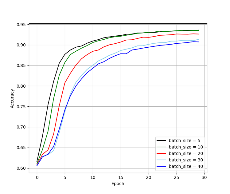
training data in terms of number
of batch size.

Fig. .13 shows the localization accuracy during the training in terms of different time steps, the overall performance increases with increasing time steps, but tradeoff is made considering practical situation and the increase in calculation burden. Accuracy of around 0.94 is reached with time step of 30 while a small time step as 10 could only reach accuracy of around 0.90.
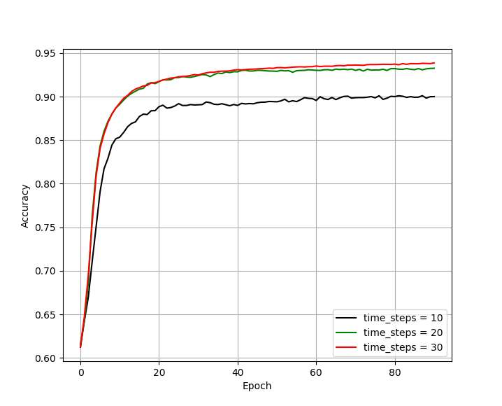
Table III shows the configuration of the final LSTM model optimized based on the training data and relevant parameters we set.
| LSTM Parameter | Value |
|---|---|
| Ratio of Training Data to Overall Data | 0.75 |
| Number of Epochs | 100 |
| Batch Size | 5 |
| Time Steps | 30 |
| Hidden Nodes | 128 |
| Optimizer | ADAM [15] |
| Loss | Mean Squared Error (MSE) |
| Dropout Rate | 0.2 |
V Discussions
V-A XJTLUIndoorLoc Database
Fig. 14 illustrates the frequency of each RSS measurement tested by Huawei smartphones on the two floors at IBSS building. Also, other databases have problems with APs being lost in either training or test data set due to a large timed gap between the two measurements for data sets, which is not the case for XJTLUIndoorLoc with as minimum of time as possible between the training and testing data measurements. Taking into account all these factors, XJTLUIndoorLoc enables accurate indoor localization despite the size of the area, different path directions, type of smart phone and the numbers and locations of buildings/floors.
However, there are also a few issues with the database:
- •
Difference in geomagnetic field values: The values obtained by the two smart phones were quite different from each other, though these values should be similar to each other.
- •
Deviation in manual measurement: The location of the smart phones may not match the reference points perfectly due to the varying heights of the users.
- •
The trained data used is one directional data: Theoretically, the rotational coordinates are best obtained by using rotation matrix or orientation.
- •
Inconsistency in using mobile devices: The MIX2 was only used on the 4th floor while the HUAWEI was used on both the 4th and 5th floors.
- •
Inconsistency with RSS Measurements: The numbers of RSS measurements with the two smart phones used on the 4th floor are different as shown in Fig. 14.


V-B CNN-Based Indoor Localization with RSS
The results of the CNN-based indoor localization was worse than the state-of-the-art DNN-based indoor localization. Fig. 15 shows the CNN results. There are possible explanations that should be discussed. Our database still need to be optimized because a major part of RSS stored in our database is inconsistent. The data fluctuates rapidly so the converted input images were different even for the same reference point. This prevents the network from learning efficiently. Moreover, the computational complexity is therefore raised to an extent where optimizing the algorithm will not grant improvement on the accuracy.
If the problem of the database can be solved, there are some proposed method for the optimization of CNN. As is mentioned in methodology section, the addition of dropout layer is effective. Similarly, the batch normalization layer can be added to reduce the computational complexity for max-pooling layer. As a result, the overall accuracy can be improved. Furthermore, adjusting relevant parameters (for instance weight decay, learning rate, etc.) can increase the performance of CNN. Then, if the input image are translated, zoomed proportionally or rotated and the network is trained with such data, the data augmentation will lead to better results.

V-C LSTM-Based Indoor Localization with Geomagnetic Field
In this work, the traces are created by the RWP. The speed and the direction will influence the result of the RWP model. In order to mimic the human trajectory indoor, the model needs to maximize the randomness. The result of the traditional RWP model has the speed damping. An intuitive display is the position of acute angle in trajectory. As shown in Fig. 7, the corners with black circles near the edge are sharper than the center corners, which is the probability of large events. The reason is that the time cost by the central points is more than edge points. This phenomenon causes the central tendency of the trace. To solve the problem, an improvement of the RWP model, which changed the node speed to satisfy the Gamma distribution, after changing the speed decay can be overcome [16]. In Gamma RWP, a random uniform distribution provides the initial position and direction of motion for each node [16]. Due to time constraints, this model can be used in the future to improve the personification of the trajectory, which may be helpful for training accuracy.
Fig. 16 shows the localization performance of the LSTM model with varying hidden nodes from 128 to 512. The middle blue box for each element in the figure represent the distribution of 75% total dataset, while the top and bottom line represent the distribution of 95% of dataset. We can conclude that with increasing hidden nodes, the general performance of the model would increase, but due to the phenomenon of overfitting, a few points (remaining 5% of hidden dataset) would deviate a lot from actual value. Although the mean error decrease from to when we increase the number of hidden nodes from 128 to 512, we observe that the maximum error increase from to . Moreover, for the performance of 128 hidden nodes, mean of 75% dataset is . Due to this overfitting problem, we choose the hidden nodes of 128 for a better overall performance.

VI Summary
We have presented a new fingerprinting database called XJTLUIndoorLoc for indoor localization and trajectory estimation based on Wi-Fi RSS and geomagnetic field. XJTLUIndoorLoc, which covers a 216- lobby and a 90- corridor, contains 969 reference points. For geomagnetic based localization, to improve the resolution of geomagnetic field map, Clough-Tocher 2-D interpolation was applied to the samples for the lobby, which increases the number of reference points from 663 to 21973. Then, we used RWP model to model the traces which served as training data for LSTM. The training result showed that the localization accuracy is highly aligned with the number of batch size, the number of hidden nodes as well as the number of time steps. Under optimum condition, the localization error over 25,000 samples reach a mean value of . We also described a new localization approach based on CNN with image-mapped RSS data; the current results indicate that there are lots of areas to improve. In the future, we plan to combine RSS and geomagnetic field to extend our work in this paper to improve the performance of indoor localization.
Acknowledgment
This work was supported in part by Xi’an Jiaotong-Liverpool University (XJTLU) Summer Undergraduate Research Fellowships programme (under Grant SURF-201830), Research Development Fund (under Grant RDF-16-02-39), Research Institute for Future Cities Research Leap Grant Programme 2016-2017 (under Grant RIFC2018-3), and Centre for Smart Grid and Information Convergence. The floor maps of the IBSS building were provided by XJTLU Campus Management Office.
References
- [1] J. Torres-Sospedra et al., “UJIIndoorLoc: A new multi-building and multi-floor database for WLAN fingerprint-based indoor localization problems,” in Proc. IPIN 2014, Busan, Korea, Oct. 2014, pp. 261–270.
- [2] J. Torres-Sospedra et al., “UjiIndoorLoc-Mag: A new database for magnetic field-based localization problems,” in Proc. IPIN 2015, Banff, Alberta, Canada, 2015, pp. 1–10.
- [3] P. Barsocchi et al., “A multisource and multivariate dataset for indoor localization methods based on WLAN and geo-magnetic field fingerprinting,” in Proc. IPIN 2016, Oct. 2016, pp. 1–8.
- [4] R. E. Kalman, “A new approach to linear filtering and prediction problems,” Transactions of the ASME, Series D, Journal of Basic Engineering, vol. 82, no. 1, pp. 35–45, Mar. 1960.
- [5] P. Alfeld, “A trivariate Clough-Tocher scheme for tetrahedral data,” Computer Aided Geometric Design, vol. 1, no. 2, pp. 169–181, Nov. 1984.
- [6] P. Nayak and P. Sinha, “Analysis of random way point and random walk mobility model for reactive routing protocols for MANET using NetSim simulator,” in Proc. AIMS 2015, Dec. 2015, pp. 427–432.
- [7] R. Collobert and J. Weston, “A unified architecture for natural language processing: Deep neural networks with multitask learning,” in Proc. ICML’08. New York, NY, USA: ACM, 2008, pp. 160–167. [Online].
- [8] A. van den Oord, S. Dieleman, and B. Schrauwen, “Deep content-based music recommendation,” in Proc. NIPS’13 – Volume 2, 2013, pp. 2643–2651.
- [9] M. Ibrahim, M. Elnainay, and M. Torki, “CNN based indoor localization using RSS time-series,” in Proc. IEEE ISCC, Natal, Brazil, Jun. 2018.
- [10] G. Jekabsons, V. Kairish, and V. Zuravlyov, “An analysis of Wi-Fi based indoor positioning accuracy,” J. Riga Technical University, vol. 44, pp. 131–137, Jan. 2011.
- [11] X. Wang, Z. Yu, and S. Mao, “DeepML: Deep LSTM for indoor localization with smartphone magnetic and light sensors,” in Proc. ICC 2018, May 2018, pp. 1–6.
- [12] H. J. Jang, J. M. Shin, and L. Choi, “Geomagnetic field based indoor localization using recurrent neural networks,” in Proc. GLOBECOM 2017, Dec. 2017, pp. 1–6.
- [13] J. Chung, Ç. Gülçehre, K. Cho, and Y. Bengio, “Empirical evaluation of gated recurrent neural networks on sequence modeling,” ArXiv e-prints, Dec. 2014. arXiv:1412.3555 [cs.NE].
- [14] K. Greff et al., “LSTM: A search space odyssey,” IEEE Trans. Neural Netw. Learn. Syst., vol. 28, no. 10, pp. 2222–2232, Oct. 2017.
- [15] D. Kingma and J. Ba, “ADAM: A method for stochastic optimization,” ArXiv e-prints, Jan. 2017.
- [16] N. Sabah and A. Hocanin, “An improved random waypoint mobility model for wireless ad-hoc network,” in Proc. ICIMT10 2010, 2010, pp. 146–150.