跳到论文正文
W Papers独立论文阅读器 arXiv:1810.07240 论文正文 计算阅读时间 · 0%
引用这篇论文根据当前论文元数据生成,正式投稿前建议核对。


License: arXiv.org perpetual non-exclusive license
arXiv:1810.07240v2 [stat.ME] 28 Nov 2018

Statistical classification for partially observed functional data via filtering

\AppendGraphicsExtensions

.tiff

Majid Mojirsheibani11 1 Corresponding author.  Email: majid.mojirsheibani@csun.edu This work is supported by the NSF Grant DMS-1407400 of Majid Mojirsheibani., My-Nhi Nguyen22 2 Email: mynhi.nguyen.324@my.csun.edu, and Crystal Shaw33 3 Email: c.shaw@ucla.edu

Department of Mathematics, California State University Northridge, CA, 91330, USA1,2

Department of Biostatistics, University of California Los Angeles, CA, 90095, USA3

Keywords: Classification, kernel, functional covariates, incomplete data.

Abstract

This article deals with the problem of functional classification for L2L^{2}-valued random covariates when some of the covariates may have missing or unobservable fragments. Here, it is allowed for both the training sample as well as the new unclassified observation to have missing fragments in their functional covariates. Furthermore, unlike most previous results in the literature, where covariate fragments are typically assumed to be missing completely at random, we do not impose any such assumptions here. Given the observed segments of the curves, we construct a kernel-type classifier which is quite straightforward to implement in practice. The proposed classifier is constructed based on dd-dimensional covariate vectors, obtained from the original covariate curves (by moving from L2L^{2} to the space ℓ2\ell_{2}), where dd itself is a parameter that has to be estimated. To estimate various parameters, we employ a random data-splitting approach which is easy to implement. We also establish the strong consistency of the proposed classifier and provide some numerical examples to assess its performance in finite sample problems.

1 Introduction

The problem of statistical classification and pattern recognition with functional covariates has received considerable attention in recent years. This is particularly true when the data are fully observable. In a standard two-group classification problem, this amounts to considering the random pair (𝝌,Y)(\boldsymbol{\chi},Y), where 𝝌\boldsymbol{\chi} is a functional covariate taking values in some metric space (ℳ,d)({\cal M},d) and Y∈{0,1}Y\in\{0,1\}, called the class membership or class variable, has to be predicted based on 𝝌\boldsymbol{\chi}. Here, one would like to find a classifier (a function) g:ℳ→{0,1}g:{\cal M}\to\{0,1\} for which the misclassification error, L(g):=P{g(𝝌)≠Y}L(g):=P\{g(\boldsymbol{\chi})\neq Y\}, is as small as possible. The optimal classifier, i.e., the classifier with the lowest misclassification error, is given by gB​(χ)=1g_{\mbox{\tiny B}}(\chi)=1 if P⁡{Y=1|𝝌=χ}>1/2P\{Y=1|\boldsymbol{\chi}=\chi\}>1/2, and gB​(χ)=0g_{\mbox{\tiny B}}(\chi)=0 otherwise; see, for example, Cérou and Guyader (2006), Abraham et al. (2006), as well as the monograph by Devroye, et al. (1996; Ch. 2). Although we have presented our setup for the popular binary case where Y∈{0,1}Y\in\{0,1\}, our discussions and results in this paper can be generalized in a straightforward manner to the multi-group classification problem where Y∈{1,2,…,C},Y\in\{1,2,\dots,C\}, for some positive integer C≥2C\geq 2.

In practice the optimal classifier gBg_{\mbox{\tiny B}} is virtually always unknown (because the conditional probability ℙ​{Y=1|𝝌=χ}\mathbb{P}\{Y=1|\boldsymbol{\chi}=\chi\} is not available) and one only has access to a set of nn independent and identically distributed (iid) data values 𝔻n={(𝝌1,Y1),…,(𝝌n,Yn)}\mathbb{D}_{n}=\{(\boldsymbol{\chi}_{1},Y_{1}),\dots,(\boldsymbol{\chi}_{n},Y_{n})\} from the underlying distribution of (𝝌,Y)(\boldsymbol{\chi},Y). The task of classification is then to use the data 𝔻n\mathbb{D}_{n} to construct a classification rule gng_{n} that can predict the class membership, YY, of a new curve 𝝌\boldsymbol{\chi} with low error rates. A variety of techniques have been proposed for the classification of functional data in the literature. One may divide these techniques into roughly two types: (a) those approaches that use the whole curve 𝝌\boldsymbol{\chi} to predict YY and (b) those that use the filtered curves to carry out classification; here, a filtered curve is a representation of a curve in the form of a vector. Relevant results corresponding to the approach used under (a) include the nonparametric functional approach of Ferraty and Vieu (2003), the nearest neighbor method used by Cérou and Guyader (2006), the kernel classifier of Abraham et al. (2006), the depth-based classifier of López-Pintado and Romo (2006), the robust functional classification of Cuevas et al. (2007), the wavelet approach of Chang et al. (2014), the robust functional classification of Alonso et al.(2014), and the work of Meister (2016) on the optimality properties of kernel regression and classification with functional covariates taking values in a general complete separable metric space.

On the other hand, relevant work under (b) includes the discrimination method of Hall et al. (2001), the functional classification method of Biau et al. (2005), the results of Leng and Müller (2006) on the classification of gene expression data as well as that of Song et al. (2008), the wavelet approach of Berlinet, et al. (2008), the componentwise classification approach of Delaigle, et al. (2012), the classification method in Delaigle and Hall (2012), the depth-depth plot approach of Mosler and Mozharovskyi (2017), and the functional classification method of Dai and Müller (2017). Some other relevant results (but in the context of functional regression) include the work of Cai and Hall (2006) on prediction in functional linear regression, the results of Hall and Horowitz (2007) on the estimation of a slope function in functional linear regression, and those of Yao and Müller (2010) on functional quadratic regression.

In this paper we employ methods that primarily fall under (b) above. More specifically, assuming that the functional covariates take values in a separable Hilbert space (and using the fact that such spaces are isomorphic to the space ℓ2\ell_{2}), the functional covariates will be replaced by dd-dim vectors where d≡d⁡(n)d\equiv d(n) is to be determined by the data; here, d⁡(n)→∞d(n)\to\infty, as n→∞n\to\infty. For the missing data framework, we follow the setup proposed by Bugni (2012), which has also been employed by Kraus (2015) as well as Mojirsheibani and Shaw (2018); this is described in Sections 2.1. In section 2.2 we propose a kernel classifier, under multiple missing patterns, and study its asymptotic properties. Some numerical examples are also given; these appear in Section 2.3. All proofs are deferred to Section 3.

2 Partially observed curves and the setup

2.1 Background

In standard functional classification, one typically assumes that each observation (covariate) 𝝌⁡(t)\boldsymbol{\chi}(t) is a smooth curve on some compact domain ℐ⊂ℝ\mathcal{I}\subset\mathbb{R}. Furthermore, the great majority of existing results assume that 𝝌⁡(t)\boldsymbol{\chi}(t) as well as 𝝌i​(t)\boldsymbol{\chi}_{i}(t), i=1,…,ni=1,\dots,n, do not have any missing or unobservable fragments over the domain ℐ\mathcal{I}. In contrast, here we allow 𝝌\boldsymbol{\chi} to be possibly missing (unobservable) on some subset(s) of its domain, i.e., the situation where one may only be able to observe certain segments of the full curve 𝝌\boldsymbol{\chi}. In fact, to the best of our knowledge, the problem of functional classification with partially observed covariates has received very little attention in the literature. Some key results along these lines in the literature appear to include the work of Delaigle and Hall (2013) who consider a quadratic discriminant classifier for censored functional data based on the observed fragments of covariates with overlapping domains that are not too short. Another relevant result here is that of Kraus (2015) who proposes methods to estimate parameters and to carry out principal component analysis with missing data. These authors assume that the missingness is independent of the covariate and response variables, which amounts to having covariates missing completely at random (MCAR). In this paper we do not impose any MCAR assumptions. More specifically, let (Ω,𝒜,ℙ)(\Omega,{\cal A},\mathbb{P}) be the underlying probability space and let ℳ\mathcal{M} be the space of square-integrable functions L2​(ℐ)L^{2}(\mathcal{I}), where ℐ{\cal I} is an interval on the real line. Therefore, 𝝌\boldsymbol{\chi} is a random function on (Ω,𝒜,ℙ)(\Omega,{\cal A},\mathbb{P}) with values (i.e., with sample paths) in L2​(ℐ)L^{2}({\cal I}). But, instead of observing the full curve 𝝌:Ω→L2​(ℐ)\boldsymbol{\chi}:\Omega\to L^{2}({\cal I}), one might only be able to observe certain segments of the curve denoted by 𝝌|s\boldsymbol{\chi}|_{s}, i.e., the restriction of the curve 𝝌⁡(t)\boldsymbol{\chi}(t) to t∈s⊂ℐt\in s\subset\mathcal{I}.

To set up our framework for possible missing patterns in the curve 𝝌\boldsymbol{\chi}, we follow the setup proposed by Bugni (2012). This method is also employed by Kraus (2015) who considers principal component analysis with missing data. In Bugni’s (2012) setup, it is assumed that for a fine enough partition of ℐ{\cal I} into J<∞J<\infty subintervals ℐ1,…,ℐJ{\cal I}_{1},\dots,{\cal I}_{J}, each sample function of 𝝌\boldsymbol{\chi} is either completely observed or completely unobserved within each of these JJ subintervals. Some examples of such functional variables can be found in Bugni (2012). In the rest of this paper we assume that there are M<2JM<2^{J} possible missing patterns in the data where MM is usually much smaller than 2J2^{J}. Therefore, under the kk-th pattern, one observes the fragment 𝝌|sk\boldsymbol{\chi}|_{s_{k}}, k=1,…,Mk=1,\dots,M. Next, let δ\delta be the {1,…,M}\{1,\dots,M\}-valued random variable defined as

δ=kif pattern k (i.e., the fragment 𝝌|sk) is observed,k=1,…,M.\delta=k~~~\mbox{if pattern $k$ (i.e., the fragment $\boldsymbol{\chi}|_{s_{k}}$) is observed},~k=1,\dots,M.

Therefore, if we let 𝝌(δ)\boldsymbol{\chi}^{(\delta)} represent the observed covariate fragment, then it can be written as 𝝌(δ)=∑k=1M𝝌|skI{δ=k}\boldsymbol{\chi}^{(\delta)}=\sum_{k=1}^{M}\boldsymbol{\chi}|_{s_{k}}\,I\{\delta=k\}, where, without loss of generality, one may take s1=ℐs_{1}=\mathcal{I}, i.e., the case where the entire curve 𝝌\boldsymbol{\chi} is observable on ℐ\mathcal{I}. In passing we also note that when pattern kk is observed, then a classifier is any function of the form  gk:L2​(sk)→{0,1}g_{k}:L^{2}(s_{k})\to\{0,1\}. Therefore, given MM possible missing patterns, any classifier is necessarily of the form

Γ0(𝝌(δ))=∑k=1MI{δ=k}⋅gk(𝝌|sk),for some gk:L2(sk)→{0,1},k=1,…,M.\Gamma_{0}(\boldsymbol{\chi}^{(\delta)})=\sum_{k=1}^{M}I\{\delta=k\}\cdot g_{k}(\boldsymbol{\chi}|_{s_{k}}),~~\mbox{for some $g_{k}:L^{2}(s_{k})\to\{0,1\},~k=1,\dots,M$.} (1)

As for the theoretically best classifier for the current setup (with missing fragments in 𝝌\boldsymbol{\chi}), let ϕk(χ|sk)=E[(2Y−1)I{δ=k}|𝝌(t)=χ(t),t∈sk]\phi_{k}(\chi|_{s_{k}})=E\left[(2Y-1)I\{\delta=k\}\,\big|\,\boldsymbol{\chi}(t)=\chi(t),~t\in s_{k}\right] and consider the classifier

Γ0B(𝝌(δ))=∑k=1MI{δ=k}⋅I{ϕk(𝝌|sk)>0}.\Gamma_{0}^{\mbox{\tiny B}}(\boldsymbol{\chi}^{(\delta)})=\sum_{k=1}^{M}I\{\delta=k\}\cdot I\{\phi_{k}(\boldsymbol{\chi}|_{s_{k}})>0\}. (2)

The following result shows that Γ0B\Gamma_{0}^{\mbox{\tiny B}} is the optimal classifier (it has the lowest error).

Theorem 1

[Mojirsheibani and Shaw (2018; Theorem 1).]
The classifier Γ0B\Gamma_{0}^{\mbox{\tiny B}} defined by (2) is optimal in the sense that for any other classifier Γ0\Gamma_{0}, one has ℙ{Γ0B(𝛘(δ))≠Y}≤ℙ{Γ0(𝛘(δ))≠Y}\mathbb{P}\{\Gamma_{0}^{\mbox{\tiny B}}(\boldsymbol{\chi}^{(\delta)})\neq Y\}\leq\mathbb{P}\{\Gamma_{0}(\boldsymbol{\chi}^{(\delta)})\neq Y\}.

We note that since any classifier Γ\Gamma is of the form (1), Theorem 1 implies that

ℙ{Γ0B(𝝌(δ))≠Y}=infgk:L2(sk)→{0,1},k=1,…,Mℙ{∑k=1MI{δ=k}⋅gk(𝝌|sk)≠Y}.\displaystyle\mathbb{P}\left\{\Gamma_{0}^{\mbox{\tiny B}}(\boldsymbol{\chi}^{(\delta)})\neq Y\right\}=\inf_{g_{k}:~L^{2}(s_{k})\to\{0,1\},~k=1,\dots,M~}\,\mathbb{P}\left\{\mbox{$\sum_{k=1}^{M}$}I\{\delta=k\}\cdot g_{k}(\boldsymbol{\chi}|_{s_{k}})\neq Y\right\}.

Since 𝝌∈L2​(ℐ)\boldsymbol{\chi}\in L^{2}(\mathcal{I}), which is a separable Hilbert space, it can be expressed by the expansion 𝝌⁡(t)=∑j=1∞Xj​ψj​(t)\boldsymbol{\chi}(t)=\sum_{j=1}^{\infty}X_{j}\psi_{j}(t), where {ψ1,ψ2,…}\{\psi_{1},\psi_{2},...\} is a complete orthonormal basis for L2​(ℐ)L^{2}(\mathcal{I}) and Xj=⟨𝝌,ψj⟩:=∫ℐ𝝌⁡(t)​ψj​(t)​𝑑tX_{j}=\langle\boldsymbol{\chi},\psi_{j}\rangle:=\int_{\mathcal{I}}\boldsymbol{\chi}(t)\psi_{j}(t)dt. Here the infinite sum converges in L2L^{2}. Similarly, given the data (𝝌i,Yi),i=1,…,n(\boldsymbol{\chi}_{i},Y_{i}),~i=1,...,n, we can write 𝝌i​(t)=∑j=1∞Xi​j​ψj​(t)\boldsymbol{\chi}_{i}(t)=\sum_{j=1}^{\infty}X_{ij}\psi_{j}(t), with Xi​j=∫ℐ𝝌i​(t)​ψj​(t)​𝑑tX_{ij}=\int_{\mathcal{I}}\boldsymbol{\chi}_{i}(t)\psi_{j}(t)dt. Since any infinite-dimensional separable Hilbert space is isomorphic to the space ℓ2={𝐱=(x1,x2,…)|∑i=1∞|xi|2<∞}\ell_{2}=\big\{{\bf x}=(x_{1},x_{2},\dots)\big|\sum_{i=1}^{\infty}|x_{i}|^{2}<\infty\big\}, the scores Xi​j,j≥1X_{ij},~j\geq 1, are used as surrogates for the datum 𝝌i\boldsymbol{\chi}_{i} in the literature in the sense that knowing 𝕏i:=(Xi​1,Xi​2,…)\mathbb{X}_{i}:=(X_{i1},X_{i2},\dots) is the same as knowing 𝝌i\boldsymbol{\chi}_{i}; see, for example, Hall et al (2001) or Biau et al (2005). This fact is also formalized in part (ii) of Theorem 2 of the current paper for the particular case of classification with missing functional covariates.

To simplify our presentation, we first look at the oversimplified case where there is only one missing pattern. More specifically, write ℐ=[a,b]=[a,c]∪(c,b]\mathcal{I}=[a,b]=[a,c]\cup(c,b], for some a<c<ba<c<b, where 𝝌⁡(t)\boldsymbol{\chi}(t) may be missing on (c,b](c,b] only. Therefore, we have the expansions

𝝌⁡(t)\displaystyle{\boldsymbol{\chi}(t)} =\displaystyle= ∑j=1∞⟨𝝌,ψj⟩[a,b]​ψj​(t)=∑j=1∞[∫ac𝝌⁡(t)​ψj​(t)​𝑑t+∫cb𝝌⁡(t)​ψj​(t)​𝑑t]​ψj​(t)\displaystyle\sum_{j=1}^{\infty}\left\langle\boldsymbol{\chi},\psi_{j}\right\rangle_{[a,b]}\psi_{j}(t)\,=\,\sum_{j=1}^{\infty}\left[\int_{a}^{c}\boldsymbol{\chi}(t)\psi_{j}(t)dt+\int_{c}^{b}\boldsymbol{\chi}(t)\psi_{j}(t)dt\right]\psi_{j}(t)
=\displaystyle= ∑j=1∞(⟨𝝌,ψj⟩[a,c]+⟨𝝌,ψj⟩[c,b])​ψj​(t).\displaystyle\sum_{j=1}^{\infty}\big(\left\langle\boldsymbol{\chi},\psi_{j}\right\rangle_{[a,c]}+\left\langle\boldsymbol{\chi},\psi_{j}\right\rangle_{[c,b]}\big)\,\psi_{j}(t).

Now the surrogate vector of score functions can be written as

𝐗\displaystyle{\bf X} =\displaystyle= (X1,X2,…):=(⟨𝝌,ψ1⟩[a,b],⟨𝝌,ψ2⟩[a,b],…)\displaystyle(X_{1},X_{2},\dots):=\big(\langle\boldsymbol{\chi},\psi_{1}\rangle_{\mbox{\tiny$[a,b]$}}\,,\,\langle\boldsymbol{\chi},\psi_{2}\rangle_{\mbox{\tiny$[a,b]$}}\,,\dots\big)
=\displaystyle= (⟨𝝌,ψ1⟩[a,c],⟨𝝌,ψ2⟩[a,c],…)+(⟨𝝌,ψ1⟩[c,b],⟨𝝌,ψ2⟩[c,b],…)\displaystyle\big(\langle\boldsymbol{\chi},\psi_{1}\rangle_{\mbox{\tiny$[a,c]$}}\,,\,\langle\boldsymbol{\chi},\psi_{2}\rangle_{\mbox{\tiny$[a,c]$}}\,,\dots\big)+\big(\langle\boldsymbol{\chi},\psi_{1}\rangle_{\mbox{\tiny$[c,b]$}}\,,\,\langle\boldsymbol{\chi},\psi_{2}\rangle_{\mbox{\tiny$[c,b]$}}\,,\dots\big)
=:\displaystyle=: (Z1,Z2,…)+(V1,V2,…)\displaystyle(Z_{1},Z_{2},\dots)+(V_{1},V_{2},\dots)
=:\displaystyle=: 𝐙+𝐕,\displaystyle{\bf Z}+{\bf V},

where V may be missing, but not Z. Here, we note that if V is not missing then 𝐗=Z+V{\bf X}=\textbf{Z}+\textbf{V} is fully observable, otherwise the classification will be based on Z only. In fact, if we put

ϕ1(𝐗)=𝔼[(2Y−1)I{δ=1}|𝐗]andϕ0(𝐙)=𝔼[(2Y−1)I{δ=2}|𝐙],\phi_{1}({\bf X})=\mathbb{E}\left[(2Y-1)I\{\delta=1\}\big|{\bf X}\right]~~\mbox{and}~~\phi_{0}({\bf Z})=\mathbb{E}\left[(2Y-1)I\{\delta=2\}\big|{\bf Z}\right],

where δ=1\delta=1 if 𝐗{\bf X} is fully observable (otherwise δ=2\delta=2), and define the classifier

ΓB(𝐗(δ))=I{δ=1}I{ϕ1(𝐗)>0}+I{δ=2}I{ϕ0(𝐙)>0},\Gamma^{\mbox{\tiny B}}({\bf X}^{(\delta)})=I\{\delta=1\}I\big\{\phi_{1}({\bf X})>0\big\}+I\{\delta=2\}I\big\{\phi_{0}({\bf Z})>0\big\},

where 𝐗(δ)=I{δ=1}𝐗+I{δ=2}𝐙{\bf X}^{(\delta)}=I\big\{\delta=1\big\}{\bf X}+I\big\{\delta=2\big\}{\bf Z} represents the observable covariate, then it follows from our Theorem 2 below that the classifier ΓB\Gamma^{\mbox{\tiny B}} has the lowest misclassification error. In the more general setting with M missing patterns, if we let Xj(k)=⟨𝝌,ψj⟩skX_{j}^{(k)}=\langle{\boldsymbol{\chi}},\psi_{j}\rangle_{s_{k}} then, with s1:=ℐs_{1}:=\mathcal{I}, we have the vectors of scores

𝐗(k)=(X1(k),X2(k),…)=(⟨𝝌,ψ1⟩sk,⟨𝝌,ψ2⟩sk,……),k=1,…,M.{\bf X}^{(k)}=(X_{1}^{(k)},X_{2}^{(k)},\dots)=\big(\langle{\boldsymbol{\chi}},\psi_{1}\rangle_{s_{k}},\langle{\boldsymbol{\chi}},\psi_{2}\rangle_{s_{k}},\dots\dots\big),~k=1,\dots,M.

Clearly, when δ=k\delta=k, we only observe 𝐗(k){\bf X}^{(k)} in which case a classifier is any function of the form gk:ℓ2→{0,1}.g_{k}:\ell_{2}\to\{0,1\}. Hence, any classifier can be written in the general form

Γ(𝐗(δ))=∑k=1MI{δ=k}⋅gk(𝐗(k)),where𝐗(δ):=∑k=1M𝐗(k)I{δ=k}.\displaystyle\Gamma({\bf X}^{(\delta)})=\sum_{k=1}^{M}I\{\delta=k\}\cdot g_{k}({\bf X}^{(k)}),~~\mbox{where}~~{\bf X}^{(\delta)}:=\sum_{k=1}^{M}{\bf X}^{(k)}I\{\delta=k\}. (3)

Now, let

ϕk(𝐗(k))=E[(2Y−1)I{δ=k}|𝐗(k)],k=1,…,M,\phi_{k}({\bf X}^{(k)})=E\left[(2Y-1)I\{\delta=k\}\,\big|\,{\bf X}^{(k)}\right],~k=1,\dots,M, (4)

and define the following classifier (which can be viewed as the counterpart of (2) on ℓ2\ell_{2})

ΓB(𝐗(δ))=∑k=1MI{δ=k}⋅I{ϕk(𝐗k)>0}.\Gamma^{\mbox{\tiny B}}({\bf X}^{(\delta)})=\sum_{k=1}^{M}I\{\delta=k\}\cdot I\{\phi_{k}({\bf X}^{k})>0\}. (5)

Then part (i) of the following result shows that the classifier in (5) is optimal.

Theorem 2

Let ΓB\Gamma^{\mbox{\tiny B}} be the classifier given by (5). Then

(i) The classifier ΓB\Gamma^{\mbox{\tiny B}} has the lowest misclassification error, i.e., for any other classifier Γ\Gamma, one has ℙ{ΓB(𝐗(δ))≠Y}≤ℙ{Γ(𝐗(δ))≠Y}\mathbb{P}\{\Gamma^{\mbox{\tiny B}}({\bf X}^{(\delta)})\neq Y\}\leq\mathbb{P}\{\Gamma({\bf X}^{(\delta)})\neq Y\}.

(ii) The misclassification error of the optimal classifier based on the whole curve is the same as that of the optimal classifier based on the filtered curve, i.e., ℙ{Γ0B(𝛘(δ))≠Y}=ℙ{ΓB(𝐗(δ))≠Y}\mathbb{P}\{\Gamma_{0}^{\mbox{\tiny B}}(\boldsymbol{\chi}^{(\delta)})\neq Y\}=\mathbb{P}\{\Gamma^{\mbox{\tiny B}}({\bf X}^{(\delta)})\neq Y\}, where ΓB​(𝐗(δ))\Gamma^{\mbox{\tiny B}}({\bf X}^{(\delta)}) and Γ0B​(𝛘(δ))\Gamma_{0}^{\mbox{\tiny B}}(\boldsymbol{\chi}^{(\delta)}) are as in (5) and (2), respectively.

(iii) Let Γ\Gamma be any classifier of the form Γ(𝐗(δ))=∑k=1MI{δ=k}⋅I{φk(𝐗(k))>0}\Gamma({\bf X}^{(\delta)})=\sum_{k=1}^{M}I\{\delta=k\}\cdot I\{\varphi_{k}({\bf X}^{(k)})>0\} for some functions φk:ℓ2→[−1,1],k=1,…,M.\varphi_{k}:\ell_{2}\to[-1,1],~k=1,\dots,M. Then ℙ{Γ(𝐗(δ))≠Y}−ℙ{ΓB(𝐗(δ))≠Y}≤∑k=1M𝔼|ϕk(𝐗(k))−φk(𝐗(k))|\mathbb{P}\big\{\Gamma({\bf X}^{(\delta)})\neq Y\big\}-\mathbb{P}\big\{\Gamma^{\mbox{\tiny B}}({\bf X}^{(\delta)})\neq Y\big\}\leq\sum_{k=1}^{M}\mathbb{E}\big|\phi_{k}({\bf X}^{(k)})-\varphi_{k}({\bf X}^{(k)})\big|, where ϕk​(𝐗(k))\phi_{k}({\bf X}^{(k)}) is as in (4).

Remark 1

Part (iii) of Theorem 2 provides a useful tool to bound the difference between the two misclassification errors in terms of the difference between ϕk​(𝐗(k))\phi_{k}({\bf X}^{(k)}) that appears in (4) and the function φk​(𝐗(k))\varphi_{k}({\bf X}^{(k)}). Here, one can think of φk​(𝐗(k))\varphi_{k}({\bf X}^{(k)}) as an approximation to the unknown function ϕk(𝐗(k))=𝔼[(2Y−1)I{δ=k}|𝐗(k)]\phi_{k}({\bf X}^{(k)})=\mathbb{E}\left[(2Y-1)I\{\delta=k\}\,\big|\,{\bf X}^{(k)}\right]. Part (ii) of the theorem, which states that the error of the optimal classifier on L2L^{2} is the same as that of the optimal classifier in ℓ2\ell_{2}, is rather intuitive.

2.2 Reduction to finite dimensions and the proposed classifier

Since working in ℓ2\ell_{2} is not convenient from a practical point of view, in what follows we consider finite-dimensional versions of the classifier ΓB\Gamma^{\mbox{\tiny B}} defined in (5) where 𝐗(k){\bf X}^{(k)} will be replaced by the dd-dimensional vector 𝐗(d,k)=(X1(k),…,Xd(k))=(⟨𝝌,ψ1⟩sk,…,⟨𝝌,ψd⟩sk){\bf X}^{(d,k)}=(X_{1}^{(k)},\dots,X_{d}^{(k)})=(\langle\boldsymbol{\chi},\psi_{1}\rangle_{s_{k}},\dots,\langle\boldsymbol{\chi},\psi_{d}\rangle_{s_{k}}), k=1,…,Mk=1,\dots,M, (a data-driven choice of the parameter dd is discussed later in this section). More specifically, define the function ϕd,k:ℝd→[−1,1]\phi_{d,k}:\mathbb{R}^{d}\to[-1,1] by

ϕd,k(𝐗(d,k))=𝔼[(2Y−1)I{δ=k}|𝐗(d,k)]=E[(2Y−1)I{δ=k}|X1(k),…,Xd(k)],\phi_{d,k}({\bf X}^{(d,k)})=\mathbb{E}\left[(2Y-1)I\{\delta=k\}\,\big|\,{\bf X}^{(d,k)}\right]=E\left[(2Y-1)I\{\delta=k\}\,\big|\,X_{1}^{(k)},\dots,X_{d}^{(k)}\right], (6)

k=1,…,M,k=1,\dots,M, and consider the following version of the classifier in (5)

ΓB,d(𝐗(d,δ))=∑k=1MI{δ=k}⋅I{ϕd,k(𝐗(d,k))>0}.\Gamma^{\mbox{\tiny B},d}({\bf X}^{(d,\delta)})=\sum_{k=1}^{M}I\{\delta=k\}\cdot I\left\{\phi_{d,k}({\bf X}^{(d,k)})>0\right\}. (7)

Here, 𝐗(d,δ)=∑k=1M𝐗(d,k)⋅I{δ=k}{\bf X}^{(d,\delta)}=\sum_{k=1}^{M}{\bf X}^{(d,k)}\cdot I\{\delta=k\}. The following result shows that the classifier ΓB,d\Gamma^{\mbox{\tiny B},d} is optimal:

Theorem 3

Let ΓB,d\Gamma^{\mbox{\tiny B},d} be the classifier in (7). Then for any other classifier Γ\Gamma we have ℙ{ΓB,d(𝐗(d,δ))\mathbb{P}\{\Gamma^{\mbox{\tiny B},d}({\bf X}^{(d,\delta)}) ≠Y}≤ℙ{Γ(𝐗(d,δ))≠Y}.\neq Y\}\leq\mathbb{P}\{\Gamma({\bf X}^{(d,\delta)})\neq Y\}.

The fact that all distributions are unknown implies that the classifier in (7) is not available in practice and has to be constructed based on the available data. Here we propose a kernel-type methodology. To construct our kernel classifier, we also employ the following data-splitting approach which is in the spirit of the method proposed by Biau et al (2005) in the case of functional nearest neighbor classification (without any missing data). Let 𝐗(δ){\bf X}^{(\delta)} be as in (3) and start by randomly splitting the data 𝔻n={(𝐗1(δ1),Y1,δ1),…,(𝐗n(δn),\mathbb{D}_{n}=\{({\bf X}_{1}^{(\delta_{1})},Y_{1},\delta_{1}),\dots,({\bf X}_{n}^{(\delta_{n})}, Yn,δn)}Y_{n},\delta_{n})\} into a training sample 𝔻m\mathbb{D}_{m} of size mm and a testing sequence 𝔻ℓ\mathbb{D}_{\ell} of size ℓ=n−m\ell=n-m. Here, mm and ℓ\ell typically depend on nn (they grow with nn). Next, put

ϕ^m,d,hk(𝐗(d,k))=∑i:(𝐗(δi),Yi,δi)∈𝔻m(2Yi−1)I{δi=k}𝒦k(𝐗(d,k)−𝐗i(d,k)hk),\widehat{\phi}_{m,d,\,h_{k}}({\bf X}^{(d,k)})=\sum_{i:~({\bf X}^{(\delta_{i})},Y_{i},\delta_{i})\in\mathbb{D}_{m}}(2Y_{i}-1)I\{\delta_{i}=k\}\mathcal{K}_{k}\left(\frac{{\bf X}^{(d,k)}-{\bf X}_{i}^{(d,k)}}{h_{k}}\right)\,,~~~~~ (8)

where 𝐗(d,k){\bf X}^{(d,k)} and 𝐗i(d,k){\bf X}_{i}^{(d,k)} represent the first dd components of 𝐗(k){\bf X}^{(k)} and 𝐗i(k){\bf X}_{i}^{(k)}, respectively, and where 𝒦k:ℝd→ℝ+\mathcal{K}_{k}:\mathbb{R}^{d}\to\mathbb{R}_{+} is the kernel used with the smoothing parameter hkh_{k}, and define the kernel-type classifier

Γmd(𝐗(d,δ))=∑k=1MI{δ=k}I{ϕ^m,d,hk(𝐗(d,k))>0}.\Gamma_{m}^{d}({\bf X}^{(d,\delta)})=\sum_{k=1}^{M}I\{\delta=k\}I\left\{\widehat{\phi}_{m,d,h_{k}}({\bf X}^{(d,k)})>0\right\}. (9)

Let, ℋ≡ℋn\mathcal{H}\equiv\mathcal{H}_{n} be a grid of positive values from which h1,…​hMh_{1},\dots h_{M} are to be selected, and define d^\widehat{d} and h^k\widehat{h}_{k} to be the empirically chosen values of dd and hkh_{k}, k=1,…,Mk=1,\dots,M, based on the testing sequence 𝔻ℓ\mathbb{D}_{\ell}, i.e.,

(d^,h^1,…,h^M)=argmin1≤d≤dn,hk∈ℋn,k=1,…,Mℓ−1∑i:(𝐗(δi),Yi,δi)∈𝔻ℓI{Ωi(m,d,h1,…,hM)},(\widehat{d},\widehat{h}_{1},\dots,\widehat{h}_{M})=\operatornamewithlimits{argmin}_{1\leq d\leq d_{n},\,h_{k}\in\mathcal{H}_{n},\,k=1,\dots,M~}\ell^{-1}\sum_{i:~{(\bf X}^{(\delta_{i})},Y_{i},\delta_{i})\in\mathbb{D}_{\ell}}I\big\{\Omega_{i}(m,d,h_{1},\dots,h_{M})\big\}, (10)

where the set Ωi\Omega_{i} is given by

Ωi(m,d,h1,…,hM)={∑k=1MI{δi=k}⋅I{ϕ^m,d,hk(𝐗i(d,k))>0}≠Yi},\Omega_{i}(m,d,h_{1},\dots,h_{M})=\left\{\sum_{k=1}^{M}I\{\delta_{i}=k\}\cdot I\left\{\widehat{\phi}_{m,d,h_{k}}({\bf X}_{i}^{(d,k)})>0\right\}\neq Y_{i}\right\}, (11)

and where dnd_{n} diverges with nn but not too rapidly (see Remark 2). The final classifier is then the plug-in version of (9) given by

Γ^n(𝐗(d^,δ))=∑k=1MI{δ=k}I{ϕ^n,d^,h^k(𝐗(d^,k))>0},\widehat{\Gamma}_{n}({\bf X}^{(\widehat{d},\delta)})=\sum_{k=1}^{M}I\{\delta=k\}I\left\{\widehat{\phi}_{n,\widehat{d},\widehat{h}_{k}}({\bf X}^{(\widehat{d},k)})>0\right\}, (12)

where the subscript nn used in (12) indicates that it is constructed based on the entire data of size nn. How good is the classifier Γ^n\widehat{\Gamma}_{n} in (12)? The next theorem shows that under rather minimal assumptions Γ^n\widehat{\Gamma}_{n} is strongly optimal, i.e., ℙ{Γ^n(𝐗(d^,δ))≠Y|𝔻n}→a.s.ℙ{ΓB(𝐗(δ))≠Y},\mathbb{P}\{\widehat{\Gamma}_{n}({\bf X}^{(\widehat{d},\delta)})\neq Y|\mathbb{D}_{n}\}\to^{\mbox{\small a.s.}}~\mathbb{P}\{\Gamma^{\mbox{\tiny B}}({\bf X}^{(\delta)})\neq Y\}, as n→∞n\to\infty. To present our main results, we first state the following assumption on the kernels used in (8).

Assumption (K).
The kernel 𝒦k\mathcal{K}_{k} used in (8) is regular: A nonnegative kernel 𝒦\mathcal{K} is said to be regular if there are positive constants b>0b>0 and r>0r>0 for which 𝒦(x)≥bI{x∈S0,r}\mathcal{K}(\textbf{x})\geq bI\{\textbf{x}\in S_{0,r}\} and ∫supy∈x+S0,r𝒦⁡(y)​𝑑x<∞,\int\sup_{\textbf{y}\in\textbf{x}+S_{0,r}}\mathcal{K}(\textbf{y})d\textbf{x}<\infty, where S0,rS_{0,r} is the ball of radius rr centered at the origin. (For more on regular kernels see, for example, Györfi et al (2002).)

Theorem 4

Suppose that Assumption (K) holds. Also assume that, as n→∞n\to\infty, we have ℓ≡ℓ⁡(n)→∞\ell\equiv\ell(n)\to\infty, m≡m⁡(n)→∞m\equiv m(n)\to\infty, ℓ−1​log⁡|ℋn|→0\ell^{-1}\log|\mathcal{H}_{n}|\to 0, and ℓ−1​log⁡dn→0\ell^{-1}\log d_{n}\to 0, where |ℋn||\mathcal{H}_{n}| is the cardinality of the set ℋn\mathcal{H}_{n}. Suppose that for each k=1,…,Mk=1,\dots,M, there is an hk≡hk​(n)∈ℋnh_{k}\equiv h_{k}(n)\in\mathcal{H}_{n} such that max1≤k≤M⁡hk→0\max_{1\leq k\leq M}h_{k}\to 0 and min1≤k≤M⁡m​hkdn→∞\min_{1\leq k\leq M}mh_{k}^{d_{n}}\to\infty, as n→∞n\to\infty. Then the classifier Γ^n\widehat{\Gamma}_{n} is asymptotically strongly optimal, i.e.,

ℙ{Γ^n(𝐗(d^,δ))≠Y|𝔻n}⟶a.s.ℙ{ΓB(𝐗(δ))≠Y},\mathbb{P}\left\{\widehat{\Gamma}_{n}({\bf X}^{(\widehat{d},\delta)})\neq Y\,\big|\,\mathbb{D}_{n}\right\}\longrightarrow^{\mbox{\rm\small a.s.}}~\mathbb{P}\left\{\Gamma^{\mbox{\tiny B}}({\bf X}^{(\delta)})\neq Y\right\},

as n→∞n\to\infty, where ΓB\Gamma^{\mbox{\tiny B}} is the theoretically optimal classifier appearing in Theorem 2.

Remark 2

The conditions imposed on hk≡hk​(n)h_{k}\equiv h_{k}(n) and dnd_{n} in the statement of Theorem 4 are satisfied if dnd_{n} does not grow too rapidly and hkh_{k} converges to zero slowly, as n→∞n\to\infty. In fact, if we take dn=(log⁡nc0)1−γd_{n}=(\log n^{c_{0}})^{1-\gamma} for any c0>0c_{0}>0 and any 0<γ<10<\gamma<1, and if, for example, hk=(log⁡nck)−1h_{k}=(\log n^{c_{k}})^{-1} for any ck>0c_{k}>0, then it is straightforward to see that m​hkdn→∞,mh_{k}^{d_{n}}\to\infty, as n→∞n\to\infty. Intuitively, the slow rate of convergence (logarithmic) of hkh_{k} to zero is not necessarily unrealistic here and, in a sense, can be tied to the increasing dimension dnd_{n}. In fact, in what Ferraty and Vieu (2006; page 211) refer to as the curse of infinite dimensionality, the authors argue that in the problem of kernel regression estimation for the general regression function 𝔼⁡[Y|𝐗=𝐱]\mathbb{E}[Y|{\bf X}={\bf x}] with a functional covariate 𝐗{\bf X}, the smoothing parameter h≡h⁡(n)h\equiv h(n) can be of order (log⁡n)u(\log n)^{u} for some u<0u<0.

2.3 Numerical examples

2.3.1 Simulated Data

Here, we provide some numerical examples to assess the performance of the methods proposed in the previous section. In this analysis, we develop classifiers to predict the unknown class Y=0Y=0 or Y=1Y=1 of a functional covariate 𝝌⁡(t)\boldsymbol{\chi}(t), defined in L2​([0,1])L^{2}([0,1]), that may have missing fragments. Adopting the missing pattern setup of Section 2.1, without loss of generality let s1:=ℐ=[0,1]s_{1}:=\mathcal{I}=[0,1]. Also, let s2=[0,0.3]∪[0.5,1]⊂ℐs_{2}=[0,0.3]\cup[0.5,1]\subset\mathcal{I}, s3=[0,0.1]∪[0.2,0.45]∪[0.6,0.85]∪[0.9,1]⊂ℐs_{3}=[0,0.1]\cup[0.2,0.45]\cup[0.6,0.85]\cup[0.9,1]\subset\mathcal{I}, s4=[0.25,0.5]∪[0.65,1]⊂ℐs_{4}=[0.25,0.5]\cup[0.65,1]\subset\mathcal{I}, and s5=[0,0.2]∪[0.3,0.55]∪[0.75,0.9]⊂ℐs_{5}=[0,0.2]\cup[0.3,0.55]\cup[0.75,0.9]\subset\mathcal{I}. We consider two cases of missing patterns: M=3M=3 and M=5M=5. In the case of M=3M=3, the patterns used are s1s_{1}, s2s_{2}, and s3s_{3}. Next, samples of functional observations (𝝌i(δi),Yi,δi),i=1,…,n\big(\boldsymbol{\chi}^{(\delta_{i})}_{i},Y_{i},\delta_{i}\big),~i=1,\dots,n, are generated based on rules which are similar to the approach of Rachdi and View (2007) and Mojirsheibani and Shaw (2018) as follows:

𝝌i(t)=Ai(t−0.5)2+Bi,i=1,2,…,n\boldsymbol{\chi}_{i}(t)=A_{i}(t-0.5)^{2}+B_{i},~~~\,i=1,2,\dots,n

where t∈s=s1,s2,s3,s4t\in s=s_{1},s_{2},s_{3},s_{4}, or s5s_{5} depending on whether δi=1,2,3,4\delta_{i}=1,2,3,4 or 55. Regarding the values of AiA_{i} and BiB_{i}, if Yi=1Y_{i}=1 then Ai​∼iid​N​(5,22)A_{i}\overset{\mbox{\tiny iid}}{\sim}N(5,2^{2}) and Bi​∼iid​N​(1,0.52)B_{i}\overset{\mbox{\tiny iid}}{\sim}N(1,0.5^{2}), otherwise if Yi=0Y_{i}=0 then Ai​∼iid​Unif​(0,5)A_{i}\overset{\mbox{\tiny iid}}{\sim}\mbox{Unif}\,(0,5) and Bi​∼iid​Unif​(0,1)B_{i}\overset{\mbox{\tiny iid}}{\sim}\mbox{Unif}\,(0,1). The class probabilities are taken to be P⁡(Y=1)=0.5=P⁡(Y=0)P(Y=1)=0.5=P(Y=0). With respect to the missing probability mechanism, we consider a logistic-type model

P{δ=1|Y=y,𝝌(t)=χ(t),t∈ℐ}=exp⁡{a⁡(1−y)+b​∫sχ⁡(t)​𝑑t+c​∫[0,1]∖st⋅χ⁡(t)​𝑑t}1+exp⁡{a⁡(1−y)+b​∫sχ⁡(t)​𝑑t+c​∫[0,1]∖st⋅χ⁡(t)​𝑑t},P\big\{\delta=1\,\big|Y=y,\mbox{$\boldsymbol{\chi}$}(t)=\chi(t),t\in\mathcal{I}\big\}\\ =\frac{\exp\Big\{a(1-y)+b\int_{s}\chi(t)\,dt+c\int_{[0,1]\setminus s}t\cdot\chi(t)\,dt\Big\}}{1+\exp\Big\{a(1-y)+b\int_{s}\chi(t)\,dt+c\int_{[0,1]\setminus s}t\cdot\chi(t)\,dt\Big\}}, (13)

where the set ss can be selected to be any one of the missing patterns sks_{k}, k=2,…,Mk=2,\dots,M, with probability 1/(M−1)1/(M-1). The coefficients a,b,a,b, and cc in (13) can be adjusted to control the missing data rate. They can also be adjusted to control the level of dependency of the missing probability in (13) on YY and on the observed and unobserved segments of the curve. As for the choice of the basis functions, we used the Fourier basis {ψ1(t)=1,ψ2​k(t)=2cos(πkt),\big\{\psi_{1}(t)=1,\,\psi_{2k}(t)=\sqrt{2}\cos(\pi kt), ψ2​k+1(t)=2sin(2πkt),k≥1}\psi_{2k+1}(t)=\sqrt{2}\sin(2\pi kt),\,k\geq 1\big\} which forms a complete orthonormal basis for L2​([0,1])L^{2}([0,1]); see, for example, Zygmund (1959) and Sansone (1969). Figure 1 shows a few realizations of the simulated curves 𝝌|sk\boldsymbol{\chi}|_{s_{k}} as well as their corresponding dd-dim projections, 𝑿(d,k)\boldsymbol{X}^{(d,k)}, for d=1,…,10d=1,\dots,10 and k=1,…,5k=1,\dots,5.

Refer to caption
Figure 1: A sample of simulated curves with their projections. Here, 30% of the data contain some unobserved fragments

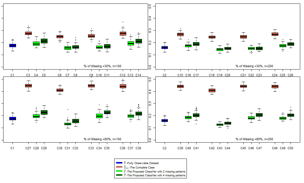
Next, we constructed our proposed classifier Γ^n\widehat{\Gamma}_{n}, given by (12), based on two different sample sizes, n=100n=100 and n=200n=200, as well as several choices for the constants a,b,a,b, and cc in (13) for each of the missing patterns. The parameters hkh_{k} and dd were selected using a data splitting approach (with a splitting ratio of 65:35 for the training set to the testing sequence) from a grid of equally spaced values hh in [0,1][0,1] and 1≤d≤dn1\leq d\leq d_{n}, based on the procedure in (9) and (10) with Gaussian kernels. Here, we took dn≈2.5​ln⁡(n)d_{n}\approx 2.5\ln(n); see Remark 2 for details and the justification for the choice of dnd_{n}. This process was repeated for 20 such random sample splits and the values of hkh_{k} and dd that minimized the average error were selected; these are denoted by h^k\widehat{h}_{k} and d^\widehat{d} which appear in (10). In addition to the proposed classifier Γ^n\widehat{\Gamma}_{n}, we also constructed the classifier based on the complete case analysis, which will be denoted by Γ^C​C\widehat{\Gamma}_{CC}, (it uses complete cases only) as well as the classifier corresponding to the case with no missing data (i.e., when all covariates are fully observable), to be denoted by Γ~n\widetilde{\Gamma}_{n}, which was proposed by Biau et al. (2005). Furthermore, our analysis here includes different missingness mechanisms such as the “Not Missing At Random” (NMAR), the “Missing At Random” (MAR), and the “Missing Completely At Random” (MCAR) scenarios. These classifiers are then used to classifying 1000 additional observations from the same underlying distribution of the data. The entire above process was repeated a total of 100 times and the average misclassification errors (over 100 Monte Carlo runs) were computed. Our findings are summarized in Table 1. The constants a,b,ca,b,c (of equation (13)) corresponding to pattern s2s_{2} are reported in columns a2,b2,c2a_{2},b_{2},c_{2} of Table 1, those corresponding to s3s_{3} are reported in columns a3,b3,c3a_{3},b_{3},c_{3}, and so on. The numbers appearing in parentheses are the standard errors of the reported misclassification errors. Figure 2 provides boxplots of the error rates of various classifiers. As shown in Table 1 and Figure 2, for both sample sizes, the error rate of the classifier Γ^n\widehat{\Gamma}_{n} is lower than that of Γ^C​C\widehat{\Gamma}_{CC} regardless of the missingness mechanism or the number of missing patterns involved. This is particularly true when the percentage of missing data is at 80%. In passing, we note that the proposed classifier Γ^n\widehat{\Gamma}_{n} can also perform better than Γ~n\widetilde{\Gamma}_{n} whenever the dependence of the missing probability mechanism on class YY (as defined via (13)) dominates its dependence on the observed and/or unobserved segments of the curves (i.e., the constant aa is orders of magnitude larger than bb and cc in (13)); see, for example, the cases C7, C8, C22, C23, C31, C32, C43, C44 in Table 1. This shows that in such cases the variable δ\delta can sometimes be a much better predictor of the class variable YY than the missing fragments of the covariate curves.

Table 1: Misclassification errors of Γ~n\widetilde{\Gamma}_{n} (fully observable data), Γ^C​C\widehat{\Gamma}_{CC} (complete case analysis), Γ^n\widehat{\Gamma}_{n} (the proposed classifier with M=3M=3 and 55 missing patterns). The numbers in parentheses are the standard errors over 100 Monte Carlo runs.
% of Missing n Missingness Mechanism a2 b2 c2 a3 b3 c3 a4 b4 c4 a5 b5 c5 Error of Γ~n\widetilde{\Gamma}_{n} Error of Γ^C​C\widehat{\Gamma}_{CC} Error of Γ^n\widehat{\Gamma}_{n} with MM=3 missing patterns Error of Γ^n\widehat{\Gamma}_{n} with MM=5 missing patterns
NMAR 0 0.95 0.13 0 0.9 1 0 1.05 0.13 0 1.2 1 C3
0.2774
(0.0179)
C4
0.1920
(0.0215)
C5
0.2124
(0.0241)
100 NMAR 2 0.01 0.8 2 0.01 0.4 2 0.01 0.3 2 0.01 0.3 C1
0.1771
(0.0178)
C6
0.2502
(0.0185)
C7
0.1581
(0.0176)
C8
0.1650
(0.0199)
MAR 1.9 0.075 0 1.9 0.075 0 2 0.085 0 2 0.085 0 C9
0.2549
(0.0187)
C10
0.1626
(0.0165)
C11
0.1700
(0.0231)
30% MCAR NA NA NA NA C12
0.2773
(0.0227)
C13
0.1939
(0.0224)
C14
0.2121
(0.0238)
NMAR 0 0.95 0.13 0 0.9 1 0 1.05 0.13 0 1.2 1 C15
0.2672
(0.0159)
C16
0.1743
(0.0157)
C17
0.1883
(0.0202)
200 NMAR 2 0.01 0.8 2 0.01 0.4 2 0.01 0.3 2 0.01 0.3 C2
0.1607
(0.0154)
C18
0.2451
(0.0137)
C19
0.1430
(0.0128)
C20
0.1517
(0.0135)
MAR 1.9 0.075 0 1.9 0.075 0 2 0.085 0 2 0.085 0 C21
0.2470
(0.0161)
C22
0.1510
(0.0147)
C23
0.1529
(0.0146)
MCAR NA NA NA NA C24
0.2686
(0.0180)
C25
0.1744
(0.0171)
C26
0.1871
(0.0159)
NMAR 0 -1.9 1.5 0 -1.45 -3 0 -2.1 1.5 0 -2 -3 C27
0.4463
(0.0184)
C28
0.1970
(0.0205)
C29
0.2284
(0.0240)
100 NMAR -5 -0.4 0.25 -4 -0.5 -0.15 -5 -0.4 0.25 -4 -0.5 -0.15 C1
0.1771
(0.0178)
C30
0.4096
(0.0158)
C31
0.1335
(0.0183)
C32
0.1554
(0.0207)
MAR 1 -3 0 -1.45 -0.95 0 0.6 -3 0 -1.9 -0.95 0 C33
0.4464
(0.0165)
C34
0.1991
(0.0244)
C35
0.2273
(0.0202)
80% MCAR NA NA NA NA C36
0.4419
(0.0187)
C37
0.1978
(0.0181)
C38
0.2178
(0.0256)
NMAR 0 -1.9 1.5 0 -1.45 -3 0 -2.1 1.5 0 -2 -3 C39
0.4410
(0.0157)
C40
0.1872
(0.0151)
C41
0.2048
(0.0227)
200 NMAR -5 -0.4 0.25 -4 -0.5 -0.15 -5 -0.4 0.25 -4 -0.5 -0.15 C2
0.1607
(0.0154)
C42
0.4087
(0.0164)
C43
0.1264
(0.0118)
C44
0.1394
(0.0150)
MAR 1 -3 0 -1.45 -0.95 0 0.6 -3 0 -1.9 -0.95 0 C45
0.4412
(0.0153)
C46
0.1824
(0.0167)
C47
0.2061
(0.0194)
MCAR NA NA NA NA C48
0.4398
(0.0179)
C49
0.1800
(0.0141)
C50
0.2058
(0.0181)
Refer to caption
Figure 2: Boxplots of the error rates of all classifiers (C1, C2, …,\dots, C50) that appear in Table 1

2.3.2 Three real datasets

In this section, we use three real-world datasets to assess the performance of the proposed classifier. In every example that follows, the smoothing parameters hkh_{k} and dd were selected using the same data splitting approach described in Section 2.3. Across these examples we see that the proposed classifier consistently performs well regardless of the proportion of fragmented curves.

Refer to caption
(a)
Refer to caption
(b)
Figure 3: (a) A sample of curves 𝓧i{\boldsymbol{\mathcal{X}}}_{i} representing CD4 cell counts measured at each visit for individuals in the HIV treatment study described in Example (A). The curves for those individuals whose data were available for every visit (complete) appear in solid black (in the top two plots) while those whose data were only available for a subset of the visits (missing) are plotted using various colored lines according to their missing pattern. The corresponding dd-dimensional vectors of projected curves, d=1,…,14d=1,\dots,14, are displayed below the original curves. (b) Distributions and proportion of class membership for each missing pattern in the utilized subset of data.

Example (A): HIV Treatment, Data from a randomized trial.

The Community Programs for Clinical Research on AIDS (CPCRA) was a program established by the National Institute of Allergy and Infectious Diseases in 1989. Seventeen research units were located in 13 cities across the US where the AIDS epidemic was most severe. Their mission was to expand the clinical research on HIV disease by conducting clinical trials (Cox et al. (1998)). The aim of one particular trial was to study the efficacy of the drugs Didanosine and Zalcitabine as secondary treatments for patients with HIV who could not tolerate or experienced disease progression despite treatment with Zidovudine, the first developed treatment for HIV. About 400 patients across 133 clinical sites were randomized to receive either Didanosine or Zalcitabine. The recruitment period lasted one year with follow-up visits at 2, 6, 12 and 18 months after enrollment in the trial (Abrams et al. (1994)).

AIDS is the most advanced stage of an HIV infection and is diagnosed in the presence of certain opportunistic infections or when an individual’s CD4 cell count decreases below 200 cells/mm3\text{mm}^{3}. An individual with an HIV diagnosis may never develop AIDS, however, expecially if HIV treatments are effective at increasing the individual’s CD4 cell count. In this context, we are interested in whether or not the participant had a previous AIDS diagnosis before entering the trial. The functional covariate 𝓧i{\boldsymbol{\mathcal{X}}}_{i} is the repeated measurement of CD4 counts for participants over the duration of the trial. The class variable yiy_{i} is coded as 0 = no previous AIDS diagnosis and 1 = previous AIDS diagnosis.

The subset of the data used in this example contains 393 observations, 53% of which are fragmented curves. There are six distinct missing data patterns observed in this dataset including the case where the data are fully observable at all visit times within the first year of the trial. A sample of CD4 cell count curves and corresponding dd-dimensional vectors of projected curves is displayed in panel (a) of Figure 3 while the distribution of each missing pattern is displayed in panel (b).

We compare the performance of our proposed classifier, Γ^n\widehat{\Gamma}_{n}, with that of the classifier based on the complete case analysis, Γ^C​C\widehat{\Gamma}_{\scriptscriptstyle CC}. To do this, the sample of n=393n=393 individuals was split into a training sequence of size n′=196n^{\prime}=196 and a testing sequence of size n−n′=197n-n^{\prime}=197. Table 2 provides the average error rates of each classifier committed on the testing sequence over 200 such sample splits with standard errors given in parenthesis as well as a visual display of classifier performance. Here we see that with over half of the observations being fragemented curves, a complete case classifier eliminates much of the available information and performs poorly compared to the classifier based on the filtered curves.

Table 2: Error rates for Γ^n\widehat{\Gamma}_{n} (the classifier based on filtered curves) and Γ^C​C\widehat{\Gamma}_{\scriptscriptstyle CC} (the complete case analysis).
[Uncaptioned image]
%\% Missing Data Γ^n\widehat{\Gamma}_{n} Γ^C​C\widehat{\Gamma}_{\scriptscriptstyle CC}
53%53\% 0.2878 0.41870.4187
(0.0233) (0.0323)(0.0323)
Refer to caption
(a)
Refer to caption
(b)
Figure 4: (a) A sample of curves 𝓧i{\boldsymbol{\mathcal{X}}}_{i} representing income-to-needs ratios for families participating in the Panel Study of Income Dynamics (PSID), described in Example (B). The curves for those families whose data were available for every survey year (complete) appear in solid black (in the top two plots) while those whose data were available in the subset of years 1998 - 2013 (missing) are plotted in red. The corresponding dd-dimensional vectors of projected curves, d=1,…,14d=1,\dots,14, are displayed below the original curves. (b) Distributions and proportion of class membership for each missing pattern in the utilized subset of the data.

Example (B): Panel Study of Income Dynamics.

The Panel Study of Income Dynamics (PSID)44 4 The collection of data used in this study was partly supported by the National Institutes of Health under grant number R01 HD069609 and the National Science Foundation under award number 1157698. is a longitudinal study of socioeconomics and health over lifetimes of participants and across generations of their families. With initial interviews in 1968, follow-up interviews were conducted annualy until 1999 and biennially thereafter. The goal of the PSID is to help researchers understand the complicated dynamics of economic, demographic, health, sociological, and psychological factors. A full description of the dataset is available at https://psidonline.isr.umich.edu. The Child Development Supplement (CDS) was added to the PSID in 1997 and studies a broad array of developmental outcomes in the 0-12 year old children of participants. The dataset used in this example is a subset of the PSID, augmented with the corresponding subset of data from the CDS.

It has been shown in the literature that an individual’s health status is positively associated with their annual income and that this association originates in childhood (see Brooks-Gunn et al. (1997), Case et al. (2002)). There is no consensus, however regarding when household income begins affecting a child’s health. This classification problem is based on a study described in Case et al. (2002) which aims to understand the effect that a household’s long-run average income has on a child’s health. The functional covariate 𝓧i{\boldsymbol{\mathcal{X}}}_{i} is the measure of income-to-needs ratios for participating families over the time period 1969 - 2013. These ratios are calculated by dividing the family’s annual household income by the poverty threshold for the corresponding family size (provided by the US Census Bureau). The class variable yiy_{i} is the self-reported health rating of the eldest child in each family, 0 = Excellent - Very Good and 1 = Good - Fair - Poor.

The subset used in this analysis consisted of n=800n=800 total observations, 8787 (11%11\%) of which were fragmented curves. There are two distinct missing patterns observed in this data, curves that are fully available for the years 1969-2013 and those that are left censored prior to 1998. A small sample of the income to needs ratio curves for families included in the subset of data and their corresponding dd-dimensional vectors of projected curves is provided in Figure 4.

We will compare the performance of our proposed classifier, Γ^n\widehat{\Gamma}_{n}, with that of the classifier based on the complete case analysis, Γ^C​C\widehat{\Gamma}_{\scriptscriptstyle CC} To do this, the sample of n=800n=800 families was split into a training sequence of size n′=400n^{\prime}=400 and a testing sequence of size n−n′=400n-n^{\prime}=400. Table 3 provides the average error rates of each classifier committed on the testing sequence over 200 such sample splits as well as a visual display of classifier performance. The standard errors are given in parenthesis. In this case we see a marginal gain by classifying using filtered curves (using Γ^n\widehat{\Gamma}_{\scriptscriptstyle n}) rather than simply performing a complete case analysis. This is likely due to the small amount of missing data which puts complete case methods on nearly equal footing with other proposed methods.

Table 3: Error rates for Γ^n\widehat{\Gamma}_{n} (the classifier based on filtered curves) and Γ^C​C\widehat{\Gamma}_{\scriptscriptstyle CC} (the complete case analysis).
[Uncaptioned image]
%\% Missing Data Γ^n\widehat{\Gamma}_{n} Γ^C​C\widehat{\Gamma}_{\scriptscriptstyle CC}
11%11\% 0.2776 0.28940.2894
(0.0146) (0.0172)(0.0172)
Refer to caption
(a)
Refer to caption
(b)
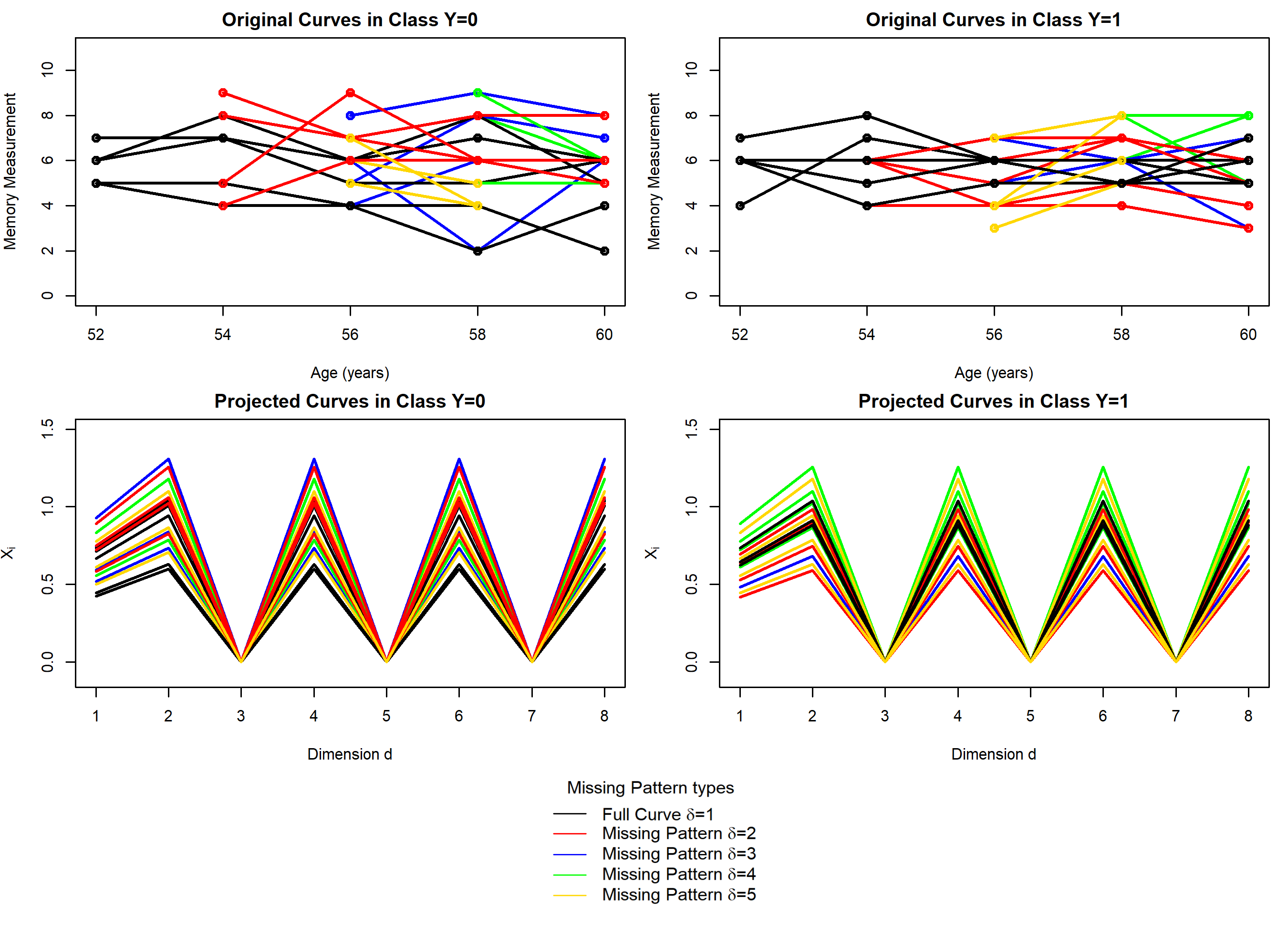
Figure 5: (a) A sample of curves 𝓧i{\boldsymbol{\mathcal{X}}}_{i} representing memory test scores measured at each visit for individuals in the Health and Retirement (HRS) study described in Example (C). The curves for those individuals whose data were available for every visit (complete) appear in solid black (in the top two plots) while those whose data were available for a subset of the visits (missing) are plotted using various colored lines according to their missing pattern. The corresponding dd-dimensional vector of the projected curves, d=1,…,8d=1,\dots,8, are displayed below the original curves. (b) Distributions and proportion of class membership for each missing pattern in the utilized subset of the data.

Example (C): Health and Retirement Study.

Advancements in medicine and health care have increased the life expectancy of individuals worldwide, resulting in the growth of the older population at an unprecedented rate. In 2015, the US Census Bureau reported that 8.5% of people worldwide were aged 65 and over and projected that the number would increase to 17% by 2050 (Wan et al. (2016)). The Health and Retirement Study (HRS), conducted by the University of Michigan and funded by the National Institute on Aging and the Social Security Administration, is a longitudinal panel study aimed at helping researchers understand the challenges and opportunities related to an aging population. The study began in 1992 with a representative cohort of 20,000 individuals aged 50 years and over and their spouses. The study is ongoing with follow-up interviews conducted biennially. Data products related to the HRS can be found at https://hrs.isr.umich.edu/data-products.

The relationship between cognitive function and survival is widely studied; and it has been shown that cognitive decline is associated with survival into old age, see for example Eun and Choi (2017) and Mueller et al. (2017). Memory is assessed for partipants in the HRS using a short-term word-recall task. At each interview, participants are given a list of 10 common nouns and asked to immediately recall as many words as they can from the list. They are asked to recall the words again 5 minutes later. The functional covariate 𝓧i{\boldsymbol{\mathcal{X}}}_{i} in this classification problem is the measured short-term memory score for participants at each visit, determined by their performance on the word-recall task. Using memory score trajectories up to the age of 60, we study the survival of individuals past the age of 65. The class variable yiy_{i} is coded as 0 = died by age 65 and 1 = survived past age 65.

So that the number of missing patterns would be more tractable, the subset of the data used in this example contains 467 observations of individuals who were enrolled in the study at age 52. Of these 467 observations, 90% are fragmented curves. There are five distinct missing patterns observed in this subset of data, including the case where the memory scores are fully observable between the ages of 52 and 60. A sample of measured memory score trajectories and corresponding dd-dimensional vectors of the projected curves is displayed in panel (a) of Figure 5 while the distribution of each missing pattern is displayed in panel (b).

To compare the performance of our proposed classifier, Γ^n\widehat{\Gamma}_{n}, with that of the classifier based on the complete case analysis, Γ^C​C\widehat{\Gamma}_{\scriptscriptstyle CC} the sample of n=467n=467 individuals was split into a training sequence of size n′=233n^{\prime}=233 and a testing sequence of size n−n′=234n-n^{\prime}=234. Table 4 provides the average error rates of each classifier committed on the testing sequence over 200 such sample splits with standard errors given in parenthesis as well as a visual display of classifier performance. One notices that the advantage of the proposed classifier Γ^n\widehat{\Gamma}_{n} over the complete case classifier seems less dramatic than expected, given the extremely large proportion of fragmented curves. This illustrates that the success of the classifier is also a function of the correlation between the outcome and the functional covariate. Though cognitive function (measured through memory) is certainly correlated with survival, it is not the strongest single predictor of survival.

Table 4: Error rates for Γ^n\widehat{\Gamma}_{n} (the classifier based on filtered curves) and Γ^C​C\widehat{\Gamma}_{\scriptscriptstyle CC} (the complete case analysis).
[Uncaptioned image]
%\% Missing Data Γ^n\widehat{\Gamma}_{n} Γ^C​C\widehat{\Gamma}_{\scriptscriptstyle CC}
90%90\% 0.3502 0.47640.4764
(0.0218) (0.0303)(0.0303)

3 Proofs

PROOF OF THEOREM 2
The proof of Part (i) is virtually the same as that of Theorem 1, whereas the proof of Part (iii) is exactly the same as that of Lemma 1 of Mojirsheibani and Shaw (2018).

The proof of Part (ii):
Let {ψ1,ψ2,…}\{\psi_{1},\psi_{2},\dots\} be a complete orthonormal basis in L2​(s)L^{2}(s), s⊂ℝs\subset\mathbb{R}, and for any 𝝌∈L2​(s)\boldsymbol{\chi}\in L^{2}(s) define the map ts:L2​(s)→ℓ2t_{s}:L^{2}(s)\to\ell_{2} by ts​(𝝌)=(⟨𝝌,ψ1⟩s,⟨𝝌,ψ2⟩s,…)t_{s}(\boldsymbol{\chi})=(\langle\boldsymbol{\chi},\psi_{1}\rangle_{s}\,,\,\langle\boldsymbol{\chi},\psi_{2}\rangle_{s}\,,\dots). Since

𝐗(k)=tk​(𝝌|sk):=(⟨𝝌,ψ1⟩sk,⟨𝝌,ψ2⟩sk,…),{\bf X}^{(k)}=t_{k}(\boldsymbol{\chi}|_{s_{k}}):=(\langle\boldsymbol{\chi},\psi_{1}\rangle_{s_{k}}\,,\,\langle\boldsymbol{\chi},\psi_{2}\rangle_{s_{k}}\,,\dots), (14)

the function ϕk​(𝐗(k))\phi_{k}({\bf X}^{(k)}) in (4) can equivalently be written as

ϕk​(𝐗(k))=ϕk​(tk​(𝝌|sk))\displaystyle\phi_{k}({\bf X}^{(k)})=\phi_{k}(t_{k}(\boldsymbol{\chi}|_{s_{k}}))
=𝔼[𝔼{YI{δ=k}−(1−Y)I{δ=k}|tk(𝝌|sk),Y}|tk(𝝌|sk)]\displaystyle~~=\mathbb{E}\left[\mathbb{E}\left\{YI\{\delta=k\}-(1-Y)I\{\delta=k\}\Big|t_{k}(\boldsymbol{\chi}|_{s_{k}}),Y\right\}\Big|t_{k}(\boldsymbol{\chi}|_{s_{k}})\right]
=𝔼[Yℙ{δ=k|tk(𝝌|sk),Y}|tk(𝝌|sk)]−𝔼[(1−Y)ℙ{δ=k|tk(𝝌|sk),Y}|tk(𝝌|sk)]\displaystyle~~=\mathbb{E}\Big[Y\,\mathbb{P}\left\{\delta=k\big|t_{k}(\boldsymbol{\chi}|_{s_{k}}),Y\right\}\Big|t_{k}(\boldsymbol{\chi}|_{s_{k}})\Big]-\mathbb{E}\Big[(1-Y)\,\mathbb{P}\left\{\delta=k\big|t_{k}(\boldsymbol{\chi}|_{s_{k}}),Y\right\}\Big|t_{k}(\boldsymbol{\chi}|_{s_{k}})\Big]~~~~~ (15)

Also, observe that with ΓB\Gamma^{\mbox{\tiny B}} as in (5),

ℙ{ΓB(𝐗(δ))=Y}\displaystyle\mathbb{P}\left\{\Gamma^{\mbox{\tiny B}}({\bf X}^{(\delta)})=Y\right\}
=ℙ⁡{ΓB​(𝐗(δ))=1,Y=1}+ℙ⁡{ΓB​(𝐗(δ))=0,Y=0}\displaystyle=\mathbb{P}\left\{\Gamma^{\mbox{\tiny B}}({\bf X}^{(\delta)})=1,Y=1\right\}+\mathbb{P}\left\{\Gamma^{\mbox{\tiny B}}({\bf X}^{(\delta)})=0,Y=0\right\}
=∑k=1M[ℙ⁡{δ=k,Y=1,ϕk​(tk​(𝝌|sk))>0}+ℙ⁡{δ=k,Y=0,ϕk​(tk​(𝝌|sk))≤0}]\displaystyle=\sum_{k=1}^{M}\Big[\mathbb{P}\big\{\delta=k,Y=1,\phi_{k}(t_{k}(\boldsymbol{\chi}|_{s_{k}}))>0\big\}+\mathbb{P}\big\{\delta=k,Y=0,\phi_{k}(t_{k}(\boldsymbol{\chi}|_{s_{k}}))\leq 0\big\}\Big]
=∑k=1M𝔼[YI{ϕk(tk(𝝌|sk))>0}⋅ℙ{δ=k|tk(𝝌|sk),Y}]\displaystyle=\sum_{k=1}^{M}\mathbb{E}\left[YI\left\{\phi_{k}(t_{k}(\boldsymbol{\chi}|_{s_{k}}))>0\right\}\cdot\mathbb{P}\left\{\delta=k\Big|t_{k}(\boldsymbol{\chi}|_{s_{k}}),Y\right\}\right]
+∑k=1M𝔼[(1−Y)I{ϕk(tk(𝝌|sk))≤0}⋅ℙ{δ=k|tk(𝝌|sk),Y}]\displaystyle~~~~~~~~~~~~~~~~~~~~+~\sum_{k=1}^{M}\mathbb{E}\left[(1-Y)I\left\{\phi_{k}(t_{k}(\boldsymbol{\chi}|_{s_{k}}))\leq 0\right\}\cdot\mathbb{P}\left\{\delta=k\Big|t_{k}(\boldsymbol{\chi}|_{s_{k}}),Y\right\}\right]
=∑k=1M𝔼[I{ϕk(tk(𝝌|sk))>0}⋅𝔼(Y⋅ℙ{δ=k|tk(𝝌|sk),Y}|tk(𝝌|sk))]\displaystyle=\sum_{k=1}^{M}\mathbb{E}\left[I\Big\{\phi_{k}(t_{k}(\boldsymbol{\chi}|_{s_{k}}))>0\Big\}\cdot\mathbb{E}\left(Y\cdot\mathbb{P}\left\{\delta=k\Big|t_{k}(\boldsymbol{\chi}|_{s_{k}}),Y\right\}\bigg|t_{k}(\boldsymbol{\chi}|_{s_{k}})\right)\right]
+∑k=1M𝔼[I{ϕk(tk(𝝌|sk))≤0}⋅𝔼((1−Y)⋅ℙ{δ=k|tk(𝝌|sk),Y}|tk(𝝌|sk))]\displaystyle~~~~~~~~~~~~~~~~~~~~+~\sum_{k=1}^{M}\mathbb{E}\left[I\Big\{\phi_{k}(t_{k}(\boldsymbol{\chi}|_{s_{k}}))\leq 0\Big\}\cdot\mathbb{E}\left((1-Y)\cdot\mathbb{P}\left\{\delta=k\Big|t_{k}(\boldsymbol{\chi}|_{s_{k}}),Y\right\}\bigg|t_{k}(\boldsymbol{\chi}|_{s_{k}})\right)\right]
=∑k=1M𝔼[max{𝔼(Y⋅ℙ{δ=k|tk(𝝌|sk),Y}|tk(𝝌|sk)),\displaystyle=\sum_{k=1}^{M}\mathbb{E}\Bigg[\max\Bigg\{\mathbb{E}\left(Y\cdot\mathbb{P}\left\{\delta=k\Big|t_{k}(\boldsymbol{\chi}|_{s_{k}}),Y\right\}\bigg|t_{k}(\boldsymbol{\chi}|_{s_{k}})\right)\,,
𝔼((1−Y)⋅ℙ{δ=k|tk(𝝌|sk),Y}|tk(𝝌|sk))}],\displaystyle~~~~~~~~~~~~~~~~~~~~~~~~\mathbb{E}\left((1-Y)\cdot\mathbb{P}\left\{\delta=k\Big|t_{k}(\boldsymbol{\chi}|_{s_{k}}),Y\right\}\bigg|t_{k}(\boldsymbol{\chi}|_{s_{k}})\right)\Bigg\}\Bigg],

where the last equality above follows from the representation of ϕk​(tk​(𝝌|sk))\phi_{k}(t_{k}(\boldsymbol{\chi}|_{s_{k}})) in (15). However, using the fact that ℙ{δ=k|tk(𝝌|sk),Y}=𝔼[ℙ{δ=k|𝝌|sk,Y}|tk(𝝌|sk),Y]\mathbb{P}\left\{\delta=k\big|t_{k}(\boldsymbol{\chi}|_{s_{k}}),Y\right\}=\mathbb{E}\left[\mathbb{P}\left\{\delta=k\big|\,\boldsymbol{\chi}|_{s_{k}},Y\right\}\big|t_{k}(\boldsymbol{\chi}|_{s_{k}}),Y\right], we can write

ℙ{ΓB(𝐗(δ))=Y}\displaystyle\mathbb{P}\left\{\Gamma^{\mbox{\tiny B}}({\bf X}^{(\delta)})=Y\right\}
=∑k=1M𝔼[max{𝔼(𝔼[Y⋅ℙ{δ=k|𝝌|sk,Y}|tk(𝝌|sk),Y]|tk(𝝌|sk)),\displaystyle=\sum_{k=1}^{M}\mathbb{E}\Bigg[\max\Bigg\{\mathbb{E}\left(\mathbb{E}\Big[Y\cdot\mathbb{P}\left\{\delta=k\Big|\boldsymbol{\chi}|_{s_{k}},Y\right\}\Big|t_{k}(\boldsymbol{\chi}|_{s_{k}}),Y\Big]\bigg|t_{k}(\boldsymbol{\chi}|_{s_{k}})\right)\,,
𝔼(𝔼[(1−Y)⋅ℙ{δ=k|𝝌|sk,Y}|tk(𝝌|sk),Y]|tk(𝝌|sk))}]\displaystyle~~~~~~~~~~~~~~~~~~~~~~~~\mathbb{E}\left(\mathbb{E}\Big[(1-Y)\cdot\mathbb{P}\left\{\delta=k\Big|\boldsymbol{\chi}|_{s_{k}},Y\right\}\Big|t_{k}(\boldsymbol{\chi}|_{s_{k}}),Y\Big]\bigg|t_{k}(\boldsymbol{\chi}|_{s_{k}})\right)\Bigg\}\Bigg]
=∑k=1M𝔼⁡[max⁡{𝔼⁡(Y​ℙ​{δ=k​|𝝌|sk,Y}|tk​(𝝌|sk)),𝔼⁡((1−Y)​ℙ​{δ=k​|𝝌|sk,Y}|tk​(𝝌|sk))}]\displaystyle=\sum_{k=1}^{M}\mathbb{E}\Bigg[\max\Bigg\{\mathbb{E}\left(Y\mathbb{P}\left\{\delta=k\Big|\boldsymbol{\chi}|_{s_{k}},Y\right\}\bigg|t_{k}(\boldsymbol{\chi}|_{s_{k}})\right)\,,~\mathbb{E}\left((1-Y)\mathbb{P}\left\{\delta=k\Big|\boldsymbol{\chi}|_{s_{k}},Y\right\}\bigg|t_{k}(\boldsymbol{\chi}|_{s_{k}})\right)\Bigg\}\Bigg]
=∑k=1M𝔼[max{𝔼[𝔼(Yℙ{δ=k|𝝌|sk,Y}|𝝌|sk)|tk(𝝌|sk)],\displaystyle=\sum_{k=1}^{M}\mathbb{E}\Bigg[\max\Bigg\{\mathbb{E}\left[\mathbb{E}\left(Y\mathbb{P}\left\{\delta=k\Big|\boldsymbol{\chi}|_{s_{k}},Y\right\}\bigg|\boldsymbol{\chi}|_{s_{k}}\right)\bigg|t_{k}(\boldsymbol{\chi}|_{s_{k}})\right]\,,
𝔼[𝔼((1−Y)ℙ{δ=k|𝝌|sk,Y}|𝝌|sk)|tk(𝝌|sk)]}]\displaystyle~~~~~~~~~~~~~~~~~~~~~~~~\mathbb{E}\left[\mathbb{E}\left((1-Y)\mathbb{P}\left\{\delta=k\Big|\boldsymbol{\chi}|_{s_{k}},Y\right\}\bigg|\boldsymbol{\chi}|_{s_{k}}\right)\bigg|t_{k}(\boldsymbol{\chi}|_{s_{k}})\right]\Bigg\}\Bigg]
≤∑k=1M𝔼[𝔼(max{𝔼(Yℙ{δ=k|𝝌|sk,Y}|𝝌|sk),\displaystyle\leq\,\sum_{k=1}^{M}\mathbb{E}\Bigg[\mathbb{E}\Bigg(\max\Bigg\{\mathbb{E}\left(Y\mathbb{P}\left\{\delta=k\Big|\boldsymbol{\chi}|_{s_{k}},Y\right\}\bigg|\boldsymbol{\chi}|_{s_{k}}\right)\,,
𝔼((1−Y)ℙ{δ=k|𝝌|sk,Y}|𝝌|sk)}|tk(𝝌|sk))],(by Jensen’s inequality)\displaystyle~~~~~~~~~~~~~~~~~~~\mathbb{E}\left((1-Y)\,\mathbb{P}\left\{\delta=k\Big|\boldsymbol{\chi}|_{s_{k}},Y\right\}\bigg|\boldsymbol{\chi}|_{s_{k}}\right)\Bigg\}\Bigg|t_{k}(\boldsymbol{\chi}|_{s_{k}})\Bigg)\Bigg],~\mbox{(by Jensen's inequality)}
=∑k=1M𝔼⁡[max⁡{𝔼⁡(Y​ℙ​{δ=k​|𝝌|sk,Y}​|𝝌|sk),𝔼⁡((1−Y)​ℙ​{δ=k​|𝝌|sk,Y}​|𝝌|sk)}]\displaystyle=\sum_{k=1}^{M}\mathbb{E}\Bigg[\max\Bigg\{\mathbb{E}\left(Y\mathbb{P}\left\{\delta=k\Big|\boldsymbol{\chi}|_{s_{k}},Y\right\}\bigg|\boldsymbol{\chi}|_{s_{k}}\right),\,\mathbb{E}\left((1-Y)\mathbb{P}\left\{\delta=k\Big|\boldsymbol{\chi}|_{s_{k}},Y\right\}\bigg|\boldsymbol{\chi}|_{s_{k}}\right)\Bigg\}\Bigg]
=ℙ{Γ0B(𝝌(δ))=Y},\displaystyle=\mathbb{P}\left\{\Gamma_{0}^{\mbox{\tiny B}}(\boldsymbol{\chi}^{(\delta)})=Y\right\},

i.e., ℙ{ΓB(𝐗(δ))≠Y}≥ℙ{Γ0B(𝝌(δ))≠Y}\mathbb{P}\left\{\Gamma^{\mbox{\tiny B}}({\bf X}^{(\delta)})\neq Y\right\}\geq\,\mathbb{P}\left\{\Gamma_{0}^{\mbox{\tiny B}}(\boldsymbol{\chi}^{(\delta)})\neq Y\right\}, where Γ0B​(𝝌(δ))\Gamma_{0}^{\mbox{\tiny B}}(\boldsymbol{\chi}^{(\delta)}) is the optimal classifier defined in (2); see Theorem 1. To complete the proof, it is sufficient to show that the map tkt_{k} in (14) is one-to-one (and thus invertible). But, observe that for 𝐮,𝐯∈L2​(sk){\bf u},{\bf v}\in L^{2}(s_{k}), we have tk​(𝐮−𝐯)=0t_{k}({\bf u}-{\bf v})=0 if and only if 𝐮−𝐯=0{\bf u}-{\bf v}=0 (by the completeness of the basis {ψ1,ψ2,…}\{\psi_{1},\psi_{2},\dots\}); the result now follows since tk​(𝐮)−tk​(𝐯)=tk​(𝐮−𝐯)t_{k}({\bf u})-t_{k}({\bf v})=t_{k}({\bf u}-{\bf v}).

□\Box

PROOF OF THEOREM 3
We recall that if δ=k\delta=k then 𝐗(d,k){\bf X}^{(d,k)} is the observed dd-dim covariate, where k=1,…,Mk=1,\dots,M. This means that when δ=k\delta=k, a classifier is any function of the form gd,k:ℝd→{0,1}g_{d,k}:\mathbb{R}^{d}\to\{0,1\}. Therefore the general classifier, denoted by Γd\Gamma^{d}, can always be written in the form

Γd(𝐗(d,δ)):=∑k=1MI{δ=k}⋅gd,k(𝐗(d,k)).\Gamma^{d}({\bf X}^{(d,\delta)}):=\sum_{k=1}^{M}I\{\delta=k\}\cdot g_{d,k}({\bf X}^{(d,k)}). (16)

Now, for k=1,…,Mk=1,\dots,M, define the functions rk(𝐱,y)=ℙ{δ=k|𝐗(d,k)=𝐱,Y=y},y=0,1,r_{k}({\bf x},y)=\mathbb{P}\left\{\delta=k\,\big|\,{\bf X}^{(d,k)}={\bf x},Y=y\right\},~~y=0,1, and ηk​(𝐱)=ℙ⁡{Y=1|𝐗(d,k)=𝐱}=𝔼⁡[Y|𝐗(d,k)=𝐱],\eta_{k}({\bf x})=\mathbb{P}\left\{Y=1\,\big|\,{\bf X}^{(d,k)}={\bf x}\right\}\,=\,\mathbb{E}\left[Y\big|{\bf X}^{(d,k)}={\bf x}\right], and observe that the function ϕd,k\phi_{d,k} in (6) can be written as

ϕd,k​(𝐗(d,k))\displaystyle\phi_{d,k}({\bf X}^{(d,k)}) =\displaystyle= 𝔼{𝔼[(2Y−1)I{δ=k}|𝐗(d,k),Y]|𝐗(d,k)},\displaystyle\mathbb{E}\left\{\mathbb{E}\left[(2Y-1)I\{\delta=k\}\,\Big|\,{\bf X}^{(d,k)},\,Y\right]\Big|{\bf X}^{(d,k)}\right\}, (17)
=\displaystyle= 𝔼[(2Y−1)ℙ{δ=k|𝐗(d,k),Y}|𝐗(d,k)]\displaystyle\mathbb{E}\left[(2Y-1)\mathbb{P}\{\delta=k\big|{\bf X}^{(d,k)},\,Y\}\,\Big|\,{\bf X}^{(d,k)}\right]
=\displaystyle= 𝔼⁡[(2​Y−1)​(Y⋅rk​(𝐗(d,k),1)+(1−Y)​rk​(𝐗(d,k),0))|𝐗(d,k)]\displaystyle\mathbb{E}\left[(2Y-1)\Big(Y\cdot r_{k}({\bf X}^{(d,k)},1)+(1-Y)r_{k}({\bf X}^{(d,k)},0)\Big)\,\Big|\,{\bf X}^{(d,k)}\right]
=\displaystyle= 𝔼⁡[Y⋅rk​(𝐗(d,k),1)+(Y−1)⋅rk​(𝐗(d,k),0)|𝐗(d,k)],(because Y2=Y)\displaystyle\mathbb{E}\left[Y\cdot r_{k}({\bf X}^{(d,k)},1)+(Y-1)\cdot r_{k}({\bf X}^{(d,k)},0)\,\Big|\,{\bf X}^{(d,k)}\right]\,,~\mbox{(because $Y^{2}$=$Y$)}
=\displaystyle= ηk​(𝐗(d,k))​rk​(𝐗(d,k),1)+(ηk​(𝐗(d,k))−1)​rk​(𝐗(d,k),0).\displaystyle\eta_{k}({\bf X}^{(d,k)})r_{k}({\bf X}^{(d,k)},1)+\Big(\eta_{k}({\bf X}^{(d,k)})-1\Big)r_{k}({\bf X}^{(d,k)},0).

Therefore, the classifier ΓB,d\Gamma^{\mbox{\tiny B},d} in (7) can be written as

ΓB,d(𝐗(d,δ))=∑k=1MI{δ=k}⋅I{ηk(𝐗(d,k))rk(𝐗(d,k),1)+(ηk(𝐗(d,k))−1)rk(𝐗(d,k),0)>0},\Gamma^{\mbox{\tiny B},d}({\bf X}^{(d,\delta)})=\sum_{k=1}^{M}I\{\delta=k\}\cdot I\left\{\eta_{k}({\bf X}^{(d,k)})r_{k}({\bf X}^{(d,k)},1)+\Big(\eta_{k}({\bf X}^{(d,k)})-1\Big)r_{k}({\bf X}^{(d,k)},0)>0\right\},

and this can be used to write

ℙ{ΓB,d(𝐗(d,δ))=Y}\displaystyle\mathbb{P}\left\{\Gamma^{\mbox{\tiny B},d}({\bf X}^{(d,\delta)})=Y\right\}
=∑k=1Mℙ{Y=1,δ=k,[ϕd,k(𝐗(d,k))>0]}+∑k=1Mℙ{Y=0,δ=k,[ϕd,k(𝐗(d,k))≤0]}\displaystyle~~=\sum_{k=1}^{M}\mathbb{P}\left\{Y=1,\delta=k,[\phi_{d,k}({\bf X}^{(d,k)})>0]\right\}+\sum_{k=1}^{M}\mathbb{P}\left\{Y=0,\delta=k,[\phi_{d,k}({\bf X}^{(d,k)})\leq 0]\right\}
:=∑k=1Mπk​1+∑k=1Mπk​0,(say).\displaystyle~~:=\sum_{k=1}^{M}\pi_{k1}+\sum_{k=1}^{M}\pi_{k0}\,,~~(\mbox{say}).

But

πk​1\displaystyle\pi_{k1} =\displaystyle= 𝔼[I{Y=1}⋅I{ϕd,k(𝐗(d,k))>0}⋅ℙ{δ=k|𝐗(d,k),Y}]\displaystyle\mathbb{E}\Big[I\{Y=1\}\cdot I\left\{\phi_{d,k}({\bf X}^{(d,k)})>0\right\}\cdot\mathbb{P}\left\{\delta=k\big|{\bf X}^{(d,k)},Y\right\}\Big]
=\displaystyle= 𝔼[I{ϕd,k(𝐗(d,k))>0}⋅rk(𝐗(d,k),1)⋅𝔼[I{Y=1}|𝐗(d,k)]]\displaystyle\mathbb{E}\Big[I\left\{\phi_{d,k}({\bf X}^{(d,k)})>0\right\}\cdot r_{k}({\bf X}^{(d,k)},1)\cdot\mathbb{E}\big[I\{Y=1\}\big|{\bf X}^{(d,k)}\big]\Big]
=\displaystyle= 𝔼[I{ϕd,k(𝐗(d,k))>0}⋅rk(𝐗(d,k),1)⋅ηk(𝐗(d,k))].\displaystyle\mathbb{E}\Big[I\left\{\phi_{d,k}({\bf X}^{(d,k)})>0\right\}\cdot r_{k}({\bf X}^{(d,k)},1)\cdot\eta_{k}({\bf X}^{(d,k)})\Big].

Also, similar arguments yield πk​0=𝔼[I{ϕd,k(𝐗(d,k))≤0}⋅rk(𝐗(d,k),0)⋅(1−ηk(𝐗(d,k)))].\pi_{k0}=\mathbb{E}\big[I\left\{\phi_{d,k}({\bf X}^{(d,k)})\leq 0\right\}\cdot r_{k}({\bf X}^{(d,k)},0)\cdot\big(1-\eta_{k}({\bf X}^{(d,k)})\big)\big]. Thus, we have

ℙ{ΓB,d(𝐗(d,δ))=Y}\displaystyle\mathbb{P}\{\Gamma^{\mbox{\tiny B},d}({\bf X}^{(d,\delta)})=Y\} =\displaystyle= ∑k=1M(𝔼[I{ϕd,k(𝐗(d,k))>0}⋅rk(𝐗(d,k),1)⋅ηk(𝐗(d,k))]\displaystyle\sum_{k=1}^{M}\Bigg(\mathbb{E}\Big[I\left\{\phi_{d,k}({\bf X}^{(d,k)})>0\right\}\cdot r_{k}({\bf X}^{(d,k)},1)\cdot\eta_{k}({\bf X}^{(d,k)})\Big]
+𝔼[I{ϕd,k(𝐗(d,k))≤0}⋅rk(𝐗(d,k),0)⋅(1−ηk(𝐗(d,k)))]).\displaystyle~~~+\mathbb{E}\Big[I\left\{\phi_{d,k}({\bf X}^{(d,k)})\leq 0\right\}\cdot r_{k}({\bf X}^{(d,k)},0)\cdot\Big(1-\eta_{k}({\bf X}^{(d,k)})\Big)\Big]\Bigg).

Furthermore, for any other classifier Γd​(𝐗(d,δ))\Gamma^{d}({\bf X}^{(d,\delta)}) given by (16), it is not difficult to see that

ℙ{Γd(𝐗(d,δ))=Y}\displaystyle\mathbb{P}\{\Gamma^{d}({\bf X}^{(d,\delta)})=Y\} =\displaystyle= ∑k=1M(𝔼[I{gd,k(𝐗(d,k))=1}⋅rk(𝐗(d,k),1)⋅ηk(𝐗(d,k))]\displaystyle\sum_{k=1}^{M}\Bigg(\mathbb{E}\Big[I\left\{g_{d,k}({\bf X}^{(d,k)})=1\right\}\cdot r_{k}({\bf X}^{(d,k)},1)\cdot\eta_{k}({\bf X}^{(d,k)})\Big]
+𝔼[I{gd,k(𝐗(d,k))=0}⋅rk(𝐗(d,k),0)⋅(1−ηk(𝐗(d,k)))]).\displaystyle~~~+\mathbb{E}\Big[I\left\{g_{d,k}({\bf X}^{(d,k)})=0\right\}\cdot r_{k}({\bf X}^{(d,k)},0)\cdot\Big(1-\eta_{k}({\bf X}^{(d,k)})\Big)\Big]\Bigg).

Therefore,

ℙ{ΓB,d(𝐗(d,δ))≠Y}−ℙ{Γd(𝐗(d,δ))≠Y}\displaystyle\mathbb{P}\{\Gamma^{\mbox{\tiny B},d}({\bf X}^{(d,\delta)})\neq Y\}-\mathbb{P}\{\Gamma^{d}({\bf X}^{(d,\delta)})\neq Y\}
=∑k=1M𝔼[(I{ϕd,k(𝐗(d,k))>0}−I{gd,k(𝐗(d,k))=1})⋅rk(𝐗(d,k),1)⋅ηk(𝐗(d,k))]\displaystyle=\sum_{k=1}^{M}\mathbb{E}\Big[\Big(I\left\{\phi_{d,k}({\bf X}^{(d,k)})>0\right\}-I\left\{g_{d,k}({\bf X}^{(d,k)})=1\right\}\Big)\cdot r_{k}({\bf X}^{(d,k)},1)\cdot\eta_{k}({\bf X}^{(d,k)})\Big]
+∑k=1M𝔼[(I{ϕd,k(𝐗(d,k))≤0}−I{gd,k(𝐗(d,k))=0})⋅rk(𝐗(d,k),0)⋅(1−ηk(𝐗(d,k)))]\displaystyle~~+\sum_{k=1}^{M}\mathbb{E}\Big[\Big(I\left\{\phi_{d,k}({\bf X}^{(d,k)})\leq 0\right\}-I\left\{g_{d,k}({\bf X}^{(d,k)})=0\right\}\Big)\cdot r_{k}({\bf X}^{(d,k)},0)\cdot\big(1-\eta_{k}({\bf X}^{(d,k)})\big)\Big]~~
=∑k=1M𝔼[I{gd,k(𝐗(d,k))≠I{ϕd,k(𝐗(d,k))>0}}\displaystyle=\sum_{k=1}^{M}\mathbb{E}\Bigg[I\bigg\{g_{d,k}({\bf X}^{(d,k)})\neq I\left\{\phi_{d,k}({\bf X}^{(d,k)})>0\right\}\bigg\} (18)
×|rk(𝐗(d,k),1)⋅ηk(𝐗(d,k))−rk(𝐗(d,k),0)⋅(1−ηk(𝐗(d,k)))|]\displaystyle~~~~~~~~~~~~~~~~~~\times\bigg|r_{k}({\bf X}^{(d,k)},1)\cdot\eta_{k}({\bf X}^{(d,k)})-r_{k}({\bf X}^{(d,k)},0)\cdot\big(1-\eta_{k}({\bf X}^{(d,k)})\big)\bigg|\Bigg]
≥0,\displaystyle\geq 0,

where (18) follows from the definitions of ΓB,d\Gamma^{\mbox{\tiny B},d} and Γd\Gamma^{d} in conjunction with the expression in (17).

□\Box

In order to prove Theorem 4, we first state a number of lemmas. In what follows, we use the following notation:

ℛm​(d,h1,…,hM)\displaystyle\mathcal{R}_{m}(d,h_{1},\dots,h_{M}) =\displaystyle= ℙ⁡{Γmd​(𝐗(d,δ))≠Y|𝔻m}\displaystyle\mathbb{P}\left\{\Gamma_{m}^{d}({\bf X}^{(d,\delta)})\neq Y\big|\mathbb{D}_{m}\right\} (19)
ℛ^m,ℓ​(d,h1,…,hM)\displaystyle\widehat{\mathcal{R}}_{m,\ell}(d,h_{1},\dots,h_{M}) =\displaystyle= ℓ−1∑i:(𝐗(δi),Yi,δi)∈𝔻ℓI{Ωi(m,d,h1,…,hM)},\displaystyle\ell^{-1}\sum_{i:~{(\bf X}^{(\delta_{i})},Y_{i},\delta_{i})\in\mathbb{D}_{\ell}}I\big\{\Omega_{i}(m,d,h_{1},\dots,h_{M})\big\}, (20)

where Γmd​(𝐗(d,δ))\Gamma_{m}^{d}({\bf X}^{(d,\delta)}) and Ωi​(m,d,h1,…,hM)\Omega_{i}(m,d,h_{1},\dots,h_{M}) are as in (9) and (11), respectively.

Lemma 1

Let ℛ^m,ℓ\widehat{\mathcal{R}}_{m,\ell} and ℛm\mathcal{R}_{m} be as in (20) and (19). If ℓ−1​log⁡|ℋn|→0\ell^{-1}\log|\mathcal{H}_{n}|\to 0 and ℓ−1​log⁡dn→0\ell^{-1}\log d_{n}\to 0, where |ℋn||\mathcal{H}_{n}| is the cardinality of the set ℋn\mathcal{H}_{n}, then, as n→∞n\to\infty,

sup1≤d≤dn,h1,…,hM∈ℋn|ℛ^m,ℓ​(d,h1,…,hM)−ℛm​(d,h1,…,hM)|\displaystyle\sup_{1\leq d\leq d_{n}\,,\,h_{1},\dots,h_{M}\in\mathcal{H}_{n}~}\left|\widehat{\mathcal{R}}_{m,\ell}(d,h_{1},\dots,h_{M})-\mathcal{R}_{m}(d,h_{1},\dots,h_{M})\right| ⟶a.s.\displaystyle\longrightarrow^{\mbox{a.s.}} 0.\displaystyle 0\,.

PROOF OF LEMMA 1
First observe that for any given constant β>0\beta>0,

ℙ{sup1≤d≤dn,h1,…,hM∈ℋn|ℛ^m,ℓ(d,h1,…,hM)−ℛm(d,h1,…,hM)|>β}\displaystyle\mathbb{P}\left\{\sup_{1\leq d\leq d_{n}\,,\,h_{1},\dots,h_{M}\in\mathcal{\mathcal{H}}_{n}~}\left|\widehat{\mathcal{R}}_{m,\ell}(d,h_{1},\dots,h_{M})-\mathcal{R}_{m}(d,h_{1},\dots,h_{M})\right|>\beta\right\}
≤∑1≤d≤dn∑h1,…,hM∈ℋnℙ{|ℛ^m,ℓ(d,h1,…,hM)−ℛm(d,h1,…,hM)|>β}\displaystyle~\leq~\sum_{1\leq d\leq d_{n}}\sum_{~h_{1},\dots,h_{M}\in\mathcal{H}_{n}}\mathbb{P}\left\{\left|\widehat{\mathcal{R}}_{m,\ell}(d,h_{1},\dots,h_{M})-\mathcal{R}_{m}(d,h_{1},\dots,h_{M})\right|>\beta\right\}
≤dn​|ℋn|M​sup1≤d≤dnsuph1,…,hM∈ℋn𝔼⁡[ℙ⁡{|ℛ^m,ℓ​(d,h1,…,hM)−ℛm​(d,h1,…,hM)|>β|𝔻m}]\displaystyle~\leq~d_{n}|\mathcal{H}_{n}|^{M}\sup_{1\leq d\leq d_{n}}\sup_{h_{1},\dots,h_{M}\in\mathcal{H}_{n}}\mathbb{E}\left[\mathbb{P}\left\{\left|\widehat{\mathcal{R}}_{m,\ell}(d,h_{1},\dots,h_{M})-\mathcal{R}_{m}(d,h_{1},\dots,h_{M})\right|>\beta\bigg|\mathbb{D}_{m}\right\}\right]~~~

where |ℋn||\mathcal{H}_{n}| is the cardinality of the set ℋn\mathcal{H}_{n}. But, with Ωi​(m,d,h1,…,hM)\Omega_{i}(m,d,h_{1},\dots,h_{M}) as in (11),

ℙ⁡{|ℛ^m,ℓ​(d,h1,…,hM)−ℛm​(d,h1,…,hM)|>β|𝔻m}\displaystyle\mathbb{P}\left\{\left|\widehat{\mathcal{R}}_{m,\ell}(d,h_{1},\dots,h_{M})-\mathcal{R}_{m}(d,h_{1},\dots,h_{M})\right|>\beta\,\Big|\,\mathbb{D}_{m}\right\}
=ℙ{|ℓ−1∑i:(𝐗(δi),Yi,δi)∈𝔻ℓI{Ωi(m,d,h1,…,hM)}−ℙ{Ω1(m,d,h1,…,hM)}|>β|𝔻m}\displaystyle~~=~\mathbb{P}\Bigg\{\bigg|\ell^{-1}\sum_{i:~{(\bf X}^{(\delta_{i})},Y_{i},\delta_{i})\in\mathbb{D}_{\ell}}I\big\{\Omega_{i}(m,d,h_{1},\dots,h_{M})\big\}-\mathbb{P}\big\{\Omega_{1}(m,d,h_{1},\dots,h_{M})\big\}\bigg|>\beta\,\Bigg|\,\mathbb{D}_{m}\Bigg\}~~~~
≤2​e−2​ℓ​β2,(by Hoeffding’s inequality),\displaystyle~~\leq~2\,e^{-2\ell\beta^{2}},~~~~~~\mbox{(by Hoeffding's inequality),}

which does not depend on 𝔻m\mathbb{D}_{m} or any of the parameters d,h1,…,hMd,h_{1},\dots,h_{M}. Therefore

ℙ{sup1≤d≤dn,h1,…,hM∈ℋn|ℛ^m,ℓ(d,h1,…,hM)−ℛm(d,h1,…,hM)|>β}\displaystyle\mathbb{P}\left\{\sup_{1\leq d\leq d_{n}\,,\,h_{1},\dots,h_{M}\in\mathcal{H}_{n}~}\left|\widehat{\mathcal{R}}_{m,\ell}(d,h_{1},\dots,h_{M})-\mathcal{R}_{m}(d,h_{1},\dots,h_{M})\right|>\beta\right\} ≤\displaystyle\leq 2​dn​|ℋn|M​e−2​ℓ​β2.\displaystyle 2\,d_{n}|\mathcal{H}_{n}|^{M}e^{-2\ell\beta^{2}}.

Furthermore, the conditions of Lemma 1 imply that ∑n=1∞dn|ℋn|Me−ℓβ2/2<∞\sum_{n=1}^{\infty}d_{n}|\mathcal{H}_{n}|^{M}e^{-\ell\beta^{2}/2}<\infty. The result now follows from an application of the Borel-Cantelli lemma.

□\Box

Lemma 2

Let Γ^n​(𝐗(d^,δ))\widehat{\Gamma}_{n}({\bf X}^{(\widehat{d},\delta)}) be the classifier in (12). Also, let ℛ^m,ℓ\widehat{\mathcal{R}}_{m,\ell} and ℛm\mathcal{R}_{m} be as in (20) and (19). Then

ℙ⁡{Γ^n​(𝐗(d^,δ))≠Y|𝔻n}−inf1≤d≤dn,h1,…,hM∈ℋnℛm​(d,h1,…,hM)\displaystyle\mathbb{P}\left\{\widehat{\Gamma}_{n}({\bf X}^{(\widehat{d},\delta)})\neq Y\Big|\mathbb{D}_{n}\right\}~-\inf_{1\leq d\leq d_{n}\,,\,h_{1},\dots,h_{M}\in\mathcal{H}_{n}~}\mathcal{R}_{m}(d,h_{1},\dots,h_{M})
≤2​sup1≤d≤dn,h1,…,hM∈ℋn|ℛ^m,ℓ​(d,h1,…,hM)−ℛm​(d,h1,…,hM)|.\displaystyle~~~~~~\leq~~2~\sup_{1\leq d\leq d_{n}\,,\,h_{1},\dots,h_{M}\in\mathcal{H}_{n}~}\left|\widehat{\mathcal{R}}_{m,\ell}(d,h_{1},\dots,h_{M})-\mathcal{R}_{m}(d,h_{1},\dots,h_{M})\right|.

PROOF of LEMMA 2
The proof of this lemma, which is similar to that of Lemma 8.2 of Devroye et al (1996), is straightforward and will not be given here. □\Box

Lemma 3

Let ΓB,d​(𝐗(d,δ))\Gamma^{\mbox{\tiny B},d}({\bf X}^{(d,\delta)}) be the classifier defined via (7) and (6). Also, let gd,kg_{d,k} in the definition of the classifier Γd​(𝐗(d,δ))\Gamma^{d}({\bf X}^{(d,\delta)}) in (16) be of the form gd,k(𝐗(d,k))=I{Gd,k(𝐗(d,k))>0}g_{d,k}({\bf X}^{(d,k)})=I\{G_{d,k}({\bf X}^{(d,k)})>0\} for some function Gd,k:ℝd→[−1,1]G_{d,k}:\mathbb{R}^{d}\to[-1,1]. Then

ℙ{Γd(𝐗(d,δ))≠Y}−ℙ{ΓB,d(𝐗(d,δ))≠Y}\displaystyle\mathbb{P}\left\{\Gamma^{d}({\bf X}^{(d,\delta)})\neq Y\right\}-\mathbb{P}\left\{\Gamma^{\mbox{\tiny B},d}({\bf X}^{(d,\delta)})\neq Y\right\} ≤\displaystyle\leq ∑k=1M𝔼​|ϕd,k​(𝐗(d,k))−Gd,k​(𝐗(d,k))|,\displaystyle\sum_{k=1}^{M}\mathbb{E}\Big|\phi_{d,k}({\bf X}^{(d,k)})-G_{d,k}({\bf X}^{(d,k)})\Big|\,,

where ΓB,d​(𝐗(d,δ))\Gamma^{\mbox{\tiny B},d}({\bf X}^{(d,\delta)}) and ϕd,k​(𝐗(d,k))\phi_{d,k}({\bf X}^{(d,k)}) are as in (7) and (6), respectively.

PROOF OF LEMMA 3
The expression in (18) in the proof of Theorem 3 shows that in view of (17) one has

ℙ{Γd(𝐗(d,δ))≠Y}−ℙ{ΓB,d(𝐗(d,δ))≠Y}\displaystyle\mathbb{P}\left\{\Gamma^{d}({\bf X}^{(d,\delta)})\neq Y\right\}-\mathbb{P}\left\{\Gamma^{\mbox{\tiny B},d}({\bf X}^{(d,\delta)})\neq Y\right\}
≤∑k=1M𝔼(I{gd,k(𝐗(d,k))≠I{ϕd,k(𝐗(d,k))>0}}×|ϕd,k(𝐗(d,k))|).\displaystyle~~~~~\leq~\sum_{k=1}^{M}\mathbb{E}\bigg(I\Big\{g_{d,k}({\bf X}^{(d,k)})\neq I\left\{\phi_{d,k}({\bf X}^{(d,k)})>0\right\}\Big\}\times\Big|\phi_{d,k}({\bf X}^{(d,k)})\Big|\bigg)\,.

Given the definition of gd,k​(𝐗(d,k))g_{d,k}({\bf X}^{(d,k)}) in the statement of the lemma, it is straightforward to see that on the set {gd,k(𝐗(d,k))≠I{ϕd,k(𝐗(d,k))>0}}\big\{g_{d,k}({\bf X}^{(d,k)})\neq I\left\{\phi_{d,k}({\bf X}^{(d,k)})>0\right\}\big\}, one has

𝔼(I{gd,k(𝐗(d,k))≠I{ϕd,k(𝐗(d,k))>0}}×|ϕd,k(𝐗(d,k))|)\displaystyle\mathbb{E}\bigg(I\Big\{g_{d,k}({\bf X}^{(d,k)})\neq I\left\{\phi_{d,k}({\bf X}^{(d,k)})>0\right\}\Big\}\times\Big|\phi_{d,k}({\bf X}^{(d,k)})\Big|\bigg) ≤\displaystyle\leq 𝔼​|ϕd,k​(𝐗(d,k))−Gd,k​(𝐗(d,k))|,\displaystyle\mathbb{E}\Big|\phi_{d,k}({\bf X}^{(d,k)})-G_{d,k}({\bf X}^{(d,k)})\Big|,

which completes the proof of the lemma.

□\Box

The following result is an immediate corollary to Lemma 3.

Corollary 1

Let ΓB,d​(𝐗(d,δ))\Gamma^{\mbox{\tiny B},d}({\bf X}^{(d,\delta)}) be the classifier defined via (7) and (6). Also, for k=1,…,Mk=1,\dots,M, let Gm,d,k​(𝐗(d,k))G_{m,d,k}({\bf X}^{(d,k)}) be any sample-based version of the function Gd,k​(𝐗(d,δ))G_{d,k}({\bf X}^{(d,\delta)}) that appears in Lemma 3, based on the training sample 𝔻m\mathbb{D}_{m}, and consider the classifier

Γ~m(𝐗(d,δ))=∑k=1MI{δ=k}⋅gm,d,k(𝐗(d,k)),\widetilde{\Gamma}_{m}({\bf X}^{(d,\delta)})=\sum_{k=1}^{M}I\{\delta=k\}\cdot g_{m,d,k}({\bf X}^{(d,k)}),

where gm,d,k(𝐗(d,k))=I{Gm,d,k(𝐗(d,k))>0}g_{m,d,k}({\bf X}^{(d,k)})=I\left\{G_{m,d,k}({\bf X}^{(d,k)})>0\right\}. Then

ℙ{Γ~m(𝐗(d,δ))≠Y|𝔻m}−ℙ{ΓB,d(𝐗(d,δ))≠Y}\displaystyle\mathbb{P}\left\{\widetilde{\Gamma}_{m}({\bf X}^{(d,\delta)})\neq Y\Big|\mathbb{D}_{m}\right\}-\mathbb{P}\left\{\Gamma^{\mbox{\tiny B},d}({\bf X}^{(d,\delta)})\neq Y\right\} ≤\displaystyle\leq ∑k=1M𝔼⁡[|ϕd,k​(𝐗(d,k))−Gm,d,k​(𝐗(d,k))||𝔻m].\displaystyle\sum_{k=1}^{M}\mathbb{E}\left[\Big|\phi_{d,k}({\bf X}^{(d,k)})-G_{m,d,k}({\bf X}^{(d,k)})\Big|\bigg|\mathbb{D}_{m}\right].

The proof of Corollary 1 is the same as that of Lemma 3 and is obtained by conditioning on the training sample 𝔻m\mathbb{D}_{m}.

□\Box

The next lemma is a well-known result on the performance of the L1L^{1}-norm of kernel regression estimators.

Lemma 4

[Devroye et al (1996, Theorem 1); Györfi et al (2002, Lemma 23.9).]
Let (U,𝐕)∈[−B,B]×ℝd(U,{\bf V})\in[-B,B]\times\mathbb{R}^{d}, where B<∞B<\infty, and let ϕ⁡(𝐯)=𝔼⁡[U|𝐕=𝐯]\phi({\bf v})=\mathbb{E}[U|{\bf V}={\bf v}] be the regression function. Let 𝔻n={(U1,𝐕1),…,(Un,𝐕n)}\mathbb{D}_{n}=\{(U_{1},{\bf V}_{1}),\dots,(U_{n},{\bf V}_{n})\} be the data (iid), where (Ui,𝐕i)=i​i​d(U,𝐕)(U_{i},{\bf V}_{i})\stackrel{{\scriptstyle iid}}{{=}}(U,{\bf V}), and define ϕ^n(𝐯)=∑i=1nUi𝒦((𝐯−𝐕i)/hn)/{n𝔼[𝒦(𝐯−𝐕)/hn)]},\widehat{\phi}_{n}({\bf v})=\sum_{i=1}^{n}U_{i}\mathcal{K}(({\bf v}-{\bf V}_{i})/{h_{n}})\,\big/\,\left\{n\,\mathbb{E}\left[\mathcal{K}({\bf v}-{\bf V})/h_{n})\right]\right\}, where 𝒦:ℝd→ℝ+\mathcal{K}:\mathbb{R}^{d}\to\mathbb{R}_{+} is regular. If hn→0h_{n}\to 0 and n​hnd→∞nh_{n}^{d}\to\infty, as n→∞n\to\infty, then for any distribution of (U,𝐕)(U,{\bf V}), any ϵ>0\epsilon>0, and nn large enough,

ℙ{𝔼[|ϕ^n(𝐕)−ϕ(𝐕)||𝔻n]>ϵ}≤e−nϵ2/(8Bρ)2,\mathbb{P}\left\{\mathbb{E}\left[\big|\widehat{\phi}_{n}({\bf V})-\phi({\bf V})\big|\,\Big|\,\mathbb{D}_{n}\right]>\epsilon\right\}\leq e^{-n\epsilon^{2}/(8B\rho)^{2}},

where ρ≡ρ⁡(𝒦)\rho\equiv\rho(\mathcal{K}) is a positive constant depending on the kernel 𝒦\mathcal{K} only.

PROOF OF THEOREM 4
Let ΓB,d​(𝐗(d,δ))\Gamma^{\mbox{\tiny B},d}({\bf X}^{(d,\delta)}) and ΓB​(𝐗(δ))\Gamma^{\mbox{\tiny B}}({\bf X}^{(\delta)}) be as in (7) and (5), and observe that in view of part (iii) of Theorem 2 one has

ℙ{ΓB,d(𝐗(d,δ))≠Y}−ℙ{ΓB(𝐗(δ))≠Y}\displaystyle\mathbb{P}\{\Gamma^{\mbox{\tiny B},d}({\bf X}^{(d,\delta)})\neq Y\}-\mathbb{P}\{\Gamma^{\mbox{\tiny B}}({\bf X}^{(\delta)})\neq Y\}
≤∑k=1M𝔼|𝔼[(2Y−1)I{δ=k}|𝐗(k)]−𝔼[(2Y−1)I{δ=k}|𝐗(d,k)]|,\displaystyle~~\leq~\sum_{k=1}^{M}\mathbb{E}\bigg|\mathbb{E}\Big[(2Y-1)I\{\delta=k\}\Big|{\bf X}^{(k)}\Big]-\mathbb{E}\Big[(2Y-1)I\{\delta=k\}\Big|{\bf X}^{(d,k)}\Big]\bigg|, (21)

which follows upon taking φk​(𝐗(k))\varphi_{k}({\bf X}^{(k)}), that appears in part (iii) of Theorem 2, to be the same as the right side of (6). Here, as before, 𝐗(k)=(X1(k),X2(k),…){\bf X}^{(k)}=(X_{1}^{(k)},X_{2}^{(k)},\,\dots) and 𝐗(d,k)=(X1(k),…,Xd(k)){\bf X}^{(d,k)}=(X_{1}^{(k)},\dots,X_{d}^{(k)}). Let Sd(k)=𝔼[(2Y−1)I{δ=k}|𝐗(d,k)]S_{d}^{(k)}=\mathbb{E}\big[(2Y-1)I\{\delta=k\}\big|{\bf X}^{(d,k)}\big] and S∞(k)=𝔼[(2Y−1)I{δ=k}|𝐗(k)]S_{\infty}^{(k)}=\mathbb{E}\big[(2Y-1)I\{\delta=k\}\big|{\bf X}^{(k)}\big], and observe that for any k=1,…,Mk=1,\dots,M and any d1<d2d_{1}<d_{2}, one has 𝔼[Sd2(k)|X1(k),…,Xd1(k)]\mathbb{E}\big[S_{d_{2}}^{(k)}\big|X_{1}^{(k)},\dots,X_{d_{1}}^{(k)}\big] =a.s.Sd1(k)\stackrel{{\scriptstyle\mbox{\tiny a.s.}}}{{=}}S_{d_{1}}^{(k)}. Furthermore, supd≥1|Sd(k)|≤1\sup_{d\geq 1}\big|S_{d}^{(k)}\big|\leq 1. In other words, {Sd(k),d=1,2,…}\{S_{d}^{(k)},d=1,2,\dots\} is a martingale with respect to the increasing sequence of σ\sigma-fields, σ⁡(X1(k),…,Xd(k))\sigma(X_{1}^{(k)},\dots,X_{d}^{(k)}). Invoking the martingale convergence theorem (see, for example, Sec. 1.3 of Hall and Heyde (1980)), and arguing as in Biau et al. (2005), we find Sd(k)→a.s.S∞(k)S_{d}^{(k)}\to^{a.s.}S_{\infty}^{(k)}, as d→∞d\to\infty. This fact together with the bound in (21) and an application of the dominated convergence theorem yield ℙ{ΓB,d(𝐗(d,δ))≠Y}−ℙ{ΓB(𝐗(δ))≠Y}→0\mathbb{P}\{\Gamma^{\mbox{\tiny B},d}({\bf X}^{(d,\delta)})\neq Y\}-\mathbb{P}\{\Gamma^{\mbox{\tiny B}}({\bf X}^{(\delta)})\neq Y\}\to 0, as d→∞d\to\infty. Consequently, for every ϵ>0\epsilon>0, and nn sufficiently large, there is a dϵ∈[1,dn]d_{\epsilon}\in[1,d_{n}] such that ℙ{ΓB,d(𝐗(d,δ))≠Y}−ℙ{ΓB(𝐗(δ))≠Y}≤ϵ\mathbb{P}\{\Gamma^{\mbox{\tiny B},d}({\bf X}^{(d,\delta)})\neq Y\}-\mathbb{P}\{\Gamma^{\mbox{\tiny B}}({\bf X}^{(\delta)})\neq Y\}\leq\epsilon holds for all d≥dϵd\geq d_{\epsilon} (recall dn→∞d_{n}\to\infty as n→∞n\to\infty). Therefore, for any h~k≡h~​(n)∈ℋn\widetilde{h}_{k}\equiv\widetilde{h}(n)\in\mathcal{H}_{n}, k=1,…,nk=1,\dots,n, satisfying the conditions of Theorem 4, any ϵ>0\epsilon>0, and nn large enough, one has

ℙ{Γ^n(𝐗(d^,δ))≠Y|𝔻n}−ℙ{ΓB(𝐗(δ))≠Y}\displaystyle\mathbb{P}\left\{\widehat{\Gamma}_{n}({\bf X}^{(\widehat{d},\delta)})\neq Y\,\Big|\,\mathbb{D}_{n}\right\}-\mathbb{P}\left\{\Gamma^{\mbox{\tiny B}}({\bf X}^{(\delta)})\neq Y\right\}
=ℙ⁡{Γ^n​(𝐗(d^,δ))≠Y|𝔻n}−inf1≤d≤dn,h1,…,hM∈ℋnℛm​(d,h1,…,hM)\displaystyle~~~~~~~~=~\mathbb{P}\left\{\widehat{\Gamma}_{n}({\bf X}^{(\widehat{d},\delta)})\neq Y\,\big|\,\mathbb{D}_{n}\right\}~-\inf_{1\leq d\leq d_{n}\,,\,h_{1},\dots,h_{M}\in\mathcal{H}_{n}~}\mathcal{R}_{m}(d,h_{1},\dots,h_{M})
+inf1≤d≤dn,h1,…,hM∈ℋn{ℛm(d,h1,…,hM)−ℙ{ΓB,d(𝐗(d,δ))≠Y}\displaystyle~~~~~~~~~~~~~~+~\inf_{1\leq d\leq d_{n}\,,\,h_{1},\dots,h_{M}\in\mathcal{H}_{n}}\bigg\{\mathcal{R}_{m}(d,h_{1},\dots,h_{M})-\mathbb{P}\{\Gamma^{\mbox{\tiny B},d}({\bf X}^{(d,\delta)})\neq Y\}
+ℙ{ΓB,d(𝐗(d,δ))≠Y}}−ℙ{ΓB(𝐗(δ))≠Y}\displaystyle~~~~~~~~~~~~~~~~~~~~~~~~~~~~~~~~~~~~~~~~~~~~~~~+~\mathbb{P}\{\Gamma^{\mbox{\tiny B},d}({\bf X}^{(d,\delta)})\neq Y\}\bigg\}-~\mathbb{P}\left\{\Gamma^{\mbox{\tiny B}}({\bf X}^{(\delta)})\neq Y\right\}
≤ℙ⁡{Γ^n​(𝐗(d^,δ))≠Y|𝔻n}−inf1≤d≤dn,h1,…,hM∈ℋnℛm​(d,h1,…,hM)\displaystyle~~~~~~~~\leq~\mathbb{P}\left\{\widehat{\Gamma}_{n}({\bf X}^{(\widehat{d},\delta)})\neq Y\,\big|\,\mathbb{D}_{n}\right\}~-\inf_{1\leq d\leq d_{n}\,,\,h_{1},\dots,h_{M}\in\mathcal{H}_{n}~}\mathcal{R}_{m}(d,h_{1},\dots,h_{M})
+ℛm(dϵ,h~1,…,h~M)−ℙ{ΓB,dϵ(𝐗(dϵ,δ))≠Y}\displaystyle~~~~~~~~~~~~~~+~\mathcal{R}_{m}(d_{\epsilon},\widetilde{h}_{1},\dots,\widetilde{h}_{M})-\mathbb{P}\{\Gamma^{\mbox{\tiny B},d_{\epsilon}}({\bf X}^{(d_{\epsilon},\delta)})\neq Y\}
+ϵ\displaystyle~~~~~~~~~~~~~~+~\epsilon (22)

Now, in view of lemmas 1 and 2, as n→∞n\to\infty, we have

ℙ{Γ^n(𝐗(d^,δ))≠Y|𝔻n}−inf1≤d≤dn,h1,…,hM∈ℋnℛm(d,h1,…,hM)⟶a.s.0,\mathbb{P}\left\{\widehat{\Gamma}_{n}({\bf X}^{(\widehat{d},\delta)})\neq Y\,\big|\,\mathbb{D}_{n}\right\}~-\inf_{1\leq d\leq d_{n}\,,\,h_{1},\dots,h_{M}\in\mathcal{H}_{n}~}\mathcal{R}_{m}(d,h_{1},\dots,h_{M})\longrightarrow^{\mbox{\small a.s.}}0, (23)

Next, define

ϕ~m,d,hk​(𝐱)=ϕ^m,d,hk​(𝐱)m⋅𝔼​[𝒦k​(𝐱−𝐗(d,k)hk)],\widetilde{\phi}_{m,d,h_{k}}({\bf x})=\frac{\widehat{\phi}_{m,d,h_{k}}({\bf x})}{m\cdot\mathbb{E}\left[\mathcal{K}_{k}\left(\frac{{\bf x}-{\bf X}^{(d,k)}}{h_{k}}\right)\right]}\,,

where ϕ^m,d,hk​(𝐱)\widehat{\phi}_{m,d,h_{k}}({\bf x}) is as in (8), and observe that the classifier Γmd\Gamma_{m}^{d} in (9) can alternatively be written as Γmd(𝐗(d,δ))=∑k=1MI{δ=k}I{ϕ~m,d,hk(𝐗(d,k))>0}\Gamma_{m}^{d}({\bf X}^{(d,\delta)})=\sum_{k=1}^{M}I\{\delta=k\}I\big\{\widetilde{\phi}_{m,d,h_{k}}({\bf X}^{(d,k)})>0\big\}. Therefore, by Corollary 1,

ℛm(dϵ,h~1,…,h~M)−ℙ{ΓB,dϵ(𝐗(dϵ,δ))≠Y}\displaystyle\mathcal{R}_{m}(d_{\epsilon},\widetilde{h}_{1},\dots,\widetilde{h}_{M})-\mathbb{P}\{\Gamma^{\mbox{\tiny B},d_{\epsilon}}({\bf X}^{(d_{\epsilon},\delta)})\neq Y\} ≤\displaystyle\leq ∑i=1M𝔼⁡[|ϕdϵ,k​(𝐗(dϵ,k))−ϕ~m,dϵ,h~k​(𝐗(dϵ,k))||𝔻m]\displaystyle\sum_{i=1}^{M}\mathbb{E}\left[\Big|\phi_{d_{\epsilon},k}({\bf X}^{(d_{\epsilon},k)})-\widetilde{\phi}_{m,d_{\epsilon},\widetilde{h}_{k}}({\bf X}^{(d_{\epsilon},k)})\Big|\bigg|\mathbb{D}_{m}\right] (24)
⟶a.s.0,asn→∞,\displaystyle\longrightarrow^{\mbox{\small a.s.}}0,~~\mbox{as}~n\to\infty,
(by Lemma 4 and the Borel-Cantelli lemma)

where ϕdϵ,k\phi_{d_{\epsilon},k} is given by (6). Therefore, in view of (22), (23), and (24), for any ϵ>0\epsilon>0,

limn→∞[ℙ{Γ^n(𝐗(d^,δ))≠Y|𝔻n}−ℙ{ΓB(𝐗(δ))≠Y}]\displaystyle\lim_{n\to\infty}\left[\mathbb{P}\left\{\widehat{\Gamma}_{n}({\bf X}^{(\widehat{d},\delta)})\neq Y\,\Big|\,\mathbb{D}_{n}\right\}-\mathbb{P}\left\{\Gamma^{\mbox{\tiny B}}({\bf X}^{(\delta)})\neq Y\right\}\right] ≤\displaystyle\leq ϵ,\displaystyle\epsilon\,,

almost surely. This completes the proof of Theorem 4.

□\Box

References

Abraham, C.,

Biau, G., Cadre, B., 2006. On the kernel rule for functional classification. AISM 58, 619-633.

Abrams, D.,

Goldma,n A., Launer, C., Korvick, J., Neaton J., et al. (1994). A comparitive trial of didanosine or zalcitabine after treatment with zidovudine in patients with human immunodeficiency virus infection. NEJM, 10, 657-662.

Alonso, A,

Casado, D., López-Pintado, S., Romo, J., (2014). Robust functional supervised classification for time series. J. Classification 31, 3, 325-350.

Berlinet, A.,

Biau, G., Rouviere, L., 2008. Functional classification with wavelets. Annales de l’Institut de statistique de l’université de Paris 52, 61-80.

Biau, G.,

Bunea, F., Wegkamp, M.H., 2005. Functional classification in hilbert spaces. IEEE T. Inform. Theory. 51, 2163-2172.

Brooks-Gunn, J.,

Duncan, G., Maritato, N. (1997). Poor families, poor outcomes: the well-being of children and youth. In: Duncan GJ, Brooks-Gunn J, editors. Consequences of Growing up Poor. Russell Sage Foundation; New York, pp. 1–17.

Bugni,

F., 2012. Specification test for missing functional data. Economet. Theor. 28, 959-1002.

Cai, T.,

Hall, P., 2006. Prediction in functional linear regression. Annals of Statistics, 34, 2159-2179.

Case, A.,

Lubtosky, D., Paxson, C., 2002. Economic status and health in childhood: the origins of the gradient. Am. Econ. Rev. 92, 1308-1334.

Cérou, F.,

Guyader, A., 2006. Nearest neighbor classification in infinite dimensions. ESAIM-Probab. Stat. 10,340-355.

Chang, C.,

Chen, Y., Ogden, R.T., 2014. Functional data classification: a wavelet approach. Computation. Stat. 29, 1497-1513.

Cox, L.,

Rouff, J., Svendsen, K., Markowitz, M., Abrams, D., CPCRA (1998). Community advisory boards: their role in AIDS clinical trials. Health and Social Work, 4, 290-297.

Cuevas, A.,

Febrero, M., Fraiman, R., 2007. Robust estimation and classification for functional data via projection-based depth notions. Computation. Stat. 22, 481-496.

Dai, X.,

Müller, H.-G., 2017. Optimal Bayes classifiers for functional data and density ratios. Biometrika 104, 3, 545-560.

Delaigle, A.

Hall, P., 2013. Classification using censored functional data. J Am Stat Assoc 108, 1269-1283.

Delaigle, A.

Hall, P., 2012. Achieving near perfect classification for functional data. J Royal Stat Soc B 74, Part 2, 267-286.

Delaigle, A.,

Hall, P., Bathia, N., 2012. Componentwise classification and clustering for functional data. Biometrika 99, 299-313.

Devroye, L.,

Györfi, L., Lugosi, G., 1996. A Probabilistic Theory of Pattern Recognition. Springer, New York.

Eun, H.,

and Choi, M. (2017). Relationship between structural changes of brain and cognitive function and survival rate in alzheimer’s disease patients. Alzheimers Dement, 13, pp 1367.

Ferraty, F.,

Vieu, P., (2006). Nonparametric functional data analysis, Theory and practice. Springer, New York.

Ferraty, F.,

Vieu, P., 2003. Curves discrimination: a nonparametric functional approach. Comput. Stat. Data An. 4, 161-173.

Györfi, L.,

Kohler, M., Krzyzak, A., Walk, H., 2002. A distribution-free theory of non-parametric regression. Springer, New York.

Hall, P.,

Heyde, C.C., 1980. Martingale limit theory and its application. Academic Press.

Hall, P.,

Horowitz, J.L., 2007. Methodology and convergence rates for functional linear regression. Annals of Statistics, 35, 70-91.

Hall, P.,

Poskitt, D.S., Presnell, B., 2001. Functional data-analytic approach to signal discrimination. Technometrics 43, 1-9.

He, W.,

Goodkind, D., Kowal, P. U.S. Census Bureau, International Population Reports, P95/16-1, An Aging World: 2015, U.S. Government Publishing Office, Washington, DC, 2016.

Kraus, D.,

2015. Components and completion of partially observed functional data. J. R. Stat. Soc. B. 77, 777-801.

Leng, X.,

Müller, H.-G., 2006. Classification using functional data analysis for temporal gene expression data. Bioinformatics 22, 68-76.

López-Pintado,

S., Romo, J., 2006. Depth-based classification for functional data, in DIMACS Ser. Discrete M. 72, 103-120.

Meister, A.,

2016. Optimal classification and nonparametric regression for functional data. Bernoulli 22, 1729-1744.

Mojirsheibani, M.,

Shaw, C., 2018. Classification with incomplete functional covariates. Stat. & Probab. Lett. 139, 40-46.

Mosler, K.,

Mozharovskyi, P., 2017. Fast DD-classification of functional data. Stat. Papers 58, 1055-1089.

Mueller, C.,

Stubbs, B., Banerji, S., Stewart, R., Perera, G. (2017). Concomitant use of anticholinergic medication attenuates benefits of cholinesterase inhibitors in alzheimer’s disease: a large cohort study of survival and cognitive function. Alzheimers Dement, 13, pp 851.

Rachdi, M.,

Vieu, P., 2007. Nonparametric regression for functional data: Automatic smoothing parameter selection. J. Stat. Plan. Infer. 137, 2784-2801.

Sansone, G.,

1969. Orthogonal Functions. Interscience, New York.

Song, J.J.,

Deng, W., Lee, H.-J., Kwon, D., 2008. Optimal classification for time-course gene expression data using functional data analysis. Comput. Biol. Chem. 32, 426-432.

van Buuren,

S., Groothuis-Oudshoorn, K. (2011). mice: Multivariate Imputation by Chained Equations in R. J. of Stat. Software, 45, 1-67.

Yao, F.,

Müller, H.-G., 2010. Functional quadratic regression. Biometrika, 97, 49-64.

Zygmund, A.,

1959. Trigonometric Series I. Cambridge Univ. Press.