跳到论文正文
W Papers独立论文阅读器 arXiv:1810.07128 论文正文 计算阅读时间 · 0%
引用这篇论文根据当前论文元数据生成,正式投稿前建议核对。


License: arXiv.org perpetual non-exclusive license
arXiv:1810.07128v4 [stat.ML] 25 Oct 2019

Sen Na, Zhuoran Yang, Zhaoran Wang, and Mladen Kolar

High-dimensional Varying Index Coefficient Models via Stein’s Identity

Sen Na senna@uchicago.edu Affiliation: Department of Statistics Affiliation: University of Chicago Affiliation: Chicago, IL 60637, USA    Zhuoran Yang zy6@princeton.edu Affiliation: Department of Operations Research and Financial Engineering Affiliation: Princeton University Affiliation: Princeton, NJ 08544, USA    Zhaoran Wang zhaoran.wang@northwestern.edu Affiliation: Department of Industrial Engineering and Management Sciences Affiliation: Northwestern University Affiliation: Evanston, IL 60208, USA    Mladen Kolar mkolar@chicagobooth.edu Affiliation: The University of Chicago Booth School of Business Affiliation: Chicago, IL 60637, USA
Abstract

We study the parameter estimation problem for a varying index coefficient model in high dimensions. Unlike the most existing works that iteratively estimate the parameters and link functions, based on the generalized Stein’s identity, we propose computationally efficient estimators for the high-dimensional parameters without estimating the link functions. We consider two different setups where we either estimate each sparse parameter vector individually or estimate the parameters simultaneously as a sparse or low-rank matrix. For all these cases, our estimators are shown to achieve optimal statistical rates of convergence (up to logarithmic terms in the low-rank setting). Moreover, throughout our analysis, we only require the covariate to satisfy certain moment conditions, which is significantly weaker than the Gaussian or elliptically symmetric assumptions that are commonly made in the existing literature. Finally, we conduct extensive numerical experiments to corroborate the theoretical results.

††heading: 20 2019 1– 10/18; Revised 5/19 10/19 18-705††shortheadings: High-dimensional Varying Index Coefficient Models via Stein’s Identity / Na, Yang, Wang, and Kolar††firstpage: 1††editor: Kenji Fukumizu
keywords
high-dimensional estimation, semiparametric modeling, Stein’s identity, varying index coefficient model

1 Introduction

We consider the problem of estimating parameters in a high-dimensional varying index coefficient model with following form

y=∑j=1d2zj⋅fj​(⟨𝒙,𝜷j⋆⟩)+ϵ,\displaystyle y=\sum_{j=1}^{d_{2}}z_{j}\cdot f_{j}(\langle{\bm{x}},\bm{\beta}^{\star}_{j}\rangle)+\epsilon, (1)

where yy is response variable, 𝒙=(x1,…,xd1)⊤∈ℝd1{\bm{x}}=(x_{1},\ldots,x_{d_{1}})^{\top}\in\mathbb{R}^{d_{1}} and 𝒛=(z1,…,zd2)⊤∈ℝd2{\bm{z}}=(z_{1},\ldots,z_{d_{2}})^{\top}\in\mathbb{R}^{d_{2}} are given covariates, and ϵ\epsilon is random noise with 𝔼[ϵ∣𝒙,𝒛]=0\mathbb{E}[\epsilon\mid{\bm{x}},{\bm{z}}]=0. For j∈[d2]j\in[d_{2}]11 1 For any integer dd, we denote [d]={1,2,…,d}[d]=\{1,2,...,d\}., 𝜷j⋆=(βj​1⋆,…,βj​d1⋆)⊤\bm{\beta}^{\star}_{j}=(\beta_{j1}^{\star},\ldots,\beta_{jd_{1}}^{\star})^{\top} are the coefficient vectors, that is parameters, which vary with different covariates zjz_{j}, and fj​(⋅)f_{j}(\cdot) are unknown nonparametric link functions. For identification purposes, we can always permute 𝜷j⋆\bm{\beta}^{\star}_{j} and multiply by a scalar such that

𝜷j⋆∈{𝜷∈ℝd1:∥𝜷∥2=1 and β1>0},j=1,…,d2.\bm{\beta}^{\star}_{j}\in\{\bm{\beta}\in\mathbb{R}^{d_{1}}:\|\bm{\beta}\|_{2}=1\text{ and }\beta_{1}>0\},\quad j=1,\ldots,d_{2}. (2)

All further restrictions on parameters will only be considered under (2).

Model (1) has been introduced by Ma and Song 2015 as a flexible generalization of a number of well studied semiparametric statistical models (Xue and Wang 2012, see also). When zj=1z_{j}=1 for all j∈[d2]j\in[d_{2}], the model reduces to the additive single-index model (Chen 1991; Carroll et al. 1997), which can also be viewed as a two-layer neural network with d2d_{2} hidden nodes. When d1=1d_{1}=1 and 𝜷j⋆=1\bm{\beta}^{\star}_{j}=1 for j=1,…,d2j=1,\ldots,d_{2}, the model (1) reduces to the varying coefficient model proposed in Cleveland et al. 1991 and Hastie and Tibshirani 1993, with wide applications in scientific areas such as economics and medical science (Fan and Zhang 2008). Varying coefficient models allow the coefficients of 𝒛{\bm{z}} to be smooth functions of 𝒙{\bm{x}}, thus incorporating nonlinear interactions between 𝒙{\bm{x}} and 𝒛{\bm{z}}. Model (1) is also easily interpreted in real applications because it inherits features from both single-index model and varying coefficient model, while being able to capture complex multivariate nonlinear structure.

Our focus is on the case when the dimension of 𝒙{\bm{x}} is high, which makes estimation of the coefficients difficult. Existing procedures estimate the unknown functions and coefficients iteratively. First, with the signal parameters {𝜷j⋆}j∈[d2]\{\bm{\beta}^{\star}_{j}\}_{j\in[d_{2}]} fixed, one estimates the functions {fj​(⋅)}j∈[d2]\{f_{j}(\cdot)\}_{j\in[d_{2}]} using a nonparametric method, such as local polynomial estimator. Next, using the estimated link functions, one re-estimates the coefficients. While the global minimizer has desirable properties (see Xue and Wang 2012 and Ma and Song 2015 and the references therein), the loss function is usually nonconvex and it is computationally intractable to obtain the global optima. For high-dimensional single-index models (d2=1d_{2}=1 and 𝒛=1{\bm{z}}=1), when the distribution of 𝒙{\bm{x}} is known, the signal parameter can be estimated directly by fitting Lasso (Tibshirani 1996). Such an estimator is shown to achieve minimax-optimal statistical rate of convergence (Plan and Vershynin 2016; Plan et al. 2017). Thus, the following question naturally arises:

Is it possible to estimate signal parameters {𝛃j⋆}j∈[d2]\{\bm{\beta}^{\star}_{j}\}_{j\in[d_{2}]} in (1) with both statistical accuracy and computational efficiency?

In this work, we provide a positive answer to above question. Specifically, we focus on the problem of estimating the parameter matrix 𝑩⋆=(𝜷1⋆,…,𝜷d2⋆)∈ℝd1×d2\bm{B}^{\star}=(\bm{\beta}^{\star}_{1},\ldots,\bm{\beta}^{\star}_{d_{2}})\in\mathbb{R}^{d_{1}\times d_{2}} in the high-dimensional setting where the sample size is much smaller than d1×d2d_{1}\times d_{2} and 𝑩⋆\bm{B}^{\star} is either sparse or low-rank. We utilize the score functions and the generalized Stein’s identity (Stein 1972; Stein et al. 2004) to estimate the unknown coefficients through a regularized least-square regression problem, without learning the unknown functions {fj​(⋅)}j∈[d2]\{f_{j}(\cdot)\}_{j\in[d_{2}]}. We prove that the estimators achieve (near) optimal statistical rates of convergence under weak moment conditions, which make our procedure suitable for heavy-tailed data, using a careful truncation argument. Finally, our estimator can be computed as a solution to a convex optimization problem.

Main Contributions. Our contributions are three-fold. First, we propose a computationally efficient estimation procedure for the varying index coefficient model in high dimensions. Different from existing work, our approach does not need to estimate the unknown functions {fj}j∈[d2]\{f_{j}\}_{j\in[d_{2}]}. Second, when 𝑩⋆\bm{B}^{\star} is sparse, we prove that the proposed estimator achieves the optimal statistical rate of convergence, while when 𝑩⋆\bm{B}^{\star} is low-rank, our estimator is shown to be near-optimal (up to a logarithmic factor). Finally, we provide thorough numerical experiments with both synthetic and real data to back up our theories.

Related Work. There is a plethora of literature on the varying coefficient model, first proposed in Cleveland et al. 1991 and Hastie and Tibshirani 1993, where the coefficients are modeled as nonparametric functions of 𝒙{\bm{x}}. See Fan and Zhang 2008 for a detailed review. Xia and Li 1999, Fan et al. 2003, and Xue and Wang 2012 considered model in (1) with 𝜷j⋆=𝜷⋆\bm{\beta}^{\star}_{j}=\bm{\beta}^{\star} for all j∈[d2]j\in[d_{2}] and estimated it with standard nonparametric techniques. Ma and Song 2015 proposed model (1) and developed a profile least-square approach to estimate the coefficients. Unfortunately, the estimator is defined as a solution to a constrained optimization problem with nonconvex objective function that can be hard to globally optimize in practice. This should be contrasted to estimators that are based on solving convex optimization problems.

Another related line of research is on the high-dimensional single-index model (SIM) with sparse coefficient vector, which is a special case of model (1). Most of the existing results require either knowing the distribution of 𝒙{\bm{x}} or strong assumptions on the link functions. Specifically, Thrampoulidis et al. 2015, Neykov et al. 2016, Plan and Vershynin 2016, and Plan et al. 2017 all showed that when 𝒙{\bm{x}} is a standard Gaussian and the link function satisfies certain conditions, Lasso estimators could also work for SIM with the same theoretical guarantee as if the link function is not present. To relax the Gaussian assumption, Goldstein et al. 2018 proposed a modified Lasso-type estimator when 𝒙{\bm{x}} has an elliptically symmetric distribution. Moreover, using the generalized Stein’s identity, Yang et al. 2017 proposed a soft-thresholding estimator for SIM when the distribution of 𝒙{\bm{x}} is known, and Na and Kolar 2018 proposed estimators for single-index volatility model. Our work can be viewed as the extension of this work from two aspects. First, as mentioned before, our model in (1) includes the single-index model considered in Yang et al. 2017 as a special case, which can be recovered by letting d2=1d_{2}=1 and 𝒛=1{\bm{z}}=1. In comparison, our model contains d2d_{2} unknown signal vectors {𝜷j⋆}j∈[d2]\{\bm{\beta}^{\star}_{j}\}_{j\in[d_{2}]}, where d2d_{2} itself can be large compared to the sample size. As we will show later, when the parameter matrix 𝑩⋆\bm{B}^{\star} has a certain low-dimensional structure, such as being sparse or low rank, we construct efficient estimators that enjoy sharp statistical rates of convergence even when d2d_{2} is large and {zj}j∈[d2]\{z_{j}\}_{j\in[d_{2}]} are dependent, heavy-tailed. Second, from the methodology perspective, our estimators are based on combining the first-order Stein’s identity and the dependence structure of the covariate 𝒛{\bm{z}}, which is a novel observation in index models and generalizes the method in Yang et al. 2017 for SIM. In particular, we extract the information of the parameter matrix 𝑩⋆\bm{B}^{\star} via multiplying the response yy by the score function of 𝒙{\bm{x}} and the covariate 𝒛{\bm{z}} adjusted by its precision matrix (see (5)). When 𝒛{\bm{z}} has independent components, our procedure for estimating each single sparse vector 𝜷j⋆\bm{\beta}^{\star}_{j} is equivalent to fitting d2d_{2} SIMs using the procedure proposed in Yang et al. 2017. However, even having independent {zj}j∈[d2]\{z_{j}\}_{j\in[d_{2}]}, their method fails when estimating 𝑩⋆\bm{B}^{\star} as a whole with either low-rank or sparse structure, since they only have one coefficient and cannot deal with varying coefficient models without accounting for 𝒛{\bm{z}} in Stein’s identity. Furthermore, to handle dependence structure of 𝒛{\bm{z}} in general, we construct suitable precision matrix estimators for heavy-tailed variable in either low or high dimensions based on the CLIME procedure (Cai et al. 2011) and the soft truncation technique, which is of independent interests. Besides aforementioned related literature, a sequence of work (Zhu et al. 2006; Jiang and Liu 2014; Zhang et al. 2017; Lin et al. 2017; Lin et al. 2018) applied the sliced inverse regression (SIR) technique on high-dimensional SIM, which is generalized from Li 1991. But all these works require the distribution of 𝒙{\bm{x}} to be Gaussian or elliptical. To resolve this limitation, Babichev and Bach 2018 incorporated SIR with both first-order and second-order score function when fitting a low-dimensional index model, while the high-dimensional analysis is not included.

Furthermore, our work is also related to the study of additive index model, which is more challenging than (1), and there is very much work in this direction. Most existing work focuses on estimating the signal parameters and the link functions together in the low-dimensional setting. See, for example, Yuan 2011, Wang et al. 2015, and Chen and Samworth 2016. When the covariate is Gaussian and the link functions are known, Sedghi et al. 2016 proposed to estimate the signal parameters via tensor decomposition. These works are not comparable with ours as we consider a different model and our goal is to efficiently estimate the high-dimensional parameters.

Lastly, our estimation methodology utilizes the generalized Stein’s identity (Stein et al. 2004), which extends the well-known Stein’s identity for Gaussian distribution (Stein 1972) to general distributions whose density satisfies certain regularity conditions. This identity is widely applied in probability, statistics, and machine learning. We point the reader to Chen et al. 2011, Chwialkowski et al. 2016, Liu et al. 2016, Liu and Wang 2016, and Liu et al. 2018 for recent applications.

Notations: Throughout the paper, we use boldface letters, 𝒗,𝑽\bm{v},\bm{V}, to denote vector or matrix and their elements will be denoted as viv_{i}, Vi​jV_{ij}. For any vector 𝒗\bm{v} and p≥1p\geq 1, ‖𝒗‖p\|\bm{v}\|_{p} is the vector ℓp\ell_{p}-norm, with the usual extension ‖𝒗‖0=|supp​(𝒗)|=|{i:vi≠0}|\|\bm{v}\|_{0}=|\text{supp}(\bm{v})|=|\{i:v_{i}\neq 0\}|. Given a matrix 𝑽∈ℝm×n\bm{V}\in\mathbb{R}^{m\times n}, we let ‖𝑽‖p\|\bm{V}\|_{p} be the induced pp-norm. We denote the nuclear norm and Frobenius norm as ‖𝑽‖∗\|\bm{V}\|_{*} and ‖𝑽‖F\|\bm{V}\|_{F}, respectively. We also define ‖𝑽‖p,q=(∑j=1n(∑i=1m|Vi​j|p)q/p)1/q\|\bm{V}\|_{p,q}=\big(\sum_{j=1}^{n}(\sum_{i=1}^{m}|V_{ij}|^{p})^{q/p}\big)^{1/q}, which is basically computing the vector ℓp\ell_{p}-norm for each column and then computing the ℓq\ell_{q} norm for those nn numbers. We also define ‖𝑽‖max=‖𝑽‖∞,∞\|\bm{V}\|_{\max}=\|\bm{V}\|_{\infty,\infty} and supp​(𝑽)={(i,j):Vi​j≠0}\text{supp}(\bm{V})=\{(i,j):V_{ij}\neq 0\}. For two matrices 𝑽,𝑼\bm{V},\bm{U} with the same dimension, we let ⟨𝑽,𝑼⟩=trace​(𝑽T​𝑼)=∑i,j=1nVi​j​Ui​j\langle\bm{V},\bm{U}\rangle=\text{trace}(\bm{V}^{T}\bm{U})=\sum_{i,j=1}^{n}V_{ij}U_{ij}. When presenting the result, we use a≲ba\lesssim b (≳\gtrsim) to denote a≤c⋅ba\leq c\cdot b (≥\geq) for some constant cc that we are less interested in. Also, we have a≍b⇔a≲ba\asymp b\Leftrightarrow a\lesssim b and a≳ba\gtrsim b. Given a threshold λ\lambda, we define the soft-thresholding function 𝒯λ​(⋅)\mathcal{T}_{\lambda}(\cdot) as follows: (i) when 𝒂∈ℝd\bm{a}\in\mathbb{R}^{d}, we let 𝒯λ​(𝒂)∈ℝd\mathcal{T}_{\lambda}(\bm{a})\in\mathbb{R}^{d} with [𝒯λ​(𝒂)]i=(1−λ/|ai|)+​ai[\mathcal{T}_{\lambda}(\bm{a})]_{i}=(1-\lambda/|a_{i}|)_{+}a_{i}; (ii) when 𝑨∈ℝd1×d2\bm{A}\in\mathbb{R}^{d_{1}\times d_{2}}, suppose its singular value decomposition can be written as 𝑨=𝑼​diag​(𝝈)​𝑽T\bm{A}=\bm{U}{\rm diag}(\bm{\sigma})\bm{V}^{T}, then we let 𝒯λ​(𝑨)=𝑼​diag​(𝝈^)​𝑽T\mathcal{T}_{\lambda}(\bm{A})=\bm{U}\text{diag}(\hat{\bm{\sigma}})\bm{V}^{T} where σ^i=(σi−λ)+\hat{\sigma}_{i}=(\sigma_{i}-\lambda)_{+}.

2 Estimation via the Generalized Stein’s Identity

In this section, we present the main idea for estimating coefficients in model (1). Our estimator relies on the generalized Stein’s identity (Stein et al. 2004), which we state next.

Theorem 1 (Generalized Stein’s identity, Stein et al. 2004).

Suppose 𝐯∈ℝd\bm{v}\in\mathbb{R}^{d} is a random vector with differentiable positive density p𝐯:ℝd→ℝp_{\bm{v}}:\mathbb{R}^{d}\rightarrow\mathbb{R}. We define its score function as S𝐯:ℝd→ℝdS_{\bm{v}}:\mathbb{R}^{d}\rightarrow\mathbb{R}^{d}, S𝐯​(𝐯)=−∇log⁡p𝐯​(𝐯)S_{\bm{v}}(\mathbf{v})=-\nabla\log p_{\bm{v}}(\mathbf{v}). If a differentiable function f:ℝd→ℝf:\mathbb{R}^{d}\rightarrow\mathbb{R} together with 𝐯\bm{v} satisfies regularity condition: |p𝐯​(𝐯)|→0|p_{\bm{v}}(\mathbf{v})|\rightarrow 0 as ‖𝐯‖→∞\|\mathbf{v}\|\rightarrow\infty and 𝔼⁡[|f⁡(𝐯)​S𝐯​(𝐯)|]∨𝔼⁡[|∇f​(𝐯)|]<∞\mathbb{E}[|f(\bm{v})S_{\bm{v}}(\bm{v})|]\vee\mathbb{E}[|\nabla f(\bm{v})|]<\infty, then we have

𝔼⁡[f⁡(𝒗)​S𝒗​(𝒗)]=𝔼⁡[∇f​(𝒗)].\displaystyle\mathbb{E}[f(\bm{v})S_{\bm{v}}(\bm{v})]=\mathbb{E}[\nabla f(\bm{v})]. (3)

In particular, when 𝐯∼N⁡(𝟎,𝐈d)\bm{v}\sim N(\bm{0},\bm{I}_{d}), we have

𝔼⁡[g⁡(𝒗)​𝒗]=𝔼⁡[∇g​(𝒗)].\mathbb{E}[g(\bm{v})\bm{v}]=\mathbb{E}[\nabla g(\bm{v})].

We drop off the subscript of density and score function to make notation concise. In order to use Theorem 1 for estimation of coefficients in model (1), we require the following regularity condition.

Assumption 2 (Regularity).

We assume that 𝐱{\bm{x}}, 𝐳{\bm{z}} in (1) are independent and the density function p⁡(⋅)p(\cdot) of 𝐱{\bm{x}} is positive and differentiable. For any j∈[d2]j\in[d_{2}], we assume function f~j:ℝd1→ℝ\tilde{f}_{j}:\mathbb{R}^{d_{1}}\rightarrow\mathbb{R}, defined to be f~j​(𝐱)=fj​(⟨𝐱,𝛃j⋆⟩)\tilde{f}_{j}(\mathbf{x})=f_{j}(\langle\mathbf{x},\bm{\beta}^{\star}_{j}\rangle), together with variable 𝐱{\bm{x}} satisfies the regularity condition of Theorem 1. Further, let μj≔𝔼⁡[fj′​(⟨𝐱,𝛃j⋆⟩)]\mu_{j}\coloneqq\mathbb{E}[f_{j}^{\prime}(\langle{\bm{x}},\bm{\beta}^{\star}_{j}\rangle)] and we assume μj≠0\mu_{j}\neq 0. In addition, we assume covariate 𝐳{\bm{z}} are standardized with 𝔼⁡[zj]=0\mathbb{E}[z_{j}]=0 and 𝔼⁡[zj2]=1\mathbb{E}[z_{j}^{2}]=1, ∀j∈[d2]\forall j\in[d_{2}].

Note that the standardization of 𝒛{\bm{z}} is made only to simplify our presentation. It is easy to extend to a general 𝒛{\bm{z}} using the fact that 𝔼⁡[𝒛​(𝒛−𝔼⁡[𝒛])T]=Var​(𝒛)\mathbb{E}[{\bm{z}}({\bm{z}}-\mathbb{E}[{\bm{z}}])^{T}]=\text{Var}({\bm{z}}), where diagonal entries of Var​(𝒛)\text{Var}({\bm{z}}) can be assumed to be one without loss of generality, as the variance of each zjz_{j} can be absorbed into fj​(⋅)f_{j}(\cdot). Since 𝔼⁡[𝒛]\mathbb{E}[{\bm{z}}] is easy to estimate at a fast enough rate, we can replace 𝒛{\bm{z}} by 𝒛−𝔼⁡[𝒛]{\bm{z}}-\mathbb{E}[{\bm{z}}] whenever necessary in analysis for the general 𝒛{\bm{z}}. See equation (5) for example. Under Assumption 2, Stein’s identity will allow us to extract the unknown coefficient parameter, which is proportional to the derivative of the corresponding unknown function in the index model. To clarify, note that

𝔼⁡[fj​(⟨𝒙,𝜷j⋆⟩)​S​(𝒙)]=𝔼⁡[f~j​(𝒙)​S​(𝒙)]=(3)𝔼⁡[∇f~j​(𝒙)]=μj​𝜷j⋆≔𝜷~j.\displaystyle\mathbb{E}[f_{j}(\langle{\bm{x}},\bm{\beta}^{\star}_{j}\rangle)S({\bm{x}})]=\mathbb{E}[\tilde{f}_{j}({\bm{x}})S({\bm{x}})]\stackrel{{\scriptstyle(\ref{equ:1})}}{{=}}\mathbb{E}[\nabla\tilde{f}_{j}({\bm{x}})]=\mu_{j}\bm{\beta}^{\star}_{j}\coloneqq\tilde{\bm{\beta}}_{j}. (4)

The condition μj≠0\mu_{j}\neq 0 ensures that the above expectation will not vanish and further 𝜷j⋆\bm{\beta}^{\star}_{j} can be fully identifiable from 𝜷~j\tilde{\bm{\beta}}_{j} due to (2).

With this setup, we start with a warm-up example and illustrate how to estimate coefficients {𝜷j⋆}j∈[d2]\{\bm{\beta}^{\star}_{j}\}_{j\in[d_{2}]} when 𝒙∼N⁡(𝟎,𝑰d1){\bm{x}}\sim N(\bm{0},\bm{I}_{d_{1}}), 𝒛∼N⁡(𝟎,𝑰d2){\bm{z}}\sim N(\bm{0},\bm{I}_{d_{2}}) and 𝒙{\bm{x}} and 𝒛{\bm{z}} are independent. The extension to heavy-tailed distributions is presented in the next section. Similar to (4), for any k∈[d2]k\in[d_{2}], Stein’s identity gives us

𝔼⁡[y⋅zk⋅𝒙]\displaystyle\mathbb{E}[y\cdot z_{k}\cdot{\bm{x}}] =∑j=1d2𝔼⁡[zj​zk​fj​(⟨𝜷j⋆,𝒙⟩)​𝒙]=𝔼⁡[fk​(⟨𝜷k⋆,𝒙⟩)​𝒙]=(4)μk​𝜷k⋆=𝜷~k.\displaystyle=\sum_{j=1}^{d_{2}}\mathbb{E}[z_{j}z_{k}f_{j}(\langle\bm{\beta}^{\star}_{j},{\bm{x}}\rangle){\bm{x}}]=\mathbb{E}[f_{k}(\langle\bm{\beta}^{\star}_{k},{\bm{x}}\rangle){\bm{x}}]\stackrel{{\scriptstyle(\ref{equ:2})}}{{=}}\mu_{k}\bm{\beta}^{\star}_{k}=\tilde{\bm{\beta}}_{k}. (5)

Under Assumption 2 and identifiability condition (2), the above equation allows us to form an estimator for 𝜷k⋆\bm{\beta}^{\star}_{k} by minimizing the following population loss

𝜷~k=arg⁡min𝜷k​Lk​(𝜷k)=arg⁡min𝜷k​{‖𝜷k‖22−2​𝔼​[y⋅zk⋅⟨𝜷k,𝒙⟩]}.\displaystyle\tilde{\bm{\beta}}_{k}=\arg\min_{\bm{\beta}_{k}}L_{k}(\bm{\beta}_{k})=\arg\min_{\bm{\beta}_{k}}\bigg\{\|\bm{\beta}_{k}\|_{2}^{2}-2\mathbb{E}[y\cdot z_{k}\cdot\langle\bm{\beta}_{k},{\bm{x}}\rangle]\bigg\}. (6)

Given nn i.i.d. copies of (y,𝒙,𝒛)(y,{\bm{x}},{\bm{z}}), {yi,𝑿i,𝒁i}i=1n\{y_{i},\bm{X}_{i},\bm{Z}_{i}\}_{i=1}^{n}, we obtain an estimator of 𝜷~k\tilde{\bm{\beta}}_{k} by replacing the expectation in (6) with a sample mean

𝜷^k=arg⁡min𝜷k​L^k​(𝜷k)+Rk​(𝜷k)=arg⁡min𝜷k​{‖𝜷k‖2−2n​∑i=1nyi​Zi​k​⟨𝜷k,𝑿i⟩+λk​‖𝜷k‖1},\displaystyle\hat{\bm{\beta}}_{k}=\arg\min_{\bm{\beta}_{k}}\hat{L}_{k}(\bm{\beta}_{k})+R_{k}(\bm{\beta}_{k})=\arg\min_{\bm{\beta}_{k}}\bigg\{\|\bm{\beta}_{k}\|^{2}-\frac{2}{n}\sum_{i=1}^{n}y_{i}Z_{ik}\langle\bm{\beta}_{k},\bm{X}_{i}\rangle+\lambda_{k}\|\bm{\beta}_{k}\|_{1}\bigg\}, (7)

where Rk​(𝜷k)R_{k}(\bm{\beta}_{k}) is a penalty function that imposes desired structural assumptions on the estimate. In a high-dimensional setting, it is common to assume that 𝜷~k\tilde{\bm{\beta}}_{k} is sparse, so here we use the ℓ1\ell_{1}-norm penalty with Rk​(𝜷k)=λk​‖𝜷k‖1R_{k}(\bm{\beta}_{k})=\lambda_{k}\|\bm{\beta}_{k}\|_{1}. Note that the loss function in (6) can also be written as

L⁡(𝜷k)=𝔼⁡[(y−zk​⟨𝒙,𝜷k⟩)2],\displaystyle L(\bm{\beta}_{k})=\mathbb{E}[(y-z_{k}\langle{\bm{x}},\bm{\beta}_{k}\rangle)^{2}],

which leads to an alternative form for the estimator with a design matrix

arg⁡min𝜷k​{1n​∑i=1n(yi−Zi​k​𝑿iT​𝜷k)2+λk​‖𝜷k‖1}.\displaystyle\arg\min_{\bm{\beta}_{k}}\bigg\{\frac{1}{n}\sum_{i=1}^{n}(y_{i}-Z_{ik}\bm{X}_{i}^{T}\bm{\beta}_{k})^{2}+\lambda_{k}\|\bm{\beta}_{k}\|_{1}\bigg\}.

Finally, we note that the estimator in (7) can be obtained in a closed form

𝜷^k=𝒯λk/2​(1n​∑i=1nyi​Zi​k​𝑿i),\displaystyle\hat{\bm{\beta}}_{k}=\mathcal{T}_{\lambda_{k}/2}\left(\frac{1}{n}\sum_{i=1}^{n}y_{i}Z_{ik}\bm{X}_{i}\right),

where 𝒯⁡(⋅)\mathcal{T}(\cdot) is the soft-thresholding operator defined at the end of Section 1.

Our first result establishes the convergence rate for the estimator in (7). We present the result for a slightly more general setting where 𝒛{\bm{z}} has independent sub-Gaussian components with ‖zj‖ψ2=Υzj\|z_{j}\|_{\psi_{2}}=\Upsilon_{z_{j}}, ∀j∈[d2]\forall j\in[d_{2}].22 2 For centered random variable xx, we define ‖x‖ψ1=supp≥1p−1​(𝔼​|x|p)1/p\|x\|_{\psi_{1}}=\sup_{p\geq 1}p^{-1}(\mathbb{E}|x|^{p})^{1/p}, ∥x∥ψ2=supp≥1p−1/2(𝔼|x|p)1/p\|x\|_{\psi_{2}}=\sup_{p\geq 1}p^{-1/2}(\mathbb{E}|x|^{p})^{1/p}. We call xx a sub-exponential random variable if ‖x‖ψ1<∞\|x\|_{\psi_{1}}<\infty. We call xx a sub-Gaussian random variable with proxy variance ‖x‖ψ22\|x\|_{\psi_{2}}^{2} if ‖x‖ψ2<∞\|x\|_{\psi_{2}}<\infty. See Vershynin 2012 for detailed properties.

Theorem 3 (Warm-up).

Consider model (1) with ‖𝛃k⋆‖0≤s\|{\bm{\beta}^{\star}_{k}}\|_{0}\leq s for k∈[d2]k\in[d_{2}], 𝐱∼N⁡(𝟎,𝐈d1){\bm{x}}\sim N({\bm{0}},\bm{I}_{d_{1}}), components of 𝐳{\bm{z}} are independent with ‖zk‖ψ2=Υzk≤Υ𝐳\|z_{k}\|_{\psi_{2}}=\Upsilon_{z_{k}}\leq\Upsilon_{{\bm{z}}} for k∈[d2]k\in[d_{2}] and independent of 𝐱{\bm{x}}, and yy is sub-exponential with ‖y‖ψ1≤Υy\|y\|_{\psi_{1}}\leq\Upsilon_{y}. Furthermore assume that Assumption 2 holds. The estimator in (7) with λk=4​Υ​log⁡n/n\lambda_{k}=4\Upsilon\sqrt{\log n/n}, for a constant Υ\Upsilon that depends on Υy\Upsilon_{y} and Υ𝐳\Upsilon_{{\bm{z}}} only, satisfies

∥𝜷^k−𝜷~k∥2≤32sλk and ∥𝜷^k−𝜷~k∥1≤6sλk, ∀k∈[d2]\displaystyle\|\hat{\bm{\beta}}_{k}-\tilde{\bm{\beta}}_{k}\|_{2}\leq\frac{3}{2}\sqrt{s}\lambda_{k}\text{\ \ and\ \ }\|\hat{\bm{\beta}}_{k}-\tilde{\bm{\beta}}_{k}\|_{1}\leq 6s\lambda_{k},\text{\ \ \ }\forall k\in[d_{2}]

with probability at least 1−d2​d1/n21-d_{2}d_{1}/n^{2}.

Theorem 3 established rate of convergence for the estimator of 𝜷~k\tilde{\bm{\beta}}_{k}. In particular, it suggests that with high probability we have ∀k∈[d2]\forall k\in[d_{2}],

‖𝜷^k−𝜷~k‖2≲s​log⁡nn​ and ​‖𝜷^k−𝜷~k‖1≲s​log⁡nn,\displaystyle\|\hat{\bm{\beta}}_{k}-\tilde{\bm{\beta}}_{k}\|_{2}\lesssim\sqrt{\frac{s\log n}{n}}\text{\ \ and\ \ }\|\hat{\bm{\beta}}_{k}-\tilde{\bm{\beta}}_{k}\|_{1}\lesssim s\sqrt{\frac{\log n}{n}},

which matches the optimal rate of convergence for sparse vectors recovery under the setting when n≪d1≪n2n\ll d_{1}\ll n^{2} (Lin et al. 2017). It is useful to note that sub-exponential assumption on yy is mild. For example, it is satisfied when {fj}j∈[d2]\{f_{j}\}_{j\in[d_{2}]} can be dominated by a linear function and ϵ\epsilon is sub-exponential. The result follows from a bound on ‖∇L^k​(𝜷~k)‖∞\|\nabla\hat{L}_{k}(\tilde{\bm{\beta}}_{k})\|_{\infty}, which is presented in the following lemma.

Lemma 4.

Under the conditions of Theorem 3, we have ∀k∈[d2]\forall k\in[d_{2}],

P⁡(‖∇L^k​(𝜷~k)‖∞>2​Υ​log⁡nn)<d1n2.\displaystyle P\left(\|\nabla\hat{L}_{k}(\tilde{\bm{\beta}}_{k})\|_{\infty}>2\Upsilon\sqrt{\frac{\log n}{n}}\right)<\frac{d_{1}}{n^{2}}.

Under the identifiability condition (2), we have the following corollary for the normalized estimator.

Corollary 5.

Suppose the conditions of Theorem 3 are satisfied, then for sufficiently large nn (threshold depends on ss and minj∈[d2]⁡(|μj|∧βj​1⋆)\min_{j\in[d_{2}]}(|\mu_{j}|\wedge\beta_{j1}^{\star})), we have

||sign(β^k​1)𝜷^k‖𝜷^k‖2−𝜷k⋆||2≲s​log⁡nn and ||sign(β^k​1)𝜷^k‖𝜷^k‖2−𝜷k⋆||1≲slog⁡nn, ∀k∈[d2]\displaystyle\bigg|\bigg|\text{sign}(\hat{\beta}_{k1})\frac{\hat{\bm{\beta}}_{k}}{\|\hat{\bm{\beta}}_{k}\|_{2}}-\bm{\beta}^{\star}_{k}\bigg|\bigg|_{2}\lesssim\sqrt{\frac{s\log n}{n}}\text{\ \ and\ \ }\bigg|\bigg|\text{sign}(\hat{\beta}_{k1})\frac{\hat{\bm{\beta}}_{k}}{\|\hat{\bm{\beta}}_{k}\|_{2}}-\bm{\beta}^{\star}_{k}\bigg|\bigg|_{1}\lesssim s\sqrt{\frac{\log n}{n}},\text{\ \ \ }\forall k\in[d_{2}]

with probability 1−d2​d1/n21-d_{2}d_{1}/n^{2}. Further we can get ‖𝐁^−𝐁⋆‖F≲d2​s​log⁡nn\|\hat{\bm{B}}-\bm{B}^{\star}\|_{F}\lesssim\sqrt{\frac{d_{2}s\log n}{n}} where 𝐁^\hat{\bm{B}} saves normalized estimators by column.

Note that the order of ‖𝑩^−𝑩⋆‖F\|\hat{\bm{B}}-\bm{B}^{\star}\|_{F} in Corollary 5 is proven under the column-wise sparsity. Details under the assumption that 𝑩⋆\bm{B}^{\star} is fully sparse will be discussed later.

In the next few sections, we will build on the illustrative example studied in this section and generalize our results to a heavy-tailed setting, which will improve the applicability of the estimator. Furthermore, we will consider estimation of all coefficients {𝜷j⋆}j∈[d2]\{\bm{\beta}^{\star}_{j}\}_{j\in[d_{2}]} simultaneously by imposing structural assumptions on the coefficient matrix 𝑩⋆\bm{B}^{\star}. Let 𝑩~=(𝜷~1,…,𝜷~d2)\tilde{\bm{B}}=(\tilde{\bm{\beta}}_{1},...,\tilde{\bm{\beta}}_{d_{2}}), we usually focus on establishing statistical guarantee for estimating 𝑩~\tilde{\bm{B}} as it keeps the same structure as 𝑩⋆\bm{B}^{\star}, and conversely, 𝑩⋆\bm{B}^{\star} is fully identifiable from 𝑩~\tilde{\bm{B}} under (2).

3 Overview of Results

In this section, we introduce weak moment assumption and provide an overview of the proposed estimators and their statistical convergence rates. Our theoretical analysis is separated into two cases: (i) estimating a single sparse coefficient vector 𝜷k⋆\bm{\beta}^{\star}_{k}; (ii) estimating the coefficient matrix 𝑩⋆\bm{B}^{\star}. In the former case, we assume covariate 𝒛{\bm{z}} has independent entries so that we can extract one specific parameter, while in the latter case, we impose either low-rank or sparse structure on 𝑩⋆\bm{B}^{\star} and relax the requirement for independence of 𝒛{\bm{z}} by modifying the estimation procedure to include the estimator of the precision matrix. We build our theoretical results on following weak moment condition.

Assumption 6 (Finite pp-th moment).

We say finite pp-th moment holds if there exists a constant Mp>0M_{p}>0 such that

𝔼⁡[yp]∨𝔼⁡[S​(𝒙)jp]∨𝔼⁡[zkp]≤Mp,∀j∈[d1],k∈[d2].\displaystyle\mathbb{E}[y^{p}]\vee\mathbb{E}[S({\bm{x}})_{j}^{p}]\vee\mathbb{E}[z_{k}^{p}]\leq M_{p},\ \ \forall j\in[d_{1}],k\in[d_{2}].

This condition is used throughout all of our theoretical analysis. In sparse vector recovery, we require finite 66-th moment, while in low-rank matrix recovery, we only require finite 44-th moment. Note that though we cannot assume S⁡(𝒙)S({\bm{x}}) is sub-Gaussian, it turns out assuming S⁡(𝒙)S({\bm{x}}) to have finite moment is still reasonable in the sense that even for some heavy-tailed distributions, such as tt-distribution and Gamma distribution, their score variables still satisfy the finite moment assumption for some pp. On the other hand, assumptions for applying Stein’s identity always boil down to finite moment conditions. For example, Yang et al. 2017 required finite 44-th moment when estimating SIM. In order to estimate varying indices, we require additional two moments to be finite.

Single sparse vector recovery
Type Moment condition Dimension Rate
Warm-up 𝒙,𝒛∼N⁡(0,𝑰){\bm{x}},{\bm{z}}\sim N(0,\bm{I}), indep; y∼subEy\sim\text{subE} s≪n≪d1≪n2s\ll n\ll d_{1}\ll n^{2} s​log⁡nn\sqrt{\frac{s\log n}{n}}
General p=6p=6 s≪n≪d1s\ll n\ll d_{1} s​log⁡d1​d2n\sqrt{\frac{s\log d_{1}d_{2}}{n}}
Low-rank matrix recovery
Sparse precision p=4p=4 (r,w)≪(d1,d2)≪n(r,w)\ll(d_{1},d_{2})\ll n r⁡(d1+d2)​log⁡(d1+d2)n∨w​r​log⁡d2n\sqrt{\frac{r(d_{1}+d_{2})\log(d_{1}+d_{2})}{n}}\vee w\sqrt{\frac{r\log d_{2}}{n}}
General precision p=4p=4 r≪(d1,d2)≪nr\ll(d_{1},d_{2})\ll n r⁡(d1+d2)​log⁡(d1+d2)n\sqrt{\frac{r(d_{1}+d_{2})\log(d_{1}+d_{2})}{n}}
Indep. entries in 𝒛{\bm{z}} p=4p=4 r≪(d1,d2)≪nr\ll(d_{1},d_{2})\ll n r⁡(d1+d2)​log⁡(d1+d2)n\sqrt{\frac{r(d_{1}+d_{2})\log(d_{1}+d_{2})}{n}}
Sparse matrix recovery
Column sparse & sparse precision p=6p=6 (s,d2)≪n≪d1(s,d_{2})\ll n\ll d_{1} s​d2​log⁡d1​d2n\sqrt{\frac{sd_{2}\log d_{1}d_{2}}{n}}
Column sparse & general precision p=6p=6 (s,d2)≪n≪d1(s,d_{2})\ll n\ll d_{1} s​d2​log⁡d1​d2n∨d2​s​log⁡d2n\sqrt{\frac{sd_{2}\log d_{1}d_{2}}{n}}\vee\frac{d_{2}\sqrt{s\log d_{2}}}{\sqrt{n}}
Fully sparse & sparse precision p=6p=6 (s,w)≪n≪(d1,d2)(s,w)\ll n\ll(d_{1},d_{2}) s​log⁡d1​d2n\sqrt{\frac{s\log d_{1}d_{2}}{n}}
Fully sparse & indep. entries in 𝒛{\bm{z}} p=6p=6 s≪n≪(d1,d2)s\ll n\ll(d_{1},d_{2}) s​log⁡d1​d2n\sqrt{\frac{s\log d_{1}d_{2}}{n}}
Table 1: Convergence Rate for ∥⋅∥2\|\cdot\|_{2} or ∥⋅∥F\|\cdot\|_{F}.

Our results are summarized in Table 1. In summary, we achieve s​log⁡d1/n\sqrt{s\log d_{1}/n} rate for estimating a single sparse vector, while s​log⁡d1​d2/n\sqrt{s\log d_{1}d_{2}/n} for estimating a fully sparse parameter matrix. Both of them attain the minimax rate considering the case where all unknown link functions fj​(⋅)f_{j}(\cdot) are identity functions. For low-rank estimation, we achieve r⁡(d1+d2)​log⁡(d1+d2)/n\sqrt{r(d_{1}+d_{2})\log(d_{1}+d_{2})/n} rate, which is also comparable with results in Plan and Vershynin 2016; Goldstein et al. 2018, though it only attains near-optimal rate up to the logarithmic factor. Note that estimating precision matrix of 𝒛{\bm{z}} can be conducted independently from our main procedure and any advanced, suitable estimators can be plugged into our approach. To make the paper compact but self-contained, we only consider estimating a general low-dimensional precision matrix for heavy-tailed 𝒛{\bm{z}} as an illustration, and discuss the high-dimensional sparse precision matrix estimation in appendix. Basically, if the precision matrix of 𝒛{\bm{z}} is sparse, we can estimate it by CLIME procedure (Cai et al. 2011) with a careful truncation of the sample covariance to attain optimal rate of convergence, even though 𝒛{\bm{z}} only has finite certain moment. The proposed precision matrix estimator for heavy-tailed variable is used as a plug-in estimator whenever 𝒛{\bm{z}} has non-diagonal covariance matrix. Detailed estimation procedures and corresponding error rates are showed in Section 5 and Appendix A, respectively.

4 Sparse Vector Recovery

In this section, we present an extension of the estimator discussed in Section 2 to heavy-tailed data. Applying Theorem 1 after replacing 𝒙{\bm{x}} by S⁡(𝒙)S({\bm{x}}) in (5) leads to

𝔼⁡[y⋅zk⋅S⁡(𝒙)]\displaystyle\mathbb{E}[y\cdot z_{k}\cdot S({\bm{x}})] =∑j=1d2𝔼⁡[zj​zk​fj​(⟨𝜷j⋆,𝒙⟩)​S​(𝒙)]=𝔼⁡[fk​(⟨𝜷k⋆,𝒙⟩)​S​(𝒙)]=(4)μk​𝜷k⋆=𝜷~k,\displaystyle=\sum_{j=1}^{d_{2}}\mathbb{E}[z_{j}z_{k}f_{j}(\langle\bm{\beta}^{\star}_{j},{\bm{x}}\rangle)S({\bm{x}})]=\mathbb{E}[f_{k}(\langle\bm{\beta}^{\star}_{k},{\bm{x}}\rangle)S({\bm{x}})]\stackrel{{\scriptstyle(\ref{equ:2})}}{{=}}\mu_{k}\bm{\beta}^{\star}_{k}=\tilde{\bm{\beta}}_{k},

under the independence condition that 𝔼⁡[zj​zk]=0\mathbb{E}[z_{j}z_{k}]=0 for j≠kj\neq k, which we maintain throughout the section but relax it in Section 5 and 6. The above identity allows us to estimate the direction of 𝜷k⋆\bm{\beta}^{\star}_{k} by estimating the left hand side even in the setting with heavy-tailed data. However, in order to get a fast rate of convergence we will require the covariates and the response to be appropriately truncated.

Given a threshold τ>0\tau>0, we define the truncation of a vector 𝒗∈ℝd\bm{v}\in\mathbb{R}^{d} as 𝒗ˇ∈ℝd\widecheck{\bm{v}}\in\mathbb{R}^{d} whose coordinates are defined by [𝒗ˇ]i=vi[\widecheck{\bm{v}}]_{i}=v_{i} if |vi|≤τ|v_{i}|\leq\tau and 00 otherwise. Our estimator for 𝜷~k\tilde{\bm{\beta}}_{k} is given as

𝜷^k\displaystyle\hat{\bm{\beta}}_{k} =arg⁡min𝜷k​L¯k​(𝜷k)+Rk​(𝜷k)=arg⁡min𝜷k​{‖𝜷k‖2−2n​∑i=1nyˇi​Zi​kˇ​⟨𝜷k,S⁡(𝑿i)ˇ⟩+λk​‖𝜷k‖1},\displaystyle=\arg\min_{\bm{\beta}_{k}}\bar{L}_{k}(\bm{\beta}_{k})+R_{k}(\bm{\beta}_{k})=\arg\min_{\bm{\beta}_{k}}\bigg\{\|\bm{\beta}_{k}\|^{2}-\frac{2}{n}\sum_{i=1}^{n}\widecheck{y}_{i}\widecheck{Z_{ik}}\langle\bm{\beta}_{k},\widecheck{S(\bm{X}_{i})}\rangle+\lambda_{k}\|\bm{\beta}_{k}\|_{1}\bigg\}, (8)

which can be obtained in a closed form as

𝜷^k=𝒯λk/2​(n−1​∑i=1nyiˇ​Zi​kˇ​S⁡(𝑿i)ˇ).\displaystyle\hat{\bm{\beta}}_{k}=\mathcal{T}_{\lambda_{k}/2}\bigg(n^{-1}\sum_{i=1}^{n}\widecheck{y_{i}}\widecheck{Z_{ik}}\widecheck{S(\bm{X}_{i})}\bigg).

Compared to the estimator in (7), we have replaced 𝑿i\bm{X}_{i} by S⁡(𝑿i)S(\bm{X}_{i}) and have carefully truncated the data to obtain the following result.

Theorem 7 (Single sparse vector recovery).

Consider the model (1) with ‖𝛃k⋆‖0≤s\|\bm{\beta}^{\star}_{k}\|_{0}\leq s, ∀k∈[d2]\forall k\in[d_{2}]. Suppose Assumption 2, Assumption 6 (p=6)(p=6) hold and 𝔼⁡[zj​zk]=0\mathbb{E}[z_{j}z_{k}]=0 for j≠kj\neq k, then the estimator defined in (8) with λk=76​M6​log⁡d1​d2/n\lambda_{k}=76\sqrt{M_{6}\log d_{1}d_{2}/n} and τ=(M6​n/log⁡d1​d2)1/6/2\tau=(M_{6}n/\log d_{1}d_{2})^{1/6}/2 satisfies

∥𝜷^k−𝜷~k∥2≤32sλk and ∥𝜷^k−𝜷~k∥1≤6sλk, ∀k∈[d2],\displaystyle\|\hat{\bm{\beta}}_{k}-\tilde{\bm{\beta}}_{k}\|_{2}\leq\frac{3}{2}\sqrt{s}\lambda_{k}\text{\ \ and\ \ }\|\hat{\bm{\beta}}_{k}-\tilde{\bm{\beta}}_{k}\|_{1}\leq 6s\lambda_{k},\text{\ \ \ }\forall k\in[d_{2}],

with probability at least 1−2/d12​d221-2/d_{1}^{2}d_{2}^{2}.

The theorem establishes that

‖𝜷^k−𝜷~k‖2≲s​log⁡d1​d2n​ and ​‖𝜷^k−𝜷~k‖1≲s​log⁡d1​d2n\displaystyle\|\hat{\bm{\beta}}_{k}-\tilde{\bm{\beta}}_{k}\|_{2}\lesssim\sqrt{\frac{s\log d_{1}d_{2}}{n}}\text{\ \ and\ \ }\|\hat{\bm{\beta}}_{k}-\tilde{\bm{\beta}}_{k}\|_{1}\lesssim s\sqrt{\frac{\log d_{1}d_{2}}{n}}

with high probability. When d2=1d_{2}=1 the rate matches the minimax rate established in Lin et al. 2017. Our proof technique requires finite 66-th moment, which ensures that the truncated variables do not lose too much information. This assumption can be compared to boundedness of the 44-th moment in estimation of a single-index model (Yang et al. 2017). We require a stronger assumption due to estimation in a more general model. Theorem 7 follows from a bound on ‖∇L¯k​(𝜷~k)‖∞\|\nabla\bar{L}_{k}(\tilde{\bm{\beta}}_{k})\|_{\infty} given in the following lemma.

Lemma 8.

Under the conditions of Theorem 7,

P(∥∇L¯k(𝜷~k)∥∞≤38M6​log⁡d1​d2n, ∀k∈[d2])≥1−2d12​d22.\displaystyle P\bigg(\|\nabla\bar{L}_{k}(\tilde{\bm{\beta}}_{k})\|_{\infty}\leq 38\sqrt{\frac{M_{6}\log d_{1}d_{2}}{n}},\text{\ \ }\forall k\in[d_{2}]\bigg)\geq 1-\frac{2}{d_{1}^{2}d_{2}^{2}}.

From the standard analysis of the ℓ1\ell_{1}-penalized methods in Bühlmann and van de Geer 2011, we know that the penalty parameter λk\lambda_{k} should be set as c​‖∇L^k​(𝜷~k)‖∞c\|\nabla\hat{L}_{k}(\tilde{\bm{\beta}}_{k})\|_{\infty} for some c>0c>0. Moreover, we see threshold τ\tau has the order τ≍1/λk2/p\tau\asymp 1/\lambda_{k}^{2/p}, where pp is the number of moments variables have. Thus, the more moments the variables have, the smaller the threshold level τ\tau would be, which is also consistent with our intuition.

We note that the estimator in (8) crucially depends on the independence among coordinates of 𝒛{\bm{z}}. Without this assumption the estimator is not valid. In what follows, we study estimators of the matrix 𝑩⋆\bm{B}^{\star} as a whole, by imposing either low-rank or sparse structure, instead of estimating the matrix column by column.

5 Low-rank Matrix Recovery

In this section, we propose an estimator for 𝑩⋆\bm{B}^{\star} in model (1), which has near optimal rate of convergence under an assumption that 𝑩⋆\bm{B}^{\star} is low-rank. We relax the condition that 𝔼⁡[zj​zk]=0\mathbb{E}[z_{j}z_{k}]=0 as assumed earlier, by estimating the inverse of the covariance of 𝒛{\bm{z}}, also called the precision matrix. Let 𝚺⋆=𝔼⁡[𝒛​𝒛⊤]∈ℝd2×d2\bm{\Sigma}^{\star}=\mathbb{E}[{\bm{z}}{\bm{z}}^{\top}]\in\mathbb{R}^{d_{2}\times d_{2}} and 𝛀⋆=(𝚺⋆)−1\bm{\Omega}^{\star}=(\bm{\Sigma}^{\star})^{-1}. We consider two cases: (i) when d2d_{2} is in low dimensions, we have no structural assumptions on the precision matrix 𝛀⋆\bm{\Omega}^{\star}; (ii) when d2d_{2} is in high dimensions, we assume that the precision matrix is in the set ℱwK\mathcal{F}_{w}^{K} for some ww and KK, where

ℱwK={𝛀⪰𝟎:∥𝛀∥0,∞≤w,∥𝛀∥2≤K,∥𝛀−1∥2≤K}.\displaystyle\mathcal{F}_{w}^{K}=\bigg\{\bm{\Omega}\succeq{\bm{0}}:\|\bm{\Omega}\|_{0,\infty}\leq w,\|\bm{\Omega}\|_{2}\leq K,\|\bm{\Omega}^{-1}\|_{2}\leq K\bigg\}.

The set above is borrowed from Cai et al. 2011 and it controls upper and lower bounds on eigenvalues of 𝛀⋆\bm{\Omega}^{\star}, as well as the maximal sparsity over columns. Since estimating the precision matrix itself is a well studied topic and can be conducted independently from estimating model (1), we only take the former case as an example. For the latter case, the sparsity structure on precision matrix can allow us to study the model with both d1,d2d_{1},d_{2} in high dimensions. We will discuss how to make use of the CLIME procedure (Cai et al. 2011) with truncated sample covariance to estimate the precision matrix for heavy-tailed variable in Appendix A.

We start by writing down the identifiability relationship. Under Assumption 2, we have

𝔼⁡[y⋅S⁡(𝒙)​𝒛T]​𝛀⋆\displaystyle\mathbb{E}[y\cdot S({\bm{x}}){\bm{z}}^{T}]\bm{\Omega}^{\star} =∑j=1d2𝔼⁡[fj​(⟨𝜷j⋆,𝒙⟩)​S​(𝒙)]​𝔼​[zj⋅𝒛T]​𝛀⋆\displaystyle=\sum_{j=1}^{d_{2}}\mathbb{E}[f_{j}(\langle\bm{\beta}^{\star}_{j},{\bm{x}}\rangle)S({\bm{x}})]\mathbb{E}[z_{j}\cdot{\bm{z}}^{T}]\bm{\Omega}^{\star}
=∑j=1d2𝜷~j​𝒆jT​𝚺⋆​𝛀⋆=(𝜷~1,…,𝜷~d2)=𝑩~,\displaystyle=\sum_{j=1}^{d_{2}}\tilde{\bm{\beta}}_{j}\bm{e}_{j}^{T}\bm{\Sigma}^{\star}\bm{\Omega}^{\star}=(\tilde{\bm{\beta}}_{1},...,\tilde{\bm{\beta}}_{d_{2}})=\tilde{\bm{B}}, (9)

where 𝒆j∈ℝd2\bm{e}_{j}\in\mathbb{R}^{d_{2}} is the jj-th canonical basis vector. This relationship allows us to estimate the 𝑩~\tilde{\bm{B}} as a minimizer of the population loss,

𝑩~=arg⁡min𝑩​{‖𝑩‖F2−2​𝔼​[y⋅⟨S⁡(𝒙)​𝒛T​𝛀⋆,𝑩⟩]}.\displaystyle\tilde{\bm{B}}=\arg\min_{\bm{B}}\bigg\{\|\bm{B}\|_{F}^{2}-2\mathbb{E}[y\cdot\langle S({\bm{x}}){\bm{z}}^{T}\bm{\Omega}^{\star},\bm{B}\rangle]\bigg\}. (10)

In order to use the above relationship, we will separately estimate 𝔼⁡[y⋅S⁡(𝒙)​𝒛T]\mathbb{E}[y\cdot S({\bm{x}}){\bm{z}}^{T}] and 𝛀⋆\bm{\Omega}^{\star}.

Let

ϕ⁡(x)={−log⁡(1−x+x2/2)​ if ​x≤0,log⁡(1+x+x2/2)​ if ​x>0\displaystyle\phi(x)=\begin{cases}-\log(1-x+x^{2}/2)\text{\ \ \ if\ }x\leq 0,\\ \log(1+x+x^{2}/2)\text{\ \ \ \ \ \ if\ }x>0\end{cases} (11)

be the soft truncation function. When |x||x| is small ϕ⁡(x)≈x\phi(x)\approx x; when |x||x| is relatively large ϕ⁡(x)\phi(x) dramatically shrinks xx, while still being monotonically increasing. This function has been widely used in robust mean estimation, especially for variables that only have finite certain moments. For the univariate case, suppose v1,…,vnv_{1},\ldots,v_{n} to be a sequence of i.i.d. samples distributed as vi∼vv_{i}\sim v that only has finite 22nd moment. Catoni 2012 proposed a simple mean estimator defined as (n​κ)−1​∑i=1nϕ⁡(κ​vi)(n\kappa)^{-1}\sum_{i=1}^{n}\phi(\kappa v_{i}) with a properly chosen κ\kappa and showed sub-Gaussian tail bound. Minsker 2018 generalized to the multivariate case using estimator (n​κ)−1​∑i=1nϕ⁡(κ​𝑽i)(n\kappa)^{-1}\sum_{i=1}^{n}\phi(\kappa\bm{V}_{i}), where 𝑽i\bm{V}_{i} are independent random Hermitian matrices with finite 22nd moments and ϕ⁡(⋅)\phi(\cdot) is applied to the eigenvalues only. Similarly, when 𝑽i\bm{V}_{i} are not Hermitian, we can define a dimension-free matrix soft truncation function Φ⁡(⋅)\Phi(\cdot) using Hermitian dilation as follows: for a matrix 𝑽\bm{V}, let (𝟎𝑽𝑽T𝟎)=𝑸​𝚲​𝑸T\begin{pmatrix}{\bm{0}}&\bm{V}\\ \bm{V}^{T}&{\bm{0}}\end{pmatrix}=\bm{Q}\bm{\Lambda}\bm{Q}^{T} be the eigenvalue decomposition of the Hermitian dilation of 𝑽\bm{V}. Let 𝑼~=𝑸​ϕ​(𝚲)​𝑸T\tilde{\bm{U}}=\bm{Q}\phi(\bm{\Lambda})\bm{Q}^{T}, where ϕ⁡(𝚲)\phi(\bm{\Lambda}) is applied entrywise. Then Φ⁡(𝑽)\Phi(\bm{V}) is defined to be the upper right corner matrix of 𝑼~\tilde{\bm{U}} with the same dimension as 𝑽\bm{V}. Using the truncation function Φ⁡(⋅)\Phi(\cdot), our estimator for 𝔼⁡[y​S​(𝒙)​𝒛T]\mathbb{E}[yS({\bm{x}}){\bm{z}}^{T}] is further defined as

1n​κ1​∑i=1nΦ⁡(κ1​yi⋅S⁡(𝑿i)​𝒁iT),\displaystyle\frac{1}{n\kappa_{1}}\sum_{i=1}^{n}\Phi(\kappa_{1}y_{i}\cdot S(\bm{X}_{i})\bm{Z}_{i}^{T}), (12)

where κ1>0\kappa_{1}>0 is a user-specified parameter. In the later section, we will also apply the function Φ⁡(⋅)\Phi(\cdot) when estimating precision matrix for heavy-tailed variables in low dimensions. With the matrix in (12), our estimator of 𝑩~\tilde{\bm{B}} is given as

𝑩^=arg⁡min𝑩​{‖𝑩‖F2−2n​κ1​∑i=1n⟨Φ⁡(κ1​yi⋅S⁡(𝑿i)​𝒁iT)​𝛀^,𝑩⟩+λ​‖𝑩‖∗},\displaystyle\hat{\bm{B}}=\arg\min_{\bm{B}}\bigg\{\|\bm{B}\|_{F}^{2}-\frac{2}{n\kappa_{1}}\sum_{i=1}^{n}\langle\Phi(\kappa_{1}y_{i}\cdot S(\bm{X}_{i})\bm{Z}_{i}^{T})\hat{\bm{\Omega}},\bm{B}\rangle+\lambda\|\bm{B}\|_{*}\bigg\}, (13)

where 𝛀^\hat{\bm{\Omega}} is an estimator of 𝛀⋆\bm{\Omega}^{\star}. The penalty function λ​‖𝑩‖∗\lambda\|\bm{B}\|_{*} biases the estimated matrix 𝑩^\hat{\bm{B}} to be low-rank. Note that the estimator 𝑩^\hat{\bm{B}} can be obtained in a closed form as

𝑩^=𝒯λ/2​(1n​κ1​∑i=1nΦ⁡(κ1​yi⋅S⁡(𝑿i)​𝒁iT)​𝛀^).\displaystyle\hat{\bm{B}}=\mathcal{T}_{\lambda/2}\bigg(\frac{1}{n\kappa_{1}}\sum_{i=1}^{n}\Phi(\kappa_{1}y_{i}\cdot S(\bm{X}_{i})\bm{Z}_{i}^{T})\hat{\bm{\Omega}}\bigg).

We characterize convergence rate for the estimator (13) in the next theorem and discuss estimation of a general low-dimensional 𝛀⋆\bm{\Omega}^{\star} for heavy-tailed covariate later.

Theorem 9 (Low-rank matrix recovery).

Consider the model (1) with rank​(𝐁⋆)≤r\text{rank}(\bm{B}^{\star})\leq r. Suppose Assumption 2, Assumption 6 (p=4)(p=4) hold and furthermore suppose a precision matrix estimator 𝛀^\hat{\bm{\Omega}} satisfies

P⁡(‖𝛀^−𝛀⋆‖2≤ℋ⁡(n,d2))≥1−𝒫⁡(n,d2).\displaystyle P\big(\|\hat{\bm{\Omega}}-\bm{\Omega}^{\star}\|_{2}\leq{\mathcal{H}}(n,d_{2})\big)\geq 1-\mathcal{P}(n,d_{2}).

Denote K=‖𝚺⋆‖2∨‖𝛀⋆‖2K=\|\bm{\Sigma}^{\star}\|_{2}\vee\|\bm{\Omega}^{\star}\|_{2}. If we set κ1=2​log⁡(d1+d2)n⁡(d1+d2)​M43/2\kappa_{1}=\sqrt{\frac{2\log(d_{1}+d_{2})}{n(d_{1}+d_{2})M_{4}^{3/2}}} and

λ≥16​K​M43/4​(d1+d2)​log⁡(d1+d2)n+4​K​maxj∈[d2]​|μj|⋅‖𝑩⋆‖2⋅ℋ⁡(n,d2),\displaystyle\lambda\geq 16KM_{4}^{3/4}\sqrt{\frac{(d_{1}+d_{2})\log(d_{1}+d_{2})}{n}}+4K\max_{j\in[d_{2}]}|\mu_{j}|\cdot\|\bm{B}^{\star}\|_{2}\cdot{\mathcal{H}}(n,d_{2}),

then the estimator (13) satisfies

‖𝑩^−𝑩~‖F≤\displaystyle\|\hat{\bm{B}}-\tilde{\bm{B}}\|_{F}\leq 3​r​λ​ and ​‖𝑩^−𝑩~‖∗≤24​r​λ.\displaystyle 3\sqrt{r}\lambda\text{\ \ and\ \ }\|\hat{\bm{B}}-\tilde{\bm{B}}\|_{*}\leq 24r\lambda.

with probability at least 1−2/(d1+d2)2−𝒫⁡(n,d2)1-2/(d_{1}+d_{2})^{2}-\mathcal{P}(n,d_{2}).

The theorem follows from the following concentration result.

Lemma 10.

Under the conditions in Theorem 9, we have

‖1n​κ1​∑i=1nΦ⁡(κ1​yi⋅S⁡(𝑿i)​𝒁iT)−𝔼⁡[y⋅S⁡(𝒙)​𝒛T]‖2≤4​M43/4​(d1+d2)​log⁡(d1+d2)n,\displaystyle\bigg|\bigg|\frac{1}{n\kappa_{1}}\sum_{i=1}^{n}\Phi(\kappa_{1}y_{i}\cdot S(\bm{X}_{i})\bm{Z}_{i}^{T})-\mathbb{E}[y\cdot S({\bm{x}}){\bm{z}}^{T}]\bigg|\bigg|_{2}\leq 4M_{4}^{3/4}\sqrt{\frac{(d_{1}+d_{2})\log(d_{1}+d_{2})}{n}},

with probability at least 1−2(d1+d2)21-\frac{2}{(d_{1}+d_{2})^{2}}.

Different from Theorem 7, the penalty parameter λ\lambda depends also on a term that comes from estimating 𝛀⋆\bm{\Omega}^{\star}. Specifically, if it holds that 𝔼⁡[zj​zk]=0\mathbb{E}[z_{j}z_{k}]=0, we can get the following corollary immediately.

Corollary 11.

Suppose the conditions of Theorem 9 are satisfied. In addition, suppose that 𝔼⁡[𝐳​𝐳⊤]=𝐈d2\mathbb{E}[{\bm{z}}{\bm{z}}^{\top}]=\bm{I}_{d_{2}}. If we set κ1=2​log⁡(d1+d2)n⁡(d1+d2)​M43/2\kappa_{1}=\sqrt{\frac{2\log(d_{1}+d_{2})}{n(d_{1}+d_{2})M_{4}^{3/2}}} and λ=16​M43/4​(d1+d2)​log⁡(d1+d2)n\lambda=16M_{4}^{3/4}\sqrt{\frac{(d_{1}+d_{2})\log(d_{1}+d_{2})}{n}}, then

‖𝑩^−𝑩~‖F≤\displaystyle\|\hat{\bm{B}}-\tilde{\bm{B}}\|_{F}\leq 3​r​λ​ and ​‖𝑩^−𝑩~‖∗≤24​r​λ,\displaystyle 3\sqrt{r}\lambda\text{\ \ and\ \ }\|\hat{\bm{B}}-\tilde{\bm{B}}\|_{*}\leq 24r\lambda,

with probability at least 1−2/(d1+d2)21-2/(d_{1}+d_{2})^{2}.

Next, we briefly discuss how to estimate the precision matrix 𝛀⋆\bm{\Omega}^{\star}, noting that any suitable estimator for heavy-tailed data can be used. In a general case, when no additional structural assumptions are available, we can invert the soft truncated empirical covariance matrix as

𝛀^=𝚺^−1where𝚺^=1n​κ2​∑i=1nΦ⁡(κ2​𝒁i​𝒁iT).\displaystyle\hat{\bm{\Omega}}=\hat{\bm{\Sigma}}^{-1}\quad\text{where}\quad\hat{\bm{\Sigma}}=\frac{1}{n\kappa_{2}}\sum_{i=1}^{n}\Phi(\kappa_{2}\bm{Z}_{i}\bm{Z}_{i}^{T}). (14)

We will show that 𝚺^\hat{\bm{\Sigma}} is invertible for sufficiently large nn. In particular, we prove ‖𝚺^−𝚺⋆‖2≲d2​log⁡d2/n\|\hat{\bm{\Sigma}}-\bm{\Sigma}^{\star}\|_{2}\lesssim\sqrt{d_{2}\log d_{2}/n}. Thus, 𝚺^\hat{\bm{\Sigma}} is invertible when d2​log⁡d2/n<λmin​(𝚺⋆)\sqrt{d_{2}\log d_{2}/n}<\lambda_{\min}(\bm{\Sigma}^{\star}), where λmin​(𝚺⋆)\lambda_{\min}(\bm{\Sigma}^{\star}) denotes the minimum eigenvalue of 𝚺⋆\bm{\Sigma}^{\star}. The following lemma characterizes the rate of convergence.

Lemma 12.

Set κ2=2​log⁡d2n​d2​M41/2\kappa_{2}=\sqrt{\frac{2\log d_{2}}{nd_{2}M_{4}^{1/2}}}. If n≥64​M4​K2​d2​log⁡d2n\geq 64\sqrt{M_{4}}K^{2}d_{2}\log d_{2}, the estimator (14) satisfies

P⁡(‖𝛀^−𝛀⋆‖2≤8​K2​M41/4​d2​log⁡d2n)≥1−2d22.\displaystyle P\bigg(\|\hat{\bm{\Omega}}-\bm{\Omega}^{\star}\|_{2}\leq 8K^{2}M_{4}^{1/4}\sqrt{\frac{d_{2}\log d_{2}}{n}}\bigg)\geq 1-\frac{2}{d_{2}^{2}}.

In fact, we only need finite 22nd moment for 𝒛{\bm{z}} to make 𝛀^\hat{\bm{\Omega}} in (14) consistent. Combining the rate obtained in Lemma 12 with that of Theorem 9, we observe that

‖𝑩^−𝑩~‖F≲r⁡(d1+d2)​log⁡(d1+d2)n.\displaystyle\|\hat{\bm{B}}-\tilde{\bm{B}}\|_{F}\lesssim\sqrt{\frac{r(d_{1}+d_{2})\log(d_{1}+d_{2})}{n}}.

with high probability. In particular, the rate of convergence is governed by the rate obtained in Lemma 10 and the estimation of the precision matrix contributes to the higher order terms. Furthermore, we note that the rate is optimal up to logarithmic terms (Rohde and Tsybakov 2011). Similar rate is shown in estimating the single-index model (Plan and Vershynin 2016; Goldstein et al. 2018; Yang et al. 2017). Estimation of a high-dimensional sparse precision matrix is presented in Appendix A.

6 Sparse Matrix Recovery

In this section, we consider the setting as in Section 5, but with the parameter matrix 𝑩⋆\bm{B}^{\star} being sparse rather than low-rank. Different from (12), here we can simply estimate 𝔼⁡[y⋅S⁡(𝒙)​𝒛T]\mathbb{E}[y\cdot S({\bm{x}}){\bm{z}}^{T}] by

1n​∑i=1nyˇi⋅S⁡(𝑿i)ˇ​𝒁iˇT\displaystyle\frac{1}{n}\sum_{i=1}^{n}\widecheck{y}_{i}\cdot\widecheck{S(\bm{X}_{i})}\widecheck{\bm{Z}_{i}}^{T} (15)

for some truncation threshold τ>0\tau>0. We apply hard truncation instead of soft truncation (based on ϕ⁡(⋅)\phi(\cdot)) in (15), since we are going to bound the max norm of the error, instead of the operator norm as we did in Section 5. The hard truncation can give a fast rate when bounding the max norm, while a slow rate when bounding the operator norm. The soft truncation works in the opposite way. Finally, our estimator is defined as

𝑩^=arg⁡min𝑩​{‖𝑩‖F2−2n​∑i=1n⟨yˇi⋅S⁡(𝑿i)ˇ​𝒁iˇT​𝛀^,𝑩⟩+λ​‖𝑩‖1,1}.\displaystyle\hat{\bm{B}}=\arg\min_{\bm{B}}\bigg\{\|\bm{B}\|_{F}^{2}-\frac{2}{n}\sum_{i=1}^{n}\langle\widecheck{y}_{i}\cdot\widecheck{S(\bm{X}_{i})}\widecheck{\bm{Z}_{i}}^{T}\hat{\bm{\Omega}},\bm{B}\rangle+\lambda\|\bm{B}\|_{1,1}\bigg\}. (16)

We obtain the following rate of convergence for 𝑩^\hat{\bm{B}}.

Theorem 13 (Sparse matrix recovery (column-wise sparse)).

Consider the model (1) with ‖𝛃k⋆‖0≤s\|\bm{\beta}^{\star}_{k}\|_{0}\leq s for all k∈[d2]k\in[d_{2}]. Suppose Assumption 2 and Assumption 6 (p=6)(p=6) hold and furthermore suppose that the precision matrix estimator 𝛀^\hat{\bm{\Omega}} satisfies

P⁡(‖𝛀^−𝛀⋆‖max≤ℋ~​(n,d2))≥1−𝒫~​(n,d2).\displaystyle P(\|\hat{\bm{\Omega}}-\bm{\Omega}^{\star}\|_{\max}\leq\tilde{\mathcal{H}}(n,d_{2}))\geq 1-\tilde{\mathcal{P}}(n,d_{2}).

If τ=(M6​n/log⁡d1​d2)1/6/2\tau=(M_{6}n/\log d_{1}d_{2})^{1/6}/2 in (15) and

λ≥76​‖𝛀⋆‖1​M6​log⁡d1​d2n+4​maxj∈[d2]​|μj|⋅‖𝑩⋆​𝚺⋆‖∞​ℋ~​(n,d2),\displaystyle\lambda\geq 76\|\bm{\Omega}^{\star}\|_{1}\sqrt{\frac{M_{6}\log d_{1}d_{2}}{n}}+4\max_{j\in[d_{2}]}|\mu_{j}|\cdot\|\bm{B}^{\star}\bm{\Sigma}^{\star}\|_{\infty}\tilde{\mathcal{H}}(n,d_{2}),

then

‖𝑩^−𝑩~‖F≤2​s​d2​λ​ and ​‖𝑩^−𝑩~‖1,1≤8​s​d2​λ,\displaystyle\|\hat{\bm{B}}-\tilde{\bm{B}}\|_{F}\leq 2\sqrt{sd_{2}}\lambda\text{\ \ and\ \ }\|\hat{\bm{B}}-\tilde{\bm{B}}\|_{1,1}\leq 8sd_{2}\lambda,

with probability at least 1−2/d12​d22−𝒫~​(n,d2)1-2/d_{1}^{2}d_{2}^{2}-\tilde{\mathcal{P}}(n,d_{2}).

Different from Theorem 9, we require the bound ‖𝛀^−𝛀⋆‖max\|\hat{\bm{\Omega}}-\bm{\Omega}^{\star}\|_{\max} with high probability here because ∥⋅∥max\|\cdot\|_{\max} is the dual norm of ∥⋅∥1,1\|\cdot\|_{1,1}. Note that ‖𝛀^−𝛀⋆‖max≤‖𝛀^−𝛀⋆‖2\|\hat{\bm{\Omega}}-\bm{\Omega}^{\star}\|_{\max}\leq\|\hat{\bm{\Omega}}-\bm{\Omega}^{\star}\|_{2}, so we can simply have ℋ~​(n,d2)=ℋ⁡(n,d2)\tilde{\mathcal{H}}(n,d_{2})={\mathcal{H}}(n,d_{2}) and 𝒫~​(n,d2)=𝒫⁡(n,d2)\tilde{\mathcal{P}}(n,d_{2})=\mathcal{P}(n,d_{2}) for estimation in low dimensions where ℋ⁡(n,d2){\mathcal{H}}(n,d_{2}) and 𝒫⁡(n,d2)\mathcal{P}(n,d_{2}) come from Lemma 12. However, this bound is not sharp for CLIME procedure in high dimensions. Above theorem follows from the following lemma.

Lemma 14.

Under the conditions in Theorem 13,

‖𝔼⁡[y⋅S⁡(𝒙)​𝒛T]−1n​∑i=1nyˇi⋅S⁡(𝑿i)ˇ​𝒁iˇT‖max≤19​M6​log⁡d1​d2n\displaystyle\bigg|\bigg|\mathbb{E}[y\cdot S({\bm{x}}){\bm{z}}^{T}]-\frac{1}{n}\sum_{i=1}^{n}\widecheck{y}_{i}\cdot\widecheck{S(\bm{X}_{i})}\widecheck{\bm{Z}_{i}}^{T}\bigg|\bigg|_{\max}\leq 19\sqrt{\frac{M_{6}\log d_{1}d_{2}}{n}}

with probability at least 1−2/d12​d221-2/d_{1}^{2}d_{2}^{2}.

Note that the rate obtained in Theorem 13 is the same as the one obtained in Theorem 7, which required the assumption that 𝔼⁡[zj​zk]=0\mathbb{E}[z_{j}z_{k}]=0. Furthermore, we observe that the same proof provided for Theorem 13 can be used under the setting that n≪d1∧d2n\ll d_{1}\wedge d_{2} and 𝑩⋆\bm{B}^{\star} is fully sparse with ‖𝑩⋆‖0,1≤s\|\bm{B}^{\star}\|_{0,1}\leq s. Estimation of a high-dimensional precision matrix is discussed in Appendix A, but we note that the error in estimating the precision matrix in any case only contributes higher order terms and our final rate is

‖𝑩^−𝑩~‖F≲s​log⁡d1​d2n​ and ​‖𝑩^−𝑩~‖1,1≲s​log⁡d1​d2n\displaystyle\|\hat{\bm{B}}-\tilde{\bm{B}}\|_{F}\lesssim\sqrt{\frac{s\log d_{1}d_{2}}{n}}\text{\ \ and\ \ }\|\hat{\bm{B}}-\tilde{\bm{B}}\|_{1,1}\lesssim s\sqrt{\frac{\log d_{1}d_{2}}{n}}

with probability at least 1−2/d1​d2−2/d221-2/d_{1}d_{2}-2/d_{2}^{2}. It follows by combining Theorem 13 with Lemma 15. Finally, similar to Corollary 11, when 𝚺⋆=𝑰d2\bm{\Sigma}^{\star}=\bm{I}_{d_{2}}, we can set ℋ~​(n,d2)=𝒫~​(n,d2)=0\tilde{\mathcal{H}}(n,d_{2})=\tilde{\mathcal{P}}(n,d_{2})=0 in Theorem 13 to derive the same optimal rate.

Until now, we have shown a comprehensive theoretical analysis for the model (1). When estimating a single sparse vector, we assume that 𝒛{\bm{z}} has independent entries. When estimating a parameter matrix 𝑩⋆\bm{B}^{\star}, we relax this assumption by incorporating an estimate of the precision matrix. Based on our analysis, we see the error occurred in estimating 𝔼⁡[y⋅S⁡(𝒙)​𝒛T]\mathbb{E}[y\cdot S({\bm{x}}){\bm{z}}^{T}] will always be the dominant term, while estimation of the precision matrix only contributes higher order terms.

7 Numerical Experiment
Refer to caption
(a) fk(1)f^{(1)}_{k} function
Refer to caption
(b) fk(2)f^{(2)}_{k} function
Refer to caption
(c) fk(3)f^{(3)}_{k} function
Refer to caption
(d) fk(4)f^{(4)}_{k} function
Refer to caption
(e) fk(5)f^{(5)}_{k} function
Refer to caption
(f) fk(6)f^{(6)}_{k} function
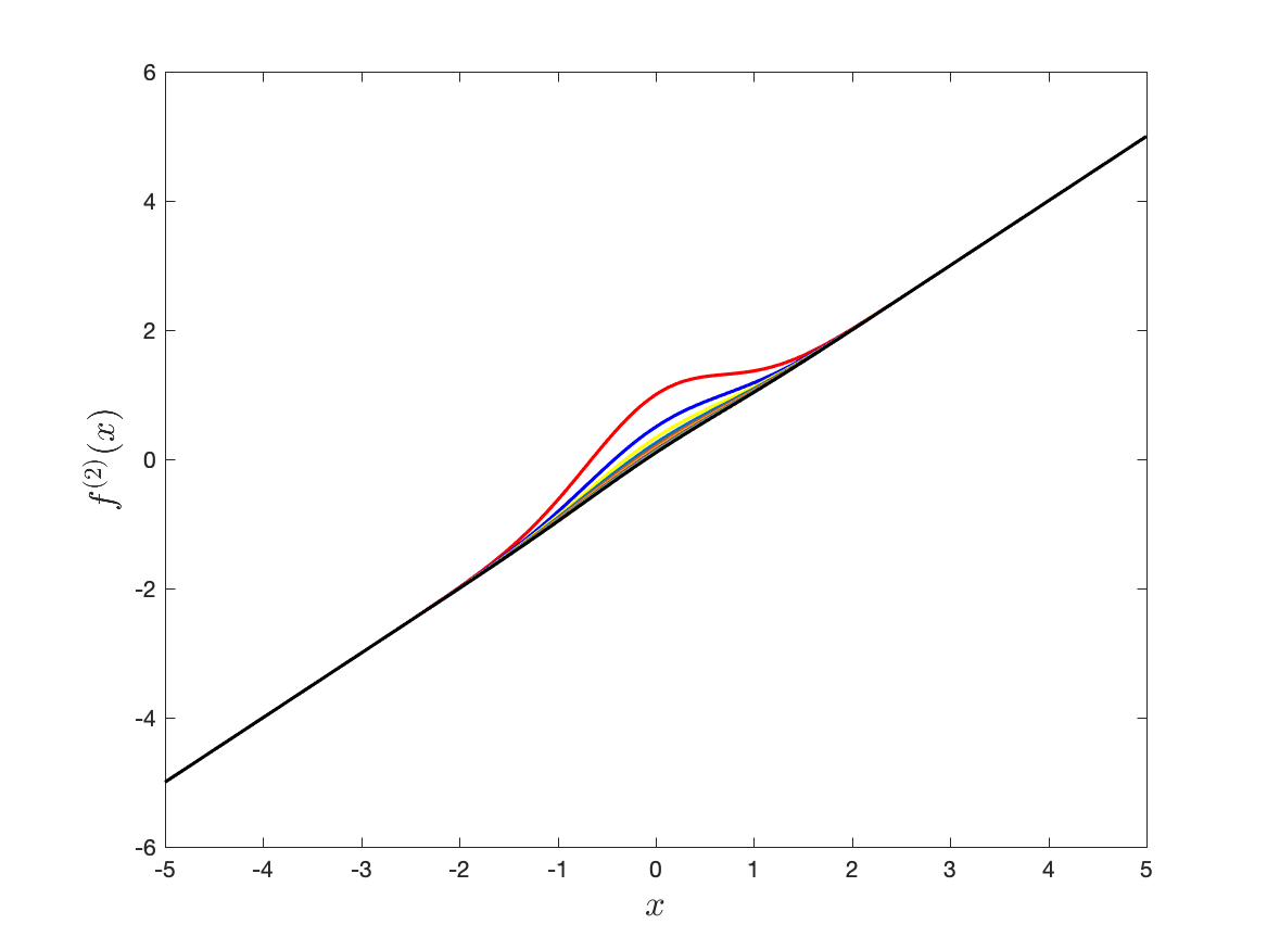
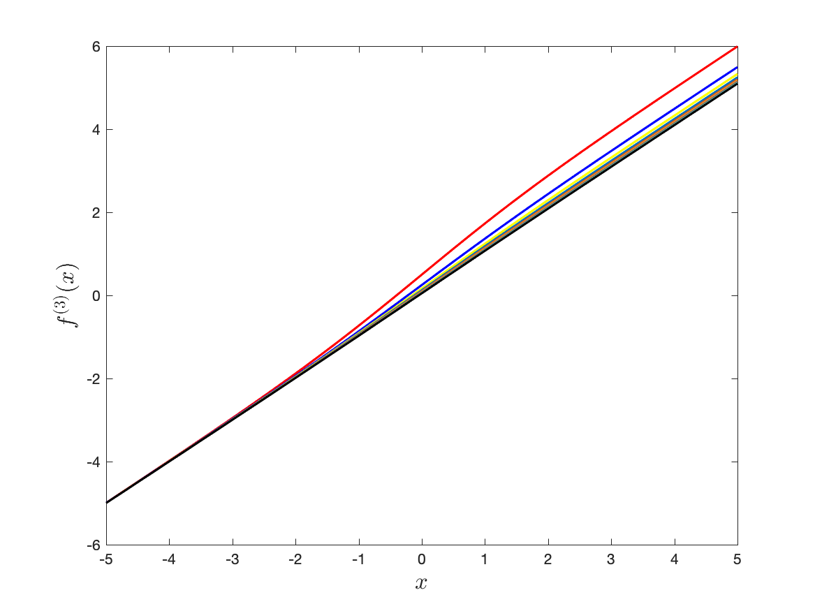
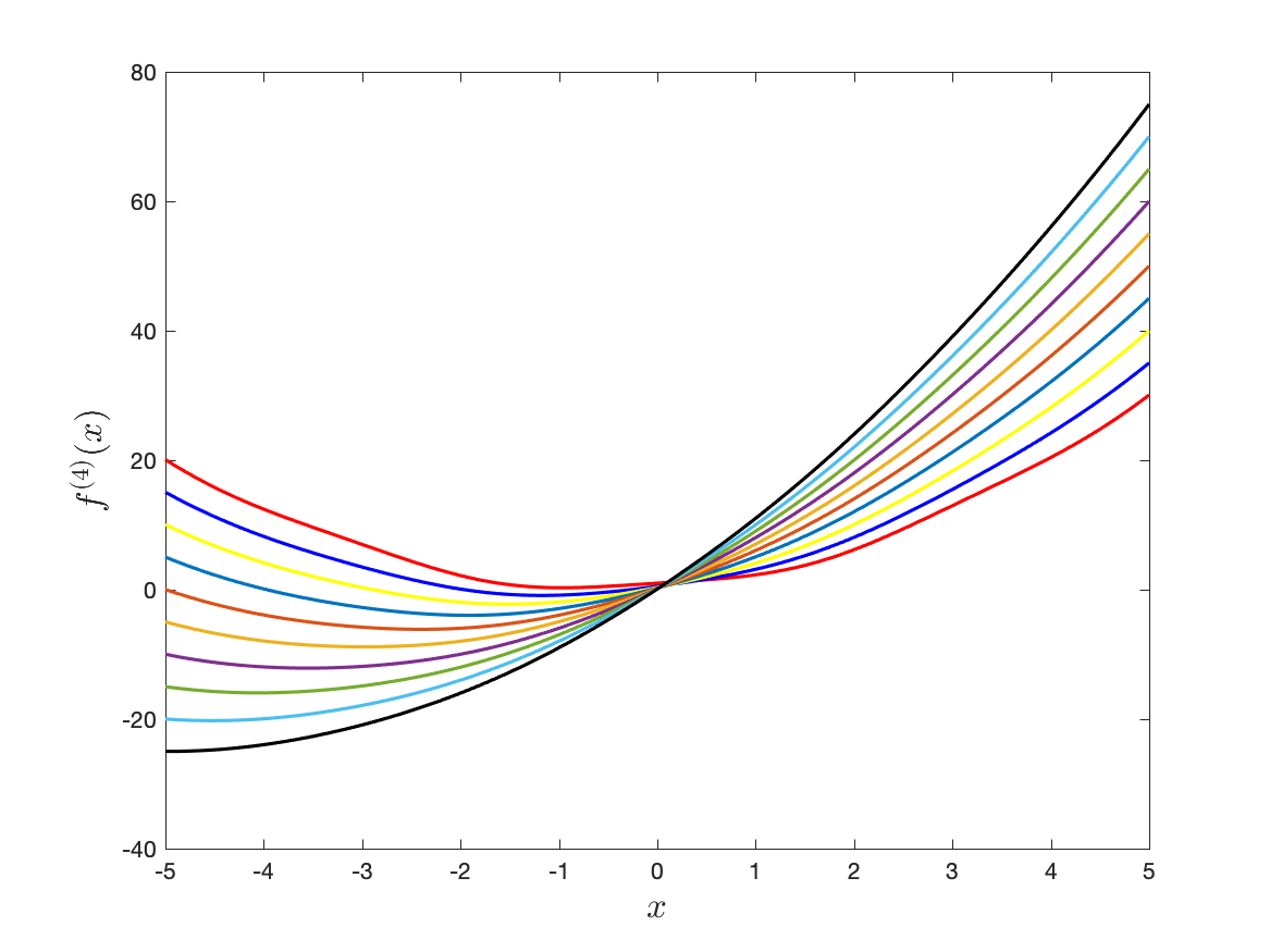
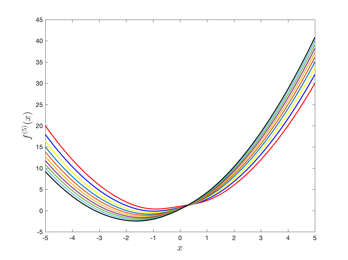
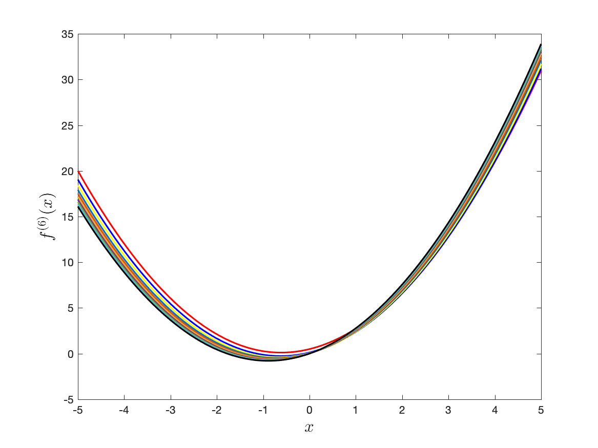
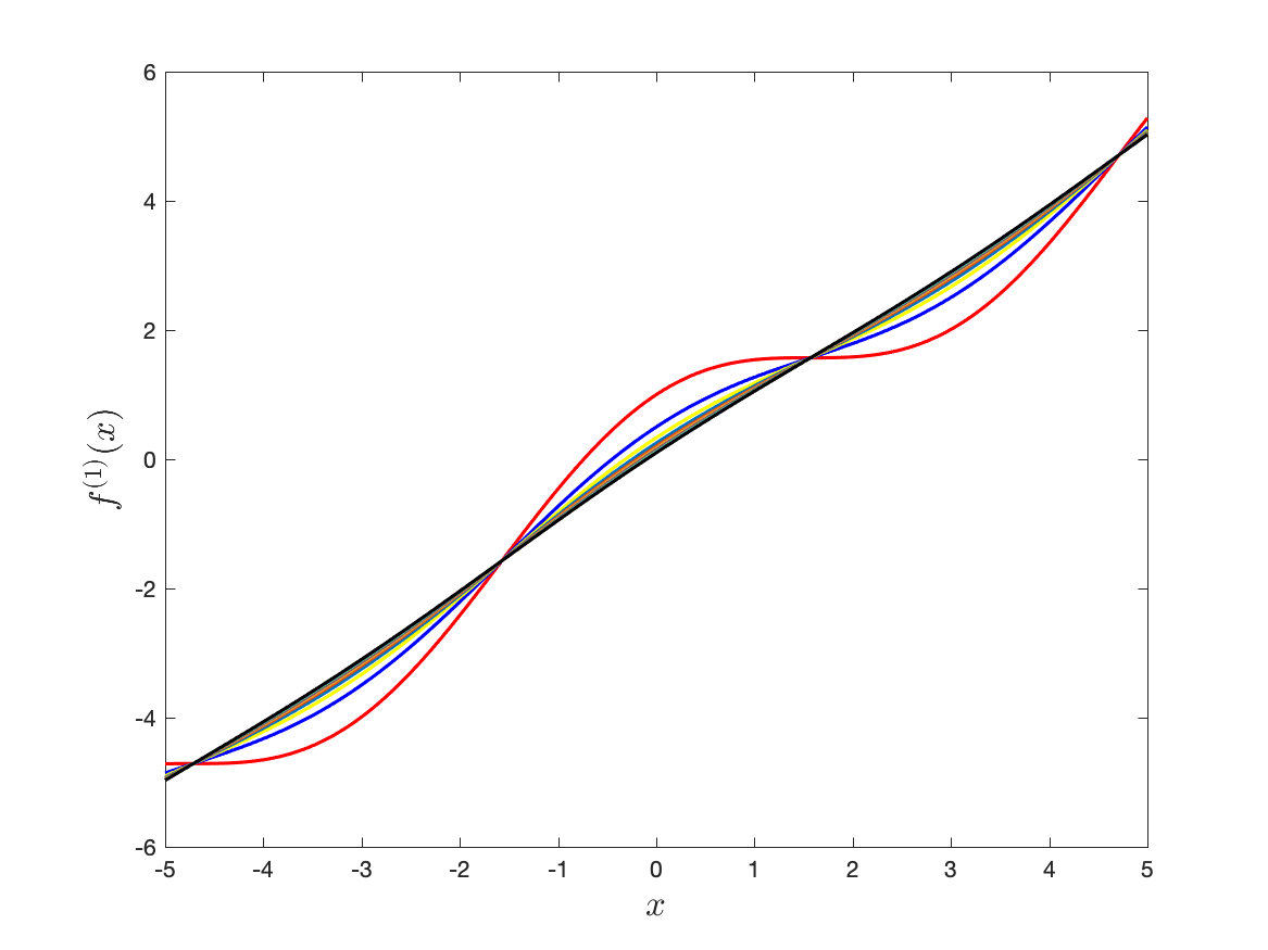
Figure 1: The link functions used in simulations. When kk varies from 11 to 1010, the line moves from red to black. The link functions in the first row are essentially linear functions combined with different fluctuations, while in the second row they are quadratic. As kk increases, the fluctuation is more and more moderate.

In this section, we illustrate the performance of our proposed estimators in different simulation settings and carry out a real data application in the end. In simulation studies, the link function is set to one of the following six forms:

fk(1)​(x)=\displaystyle f^{(1)}_{k}(x)= x+1kcos(x); fk(2)(x)=x+1kexp(−x2); fk(3)(x)=x+1kexp⁡(x)1+exp⁡(x);\displaystyle x+\frac{1}{k}\cos(x);\text{\ \ \ \ \ \ \ \ \ \ \ }f^{(2)}_{k}(x)=x+\frac{1}{k}\exp(-x^{2});\text{\ \ \ \ \ }f^{(3)}_{k}(x)=x+\frac{1}{k}\frac{\exp(x)}{1+\exp(x)};
fk(4)​(x)=\displaystyle f^{(4)}_{k}(x)= x2+kx+1kcos2(x); fk(5)(x)=x2+kx+1kexp(−x2);\displaystyle x^{2}+kx+\frac{1}{k}\cos^{2}(x);\text{\ \ }f^{(5)}_{k}(x)=x^{2}+\sqrt{k}x+\frac{1}{\sqrt{k}}\exp(-x^{2});
fk(6)​(x)=\displaystyle f^{(6)}_{k}(x)= x2+k14​x+1k2​exp⁡(x)1+exp⁡(x).\displaystyle x^{2}+k^{\frac{1}{4}}x+\frac{1}{k^{2}}\frac{\exp(x)}{1+\exp(x)}.\text{\ \ \ }

Their plots are shown in Figure 1. For all simulations we let ϵ∼N⁡(0,0.01)\epsilon\sim N(0,0.01). To measure the estimation accuracy we use the cosine distance defined by cos⁡(𝜷^,𝜷⋆)=1−|𝜷^T​𝜷⋆|/‖𝜷^‖2\cos(\hat{\bm{\beta}},\bm{\beta}^{\star})=1-|\hat{\bm{\beta}}^{T}\bm{\beta}^{\star}|/\|\hat{\bm{\beta}}\|_{2}. Note that we do not normalize 𝜷^\hat{\bm{\beta}} and change its direction according to the sign of its first entry because cosine distance is more suitable for verifying our matrix results and it allows us to generate 𝜷⋆\bm{\beta}^{\star} without restricting the first entry to be positive. We can easily see cos⁡(𝜷^k,𝜷k⋆)≍‖𝜷^k−𝜷~k‖22\cos(\hat{\bm{\beta}}_{k},\bm{\beta}^{\star}_{k})\asymp\|\hat{\bm{\beta}}_{k}-\tilde{\bm{\beta}}_{k}\|^{2}_{2}, ∀k∈[d2]\forall k\in[d_{2}]. For a matrix estimator, we will sum up cosine distance over all columns, which is a rough surrogate of ‖𝑩^−𝑩~‖F2\|\hat{\bm{B}}-\tilde{\bm{B}}\|_{F}^{2}. Our results are averaged of 40 independent runs.

7.1 Single Sparse Vector

We set d1=100d_{1}=100, d2=20d_{2}=20, s=10s=10, and vary nn only. For i∈[n]i\in[n] and k∈[d2]k\in[d_{2}], we let 𝑿i\bm{X}_{i} be independent and identically generated from one of distributions listed in Table 2, and Zi​k∈{−1,1}Z_{ik}\in\{-1,1\} with equal probability and independent from other coordinates. To generate d1d_{1}-dimensional parameter 𝜷k⋆\bm{\beta}^{\star}_{k}, we first generate the support of nonzero coefficients SkS_{k} uniformly at random and then let {[𝜷k⋆]l}l∈Sk∼i​i​d1s⋅Unif⁡({−1,1})\{[\bm{\beta}^{\star}_{k}]_{l}\}_{l\in S_{k}}\stackrel{{\scriptstyle iid}}{{\sim}}\frac{1}{\sqrt{s}}\cdot{\rm Unif}(\{-1,1\}). According to Theorem 3 and 7, we set λk=30​log⁡d1​d2/n\lambda_{k}=30\sqrt{\log d_{1}d_{2}/n} and τ=2​(n/log⁡d1​d2)1/6\tau=2(n/\log d_{1}d_{2})^{1/6}.

Distribution parameter score function
Gaussian μ=0\mu=0; σ=1\sigma=1 s⁡(x)=xs(x)=x
Beta α=8\alpha=8; β=8\beta=8 s⁡(x)=14​x−7(1−x)​xs(x)=\frac{14x-7}{(1-x)x}
Gamma k=8k=8; θ=0.1\theta=0.1 s⁡(x)=10−7xs(x)=10-\frac{7}{x}
Student’s t ν=13\nu=13 s⁡(x)=14​x13+x2s(x)=\frac{14x}{13+x^{2}}
Rayleigh σ=1\sigma=1 s⁡(x)=x−1xs(x)=x-\frac{1}{x}
Weibull k=7k=7; λ=1\lambda=1 s⁡(x)=7​x6−6xs(x)=7x^{6}-\frac{6}{x}
Table 2: Distribution of 𝐱{\bm{x}}

Figure 2 illustrates the error trend for estimating 𝜷1⋆\bm{\beta}^{\star}_{1}, 𝜷d2/2⋆\bm{\beta}^{\star}_{d_{2}/2} and 𝜷d2⋆\bm{\beta}^{\star}_{d_{2}} under different link functions and 𝒙{\bm{x}} following one of the following distributions: Gaussian, Beta or Gamma. Additional results are shown in Figure 9 in Appendix D for 𝒙{\bm{x}} following t13t_{13}, Rayleigh or Weibull distributions. From the plots, we see the error for using linear link functions (f(1)f^{(1)} to f(3)f^{(3)}) is generally smaller than the error for using quadratic link functions (f(4)f^{(4)} to f(6)f^{(6)}), no matter which distribution we use for design. But in all settings the scaled error plots have a linear trend when n≫s​log⁡d1​d2n\gg s\log d_{1}d_{2}, which is consistent with Theorem 7. Another interesting observation is that, as kk increases, the estimation will be more and more precise. This can also be seen from our theoretical results. Note that quadratic function f⁡(x)=x2f(x)=x^{2} brings the singularity to the estimation problem even for the Gaussian design since 𝔼⁡[f′​(⟨𝒙,𝜷⋆⟩)]=0\mathbb{E}[f^{\prime}(\langle{\bm{x}},\bm{\beta}^{\star}\rangle)]=0. Thus, when kk is small, the scalar μk\mu_{k}, appeared in (5), will be close to zero, which implies that the estimation problem is almost singular. Fortunately, when kk is large, the linear term in quadratic functions will have more contributions and μk≈k\mu_{k}\approx k. From Corollary 5 and identity (5), we see that μk\mu_{k} amplifies the magnitude of the signal 𝜷k⋆\bm{\beta}^{\star}_{k} that characterizes the difficulty of estimation problem. Therefore a larger μk\mu_{k} implies an easier problem. Figure 10—12 in Appendix D provide additional simulation results where we plot the error trend for all d2d_{2} parameters, which make this observation more clear.

Refer to caption
(a) Gaussian for 𝜷1⋆\bm{\beta}^{\star}_{1}
Refer to caption
(b) Gaussian for 𝜷d2/2⋆\bm{\beta}^{\star}_{d_{2}/2}
Refer to caption
(c) Gaussian for 𝜷d2⋆\bm{\beta}^{\star}_{d_{2}}
Refer to caption
(d) Beta for 𝜷1⋆\bm{\beta}^{\star}_{1}
Refer to caption
(e) Beta for 𝜷d2/2⋆\bm{\beta}^{\star}_{d_{2}/2}
Refer to caption
(f) Beta for 𝜷d2⋆\bm{\beta}^{\star}_{d_{2}}
Refer to caption
(g) Gamma for 𝜷1⋆\bm{\beta}^{\star}_{1}
Refer to caption
(h) Gamma for 𝜷d2/2⋆\bm{\beta}^{\star}_{d_{2}/2}
Refer to caption
(i) Gamma for 𝜷d2⋆\bm{\beta}^{\star}_{d_{2}}
Refer to caption
Figure 2: Sparse vector estimation plot (I). This figure shows cosine distance trend for error of estimating single sparse parameter in model (1). Six lines indicates six different types of link functions. Each row represents one type of distribution for design.

7.2 Low-rank Matrix

We study the estimation of 𝑩⋆\bm{B}^{\star} under the low-rank assumption. We let d1=d2=25d_{1}=d_{2}=25, r=5r=5. The distribution of 𝒙{\bm{x}} is set as described in Table 2. For generating 𝑩⋆\bm{B}^{\star}, we first generate two random orthogonal matrices 𝑼∈ℝd1×d1\bm{U}\in\mathbb{R}^{d_{1}\times d_{1}} and 𝑽∈ℝd2×d2\bm{V}\in\mathbb{R}^{d_{2}\times d_{2}}, then generate d1×d2d_{1}\times d_{2} diagonal matrix 𝚲\bm{\Lambda} by first sampling rr locations from [min⁡{d1,d2}][\min\{d_{1},d_{2}\}] and further setting each entry to be {−1r,1r}\{-\frac{1}{\sqrt{r}},\frac{1}{\sqrt{r}}\} with equal probability. Finally we let 𝑩⋆=𝑼​𝚲​𝑽T\bm{B}^{\star}=\bm{U}\bm{\Lambda}\bm{V}^{T}. We consider both independent and dependent 𝒛{\bm{z}}. For the independent case, 𝒛{\bm{z}} is generated as in the previous section. For the dependent case, we generate 𝒛{\bm{z}} as follows. Using the Gaussian copula with the correlation matrix 𝚺=0.2⋅𝟏d2​𝟏d2T+0.8​𝑰d2\bm{\Sigma}=0.2\cdot\boldsymbol{1}_{d_{2}}\boldsymbol{1}_{d_{2}}^{T}+0.8\boldsymbol{I}_{d_{2}}, we generate d2d_{2}-dimensional random vectors with support in [0,1]d2[0,1]^{d_{2}}. Then we apply inverse transformation on each coordinate to make it marginally distributed as t7t_{7}. Note that under our setup 𝒛{\bm{z}} has dependent coordinates with each coordinate being t7t_{7} distribution. However, the true covariance matrix of 𝒛{\bm{z}} is not 𝚺\bm{\Sigma} anymore and is even unknown. According to Theorem 9, we set κ1=2​log⁡(d1+d2)/n⁡(d1+d2)\kappa_{1}=2\sqrt{\log(d_{1}+d_{2})/n(d_{1}+d_{2})} and λ=12​(d1+d2)​log⁡(d1+d2)/n\lambda=12\sqrt{(d_{1}+d_{2})\log(d_{1}+d_{2})/n}. The precision matrix estimator we use is defined in (14) with κ2=2​log⁡d2/n​d2\kappa_{2}=2\sqrt{\log d_{2}/nd_{2}}, suggested by Lemma 12.

Figure 3 and 4 summarize our results. We observe a linear trend for all link functions, though the quadratic link functions result in a larger error overall. Also, for each distribution, dependent or independent 𝒛{\bm{z}} have very similar error trends among all six types of link functions. This observation verifies our theoretical results in Theorem 9 and Lemma 12 that estimating precision matrix only contributes higher order error.

Refer to caption
(a) Gaussian
Refer to caption
(b) Beta
Refer to caption
(c) Gamma
Refer to caption
(d) t13t_{13}
Refer to caption
(e) Rayleigh
Refer to caption
(f) Weibull
Refer to caption
Figure 3: Low-rank matrix estimation plot. This figure shows ‖𝑩^−𝑩~‖F\|\hat{\bm{B}}-\tilde{\bm{B}}\|_{F} error of estimating low-rank parameter matrix in model (1). Six lines indicates six different types of link functions. Components of 𝒛{\bm{z}} are independent.
Refer to caption
(a) Gaussian
Refer to caption
(b) Beta
Refer to caption
(c) Gamma
Refer to caption
(d) t13t_{13}
Refer to caption
(e) Rayleigh
Refer to caption
(f) Weibull
Refer to caption
Figure 4: Low-rank matrix estimation plot. This figure shows ‖𝑩^−𝑩~‖F\|\hat{\bm{B}}-\tilde{\bm{B}}\|_{F} error of estimating low-rank parameter matrix in model (1). Six lines indicates six different types of link functions. Components of 𝒛{\bm{z}} are dependent.

7.3 Sparse Matrix

For the sparse matrix recovery, we only consider estimating fully sparse 𝑩⋆\bm{B}^{\star} with dependent covariate 𝒛{\bm{z}}. We let d1=100d_{1}=100, d2=50d_{2}=50, s=10s=10. The considered distributions for design 𝒙{\bm{x}} are in Table 2. 𝑩⋆\bm{B}^{\star} is generated by first generating the support of nonzero entries and then setting each entry on the support to be {−1s,1s}\{-\frac{1}{\sqrt{s}},\frac{1}{\sqrt{s}}\} with equal probability. For generating dependent 𝒛{\bm{z}}, we define the sparse precision matrix Θ=(θi​j)i,j=1d2\Theta=(\theta_{ij})_{i,j=1}^{d_{2}} as follows

θi​j={1if ​i=j,0.2if ​|i−j|=1,0otherwise.\displaystyle\theta_{ij}=\begin{cases}1&\text{if\ }i=j,\\ 0.2&\text{if\ }|i-j|=1,\\ 0&\text{otherwise}.\end{cases}

Then we calculate the corresponding covariance matrix Θ−1\Theta^{-1} and convert it to correlation matrix. Following the same steps as in the previous section, we use Gaussian copula to derive dependent covariates 𝒛{\bm{z}}, whose marginal distribution for each coordinate is t7t_{7}. The precision matrix of 𝒛{\bm{z}} has the same sparsity structure as Θ\Theta, even though it is not equal to Θ\Theta. According to Theorem 13, we set τ=2​(n/log⁡d1​d2)1/6\tau=2(n/\log d_{1}d_{2})^{1/6} and λ=10​log⁡d1​d2/n\lambda=10\sqrt{\log d_{1}d_{2}/n}. The sparse precision matrix estimator is defined in (A.1) and (A.2) with truncation threshold 2​(n/log⁡d2)1/42(n/\log d_{2})^{1/4} and γ=10​log⁡d2/n\gamma=10\sqrt{\log d_{2}/n}. We use default settings in CVX package (Grant and Boyd 2008; Grant and Boyd 2012) to solve (A.1) efficiently. The error plot is shown in Figure 5 and linear trends for errors appear again, as explained by Theorem 13.

Refer to caption
(a) Gaussian
Refer to caption
(b) Beta
Refer to caption
(c) Gamma
Refer to caption
(d) t13t_{13}
Refer to caption
(e) Rayleigh
Refer to caption
(f) Weibull
Refer to caption
Figure 5: Sparse matrix estimation plot. This figure shows ‖𝑩^−𝑩~‖F\|\hat{\bm{B}}-\tilde{\bm{B}}\|_{F} error of estimating sparse parameter matrix in model (1) with dependent 𝒛{\bm{z}}. Six lines indicates six different types of link functions. All above simulation results are consistent with Theorem 13.

7.4 Real Data Application

In this subsection, we will further illustrate the proposed method by analyzing a Coffea canephora genetic data set.33 3 The data set was obtained from Dryad at https://datadryad.org/resource/doi:10.5061/dryad.1139fm7. The data set collects three important traits (phenotypes): production of coffee beans (y1)(y_{1}), leaf rust incidence (y2)(y_{2}) and yield of green beans (y3)(y_{3}), from two recurrent selection populations (x1)(x_{1}) of Coffea canephora and each one of traits is evaluated at two locations (x2)(x_{2}). For each individual sample, the single nucleotide polymorphisms (SNPs)—genotype {zj}\{z_{j}\}—are identified by Genotyping-by-Sequencing. In particular, the population group (x1)(x_{1}) and the evaluation location (x2)(x_{2}) are two confounders which may modify the effect of each SNP (zj)(z_{j}) on traits (y1,y2,y3)(y_{1},y_{2},y_{3}). To study this higher-level effect from confounders, we consider the varying index coefficient model in (1), which in this case is written as

yi=∑j=1d2zj⋅fj((βj1,i)⋆x1+(βj2,i)⋆x2)+ϵ, ∀i=1,2,3,\displaystyle y_{i}=\sum_{j=1}^{d_{2}}z_{j}\cdot f_{j}\big((\beta_{j}^{1,i})^{\star}x_{1}+(\beta_{j}^{2,i})^{\star}x_{2}\big)+\epsilon,\text{\ \ \ }\forall i=1,2,3, (17)

and focus on estimating parameter matrices 𝑩i⋆=((𝜷1,i)⋆,(𝜷2,i)⋆)T∈ℝ2×d2\bm{B}^{\star}_{i}=\big((\bm{\beta}^{1,i})^{\star},(\bm{\beta}^{2,i})^{\star}\big)^{T}\in\mathbb{R}^{2\times d_{2}}.

We follow the preprocessing steps described in Ferrão et al. 2018. The data set has n=215n=215 samples evaluated at two locations in total, where n1=119n_{1}=119 of them are collected from the first population group with 4574845748 SNPs measured, while n2=96n_{2}=96 of them are collected from the second population group with 5933259332 SNPs measured. There are 3810638106 SNPs in common and we select d2=250d_{2}=250 from them uniformly at random. To make individuals independent from each other, in each group we only use the data evaluated at the first location for the first half of individuals and the data evaluated at the second location for the second half of individuals. Continuous distributions are used for the confounders x1x_{1} and x2x_{2}. In particular, we let x1∼N⁡(0,1)x_{1}\sim N(0,1), if the observation is from the first population group and x1∼N⁡(50,1)x_{1}\sim N(50,1), if it is from the second population group. Analogously, we have x2∼t13x_{2}\sim t_{13}, if the observation is evaluated at the first location and x2∼50+t13x_{2}\sim 50+t_{13}, if it is evaluated at the second location. Here t13t_{13} refers to the tt distribution with degree of freedom 1313. Under our setup, the confounders come from the following mixture distribution:

x1∼n1nN(0,1)+n2nN(50,1), x2∼12t13+12(50+t13).\displaystyle x_{1}\sim\frac{n_{1}}{n}N(0,1)+\frac{n_{2}}{n}N(50,1),\text{\ \ \ }x_{2}\sim\frac{1}{2}t_{13}+\frac{1}{2}(50+t_{13}). (18)

The corresponding score functions are computed based on the above distributions. We note that the data set is a high-dimensional one, since n<d2n<d_{2}, and 𝑩i⋆\bm{B}^{\star}_{i} cannot be estimated using many of the related works, where typically d2<5d_{2}<5 (Huang and Zhang 2013; Guo et al. 2016; Zhao et al. 2017). The histograms for three traits are provided in Figure 6. Note that they have been normalized as in Ferrão et al. 2018. We also refer to Ferrão et al. 2018 for other basic statistical analysis and detailed preprocessing steps on this data set.

Refer to caption
(a) Production
Refer to caption
(b) Leaf rust
Refer to caption
(c) Green beans
Figure 6: Histograms for three traits: production of coffee beans, leaf rust incidence and yield of green beans.
Refer to caption
(a) Production
Refer to caption
(b) Leaf rust
Refer to caption
(c) Green beans
Refer to caption
(d) Production
Refer to caption
(e) Leaf rust
Refer to caption
(f) Green beans
Figure 7: Signal trajectories. Each plot corresponds to a pair of confounders and responses, i.e. (l,i)(l,i) plot shows the trajectory of (𝜷l,i)⋆(\bm{\beta}^{l,i})^{\star} where l=1,2l=1,2 indexes the confounder and i=1,2,3i=1,2,3 indexes the response.
Refer to caption
(a) Production
Refer to caption
(b) Leaf rust
Refer to caption
(c) Green beans
Refer to caption
(d) Production
Refer to caption
(e) Leaf rust
Refer to caption
(f) Green beans
Figure 8: Signal trajectories for 95%95\% confidence interval (nonparametric bootstrapping). The (l,i)(l,i) plot shows the confidence interval trajectory of (𝜷l,i)⋆(\bm{\beta}^{l,i})^{\star} where l=1,2l=1,2 indexes the confounder and i=1,2,3i=1,2,3 indexes the response. The blue line indicates the upper bound, the red line indicates the estimator, and the green line indicates the lower bound.

For each i=1,2,3i=1,2,3, we assume that 𝑩i⋆\bm{B}^{\star}_{i} is fully sparse. We compute the sparse matrix estimator via (16)(\ref{equ:13}) with τ=(n/log⁡d1​d2)6\tau=\big(n/\log d_{1}d_{2}\big)^{6} and λ=log⁡d1​d2/n\lambda=\sqrt{\log d_{1}d_{2}/n}. The sparse precision matrix is estimated by conducting CLIME procedure with γ=5​log⁡d2/n\gamma=5\sqrt{\log d_{2}/n}. Throughout the experiment, we apply the hard truncation on confounders only since other variables are light-tailed already (for example, SNPs take value in {−1,0,1}\{-1,0,1\}). The estimated signal trajectories are drawn in Figure 7. From the plots, we observe that when fitting y1y_{1} under the model (17), both confounders may cause different effect sizes for 55 out of 250250 selected SNPs, and 33 of them affect common SNPs. However, confounders have no effects on selected SNPs when fitting y2y_{2}, while have dense effects when fitting y3y_{3}. In the latter case, we should mention the signals with large magnitude are still sparse.

In addition, we provide the 95%95\% confidence interval for each trajectory using a nonparametric bootstrap: we sample the data set with replacement for 100100 times and for each data set we estimate 𝑩i⋆\bm{B}^{\star}_{i} using the same method with the same parameters, then compute 0.0250.025 and 0.9750.975 quantiles to construct the confidence interval. The results are shown in Figure 8 where the width of confidence interval indicates the variance of our estimators. We see some of identified signals have large variance but all unidentified signals have small variance. As a complement of analysis, we also conduct parametric bootstrapping: we generate new confounders x1x_{1}, x2x_{2} from distribution in (18) for 1000010000 times, and for each new data set we estimate 𝑩i⋆\bm{B}^{\star}_{i} with the same setup, then use quantiles to construct confidence interval. The plots for parametric bootstrapping are provided in Figure 13 in Appendix D and similar observations appear again. Our code is available for download at: https://github.com/senna1128/Varying-Index-Coefficient-Models.

8 Conclusion

In this paper, we proposed new estimators based on Stein’s identity for varying index coefficient models. By utilizing score function, we can either estimate a single sparse vector or a low-rank/sparse parameter matrix. The estimator can handle dependent covariates 𝒛{\bm{z}} through estimation of the precision matrix and can achieve optimal convergence rate in sparse estimation and near optimal rate in low-rank estimation. In all cases, the estimators we proposed have closed form and are easy to implement. Instead of assuming that covariates 𝒙{\bm{x}} follow an elliptical distribution, we only require certain finite moment assumption on response yy, covariates 𝒛{\bm{z}}, and score variable S⁡(𝒙)S({\bm{x}}). We also conduct extensive numerical experiments to illustrate our result.

There are still many open problems worth exploring. One of future work is about finite moment assumption. Under the general sparsity assumption, we believe that finite 66-th moment condition is mild enough, however whether it is possible to relax it further is not clear. Furthermore, we note that all first-order Stein’s estimators suffer from μk=𝔼⁡[fk′​(⟨𝒙,𝜷k⋆⟩)]=0\mu_{k}=\mathbb{E}[f_{k}^{\prime}(\langle{\bm{x}},\bm{\beta}^{\star}_{k}\rangle)]=0. Therefore developing a second-order Stein’s estimator is of practical interest and will be explored elsewhere.

acknowledgments-disclosure-of-funding.
This work was completed in part with resources provided by the University of Chicago Research Computing Center. We thank Kenji Fukumizu and two anonymous reviewers for helpful comments.

Appendix A Estimate of Sparse Precision Matrix

We propose an approach to estimate a high-dimensional sparse precision matrix for heavy-tailed variable. Suppose 𝒛{\bm{z}} has finite 44th moment and 𝛀⋆=(𝚺⋆)−1\bm{\Omega}^{\star}=(\bm{\Sigma}^{\star})^{-1}, with 𝚺⋆=𝔼⁡[𝒛​𝒛T]\bm{\Sigma}^{\star}=\mathbb{E}[{\bm{z}}{\bm{z}}^{T}], is column sparse. In particular, we assume that 𝛀⋆∈ℱwK\bm{\Omega}^{\star}\in\mathcal{F}_{w}^{K}44 4 See definition in Section 5. for some ww and KK. In this setting, we estimate the precision matrix using the CLIME procedure (Cai et al. 2011)

min\displaystyle\min ‖𝛀‖1,1,\displaystyle\|\bm{\Omega}\|_{1,1}, (A.1)
s.t.\displaystyle\text{s.t.} ‖𝚺^​𝛀−𝑰d2‖max≤γ\displaystyle\|\hat{\bm{\Sigma}}\bm{\Omega}-\bm{I}_{d_{2}}\|_{\max}\leq\gamma

but with

𝚺^=1n​∑i=1n𝒁iˇ​𝒁iˇT\displaystyle\hat{\bm{\Sigma}}=\frac{1}{n}\sum_{i=1}^{n}\widecheck{\bm{Z}_{i}}\widecheck{\bm{Z}_{i}}^{T} (A.2)

being a thresholded estimator of the covariance matrix for some threshold τ>0\tau>0, and γ\gamma is a tuning parameter. The linear program in (A.1) is the same as in Cai et al. 2011, with the difference that we use an estimator of 𝚺⋆\bm{\Sigma}^{\star} that is more suitable for heavy-tailed data.

Lemma 15.

If τ=(M4​n/log⁡d2)1/4/2\tau=(M_{4}n/\log d_{2})^{1/4}/2 and γ=12​‖𝛀⋆‖1​M4​log⁡d2/n\gamma=12\|\bm{\Omega}^{\star}\|_{1}\sqrt{M_{4}\log d_{2}/n}, the estimator (A.1) satisfies

P⁡(‖𝛀^−𝛀⋆‖2≤96​‖𝛀⋆‖12​w​M4​log⁡d2/n)≥1−2d22,\displaystyle P\bigg(\|\hat{\bm{\Omega}}-\bm{\Omega}^{\star}\|_{2}\leq 96\|\bm{\Omega}^{\star}\|_{1}^{2}w\sqrt{M_{4}\log d_{2}/n}\bigg)\geq 1-\frac{2}{d_{2}^{2}},

and

P⁡(‖𝛀^−𝛀⋆‖max≤48​‖𝛀⋆‖12​M4​log⁡d2/n)≥1−2d22.\displaystyle P\bigg(\|\hat{\bm{\Omega}}-\bm{\Omega}^{\star}\|_{\max}\leq 48\|\bm{\Omega}^{\star}\|_{1}^{2}\sqrt{M_{4}\log d_{2}/n}\bigg)\geq 1-\frac{2}{d_{2}^{2}}.

From above lemma, we see the setting for γ\gamma in (A.1) is oracle in the sense that ‖𝛀⋆‖1\|\bm{\Omega}^{\star}\|_{1} is unknown. Cai et al. 2011 showed a detailed discussion on this aspect and this dependence could be removed by using a self-calibrated estimator, similar to scaled lasso (Sun and Zhang 2013). We should also mention that (A.1) achieves the optimal rate (Cai et al. 2016).

Appendix B Proofs of Lemmas

Throughout the proof, we frequently utilize the Bernstein’s inequality presented in Corollary 2.11 in Boucheron et al. 2013. To simplify subsequent presentation, we define a function to denote the common upper bound:

φ⁡(t,a,b)=exp⁡(−t2/2a+b⋅t/3).\displaystyle\varphi(t,a,b)=\exp(-\frac{t^{2}/2}{a+b\cdot t/3}).

As shown in Bernstein’s inequality, usually aa measures the total variance and bb is bound for a single variable. We also use MM as the substitute of MpM_{p} (pp is certain moment) for simplicity. We summarize all structures we used in the paper for future reference.

Assumption 16 (Column-wise sparse).

We assume ‖𝛃k⋆‖0≤s\|\bm{\beta}^{\star}_{k}\|_{0}\leq s, ∀k∈[d2]\forall k\in[d_{2}].

Assumption 17 (Fully sparse).

We assume 𝐁⋆\bm{B}^{\star} is ss-sparse: ‖𝐁⋆‖0,1=|supp​(𝐁⋆)|≤s\|\bm{B}^{\star}\|_{0,1}=|\text{supp}(\bm{B}^{\star})|\leq s.

Assumption 18 (Low-rank).

We assume 𝐁⋆\bm{B}^{\star} satisfies rank​(𝐁⋆)≤r\text{rank}(\bm{B}^{\star})\leq r.

Assumption 19 (Independence).

We assume 𝐳{\bm{z}} satisfies 𝔼⁡[zi​zj]=0\mathbb{E}[z_{i}z_{j}]=0, ∀i≠j∈[d2]\forall i\neq j\in[d_{2}].

Assumption 20 (Precision matrix restriction).

Define 𝚺⋆=𝔼⁡[𝐳​𝐳T]\bm{\Sigma}^{\star}=\mathbb{E}[{\bm{z}}{\bm{z}}^{T}] and let 𝛀⋆=(𝚺⋆)−1\bm{\Omega}^{\star}=(\bm{\Sigma}^{\star})^{-1}, we assume

𝛀⋆∈ℱwK={𝛀∈ℝd2×d2:∥𝛀∥0,∞≤w,∥𝛀∥2≤K,∥𝛀−1∥2≤K}\displaystyle\bm{\Omega}^{\star}\in\mathcal{F}_{w}^{K}=\bigg\{\bm{\Omega}\in\mathbb{R}^{d_{2}\times d_{2}}:\|\bm{\Omega}\|_{0,\infty}\leq w,\|\bm{\Omega}\|_{2}\leq K,\|\bm{\Omega}^{-1}\|_{2}\leq K\bigg\}

for some ww and KK.

B.1 Proof of Lemma 4

Under Assumption 2, we can get from (7) that

∇L^k​(𝜷~k)=2​𝜷~k−2n​∑i=1nyi​Zi​k​𝑿i=(5)2​(𝔼⁡[y​zk⋅𝒙]−1n​∑i=1nyi​Zi​k​𝑿i).\displaystyle\nabla\hat{L}_{k}(\tilde{\bm{\beta}}_{k})=2\tilde{\bm{\beta}}_{k}-\frac{2}{n}\sum_{i=1}^{n}y_{i}Z_{ik}\bm{X}_{i}\stackrel{{\scriptstyle(\ref{equ:3})}}{{=}}2(\mathbb{E}[yz_{k}\cdot{\bm{x}}]-\frac{1}{n}\sum_{i=1}^{n}y_{i}Z_{ik}\bm{X}_{i}).

So, for any fixed j∈[d1]j\in[d_{1}], we have

[∇L^k​(𝜷~k)]j=2​(𝔼⁡[y​zk⋅xj]−1n​∑i=1nyi​Zi​k​Xi​j).\displaystyle[\nabla\hat{L}_{k}(\tilde{\bm{\beta}}_{k})]_{j}=2(\mathbb{E}[yz_{k}\cdot x_{j}]-\frac{1}{n}\sum_{i=1}^{n}y_{i}Z_{ik}X_{ij}). (B.1)

Note that zk​xjz_{k}x_{j} is a sub-exponential random variable with

‖zk​xj‖ψ1≤‖zk‖ψ2​‖xj‖ψ2≤Υ𝒛​Υ𝒙,\displaystyle\|z_{k}x_{j}\|_{\psi_{1}}\leq\|z_{k}\|_{\psi_{2}}\|x_{j}\|_{\psi_{2}}\leq\Upsilon_{{\bm{z}}}\Upsilon_{{\bm{x}}}, (B.2)

where Υ𝒙\Upsilon_{{\bm{x}}} is ψ2\psi_{2}-norm of a standard Gaussian variable. So we see {yi,Zi​k​Xi​j}i∈[n]\{y_{i},Z_{ik}X_{ij}\}_{i\in[n]} are nn independent copies of yy and zk​xjz_{k}x_{j}. Based on Lemma C.4 in Yang et al. 2019 and (B.2), let γ=max⁡(Υy,Υ𝒙​Υ𝒛)\gamma=\max(\Upsilon_{y},\Upsilon_{{\bm{x}}}\Upsilon_{{\bm{z}}}) and we get

P⁡(|1n​∑i=1nyi​Zi​k​Xi​j−𝔼⁡[y​zk⋅xj]|>Υγ​log⁡nn)<1n2\displaystyle P(|\frac{1}{n}\sum_{i=1}^{n}y_{i}Z_{ik}X_{ij}-\mathbb{E}[yz_{k}\cdot x_{j}]|>\Upsilon_{\gamma}\sqrt{\frac{\log n}{n}})<\frac{1}{n^{2}}

where Υγ>0\Upsilon_{\gamma}>0 only depends on γ\gamma. According to equation (B.1), we can take union bound and further have

P⁡(‖∇L^k​(𝜷~k)‖∞>2​Υγ​log⁡nn)<d1n2,\displaystyle P(\|\nabla\hat{L}_{k}(\tilde{\bm{\beta}}_{k})\|_{\infty}>2\Upsilon_{\gamma}\sqrt{\frac{\log n}{n}})<\frac{d_{1}}{n^{2}},

which concludes the proof.

B.2 Proof of Lemma 8

Based on equation (8), we know

∇L¯k​(𝜷~k)=2​𝜷~k−2n​∑i=1nyiˇ​Zi​kˇ​S⁡(𝑿i)ˇ.\displaystyle\nabla\bar{L}_{k}(\tilde{\bm{\beta}}_{k})=2\tilde{\bm{\beta}}_{k}-\frac{2}{n}\sum_{i=1}^{n}\widecheck{y_{i}}\widecheck{Z_{ik}}\widecheck{S(\bm{X}_{i})}.

Under Assumption 2 and 19, we know 𝜷~k=𝔼⁡[y​zk⋅S⁡(𝒙)]\tilde{\bm{\beta}}_{k}=\mathbb{E}[yz_{k}\cdot S({\bm{x}})]. So we can separate above gradient into two parts

∥\displaystyle\| ∇L¯k(𝜷~k)∥∞=2∥𝜷~k−1n∑i=1nyˇiZi​kˇS⁡(𝑿i)ˇ∥∞\displaystyle\nabla\bar{L}_{k}(\tilde{\bm{\beta}}_{k})\|_{\infty}=2\|\tilde{\bm{\beta}}_{k}-\frac{1}{n}\sum_{i=1}^{n}\widecheck{y}_{i}\widecheck{Z_{ik}}\widecheck{S(\bm{X}_{i})}\|_{\infty}
≤\displaystyle\leq 2​‖𝔼⁡[y​zk⋅S⁡(𝒙)]−1n​∑i=1n𝔼⁡[yˇi​Zi​kˇ​S⁡(𝑿i)ˇ]⏟ℐ1‖∞+2​‖1n​∑i=1n𝔼⁡[yˇi​Zi​kˇ​S⁡(𝑿i)ˇ]−1n​∑i=1nyˇi​Zi​kˇ​S⁡(𝑿i)ˇ⏟ℐ2‖∞.\displaystyle 2\|\underbrace{\mathbb{E}[yz_{k}\cdot S({\bm{x}})]-\frac{1}{n}\sum_{i=1}^{n}\mathbb{E}[\widecheck{y}_{i}\widecheck{Z_{ik}}\widecheck{S(\bm{X}_{i})}]}_{\mathcal{I}_{1}}\|_{\infty}+2\|\underbrace{\frac{1}{n}\sum_{i=1}^{n}\mathbb{E}[\widecheck{y}_{i}\widecheck{Z_{ik}}\widecheck{S(\bm{X}_{i})}]-\frac{1}{n}\sum_{i=1}^{n}\widecheck{y}_{i}\widecheck{Z_{ik}}\widecheck{S(\bm{X}_{i})}}_{\mathcal{I}_{2}}\|_{\infty}. (B.3)

We will provide a deterministic bound for ℐ1\mathcal{I}_{1} and probabilistic bound for ℐ2\mathcal{I}_{2}. Let’s deal with ℐ1\mathcal{I}_{1} first. For any j∈[d1]j\in[d_{1}], we know

ℐ1​j=\displaystyle\mathcal{I}_{1j}= 𝔼⁡[y​zk⋅S​(𝒙)j]−𝔼⁡[yˇ​zkˇ⋅S⁡(𝒙)ˇj]\displaystyle\mathbb{E}[yz_{k}\cdot S({\bm{x}})_{j}]-\mathbb{E}[\widecheck{y}\widecheck{z_{k}}\cdot\widecheck{S({\bm{x}})}_{j}]
=\displaystyle= 𝔼⁡[y​zk⋅S​(𝒙)j⋅𝟏|y|>τ​ or ​|zk|>τ​ or ​|S​(𝒙)j|>τ]\displaystyle\mathbb{E}\big[yz_{k}\cdot S({\bm{x}})_{j}\cdot\boldsymbol{1}_{|y|>\tau\text{\ or\ }|z_{k}|>\tau\text{\ or\ }|S({\bm{x}})_{j}|>\tau}\big]
≤\displaystyle\leq 𝔼⁡[y2​𝒛k2​S​(𝒙)j2]⋅(P⁡(|y|>τ)+P⁡(|𝒛k|>τ)+P⁡(|S​(𝒙)j|>τ))\displaystyle\sqrt{\mathbb{E}[y^{2}{\bm{z}}_{k}^{2}S({\bm{x}})_{j}^{2}]\cdot\big(P(|y|>\tau)+P(|{\bm{z}}_{k}|>\tau)+P(|S({\bm{x}})_{j}|>\tau)\big)}
≤\displaystyle\leq 𝔼⁡[y4]​𝔼​[zk4]​𝔼​[S​(𝒙)j4]4​3​M1/2τ3\displaystyle\sqrt[4]{\mathbb{E}[y^{4}]\mathbb{E}[z_{k}^{4}]\mathbb{E}[S({\bm{x}})_{j}^{4}]}\frac{\sqrt{3}M^{1/2}}{\tau^{3}}
≤\displaystyle\leq 2​Mτ3.\displaystyle\frac{2M}{\tau^{3}}. (B.4)

Here, the third inequality is from Cauchy-Schwarz inequality; the fourth inequality is Chebyshev inequality; the last inequality is due to Assumption 6 (p=6p=6). So from (B.2), we know

‖ℐ1‖∞≤2​M/τ3.\displaystyle\|\mathcal{I}_{1}\|_{\infty}\leq 2M/\tau^{3}. (B.5)

For the ℐ2\mathcal{I}_{2} term in equation (B.2), we apply Bernstein’s inequality. We have ∀j∈[d1]\forall j\in[d_{1}],

−τ3≤yˇi​Zi​kˇ​S⁡(𝑿i)ˇj≤τ3⟹C=2​τ3,\displaystyle-\tau^{3}\leq\widecheck{y}_{i}\widecheck{Z_{ik}}\widecheck{S(\bm{X}_{i})}_{j}\leq\tau^{3}\Longrightarrow C=2\tau^{3}, (B.6)
Vn=∑i=1nVar​(yˇi​Zi​kˇ​S⁡(𝑿i)ˇj)≤∑i=1n𝔼⁡[yˇi2​Zi​kˇ2​S⁡(𝑿i)ˇj2]≤n​M.\displaystyle V_{n}=\sum_{i=1}^{n}\text{Var}(\widecheck{y}_{i}\widecheck{Z_{ik}}\widecheck{S(\bm{X}_{i})}_{j})\leq\sum_{i=1}^{n}\mathbb{E}[\widecheck{y}_{i}^{2}\widecheck{Z_{ik}}^{2}\widecheck{S(\bm{X}_{i})}_{j}^{2}]\leq nM.

Thus, based on (B.6), we have ∀t>0\forall t>0,

P⁡(|𝔼⁡[yˇ​zkˇ⋅S⁡(𝒙)ˇj]−1n​∑i=1nyˇi​Zi​kˇ​S⁡(𝑿i)ˇj|>t)≤2​φ​(n​t,n​M,2​τ3).\displaystyle P(\big|\mathbb{E}[\widecheck{y}\widecheck{z_{k}}\cdot\widecheck{S({\bm{x}})}_{j}]-\frac{1}{n}\sum_{i=1}^{n}\widecheck{y}_{i}\widecheck{Z_{ik}}\widecheck{S(\bm{X}_{i})}_{j}\big|>t)\leq 2\varphi(nt,nM,2\tau^{3}). (B.7)

Then we take union bound for (B.7) and get

P⁡(‖ℐ2‖∞>t)≤2​d1​φ​(n​t,n​M,2​τ3)\displaystyle P(\|\mathcal{I}_{2}\|_{\infty}>t)\leq 2d_{1}\varphi(nt,nM,2\tau^{3}) (B.8)

Combine (B.5) and (B.8) together, and take union bound over kk, we have ∀t,τ>0\forall t,\tau>0,

P(∥∇L¯k(𝜷~k)∥∞≤4​Mτ3+2t, ∀k∈[d2])≥1−2d1d2exp(−n​t22​M+2​τ3​t).\displaystyle P(\|\nabla\bar{L}_{k}(\tilde{\bm{\beta}}_{k})\|_{\infty}\leq\frac{4M}{\tau^{3}}+2t,\text{\ \ }\forall k\in[d_{2}])\geq 1-2d_{1}d_{2}\exp(-\frac{nt^{2}}{2M+2\tau^{3}t}). (B.9)

Suppose, for some positive constant c1,c2c_{1},c_{2}, we let

t=c1​log⁡d1​d2/n​ and ​τ=c21/3​(n/log⁡d1​d2)1/6.\displaystyle t=c_{1}\sqrt{\log d_{1}d_{2}/n}\text{\ \ and\ \ }\tau=c_{2}^{1/3}(n/\log d_{1}d_{2})^{1/6}. (B.10)

Then plug (B.10) into the right hand side of (B.9) and get

2​d1​d2​exp⁡(−n​t22​M+2​τ3​t)=2​d1​d2​exp⁡(−c12​log⁡d1​d22​M+2​c1​c2)≤2/d12​d22,\displaystyle 2d_{1}d_{2}\exp(-\frac{nt^{2}}{2M+2\tau^{3}t})=2d_{1}d_{2}\exp(-\frac{c_{1}^{2}\log d_{1}d_{2}}{2M+2c_{1}c_{2}})\leq 2/d_{1}^{2}d_{2}^{2}, (B.11)

if

c122​M+2​c1​c2≥3⟹c12−6​c1​c2−6​M≥0.\displaystyle\frac{c_{1}^{2}}{2M+2c_{1}c_{2}}\geq 3\Longrightarrow c_{1}^{2}-6c_{1}c_{2}-6M\geq 0. (B.12)

We can set c1=3​Mc_{1}=3\sqrt{M} and c2=M/8c_{2}=\sqrt{M}/8, which satisfies condition in (B.12) naturally. Further we know (B.11) holds. Plug this setting in (B.10) and (B.9) and we get

∥∇L¯k(𝜷~k)∥∞≤38M​log⁡d1​d2/n, ∀k∈[d2]\displaystyle\|\nabla\bar{L}_{k}(\tilde{\bm{\beta}}_{k})\|_{\infty}\leq 38\sqrt{M\log d_{1}d_{2}/n},\text{\ \ }\forall k\in[d_{2}] (B.13)

with probability at least 1−2/d12​d221-2/d_{1}^{2}d_{2}^{2}. This finishes the proof.

B.3 Proof of Lemma 10

Define ℐ3=1n​κ1​∑i=1nΦ⁡(κ1​yi⋅S⁡(𝑿i)​𝒁iT)−𝔼⁡[y⋅S⁡(𝒙)​𝒛T]\mathcal{I}_{3}=\frac{1}{n\kappa_{1}}\sum_{i=1}^{n}\Phi(\kappa_{1}y_{i}\cdot S(\bm{X}_{i})\bm{Z}_{i}^{T})-\mathbb{E}[y\cdot S({\bm{x}}){\bm{z}}^{T}], we will apply Corollary 3.1 in Minsker 2018. Let’s first bound the variance. Under Assumption 2, we know 𝔼⁡[S​(𝒙)j]=0,∀j∈[d1]\mathbb{E}[S({\bm{x}})_{j}]=0,\forall j\in[d_{1}]. So for any unit vector 𝒗∈ℝd1\bm{v}\in\mathbb{R}^{d_{1}}, we have

𝔼[y2\displaystyle\mathbb{E}[y^{2} ⋅𝒗TS(𝒙)𝒛T𝒛S(𝒙)T𝒗]=𝔼[y2⋅𝒛T𝒛⋅(S(𝒙)T𝒗)2]≤𝔼⁡[y4]​𝔼​[(𝒛T​𝒛)2]​𝔼​[(S​(𝒙)T​𝒗)4]\displaystyle\cdot\bm{v}^{T}S({\bm{x}}){\bm{z}}^{T}{\bm{z}}S({\bm{x}})^{T}\bm{v}]=\mathbb{E}[y^{2}\cdot{\bm{z}}^{T}{\bm{z}}\cdot(S({\bm{x}})^{T}\bm{v})^{2}]\leq\sqrt{\mathbb{E}[y^{4}]\mathbb{E}[({\bm{z}}^{T}{\bm{z}})^{2}]\mathbb{E}[(S({\bm{x}})^{T}\bm{v})^{4}]}
≤\displaystyle\leq M1/2​𝔼⁡[d2​(𝒛14+…+𝒛d24)]​𝔼⁡[∑i1=1d1∑i2=1d1S​(𝒙)i12​S​(𝒙)i22​𝒗i12​𝒗i22]\displaystyle M^{1/2}\sqrt{\mathbb{E}[d_{2}({\bm{z}}_{1}^{4}+...+{\bm{z}}_{d_{2}}^{4})]}\sqrt{\mathbb{E}[\sum_{i_{1}=1}^{d_{1}}\sum_{i_{2}=1}^{d_{1}}S({\bm{x}})^{2}_{i_{1}}S({\bm{x}})^{2}_{i_{2}}\bm{v}^{2}_{i_{1}}\bm{v}^{2}_{i_{2}}]}
≤\displaystyle\leq d2​M​∑i1=1d1∑i2=1d1𝔼⁡[S​(𝒙)i12​S​(𝒙)i22]​𝒗i12​𝒗i22≤d2​M​∑i1=1d1∑i2=1d1𝔼⁡[S​(𝒙)i14]​𝔼⁡[S​(𝒙)i24]​𝒗i12​𝒗i22\displaystyle d_{2}M\sqrt{\sum_{i_{1}=1}^{d_{1}}\sum_{i_{2}=1}^{d_{1}}\mathbb{E}[S({\bm{x}})^{2}_{i_{1}}S({\bm{x}})^{2}_{i_{2}}]\bm{v}^{2}_{i_{1}}\bm{v}^{2}_{i_{2}}}\leq d_{2}M\sqrt{\sum_{i_{1}=1}^{d_{1}}\sum_{i_{2}=1}^{d_{1}}\sqrt{\mathbb{E}[S({\bm{x}})^{4}_{i_{1}}]}\sqrt{\mathbb{E}[S({\bm{x}})^{4}_{i_{2}}]}\bm{v}^{2}_{i_{1}}\bm{v}^{2}_{i_{2}}}
≤\displaystyle\leq d2​M3/2.\displaystyle d_{2}M^{3/2}. (B.14)

The second inequality uses Cauchy-Schwarz inequality; the third inequality uses Assumption 2. From (B.3) we can get

‖𝔼⁡[y2⋅S⁡(𝒙)​𝒛T​𝒛​S​(𝒙)T]‖2≤d2​M3/2.\displaystyle\|\mathbb{E}[y^{2}\cdot S({\bm{x}}){\bm{z}}^{T}{\bm{z}}S({\bm{x}})^{T}]\|_{2}\leq d_{2}M^{3/2}. (B.15)

Follow the exactly same derivation in (B.3) we can also have

‖𝔼⁡[y2⋅𝒛​S​(𝒙)T​S​(𝒙)​𝒛T]‖2≤d1​M3/2.\displaystyle\|\mathbb{E}[y^{2}\cdot{\bm{z}}S({\bm{x}})^{T}S({\bm{x}}){\bm{z}}^{T}]\|_{2}\leq d_{1}M^{3/2}. (B.16)

Thus, combine (B.15) and (B.16) together, we have ∀t>0\forall t>0

P⁡(‖ℐ3‖2≥t)≤2​(d1+d2)​exp⁡(−n​κ1​t+n⁡(d1+d2)​M3/2​κ122).\displaystyle P(\|\mathcal{I}_{3}\|_{2}\geq t)\leq 2(d_{1}+d_{2})\exp(-n\kappa_{1}t+\frac{n(d_{1}+d_{2})M^{3/2}\kappa_{1}^{2}}{2}). (B.17)

In above tail bound (B.17), we let t=2​M3/4​2​(d1+d2)​log⁡(d1+d2)nt=2M^{3/4}\sqrt{\frac{2(d_{1}+d_{2})\log(d_{1}+d_{2})}{n}} and κ1=2​log⁡(d1+d2)n⁡(d1+d2)​M3/2\kappa_{1}=\sqrt{\frac{2\log(d_{1}+d_{2})}{n(d_{1}+d_{2})M^{3/2}}} and have

P⁡(‖ℐ3‖≤2​M3/4​2​(d1+d2)​log⁡(d1+d2)n)≥1−2(d1+d2)2.\displaystyle P\bigg(\|\mathcal{I}_{3}\|\leq 2M^{3/4}\sqrt{\frac{2(d_{1}+d_{2})\log(d_{1}+d_{2})}{n}}\bigg)\geq 1-\frac{2}{(d_{1}+d_{2})^{2}}. (B.18)

This is consistent with argument of lemma.

B.4 Proof of Lemma 12

Let’s first get concentration rate for ‖𝚺^−𝚺⋆‖2=‖1n​κ2​Φ​(κ2​Zi​ZiT)−𝔼⁡[𝒛​𝒛T]‖2\|\hat{\bm{\Sigma}}-\bm{\Sigma}^{\star}\|_{2}=\|\frac{1}{n\kappa_{2}}\Phi(\kappa_{2}Z_{i}Z_{i}^{T})-\mathbb{E}[{\bm{z}}{\bm{z}}^{T}]\|_{2}. We have ∀𝒗∈ℝd2\forall\bm{v}\in\mathbb{R}^{d_{2}} such that ‖𝒗‖2=1\|\bm{v}\|_{2}=1,

𝔼⁡[𝒗T​𝒛​𝒛T​𝒗]=𝔼⁡[(𝒗T​𝒛)2]≤𝔼⁡[‖𝒛‖22]≤d2​M.\displaystyle\mathbb{E}[\bm{v}^{T}{\bm{z}}{\bm{z}}^{T}\bm{v}]=\mathbb{E}[(\bm{v}^{T}{\bm{z}})^{2}]\leq\mathbb{E}[\|{\bm{z}}\|^{2}_{2}]\leq d_{2}\sqrt{M}.

Based on Corollary 3.1 in Minsker 2018, we know ∀t>0\forall t>0,

P⁡(‖𝚺^−𝚺⋆‖2≥t)≤2​d2​exp⁡(−n​κ2​t+n​d2​M​κ222).\displaystyle P(\|\hat{\bm{\Sigma}}-\bm{\Sigma}^{\star}\|_{2}\geq t)\leq 2d_{2}\exp(-n\kappa_{2}t+\frac{nd_{2}\sqrt{M}\kappa_{2}^{2}}{2}). (B.19)

In above (B.19), we let t=2​M1/4​2​d2​log⁡d2nt=2M^{1/4}\sqrt{\frac{2d_{2}\log d_{2}}{n}} and κ2=2​log⁡d2n​d2​M1/2\kappa_{2}=\sqrt{\frac{2\log d_{2}}{nd_{2}M^{1/2}}}, and have

P⁡(‖𝚺^−𝚺⋆‖2≤2​M1/4​2​d2​log⁡d2n)≥1−2d22.\displaystyle P\bigg(\|\hat{\bm{\Sigma}}-\bm{\Sigma}^{\star}\|_{2}\leq 2M^{1/4}\sqrt{\frac{2d_{2}\log d_{2}}{n}}\bigg)\geq 1-\frac{2}{d_{2}^{2}}. (B.20)

We use matrix perturbation analysis to give bound for 𝛀^\hat{\bm{\Omega}}. As shown in Chapter III Theorem 2.5 in Stewart and Sun 1990, when

‖𝛀⋆​(𝚺^−𝚺⋆)‖2≤‖𝛀⋆‖2​‖𝚺^−𝚺⋆‖2≤‖𝛀⋆‖2​4​M1/4​d2​log⁡d2/n≤1/2,\displaystyle\|\bm{\Omega}^{\star}(\hat{\bm{\Sigma}}-\bm{\Sigma}^{\star})\|_{2}\leq\|\bm{\Omega}^{\star}\|_{2}\|\hat{\bm{\Sigma}}-\bm{\Sigma}^{\star}\|_{2}\leq\|\bm{\Omega}^{\star}\|_{2}4M^{1/4}\sqrt{d_{2}\log d_{2}/n}\leq 1/2,

we know 𝛀^\hat{\bm{\Omega}} is perforce invertible and satisfies

‖𝛀^−𝛀⋆‖2≤2​‖𝛀⋆‖22​‖𝚺^−𝚺⋆‖2≤8​‖𝛀⋆‖22​M1/4​d2​log⁡d2/n,\displaystyle\|\hat{\bm{\Omega}}-\bm{\Omega}^{\star}\|_{2}\leq 2\|\bm{\Omega}^{\star}\|_{2}^{2}\|\hat{\bm{\Sigma}}-\bm{\Sigma}^{\star}\|_{2}\leq 8\|\bm{\Omega}^{\star}\|_{2}^{2}M^{1/4}\sqrt{d_{2}\log d_{2}/n}, (B.21)

with probability at least 1−2/d221-2/d_{2}^{2}. Therefore we finish the proof.

B.5 Proof of Lemma 14

We define ℐ7=𝔼⁡[y⋅S⁡(𝒙)​𝒛T]−1n​∑i=1nyˇi⋅S⁡(𝑿i)ˇ​𝒁iˇT\mathcal{I}_{7}=\mathbb{E}[y\cdot S({\bm{x}}){\bm{z}}^{T}]-\frac{1}{n}\sum_{i=1}^{n}\widecheck{y}_{i}\cdot\widecheck{S(\bm{X}_{i})}\widecheck{\bm{Z}_{i}}^{T}. For any j∈[d1],k∈[d2]j\in[d_{1}],k\in[d_{2}], we know

|(ℐ7)j​k|≤|1n​∑i=1nyˇi​Zi​kˇ​S⁡(𝑿i)ˇj−𝔼⁡[yˇi​Zi​kˇ​S⁡(𝑿i)ˇj]|+|1n​∑i=1n𝔼⁡[yˇi​Zi​kˇ​S⁡(𝑿i)ˇj]−𝔼⁡[y⋅zk⋅S​(𝒙)j]|.\displaystyle|(\mathcal{I}_{7})_{jk}|\leq|\frac{1}{n}\sum_{i=1}^{n}\widecheck{y}_{i}\widecheck{Z_{ik}}\widecheck{S(\bm{X}_{i})}_{j}-\mathbb{E}[\widecheck{y}_{i}\widecheck{Z_{ik}}\widecheck{S(\bm{X}_{i})}_{j}]|+|\frac{1}{n}\sum_{i=1}^{n}\mathbb{E}[\widecheck{y}_{i}\widecheck{Z_{ik}}\widecheck{S(\bm{X}_{i})}_{j}]-\mathbb{E}[y\cdot z_{k}\cdot S({\bm{x}})_{j}]|.

Use the same technique as in (B.2)-(B.8), we can get that ∀t,τ>0\forall t,\tau>0

P⁡(‖ℐ7‖max>t+2​Mτ3)≤2​d1​d2​exp⁡(−n​t22​M+2​τ3​t).\displaystyle P(\|\mathcal{I}_{7}\|_{\max}>t+\frac{2M}{\tau^{3}})\leq 2d_{1}d_{2}\exp(-\frac{nt^{2}}{2M+2\tau^{3}t}).

We let t=3​M​log⁡d1​d2/nt=3\sqrt{M\log d_{1}d_{2}/n}, τ=(M​n/log⁡d1​d2)1/6/2\tau=(Mn/\log d_{1}d_{2})^{1/6}/2 and have

P⁡(‖ℐ7‖max≤19​M​log⁡d1​d2n)≥1−2/d12​d22.\displaystyle P\bigg(\|\mathcal{I}_{7}\|_{\max}\leq 19\sqrt{\frac{M\log d_{1}d_{2}}{n}}\bigg)\geq 1-2/d_{1}^{2}d_{2}^{2}. (B.22)

So we finish the proof of lemma.

B.6 Proof of Lemma 15

We first prove a concentration bound for truncated empirical covariance 𝚺^\hat{\bm{\Sigma}}. ∀j,k∈[d2]\forall j,k\in[d_{2}],

|Σ^j​k−Σj​k⋆|=|1n​∑i=1nZi​jˇ​Zi​kˇ−𝔼⁡[zj​zk]|≤|1n​∑i=1n(Zi​jˇ​Zi​kˇ−𝔼⁡[Zi​jˇ​Zi​kˇ])|⏟ℐ5+|1n​∑i=1n𝔼⁡[Zi​jˇ​Zi​kˇ]−𝔼⁡[zj​zk]|⏟ℐ6.|\hat{\Sigma}_{jk}-\Sigma^{\star}_{jk}|=|\frac{1}{n}\sum_{i=1}^{n}\widecheck{Z_{ij}}\widecheck{Z_{ik}}-\mathbb{E}[z_{j}z_{k}]|\\ \leq\underbrace{|\frac{1}{n}\sum_{i=1}^{n}(\widecheck{Z_{ij}}\widecheck{Z_{ik}}-\mathbb{E}[\widecheck{Z_{ij}}\widecheck{Z_{ik}}])|}_{\mathcal{I}_{5}}+\underbrace{|\frac{1}{n}\sum_{i=1}^{n}\mathbb{E}[\widecheck{Z_{ij}}\widecheck{Z_{ik}}]-\mathbb{E}[z_{j}z_{k}]|}_{\mathcal{I}_{6}}. (B.23)

Use Bernstein’s inequality for ℐ5\mathcal{I}_{5}, we have

−τ2≤Zi​jˇ​Zi​kˇ≤τ2,\displaystyle-\tau^{2}\leq\widecheck{Z_{ij}}\widecheck{Z_{ik}}\leq\tau^{2},
Vn=∑i=1nVar​(Zi​jˇ​Zi​kˇ)≤∑i=1n𝔼⁡[Zi​jˇ2​Zi​kˇ2]≤n​M.\displaystyle V_{n}=\sum_{i=1}^{n}\text{Var}(\widecheck{Z_{ij}}\widecheck{Z_{ik}})\leq\sum_{i=1}^{n}\mathbb{E}[\widecheck{Z_{ij}}^{2}\widecheck{Z_{ik}}^{2}]\leq nM.

Note that the above last inequality holds no matter whether j=kj=k or not. Thus, ∀t>0\forall t>0, we have

P⁡(|ℐ5|>t)≤2​φ​(n​t,n​M,2​τ2).\displaystyle P(|\mathcal{I}_{5}|>t)\leq 2\varphi(nt,nM,2\tau^{2}). (B.24)

For the term ℐ6\mathcal{I}_{6}, we know

|ℐ6|=\displaystyle|\mathcal{I}_{6}|= 𝔼[zjzk⋅𝟏{|zj|>τ or |zk|>τ}]≤𝔼⁡[zj2​zk2]⋅(P⁡(|zj|>τ)+P⁡(|zk|>τ))≤2​Mτ2.\displaystyle\mathbb{E}[z_{j}z_{k}\cdot\boldsymbol{1}_{\{|z_{j}|>\tau\text{\ or\ }|z_{k}|>\tau\}}]\leq\sqrt{\mathbb{E}[z_{j}^{2}z_{k}^{2}]\cdot(P(|z_{j}|>\tau)+P(|z_{k}|>\tau))}\leq\frac{2M}{\tau^{2}}. (B.25)

Combine (B.23), (B.24) and (B.25) together, we get

|Σ^j​k−Σj​k⋆|≤t+2​Mτ2,\displaystyle|\hat{\Sigma}_{jk}-\Sigma^{\star}_{jk}|\leq t+\frac{2M}{\tau^{2}}, (B.26)

with probability at least 1−2​exp⁡(−n​t22​M+2​τ2​t)1-2\exp(-\frac{nt^{2}}{2M+2\tau^{2}t}). Take union bound for (B.26) we have

P⁡(‖𝚺^−𝚺⋆‖max≤t+2​Mτ2)≥1−2​d22​φ​(n​t,n​M,2​τ2).\displaystyle P(\|\hat{\bm{\Sigma}}-\bm{\Sigma}^{\star}\|_{\max}\leq t+\frac{2M}{\tau^{2}})\geq 1-2d_{2}^{2}\varphi(nt,nM,2\tau^{2}).

Let t=4​M​log⁡d2/nt=4\sqrt{M\log d_{2}/n}, τ=(M​n/log⁡d2)1/4/2\tau=(Mn/\log d_{2})^{1/4}/2, we have

P⁡(‖𝚺^−𝚺⋆‖max≤12​M​log⁡d2n)≥1−2d22.\displaystyle P\bigg(\|\hat{\bm{\Sigma}}-\bm{\Sigma}^{\star}\|_{\max}\leq 12\sqrt{\frac{M\log d_{2}}{n}}\bigg)\geq 1-\frac{2}{d_{2}^{2}}. (B.27)

Based on this bound, we deal with convex problem (A.1). Suppose 𝛀^=(𝝎^1,…,𝝎^d2)\hat{\bm{\Omega}}=(\hat{\bm{\omega}}_{1},...,\hat{\bm{\omega}}_{d_{2}}), we will show each 𝝎^j\hat{\bm{\omega}}_{j} is also a solution to following problem:

min𝒍j\displaystyle\min_{\bm{l}_{j}} ‖𝒍j‖1,\displaystyle\|\bm{l}_{j}\|_{1}, (B.28)
s.t.\displaystyle\text{s.t.} ‖𝚺^​𝒍j−𝒆j‖∞≤γ.\displaystyle\|\hat{\bm{\Sigma}}\bm{l}_{j}-\bm{e}_{j}\|_{\infty}\leq\gamma.

In fact, it’s easy to see 𝝎^j\hat{\bm{\omega}}_{j} is a feasible point for problem (B.28), so ‖𝒍^j‖1≤‖𝝎^j‖1\|\hat{\bm{l}}_{j}\|_{1}\leq\|\hat{\bm{\omega}}_{j}\|_{1}. Further we know ‖(𝒍^1,…,𝒍^d2)‖1,1≤‖𝛀^‖1,1\|(\hat{\bm{l}}_{1},...,\hat{\bm{l}}_{d_{2}})\|_{1,1}\leq\|\hat{\bm{\Omega}}\|_{1,1}. On the other hand, ‖𝝎^j‖1≤‖𝒍^j‖1\|\hat{\bm{\omega}}_{j}\|_{1}\leq\|\hat{\bm{l}}_{j}\|_{1} for sure. Otherwise (𝝎^1,…,𝒍^j,…,𝝎^d2)(\hat{\bm{\omega}}_{1},...,\hat{\bm{l}}_{j},...,\hat{\bm{\omega}}_{d_{2}}) satisfies condition of (A.1) but with smaller objective value. In this case, we know each 𝝎^j\hat{\bm{\omega}}_{j} can also be solved from (B.28). Note for 𝛀⋆=(𝝎1⋆,…,𝝎d2⋆)∈ℝd2×d2\bm{\Omega}^{\star}=(\bm{\omega}^{\star}_{1},...,\bm{\omega}^{\star}_{d_{2}})\in\mathbb{R}^{d_{2}\times d_{2}}, we have

‖𝚺^​𝛀⋆−𝑰d2‖max=‖(𝚺^−𝚺⋆+𝚺⋆)​𝛀⋆−𝑰d2‖max=‖(𝚺^−𝚺⋆)​𝛀⋆‖max≤‖𝚺^−𝚺⋆‖max​‖𝛀⋆‖1.\displaystyle\|\hat{\bm{\Sigma}}\bm{\Omega}^{\star}-\bm{I}_{d_{2}}\|_{\max}=\|(\hat{\bm{\Sigma}}-\bm{\Sigma}^{\star}+\bm{\Sigma}^{\star})\bm{\Omega}^{\star}-\bm{I}_{d_{2}}\|_{\max}=\|(\hat{\bm{\Sigma}}-\bm{\Sigma}^{\star})\bm{\Omega}^{\star}\|_{\max}\leq\|\hat{\bm{\Sigma}}-\bm{\Sigma}^{\star}\|_{\max}\|\bm{\Omega}^{\star}\|_{1}.

So when ‖𝚺^−𝚺⋆‖max​‖𝛀⋆‖1≤γ\|\hat{\bm{\Sigma}}-\bm{\Sigma}^{\star}\|_{\max}\|\bm{\Omega}^{\star}\|_{1}\leq\gamma, we know 𝛀⋆\bm{\Omega}^{\star} is feasible for problem (A.1) and 𝝎j⋆\bm{\omega}^{\star}_{j} is feasible for problem (B.28). So we know

‖𝛀^‖1,1≤‖𝛀⋆‖1,1​ and ​‖𝝎^j‖1≤‖𝝎j⋆‖1.\displaystyle\|\hat{\bm{\Omega}}\|_{1,1}\leq\|\bm{\Omega}^{\star}\|_{1,1}\text{\ \ and\ \ }\|\hat{\bm{\omega}}_{j}\|_{1}\leq\|\bm{\omega}^{\star}_{j}\|_{1}. (B.29)

Based on (B.29), we know ‖𝛀^‖1≤‖𝛀⋆‖1\|\hat{\bm{\Omega}}\|_{1}\leq\|\bm{\Omega}^{\star}\|_{1}. Further, we have

‖𝚺⋆​(𝛀^−𝛀⋆)‖max≤\displaystyle\|\bm{\Sigma}^{\star}(\hat{\bm{\Omega}}-\bm{\Omega}^{\star})\|_{\max}\leq ‖(𝚺⋆−𝚺^)​(𝛀^−𝛀⋆)‖max+‖𝚺^​(𝛀^−𝛀⋆)‖max\displaystyle\|(\bm{\Sigma}^{\star}-\hat{\bm{\Sigma}})(\hat{\bm{\Omega}}-\bm{\Omega}^{\star})\|_{\max}+\|\hat{\bm{\Sigma}}(\hat{\bm{\Omega}}-\bm{\Omega}^{\star})\|_{\max}
≤\displaystyle\leq ‖𝚺⋆−𝚺^‖max​‖𝛀^−𝛀⋆‖1+‖𝚺^​𝛀^−𝑰d2‖max+‖𝚺^​𝛀⋆−𝑰d2‖max\displaystyle\|\bm{\Sigma}^{\star}-\hat{\bm{\Sigma}}\|_{\max}\|\hat{\bm{\Omega}}-\bm{\Omega}^{\star}\|_{1}+\|\hat{\bm{\Sigma}}\hat{\bm{\Omega}}-\bm{I}_{d_{2}}\|_{\max}+\|\hat{\bm{\Sigma}}\bm{\Omega}^{\star}-\bm{I}_{d_{2}}\|_{\max}
≤\displaystyle\leq ‖𝚺⋆−𝚺^‖max​(‖𝛀^‖1+‖𝛀⋆‖1)+2​γ\displaystyle\|\bm{\Sigma}^{\star}-\hat{\bm{\Sigma}}\|_{\max}(\|\hat{\bm{\Omega}}\|_{1}+\|\bm{\Omega}^{\star}\|_{1})+2\gamma
≤\displaystyle\leq 2​‖𝚺⋆−𝚺^‖max​‖𝛀⋆‖1+2​γ\displaystyle 2\|\bm{\Sigma}^{\star}-\hat{\bm{\Sigma}}\|_{\max}\|\bm{\Omega}^{\star}\|_{1}+2\gamma
≤\displaystyle\leq 4​γ.\displaystyle 4\gamma. (B.30)

Based on the bound (B.6), we have

‖𝛀^−𝛀⋆‖max=‖𝛀⋆​𝚺⋆​(𝛀^−𝛀⋆)‖max≤‖𝛀⋆‖∞​‖𝚺⋆​(𝛀^−𝛀⋆)‖max≤4​γ​‖𝛀⋆‖1.\displaystyle\|\hat{\bm{\Omega}}-\bm{\Omega}^{\star}\|_{\max}=\|\bm{\Omega}^{\star}\bm{\Sigma}^{\star}(\hat{\bm{\Omega}}-\bm{\Omega}^{\star})\|_{\max}\leq\|\bm{\Omega}^{\star}\|_{\infty}\|\bm{\Sigma}^{\star}(\hat{\bm{\Omega}}-\bm{\Omega}^{\star})\|_{\max}\leq 4\gamma\|\bm{\Omega}^{\star}\|_{1}. (B.31)

For the last inequality in (B.31), we use ‖𝛀⋆‖1=‖𝛀⋆‖∞\|\bm{\Omega}^{\star}\|_{1}=\|\bm{\Omega}^{\star}\|_{\infty} because 𝛀⋆\bm{\Omega}^{\star} is symmetric matrix. To proceed, let’s derive the cone condition. Define Δj=𝝎^j−𝝎j⋆\Delta_{j}=\hat{\bm{\omega}}_{j}-\bm{\omega}^{\star}_{j} and sj=supp​(𝝎j⋆)s_{j}=\text{supp}(\bm{\omega}^{\star}_{j}). From equation (B.29) we know

‖𝝎j⋆‖1≥‖𝝎^j‖1=‖Δj+𝝎j⋆‖1=‖(Δj+𝝎j⋆)sj‖1+‖(Δj)sjc‖1⟹‖(Δj)sj‖1≥‖(Δj)sjc‖1.\displaystyle\|\bm{\omega}^{\star}_{j}\|_{1}\geq\|\hat{\bm{\omega}}_{j}\|_{1}=\|\Delta_{j}+\bm{\omega}^{\star}_{j}\|_{1}=\|(\Delta_{j}+\bm{\omega}^{\star}_{j})_{s_{j}}\|_{1}+\|(\Delta_{j})_{s_{j}^{c}}\|_{1}\Longrightarrow\|(\Delta_{j})_{s_{j}}\|_{1}\geq\|(\Delta_{j})_{s_{j}^{c}}\|_{1}. (B.32)

Combine the cone condition in (B.32) with (B.31) and Assumption 20, we know

‖Δj‖1≤2​‖(Δj)sj‖1≤2​w​‖Δj‖∞=2​w​‖𝛀^−𝛀⋆‖max≤8​‖𝛀⋆‖1​w​γ.\displaystyle\|\Delta_{j}\|_{1}\leq 2\|(\Delta_{j})_{s_{j}}\|_{1}\leq 2w\|\Delta_{j}\|_{\infty}=2w\|\hat{\bm{\Omega}}-\bm{\Omega}^{\star}\|_{\max}\leq 8\|\bm{\Omega}^{\star}\|_{1}w\gamma. (B.33)

Therefore, if ‖𝚺^−𝚺⋆‖max​‖𝛀⋆‖1≤γ\|\hat{\bm{\Sigma}}-\bm{\Sigma}^{\star}\|_{\max}\|\bm{\Omega}^{\star}\|_{1}\leq\gamma, then

‖𝛀^−𝛀⋆‖2≤‖𝛀^−𝛀⋆‖1​‖𝛀^−𝛀⋆‖∞=‖𝛀^−𝛀⋆‖1≤8​‖𝛀⋆‖1​w​γ.\displaystyle\|\hat{\bm{\Omega}}-\bm{\Omega}^{\star}\|_{2}\leq\sqrt{\|\hat{\bm{\Omega}}-\bm{\Omega}^{\star}\|_{1}\|\hat{\bm{\Omega}}-\bm{\Omega}^{\star}\|_{\infty}}=\|\hat{\bm{\Omega}}-\bm{\Omega}^{\star}\|_{1}\leq 8\|\bm{\Omega}^{\star}\|_{1}w\gamma. (B.34)

Based on (B.27) and (B.34), we can choose γ=12​‖𝛀⋆‖1​M​log⁡d2/n\gamma=12\|\bm{\Omega}^{\star}\|_{1}\sqrt{M\log d_{2}/n}, then with probability at least 1−2/d221-2/d_{2}^{2}, we have

‖𝛀^−𝛀⋆‖2≤96​‖𝛀⋆‖12​w​M​log⁡d2/n.\displaystyle\|\hat{\bm{\Omega}}-\bm{\Omega}^{\star}\|_{2}\leq 96\|\bm{\Omega}^{\star}\|_{1}^{2}w\sqrt{M\log d_{2}/n}. (B.35)

Further, from (B.31), we know with probability at least 1−2/d221-2/d_{2}^{2}

‖𝛀^−𝛀⋆‖max≤4​‖𝛀⋆‖1​γ≤48​‖𝛀⋆‖12​M​log⁡d2/n.\displaystyle\|\hat{\bm{\Omega}}-\bm{\Omega}^{\star}\|_{\max}\leq 4\|\bm{\Omega}^{\star}\|_{1}\gamma\leq 48\|\bm{\Omega}^{\star}\|_{1}^{2}\sqrt{M\log d_{2}/n}. (B.36)

This concludes the proof.

Appendix C Proofs of Theorems and Corollaries

C.1 Proof of Theorem 3

Let’s fix k∈[d2]k\in[d_{2}] first. Based on the definition of 𝜷^k\hat{\bm{\beta}}_{k} in (7), we have following basic inequality

L^k​(𝜷^k)+λk​‖𝜷^k‖1≤L^k​(𝜷~k)+λk​‖𝜷~k‖1.\displaystyle\hat{L}_{k}(\hat{\bm{\beta}}_{k})+\lambda_{k}\|\hat{\bm{\beta}}_{k}\|_{1}\leq\hat{L}_{k}(\tilde{\bm{\beta}}_{k})+\lambda_{k}\|\tilde{\bm{\beta}}_{k}\|_{1}. (C.1)

We define 𝜽k=𝜷^k−𝜷~k\bm{\theta}_{k}=\hat{\bm{\beta}}_{k}-\tilde{\bm{\beta}}_{k} and have

L^k​(𝜷^k)−L^k​(𝜷~k)\displaystyle\hat{L}_{k}(\hat{\bm{\beta}}_{k})-\hat{L}_{k}(\tilde{\bm{\beta}}_{k}) =‖𝜽k‖22+2​⟨𝜷~k,𝜽k⟩−2n​∑i=1nyi​Zi​k​⟨𝑿i,𝜽k⟩\displaystyle=\|\bm{\theta}_{k}\|_{2}^{2}+2\langle\tilde{\bm{\beta}}_{k},\bm{\theta}_{k}\rangle-\frac{2}{n}\sum_{i=1}^{n}y_{i}Z_{ik}\langle\bm{X}_{i},\bm{\theta}_{k}\rangle
=‖𝜽k‖22+⟨∇L^k​(𝜷~k),𝜽k⟩.\displaystyle=\|\bm{\theta}_{k}\|_{2}^{2}+\langle\nabla\hat{L}_{k}(\tilde{\bm{\beta}}_{k}),\bm{\theta}_{k}\rangle. (C.2)

Given a vector 𝒗∈ℝd\bm{v}\in\mathbb{R}^{d} and an index set ℐ⊂[d]\mathcal{I}\subset[d], we define 𝒗ℐ∈ℝd\bm{v}_{\mathcal{I}}\in\mathbb{R}^{d} to be 𝒗\bm{v} restricted on ℐ\mathcal{I} as [𝒗ℐ]i=𝒗i[\bm{v}_{\mathcal{I}}]_{i}=\bm{v}_{i} if i∈ℐi\in\mathcal{I} and 0 otherwise. Suppose SkS_{k} is the support of 𝜷~k\tilde{\bm{\beta}}_{k}, which is the same as 𝜷k⋆\bm{\beta}^{\star}_{k}, combine (C.1) and (C.1) together and we get

‖𝜽k‖22\displaystyle\|\bm{\theta}_{k}\|_{2}^{2} ≤−⟨∇L^k​(𝜷~k),𝜽k⟩+λk​‖𝜷~k‖1−λk​‖𝜷^k‖1\displaystyle\leq-\langle\nabla\hat{L}_{k}(\tilde{\bm{\beta}}_{k}),\bm{\theta}_{k}\rangle+\lambda_{k}\|\tilde{\bm{\beta}}_{k}\|_{1}-\lambda_{k}\|\hat{\bm{\beta}}_{k}\|_{1}
=−⟨∇L^k​(𝜷~k),𝜽k⟩+λk​‖(𝜷~k)Sk‖1−λk​‖(𝜷^k)Sk‖1−λk​‖(𝜷^k)SkC‖1\displaystyle=-\langle\nabla\hat{L}_{k}(\tilde{\bm{\beta}}_{k}),\bm{\theta}_{k}\rangle+\lambda_{k}\|(\tilde{\bm{\beta}}_{k})_{S_{k}}\|_{1}-\lambda_{k}\|(\hat{\bm{\beta}}_{k})_{S_{k}}\|_{1}-\lambda_{k}\|(\hat{\bm{\beta}}_{k})_{S_{k}^{C}}\|_{1}
≤−⟨∇L^k​(𝜷~k),𝜽k⟩+λk​‖(𝜽k)Sk‖1−λk​‖(𝜽k)SkC‖1\displaystyle\leq-\langle\nabla\hat{L}_{k}(\tilde{\bm{\beta}}_{k}),\bm{\theta}_{k}\rangle+\lambda_{k}\|(\bm{\theta}_{k})_{S_{k}}\|_{1}-\lambda_{k}\|(\bm{\theta}_{k})_{S_{k}^{C}}\|_{1}
≤‖∇L^k​(𝜷~k)‖∞​‖𝜽k‖1+λk​‖(𝜽k)Sk‖1−λk​‖(𝜽k)SkC‖1,\displaystyle\leq\|\nabla\hat{L}_{k}(\tilde{\bm{\beta}}_{k})\|_{\infty}\|\bm{\theta}_{k}\|_{1}+\lambda_{k}\|(\bm{\theta}_{k})_{S_{k}}\|_{1}-\lambda_{k}\|(\bm{\theta}_{k})_{S_{k}^{C}}\|_{1}, (C.3)

where the third inequality is from triangle inequality and the last is based on Hölder’s inequality. If we set λk=4​Υγ​log⁡n/n\lambda_{k}=4\Upsilon_{\gamma}\sqrt{\log n/n}, based on Lemma 4, we have

‖∇L^​(𝜷~k)‖∞≤λk2\displaystyle\|\nabla\hat{L}(\tilde{\bm{\beta}}_{k})\|_{\infty}\leq\frac{\lambda_{k}}{2} (C.4)

with probability at least 1−d1/n21-d_{1}/n^{2}. Combine (C.1) and (C.4), we know with probability at least 1−d1/n21-d_{1}/n^{2},

‖𝜽k‖22\displaystyle\|\bm{\theta}_{k}\|_{2}^{2} ≤3​λk2​‖(𝜽k)Sk‖1−λk2​‖(𝜽k)SkC‖1.\displaystyle\leq\frac{3\lambda_{k}}{2}\|(\bm{\theta}_{k})_{S_{k}}\|_{1}-\frac{\lambda_{k}}{2}\|(\bm{\theta}_{k})_{S_{k}^{C}}\|_{1}. (C.5)

From (C.5) we further get the following cone condition:

‖(𝜽k)SkC‖1≤3​‖(𝜽k)Sk‖1.\displaystyle\|(\bm{\theta}_{k})_{S_{k}^{C}}\|_{1}\leq 3\|(\bm{\theta}_{k})_{S_{k}}\|_{1}. (C.6)

Also from equation (C.5) and sparsity condition we know

‖𝜽k‖22≤32​λk​‖(𝜽k)Sk‖1≤32​λk​s​‖(𝜽k)Sk‖2≤32​λk​s​‖𝜽k‖2.\displaystyle\|\bm{\theta}_{k}\|_{2}^{2}\leq\frac{3}{2}\lambda_{k}\|(\bm{\theta}_{k})_{S_{k}}\|_{1}\leq\frac{3}{2}\lambda_{k}\sqrt{s}\|(\bm{\theta}_{k})_{S_{k}}\|_{2}\leq\frac{3}{2}\lambda_{k}\sqrt{s}\|\bm{\theta}_{k}\|_{2}.

So we have with probability at least 1−d1/n21-d_{1}/n^{2},

‖𝜽k‖2≤32​s​λk.\displaystyle\|\bm{\theta}_{k}\|_{2}\leq\frac{3}{2}\sqrt{s}\lambda_{k}.

Further by cone condition in (C.6) we can get l1l_{1}-norm convergence rate as

‖𝜽k‖1=‖(𝜽k)Sk‖1+‖(𝜽k)SkC‖1≤4​‖(𝜽k)Sk‖1≤4​s​‖(𝜽k)Sk‖2≤6​s​λk.\displaystyle\|\bm{\theta}_{k}\|_{1}=\|(\bm{\theta}_{k})_{S_{k}}\|_{1}+\|(\bm{\theta}_{k})_{S_{k}^{C}}\|_{1}\leq 4\|(\bm{\theta}_{k})_{S_{k}}\|_{1}\leq 4\sqrt{s}\|(\bm{\theta}_{k})_{S_{k}}\|_{2}\leq 6s\lambda_{k}.

By taking the union bound, it’s easy to have

P(∥𝜽k∥2≤32sλk and ∥𝜽k∥2≤6sλk,∀k)≥1−d2​d1n2.\displaystyle P(\|\bm{\theta}_{k}\|_{2}\leq\frac{3}{2}\sqrt{s}\lambda_{k}\text{\ and\ }\|\bm{\theta}_{k}\|_{2}\leq 6s\lambda_{k},\forall k)\geq 1-\frac{d_{2}d_{1}}{n^{2}}.

C.2 Proof of Corollary 5

We still fix k∈[d2]k\in[d_{2}] first and then take union bound. Denote μ=minj∈[d2]⁡|μj|\mu=\min_{j\in[d_{2}]}|\mu_{j}|, from Theorem 3, we know there exists N⁡(s,μ)N(s,\mu) such that whenever n≥Nn\geq N, we have

‖𝜷^k‖2≥μ−‖𝜷^k−𝜷~k‖2≥μ−6​Υ​s​log⁡n/n≥μ/2.\|\hat{\bm{\beta}}_{k}\|_{2}\geq\mu-\|\hat{\bm{\beta}}_{k}-\tilde{\bm{\beta}}_{k}\|_{2}\geq\mu-6\Upsilon\sqrt{s\log n/n}\geq\mu/2. (C.7)

with probability at least 1−d1/n21-d_{1}/n^{2}. For either l2l_{2}-norm or l1l_{1}-norm, use (C.7) and we can get

‖𝜷^k‖𝜷^k‖2−𝜷~k|μk|‖=\displaystyle\|\frac{\hat{\bm{\beta}}_{k}}{\|\hat{\bm{\beta}}_{k}\|_{2}}-\frac{\tilde{\bm{\beta}}_{k}}{|\mu_{k}|}\|= ‖𝜷^k−‖𝜷^k‖2/|μk|⋅𝜷~k‖‖𝜷^k‖2≤‖𝜷^k−𝜷~k‖+||μk|−‖𝜷^k‖2|‖𝜷k⋆‖‖𝜷^k‖2\displaystyle\frac{\|\hat{\bm{\beta}}_{k}-\|\hat{\bm{\beta}}_{k}\|_{2}/|\mu_{k}|\cdot\tilde{\bm{\beta}}_{k}\|}{\|\hat{\bm{\beta}}_{k}\|_{2}}\leq\frac{\|\hat{\bm{\beta}}_{k}-\tilde{\bm{\beta}}_{k}\|+\big||\mu_{k}|-\|\hat{\bm{\beta}}_{k}\|_{2}\big|\|\bm{\beta}^{\star}_{k}\|}{\|\hat{\bm{\beta}}_{k}\|_{2}}
≤\displaystyle\leq 2μ​‖𝜷^k−𝜷~k‖+2μ​‖𝜷k⋆‖⋅|‖𝜷~k‖2−‖𝜷^k‖2|\displaystyle\frac{2}{\mu}\|\hat{\bm{\beta}}_{k}-\tilde{\bm{\beta}}_{k}\|+\frac{2}{\mu}\|\bm{\beta}^{\star}_{k}\|\cdot\big|\|\tilde{\bm{\beta}}_{k}\|_{2}-\|\hat{\bm{\beta}}_{k}\|_{2}\big|
≤\displaystyle\leq 2μ​‖𝜷^k−𝜷~k‖+2μ​‖𝜷k⋆‖⋅‖𝜷^k−𝜷~k‖2.\displaystyle\frac{2}{\mu}\|\hat{\bm{\beta}}_{k}-\tilde{\bm{\beta}}_{k}\|+\frac{2}{\mu}\|\bm{\beta}^{\star}_{k}\|\cdot\|\hat{\bm{\beta}}_{k}-\tilde{\bm{\beta}}_{k}\|_{2}. (C.8)

Thus, combine (C.2) with Theorem 3, we know with probability 1−d1/n21-d_{1}/n^{2}

‖𝜷^k‖𝜷^k‖2−𝜷~k|μk|‖2≤\displaystyle\|\frac{\hat{\bm{\beta}}_{k}}{\|\hat{\bm{\beta}}_{k}\|_{2}}-\frac{\tilde{\bm{\beta}}_{k}}{|\mu_{k}|}\|_{2}\leq 4μ​‖𝜷^k−𝜷~k‖2≲s​log⁡n/n/μ,\displaystyle\frac{4}{\mu}\|\hat{\bm{\beta}}_{k}-\tilde{\bm{\beta}}_{k}\|_{2}\lesssim\sqrt{s\log n/n}/\mu,
‖𝜷^k‖𝜷^k‖2−𝜷~k|μk|‖1≤\displaystyle\|\frac{\hat{\bm{\beta}}_{k}}{\|\hat{\bm{\beta}}_{k}\|_{2}}-\frac{\tilde{\bm{\beta}}_{k}}{|\mu_{k}|}\|_{1}\leq 2μ​‖𝜷^k−𝜷~k‖1+2​sμ​‖𝜷^k−𝜷~k‖2≲s​log⁡n/n/μ.\displaystyle\frac{2}{\mu}\|\hat{\bm{\beta}}_{k}-\tilde{\bm{\beta}}_{k}\|_{1}+\frac{2\sqrt{s}}{\mu}\|\hat{\bm{\beta}}_{k}-\tilde{\bm{\beta}}_{k}\|_{2}\lesssim s\sqrt{\log n/n}/\mu.

Note that under identifiability condition (2) we have 𝜷k⋆=sign​(β~k​1)⋅𝜷~k|μk|\bm{\beta}^{\star}_{k}=\text{sign}(\tilde{\beta}_{k1})\cdot\frac{\tilde{\bm{\beta}}_{k}}{|\mu_{k}|}, hence there exists M⁡(s,N,minj∈[d2]⁡βj​1⋆)M(s,N,\min_{j\in[d_{2}]}\beta_{j1}^{\star}), such that n≥Mn\geq M, sign​(β^k​1)=sign​(β~k​1)\text{sign}(\hat{\beta}_{k1})=\text{sign}(\tilde{\beta}_{k1}). So we can get for either l2l_{2}-norm or l1l_{1}-norm

‖𝜷^k‖𝜷^k‖2−𝜷~k|μk|‖=‖sign​(β^k​1)​𝜷^k‖𝜷^k‖2−sign​(β^k​1)​𝜷~k|μk|‖=‖sign​(β^k​1)​𝜷^k‖𝜷^k‖2−𝜷k⋆‖.\displaystyle\|\frac{\hat{\bm{\beta}}_{k}}{\|\hat{\bm{\beta}}_{k}\|_{2}}-\frac{\tilde{\bm{\beta}}_{k}}{|\mu_{k}|}\|=\|\text{sign}(\hat{\beta}_{k1})\frac{\hat{\bm{\beta}}_{k}}{\|\hat{\bm{\beta}}_{k}\|_{2}}-\text{sign}(\hat{\beta}_{k1})\frac{\tilde{\bm{\beta}}_{k}}{|\mu_{k}|}\|=\|\text{sign}(\hat{\beta}_{k1})\frac{\hat{\bm{\beta}}_{k}}{\|\hat{\bm{\beta}}_{k}\|_{2}}-\bm{\beta}^{\star}_{k}\|.

By taking the union bound, we can get the conclusion. Particularly, in the worst case, we have

‖𝑩^−𝑩⋆‖F2=∑j=1d2‖sign​(β^k​1)​𝜷^k‖𝜷^k‖2−𝜷k⋆‖22≲d2​s​log⁡n/n​μ2.\displaystyle\|\hat{\bm{B}}-\bm{B}^{\star}\|_{F}^{2}=\sum_{j=1}^{d_{2}}\|\text{sign}(\hat{\beta}_{k1})\frac{\hat{\bm{\beta}}_{k}}{\|\hat{\bm{\beta}}_{k}\|_{2}}-\bm{\beta}^{\star}_{k}\|_{2}^{2}\lesssim d_{2}s\log n/n\mu^{2}.

So, we know ‖𝑩^−𝑩⋆‖F≲1μ​d2​s​log⁡nn\|\hat{\bm{B}}-\bm{B}^{\star}\|_{F}\lesssim\frac{1}{\mu}\sqrt{\frac{d_{2}s\log n}{n}}. This concludes the proof.

C.3 Proof of Theorem 7

We still fix k∈[d2]k\in[d_{2}] first. Start from the definition of 𝜷^k\hat{\bm{\beta}}_{k} in (8) and basic inequality, then follow the same steps as in (C.1), (C.1), and (C.1), we finally get

‖𝜽k‖22≤‖∇L¯k​(𝜷~k)‖∞​‖𝜽k‖1+λk​‖(𝜽k)𝒮k‖1−λk​‖(𝜽k)𝒮kC‖1.\displaystyle\|\bm{\theta}_{k}\|_{2}^{2}\leq\|\nabla\bar{L}_{k}(\tilde{\bm{\beta}}_{k})\|_{\infty}\|\bm{\theta}_{k}\|_{1}+\lambda_{k}\|(\bm{\theta}_{k})_{\mathcal{S}_{k}}\|_{1}-\lambda_{k}\|(\bm{\theta}_{k})_{\mathcal{S}_{k}^{C}}\|_{1}. (C.9)

Based on Lemma 8, we can let λk=76​M​log⁡d1​d2/n\lambda_{k}=76\sqrt{M\log d_{1}d_{2}/n} and have ‖∇L¯k​(𝜷~k)‖∞≤λk/2\|\nabla\bar{L}_{k}(\tilde{\bm{\beta}}_{k})\|_{\infty}\leq\lambda_{k}/2. Plug into (C.9) and follow the derivation in equation (C.5) and (C.6), we can finally get

‖𝜷^k−𝜷~k‖2≤32​s​λk​ and ​‖𝜷^k−𝜷~k‖1≤6​s​λk.\displaystyle\|\hat{\bm{\beta}}_{k}-\tilde{\bm{\beta}}_{k}\|_{2}\leq\frac{3}{2}\sqrt{s}\lambda_{k}\text{\ \ and\ \ }\|\hat{\bm{\beta}}_{k}-\tilde{\bm{\beta}}_{k}\|_{1}\leq 6s\lambda_{k}.

Note that above error bound holds uniformly over k∈[d2]k\in[d_{2}] and we finish the proof.

C.4 Proof of Theorem 9

To make notation consistent, let’s denote the loss function without penalty defined in (13) by L^​(𝑩)\hat{L}(\bm{B}) and define ℐ4=𝛀^−𝛀⋆\mathcal{I}_{4}=\hat{\bm{\Omega}}-\bm{\Omega}^{\star}, then we have

∇L^​(𝑩~)=\displaystyle\nabla\hat{L}(\tilde{\bm{B}})= 2​𝑩~−2n​κ1​∑i=1nΦ⁡(κ1​yi⋅S⁡(Xi)​ZiT)​𝛀^\displaystyle 2\tilde{\bm{B}}-\frac{2}{n\kappa_{1}}\sum_{i=1}^{n}\Phi(\kappa_{1}y_{i}\cdot S(X_{i})Z_{i}^{T})\hat{\bm{\Omega}}
=(5)\displaystyle\stackrel{{\scriptstyle(\ref{equ:7})}}{{=}} 2​(𝔼⁡[y⋅S⁡(𝒙)​𝒛T]​𝛀⋆−1n​κ1​∑i=1nΦ⁡(κ1​yi⋅S⁡(Xi)​ZiT)​𝛀^).\displaystyle 2\bigg(\mathbb{E}[y\cdot S({\bm{x}}){\bm{z}}^{T}]\bm{\Omega}^{\star}-\frac{1}{n\kappa_{1}}\sum_{i=1}^{n}\Phi(\kappa_{1}y_{i}\cdot S(X_{i})Z_{i}^{T})\hat{\bm{\Omega}}\bigg). (C.10)

Based on equation (C.4), we use triangle inequality and get

‖∇L^​(𝑩~)‖2\displaystyle\|\nabla\hat{L}(\tilde{\bm{B}})\|_{2} (C.11)
≤2​‖𝔼⁡[y⋅S⁡(𝒙)​𝒛T]−1n​κ1​∑i=1nΦ⁡(κ1​yi⋅S⁡(Xi)​ZiT)⏟ℐ3‖2​‖𝛀^‖2+2​‖𝔼⁡[y⋅S⁡(𝒙)​𝒛T]‖2​‖𝛀^−𝛀⋆⏟ℐ4‖2\displaystyle\leq 2\|\underbrace{\mathbb{E}[y\cdot S({\bm{x}}){\bm{z}}^{T}]-\frac{1}{n\kappa_{1}}\sum_{i=1}^{n}\Phi(\kappa_{1}y_{i}\cdot S(X_{i})Z_{i}^{T})}_{\mathcal{I}_{3}}\|_{2}\|\hat{\bm{\Omega}}\|_{2}+2\|\mathbb{E}[y\cdot S({\bm{x}}){\bm{z}}^{T}]\|_{2}\|\underbrace{\hat{\bm{\Omega}}-\bm{\Omega}^{\star}}_{\mathcal{I}_{4}}\|_{2}
≤2​‖ℐ3‖2​‖ℐ4‖2+2​‖𝛀⋆‖2​‖ℐ3‖2+2​‖𝔼⁡[y⋅S⁡(𝒙)​𝒛T]‖2​‖ℐ4‖2⏟dominant term.\displaystyle\leq 2\|\mathcal{I}_{3}\|_{2}\|\mathcal{I}_{4}\|_{2}+\underbrace{2\|\bm{\Omega}^{\star}\|_{2}\|\mathcal{I}_{3}\|_{2}+2\|\mathbb{E}[y\cdot S({\bm{x}}){\bm{z}}^{T}]\|_{2}\|\mathcal{I}_{4}\|_{2}}_{\text{dominant term}}. (C.12)

Note that

‖𝔼⁡[y⋅S⁡(𝒙)​𝒛T]‖2=‖𝑩~​𝚺⋆‖2≤maxj∈[d2]⁡|μj|⋅‖𝑩⋆‖2​‖𝚺⋆‖2.\displaystyle\|\mathbb{E}[y\cdot S({\bm{x}}){\bm{z}}^{T}]\|_{2}=\|\tilde{\bm{B}}\bm{\Sigma}^{\star}\|_{2}\leq\max_{j\in[d_{2}]}|\mu_{j}|\cdot\|\bm{B}^{\star}\|_{2}\|\bm{\Sigma}^{\star}\|_{2}. (C.13)

So combine (B.18), (C.11), (C.13) together and drop off smaller order term, we can get

P⁡(‖∇L^​(𝑩~)‖2≤CLOSE\displaystyle P\bigg(\|\nabla\hat{L}(\tilde{\bm{B}})\|_{2}\leq OPEN8​K​M3/4​(d1+d2)​log⁡(d1+d2)n+2​K​maxj∈[d2]​|μj|⋅‖𝑩⋆‖2​ℋ​(n,d2))\displaystyle 8KM^{3/4}\sqrt{\frac{(d_{1}+d_{2})\log(d_{1}+d_{2})}{n}}+2K\max_{j\in[d_{2}]}|\mu_{j}|\cdot\|\bm{B}^{\star}\|_{2}{\mathcal{H}}(n,d_{2})\bigg)
≥1−2(d1+d2)2−𝒫⁡(n,d2).\displaystyle\geq 1-\frac{2}{(d_{1}+d_{2})^{2}}-\mathcal{P}(n,d_{2}). (C.14)

So we know under the setup of λ\lambda as in theorem, we have ‖∇L^​(𝑩~)‖2≤λ/2\|\nabla\hat{L}(\tilde{\bm{B}})\|_{2}\leq\lambda/2 with probability at least 1−2/(d1+d2)2−𝒫⁡(n,d2)1-2/(d_{1}+d_{2})^{2}-\mathcal{P}(n,d_{2}). On the other side, start from the definition of 𝑩^\hat{\bm{B}} in (13), we have following basic inequality

L^​(𝑩^)+λ​‖𝑩^‖∗≤L^​(𝑩~)+λ​‖𝑩~‖∗.\displaystyle\hat{L}(\hat{\bm{B}})+\lambda\|\hat{\bm{B}}\|_{*}\leq\hat{L}(\tilde{\bm{B}})+\lambda\|\tilde{\bm{B}}\|_{*}. (C.15)

Define 𝚯=𝑩^−𝑩~\bm{\Theta}=\hat{\bm{B}}-\tilde{\bm{B}}, we have

L^​(𝑩^)−L^​(𝑩~)\displaystyle\hat{L}(\hat{\bm{B}})-\hat{L}(\tilde{\bm{B}}) =‖𝑩^‖F2−‖𝑩~‖F2−2n​κ1​∑i=1n⟨Φ⁡(κ1​yi⋅S⁡(𝑿i)​𝒁iT)​𝛀^,𝑩^−𝑩~⟩\displaystyle=\|\hat{\bm{B}}\|_{F}^{2}-\|\tilde{\bm{B}}\|_{F}^{2}-\frac{2}{n\kappa_{1}}\sum_{i=1}^{n}\langle\Phi(\kappa_{1}y_{i}\cdot S(\bm{X}_{i})\bm{Z}_{i}^{T})\hat{\bm{\Omega}},\hat{\bm{B}}-\tilde{\bm{B}}\rangle
=‖𝚯‖F2+2​⟨𝑩~,𝚯⟩−2n​κ1​∑i=1n⟨Φ⁡(κ1​yi⋅S⁡(𝑿i)​𝒁iT)​𝛀^,𝚯⟩\displaystyle=\|\bm{\Theta}\|_{F}^{2}+2\langle\tilde{\bm{B}},\bm{\Theta}\rangle-\frac{2}{n\kappa_{1}}\sum_{i=1}^{n}\langle\Phi(\kappa_{1}y_{i}\cdot S(\bm{X}_{i})\bm{Z}_{i}^{T})\hat{\bm{\Omega}},\bm{\Theta}\rangle
=⟨∇L^​(𝑩~),𝚯⟩+‖𝚯‖F2.\displaystyle=\langle\nabla\hat{L}(\tilde{\bm{B}}),\bm{\Theta}\rangle+\|\bm{\Theta}\|_{F}^{2}. (C.16)

Combine (C.15) and (C.4) together, we have

‖𝚯‖F2=\displaystyle\|\bm{\Theta}\|_{F}^{2}= −⟨∇L^​(𝑩~),𝚯⟩+L^​(𝑩^)−L^​(𝑩~)\displaystyle-\langle\nabla\hat{L}(\tilde{\bm{B}}),\bm{\Theta}\rangle+\hat{L}(\hat{\bm{B}})-\hat{L}(\tilde{\bm{B}})
≤\displaystyle\leq −⟨∇L^​(𝑩~),𝚯⟩+λ​‖𝑩~‖∗−λ​‖𝑩^‖∗\displaystyle-\langle\nabla\hat{L}(\tilde{\bm{B}}),\bm{\Theta}\rangle+\lambda\|\tilde{\bm{B}}\|_{*}-\lambda\|\hat{\bm{B}}\|_{*}
≤\displaystyle\leq ‖∇L^​(𝑩~)‖2​‖𝚯‖∗+λ​‖𝑩~‖∗−λ​‖𝑩^‖∗.\displaystyle\|\nabla\hat{L}(\tilde{\bm{B}})\|_{2}\|\bm{\Theta}\|_{*}+\lambda\|\tilde{\bm{B}}\|_{*}-\lambda\|\hat{\bm{B}}\|_{*}. (C.17)

Under Assumption 2 and 18, we know r=rank​(𝑩⋆)=rank​(𝑩~)r=\text{rank}(\bm{B}^{\star})=\text{rank}(\tilde{\bm{B}}). We let 𝑩~=𝑼​𝚲​𝑽T\tilde{\bm{B}}=\bm{U}\bm{\Lambda}\bm{V}^{T} be its singular value decomposition where diagonal matrix 𝚲∈ℝd1×d2\bm{\Lambda}\in\mathbb{R}^{d_{1}\times d_{2}} can be expressed as (𝚲11000)\begin{pmatrix}{\bm{\Lambda}}_{11}&0\\ 0&0\end{pmatrix} for 𝚲11∈ℝr×r{\bm{\Lambda}}_{11}\in\mathbb{R}^{r\times r}. We define

𝑻=𝑼T​𝚯​𝑽=𝑻(1)+𝑻(2)\displaystyle\bm{T}=\bm{U}^{T}\bm{\Theta}\bm{V}=\bm{T}^{(1)}+\bm{T}^{(2)}

where 𝑻(1)=(000𝑻22)\bm{T}^{(1)}=\begin{pmatrix}0&0\\ 0&\bm{T}_{22}\end{pmatrix} and 𝑻(2)=(𝑻11𝑻12𝑻210)\bm{T}^{(2)}=\begin{pmatrix}\bm{T}_{11}&\bm{T}_{12}\\ \bm{T}_{21}&0\end{pmatrix} have the same corresponding block size as 𝚲{\bm{\Lambda}}. Then we get

‖𝑩^‖∗=\displaystyle\|\hat{\bm{B}}\|_{*}= ‖𝑩~+𝚯‖∗=‖𝑼⁡(𝚲+𝑻)​𝑽T‖∗=‖𝚲+𝑻‖∗\displaystyle\|\tilde{\bm{B}}+\bm{\Theta}\|_{*}=\|\bm{U}({\bm{\Lambda}}+\bm{T})\bm{V}^{T}\|_{*}=\|\bm{\Lambda}+\bm{T}\|_{*}
≥\displaystyle\geq ‖𝚲+𝑻(1)‖∗−‖𝑻(2)‖∗=‖𝑩~‖∗+‖𝑻(1)‖∗−‖𝑻(2)‖∗.\displaystyle\|{\bm{\Lambda}}+\bm{T}^{(1)}\|_{*}-\|\bm{T}^{(2)}\|_{*}=\|\tilde{\bm{B}}\|_{*}+\|\bm{T}^{(1)}\|_{*}-\|\bm{T}^{(2)}\|_{*}. (C.18)

The last equality is because of the block diagonal structure of 𝚲{\bm{\Lambda}} and 𝑻(1)\bm{T}^{(1)} and ‖𝑩~‖∗=‖𝚲‖∗\|\tilde{\bm{B}}\|_{*}=\|{\bm{\Lambda}}\|_{*}. Combine (C.4) and (C.4), we have

‖𝚯‖F2≤3​λ2​‖𝑻(2)‖∗−λ2​‖𝑻(1)‖∗.\displaystyle\|\bm{\Theta}\|_{F}^{2}\leq\frac{3\lambda}{2}\|\bm{T}^{(2)}\|_{*}-\frac{\lambda}{2}\|\bm{T}^{(1)}\|_{*}. (C.19)

According to (C.19), we have following cone condition

‖𝑻(1)‖∗≤3​‖𝑻(2)‖∗.\displaystyle\|\bm{T}^{(1)}\|_{*}\leq 3\|\bm{T}^{(2)}\|_{*}. (C.20)

Also form (C.19) and using Assumption 18, we get

‖𝚯‖F2≤3​λ2​‖𝑻(2)‖∗≤3​λ2​rank​(𝑻(2))​‖𝑻(2)‖F≤3​λ​r​‖𝑻(2)‖F≤3​λ​r​‖𝚯‖F.\displaystyle\|\bm{\Theta}\|_{F}^{2}\leq\frac{3\lambda}{2}\|\bm{T}^{(2)}\|_{*}\leq\frac{3\lambda}{2}\sqrt{\text{rank}(\bm{T}^{(2)})}\|\bm{T}^{(2)}\|_{F}\leq 3\lambda\sqrt{r}\|\bm{T}^{(2)}\|_{F}\leq 3\lambda\sqrt{r}\|\bm{\Theta}\|_{F}.

Combining with (C.20), we know with probability at least 1−2/(d1+d2)2−𝒫⁡(n,d2)1-2/(d_{1}+d_{2})^{2}-\mathcal{P}(n,d_{2}),

‖𝚯‖F≤\displaystyle\|\bm{\Theta}\|_{F}\leq 3​r​λ,\displaystyle 3\sqrt{r}\lambda,
‖𝚯‖∗≤\displaystyle\|\bm{\Theta}\|_{*}\leq ‖𝑻(1)‖∗+‖𝑻(2)‖∗≤4​‖𝑻(2)‖∗≤24​r​λ.\displaystyle\|\bm{T}^{(1)}\|_{*}+\|\bm{T}^{(2)}\|_{*}\leq 4\|\bm{T}^{(2)}\|_{*}\leq 24r\lambda.

This concludes the theorem.

C.5 Proof of Theorem 13

Let’s denote the loss function without penalty defined in (16) by L^​(𝑩)\hat{L}(\bm{B}) and let ℐ4=𝛀^−𝛀⋆\mathcal{I}_{4}=\hat{\bm{\Omega}}-\bm{\Omega}^{\star}. We know

∇L^​(𝑩~)=\displaystyle\nabla\hat{L}(\tilde{\bm{B}})= 2​𝑩~−2n​∑i=1nyˇi⋅S⁡(𝑿i)ˇ​𝒁iˇT​𝛀^=(5)2​𝔼​[y⋅S⁡(𝒙)​𝒛T]​𝛀⋆−2n​∑i=1nyˇi⋅S⁡(𝑿i)ˇ​𝒁iˇT​𝛀^\displaystyle 2\tilde{\bm{B}}-\frac{2}{n}\sum_{i=1}^{n}\widecheck{y}_{i}\cdot\widecheck{S(\bm{X}_{i})}\widecheck{\bm{Z}_{i}}^{T}\hat{\bm{\Omega}}\stackrel{{\scriptstyle(\ref{equ:7})}}{{=}}2\mathbb{E}[y\cdot S({\bm{x}}){\bm{z}}^{T}]\bm{\Omega}^{\star}-\frac{2}{n}\sum_{i=1}^{n}\widecheck{y}_{i}\cdot\widecheck{S(\bm{X}_{i})}\widecheck{\bm{Z}_{i}}^{T}\hat{\bm{\Omega}}
=\displaystyle= 2​(𝔼⁡[y⋅S⁡(𝒙)​𝒛T]​(𝛀⋆−𝛀^)+(𝔼⁡[y⋅S⁡(𝒙)​𝒛T]−2n​∑i=1nyˇi⋅S⁡(𝑿i)ˇ​𝒁iˇT)​𝛀^).\displaystyle 2\bigg(\mathbb{E}[y\cdot S({\bm{x}}){\bm{z}}^{T}](\bm{\Omega}^{\star}-\hat{\bm{\Omega}})+(\mathbb{E}[y\cdot S({\bm{x}}){\bm{z}}^{T}]-\frac{2}{n}\sum_{i=1}^{n}\widecheck{y}_{i}\cdot\widecheck{S(\bm{X}_{i})}\widecheck{\bm{Z}_{i}}^{T})\hat{\bm{\Omega}}\bigg). (C.21)

From (C.5), we have

‖∇L^​(𝑩~)‖max≤2​‖ℐ7‖max​‖ℐ4‖1+2​‖ℐ7‖max​‖𝛀⋆‖1+2​‖ℐ4‖max​‖𝔼⁡[y⋅S⁡(𝒙)​𝒛T]‖∞⏟dominant term.\displaystyle\|\nabla\hat{L}(\tilde{\bm{B}})\|_{\max}\leq 2\|\mathcal{I}_{7}\|_{\max}\|\mathcal{I}_{4}\|_{1}+\underbrace{2\|\mathcal{I}_{7}\|_{\max}\|\bm{\Omega}^{\star}\|_{1}+2\|\mathcal{I}_{4}\|_{\max}\|\mathbb{E}[y\cdot S({\bm{x}}){\bm{z}}^{T}]\|_{\infty}}_{\text{dominant term}}.

Note that

‖𝔼⁡[y⋅S⁡(𝒙)​𝒛T]‖∞=‖𝑩~​𝚺⋆‖∞≤maxj∈[d2]⁡|μj|⋅‖𝑩⋆​𝚺⋆‖∞.\displaystyle\|\mathbb{E}[y\cdot S({\bm{x}}){\bm{z}}^{T}]\|_{\infty}=\|\tilde{\bm{B}}\bm{\Sigma}^{\star}\|_{\infty}\leq\max_{j\in[d_{2}]}|\mu_{j}|\cdot\|\bm{B}^{\star}\bm{\Sigma}^{\star}\|_{\infty}. (C.22)

Combine (C.22) with (B.22) and drop off the intersection term (smaller order), we know

P⁡(‖∇L^​(𝑩~)‖max>38​‖𝛀⋆‖1​M​log⁡d1​d2n+2​maxj∈[d2]​|μj|⋅‖𝑩⋆​𝚺⋆‖∞​ℋ~​(n,d2))≤2d12​d22+𝒫~​(n,d2).P\bigg(\|\nabla\hat{L}(\tilde{\bm{B}})\|_{\max}>38\|\bm{\Omega}^{\star}\|_{1}\sqrt{\frac{M\log d_{1}d_{2}}{n}}+2\max_{j\in[d_{2}]}|\mu_{j}|\cdot\|\bm{B}^{\star}\bm{\Sigma}^{\star}\|_{\infty}\tilde{\mathcal{H}}(n,d_{2})\bigg)\\ \leq\frac{2}{d_{1}^{2}d_{2}^{2}}+\tilde{\mathcal{P}}(n,d_{2}).

So under the setup in theorem we have ‖∇L^​(𝑩~)‖max≤λ/2\|\nabla\hat{L}(\tilde{\bm{B}})\|_{\max}\leq\lambda/2. On the other side, based on definition of 𝑩^\hat{\bm{B}} in (16), we have following basic inequality

L^​(𝑩^)+λ​‖𝑩^‖1,1≤L^​(𝑩~)+λ​‖𝑩~‖1,1.\displaystyle\hat{L}(\hat{\bm{B}})+\lambda\|\hat{\bm{B}}\|_{1,1}\leq\hat{L}(\tilde{\bm{B}})+\lambda\|\tilde{\bm{B}}\|_{1,1}. (C.23)

Define 𝚯=𝑩^−𝑩~\bm{\Theta}=\hat{\bm{B}}-\tilde{\bm{B}}, same with (C.4) we have

L^​(𝑩^)−L^​(𝑩~)=⟨∇L^​(𝑩~),𝚯⟩+‖𝚯‖F2.\displaystyle\hat{L}(\hat{\bm{B}})-\hat{L}(\tilde{\bm{B}})=\langle\nabla\hat{L}(\tilde{\bm{B}}),\bm{\Theta}\rangle+\|\bm{\Theta}\|_{F}^{2}. (C.24)

Combine (C.23) and (C.24), and define S=supp​(𝑩~)S=\text{supp}(\tilde{\bm{B}}), we have

‖𝚯‖F2≤\displaystyle\|\bm{\Theta}\|_{F}^{2}\leq −⟨∇L^​(𝑩~),𝚯⟩+λ​‖𝑩~‖1,1−λ​‖𝑩^‖1,1\displaystyle-\langle\nabla\hat{L}(\tilde{\bm{B}}),\bm{\Theta}\rangle+\lambda\|\tilde{\bm{B}}\|_{1,1}-\lambda\|\hat{\bm{B}}\|_{1,1}
≤\displaystyle\leq ‖∇L^​(𝑩~)‖max​‖𝚯‖1,1+λ​‖𝑩~S‖1,1−λ​‖𝑩^S‖1,1−λ​‖𝑩^SC‖1,1\displaystyle\|\nabla\hat{L}(\tilde{\bm{B}})\|_{\max}\|\bm{\Theta}\|_{1,1}+\lambda\|\tilde{\bm{B}}_{S}\|_{1,1}-\lambda\|\hat{\bm{B}}_{S}\|_{1,1}-\lambda\|\hat{\bm{B}}_{S^{C}}\|_{1,1}
≤\displaystyle\leq ‖∇L^​(𝑩~)‖max​‖𝚯‖1,1+λ​‖𝚯S‖1,1−λ​‖𝚯SC‖1,1.\displaystyle\|\nabla\hat{L}(\tilde{\bm{B}})\|_{\max}\|\bm{\Theta}\|_{1,1}+\lambda\|\bm{\Theta}_{S}\|_{1,1}-\lambda\|\bm{\Theta}_{S^{C}}\|_{1,1}. (C.25)

So, based on (C.5), we know, with probability at least 1−2/d1​d2−𝒫~​(n,d2)1-2/d_{1}d_{2}-\tilde{\mathcal{P}}(n,d_{2}),

‖𝚯‖F2≤3​λ2​‖𝚯S‖1,1≤3​λ2​s​d2​‖𝚯S‖F⟹‖𝚯‖F≤2​s​d2​λ.\displaystyle\|\bm{\Theta}\|_{F}^{2}\leq\frac{3\lambda}{2}\|\bm{\Theta}_{S}\|_{1,1}\leq\frac{3\lambda}{2}\sqrt{sd_{2}}\|\bm{\Theta}_{S}\|_{F}\Longrightarrow\|\bm{\Theta}\|_{F}\leq 2\sqrt{sd_{2}}\lambda. (C.26)

Similarly, we have

‖𝚯‖1,1≤4​‖𝚯S‖1,1≤8​s​d2​λ.\displaystyle\|\bm{\Theta}\|_{1,1}\leq 4\|\bm{\Theta}_{S}\|_{1,1}\leq 8sd_{2}\lambda.

This concludes the proof.

Appendix D Additional simulation results and plots

We present additional simulations results for the setting discussed in Section 7.1 and 7.4. Figure 9 illustrates the error trend for estimating 𝜷1⋆\bm{\beta}^{\star}_{1}, 𝜷d2/2⋆\bm{\beta}^{\star}_{d_{2}/2} and 𝜷d2⋆\bm{\beta}^{\star}_{d_{2}} under different link functions and 𝒙{\bm{x}} following one of the following distributions: t13t_{13}, Rayleigh or Weibull. Figure 10–12 plot the error trend for all d2d_{2} parameters. From the plots we observe that the linear trend will be more and more obvious when kk varies from 11 to d2d_{2}, especially for quadratic link functions. Note also that the number of samples needed to get comparable results decrease dramatically as kk increases. Figure 13 shows 95%95\% confidence interval for the signal trajectory of the real dataset we analyzed in Section 7.4, which is obtained by doing parametric bootstrapping.

Refer to caption
(a) t13t_{13} for 𝜷1⋆\bm{\beta}^{\star}_{1}
Refer to caption
(b) t13t_{13} for 𝜷d2/2⋆\bm{\beta}^{\star}_{d_{2}/2}
Refer to caption
(c) t13t_{13} for 𝜷d2⋆\bm{\beta}^{\star}_{d_{2}}
Refer to caption
(d) Rayleigh for 𝜷1⋆\bm{\beta}^{\star}_{1}
Refer to caption
(e) Rayleigh for 𝜷d2/2⋆\bm{\beta}^{\star}_{d_{2}/2}
Refer to caption
(f) Rayleigh for 𝜷d2⋆\bm{\beta}^{\star}_{d_{2}}
Refer to caption
(g) Weibull for 𝜷1⋆\bm{\beta}^{\star}_{1}
Refer to caption
(h) Weibull for 𝜷d2/2⋆\bm{\beta}^{\star}_{d_{2}/2}
Refer to caption
(i) Weibull for 𝜷d2⋆\bm{\beta}^{\star}_{d_{2}}
Refer to caption
Figure 9: Sparse vector estimation plot (II). This figure shows cosine distance trend for error of estimating single sparse parameter in model (1). Six lines indicates six different types of link functions. Each row represents one type of distribution for design. We only plot the error trend for the first, the middle, the last parameter. All above simulation results are consistent with Theorem 7.
Refer to caption
(a) Gaussian for f(1)f^{(1)}
Refer to caption
(b) Gaussian for f(2)f^{(2)}
Refer to caption
(c) Gaussian for f(3)f^{(3)}
Refer to caption
(d) Gaussian for f(4)f^{(4)}
Refer to caption
(e) Gaussian for f(5)f^{(5)}
Refer to caption
(f) Gaussian for f(6)f^{(6)}
Refer to caption
(g) Beta for f(1)f^{(1)}
Refer to caption
(h) Beta for f(2)f^{(2)}
Refer to caption
(i) Beta for f(3)f^{(3)}
Refer to caption
(j) Beta for f(4)f^{(4)}
Refer to caption
(k) Beta for f(5)f^{(5)}
Refer to caption
(l) Beta for f(6)f^{(6)}
Refer to caption
Figure 10: Sparse vector estimation for Gaussian and Beta design. This figure shows cosine distance trend for error of estimating single sparse parameter in model (1). The color varies from green to black when kk varies from 11 to d2d_{2}. The first and third row correspond to the linear link function, while the second and fourth row correspond to the quadratic link function.
Refer to caption
(a) Gamma for f(1)f^{(1)}
Refer to caption
(b) Gamma for f(2)f^{(2)}
Refer to caption
(c) Gamma for f(3)f^{(3)}
Refer to caption
(d) Gamma for f(4)f^{(4)}
Refer to caption
(e) Gamma for f(5)f^{(5)}
Refer to caption
(f) Gamma for f(6)f^{(6)}
Refer to caption
(g) t13t_{13} for f(1)f^{(1)}
Refer to caption
(h) t13t_{13} for f(2)f^{(2)}
Refer to caption
(i) t13t_{13} for f(3)f^{(3)}
Refer to caption
(j) t13t_{13} for f(4)f^{(4)}
Refer to caption
(k) t13t_{13} for f(5)f^{(5)}
Refer to caption
(l) t13t_{13} for f(6)f^{(6)}
Refer to caption
Figure 11: Sparse vector estimation for Gamma and tt design. This figure shows cosine distance trend for error of estimating single sparse parameter in model (1). The color varies from green to black when kk varies from 11 to d2d_{2}. The first and third row correspond to the linear link function, while the second and fourth row correspond to the quadratic link function.
Refer to caption
(a) Rayleigh for f(1)f^{(1)}
Refer to caption
(b) Rayleigh for f(2)f^{(2)}
Refer to caption
(c) Rayleigh for f(3)f^{(3)}
Refer to caption
(d) Rayleigh for f(4)f^{(4)}
Refer to caption
(e) Rayleigh for f(5)f^{(5)}
Refer to caption
(f) Rayleigh for f(6)f^{(6)}
Refer to caption
(g) Weibull for f(1)f^{(1)}
Refer to caption
(h) Weibull for f(2)f^{(2)}
Refer to caption
(i) Weibull for f(3)f^{(3)}
Refer to caption
(j) Weibull for f(4)f^{(4)}
Refer to caption
(k) Weibull for f(5)f^{(5)}
Refer to caption
(l) Weibull for f(6)f^{(6)}
Refer to caption
Figure 12: Sparse vector estimation for Rayleigh and Weibull design. This figure shows cosine distance trend for error of estimating single sparse parameter in model (1). The color varies from green to black when kk varies from 11 to d2d_{2}. The first and third row correspond to the linear link function, while the second and fourth row correspond to the quadratic link function.
Refer to caption
(a) Production
Refer to caption
(b) Leaf rust
Refer to caption
(c) Green beans
Refer to caption
(d) Production
Refer to caption
(e) Leaf rust
Refer to caption
(f) Green beans
Figure 13: Signal trajectories for 95%95\% confidence interval (parametric bootstrapping). The (l,i)(l,i) plot shows the confidence interval trajectory of (𝜷l,i)⋆(\bm{\beta}^{l,i})^{\star} where l=1,2l=1,2 indexes the confounder and i=1,2,3i=1,2,3 indexes the response. The blue line indicates the upper bound, the red line indicates the estimator, and the green line indicates the lower bound.

References

  • Babichev and Bach (2018) D. Babichev and F. Bach. Slice inverse regression with score functions. Electron. J. Stat., 12(1):1507–1543, 2018.
  • Boucheron et al. (2013) S. Boucheron, G. Lugosi, and P. Massart. Concentration inequalities. Oxford University Press, Oxford, 2013. A nonasymptotic theory of independence, With a foreword by Michel Ledoux.
  • Bühlmann and van de Geer (2011) P. Bühlmann and S. A. van de Geer. Statistics for high-dimensional data. Springer Series in Statistics. Springer, Heidelberg, 2011. Methods, theory and applications.
  • Cai et al. (2011) T. T. Cai, W. Liu, and X. Luo. A constrained ℓ1\ell_{1} minimization approach to sparse precision matrix estimation. J. Am. Stat. Assoc., 106(494):594–607, 2011.
  • Cai et al. (2016) T. T. Cai, W. Liu, and H. H. Zhou. Estimating sparse precision matrix: optimal rates of convergence and adaptive estimation. Ann. Statist., 44(2):455–488, 2016.
  • Carroll et al. (1997) R. J. Carroll, J. Fan, I. Gijbels, and M. P. Wand. Generalized partially linear single-index models. J. Amer. Statist. Assoc., 92(438):477–489, 1997.
  • Catoni (2012) O. Catoni. Challenging the empirical mean and empirical variance: a deviation study. Ann. Inst. Henri Poincaré Probab. Stat., 48(4):1148–1185, 2012.
  • Chen (1991) H. Chen. Estimation of a projection-pursuit type regression model. Ann. Statist., 19(1):142–157, 1991.
  • Chen et al. (2011) L. H. Y. Chen, L. Goldstein, and Q.-M. Shao. Normal approximation by Stein’s method. Probability and its Applications (New York). Springer, Heidelberg, 2011.
  • Chen and Samworth (2016) Y. Chen and R. J. Samworth. Generalized additive and index models with shape constraints. J. R. Stat. Soc. Ser. B. Stat. Methodol., 78(4):729–754, 2016.
  • Chwialkowski et al. (2016) K. Chwialkowski, H. Strathmann, and A. Gretton. A kernel test of goodness of fit. In M. F. Balcan and K. Q. Weinberger, editors, Proceedings of The 33rd International Conference on Machine Learning, volume 48 of Proceedings of Machine Learning Research, pages 2606–2615, New York, New York, USA, 2016. PMLR.
  • Cleveland et al. (1991) W. S. Cleveland, E. Grosse, and W. M. Shyu. Local regression models. In J. M. Chambers and T. J. Hastie, editors, Statistical Models in S, pages 309–376, 1991.
  • Fan and Zhang (2008) J. Fan and W. Zhang. Statistical methods with varying coefficient models. Statistics and its Interface, 1(1):179–195, 2008.
  • Fan et al. (2003) J. Fan, Q. Yao, and Z. Cai. Adaptive varying-coefficient linear models. J. R. Stat. Soc. Ser. B Stat. Methodol., 65(1):57–80, 2003.
  • Ferrão et al. (2018) L. F. V. Ferrão, R. G. Ferrão, M. A. G. Ferrão, A. Fonseca, P. Carbonetto, M. Stephens, and A. A. F. Garcia. Accurate genomic prediction of coffea canephora in multiple environments using whole-genome statistical models. Heredity, pages 1–15, 2018.
  • Goldstein et al. (2018) L. Goldstein, S. Minsker, and X. Wei. Structured signal recovery from non-linear and heavy-tailed measurements. IEEE Trans. Inform. Theory, 64(8):5513–5530, 2018.
  • Grant and Boyd (2012) M. C. Grant and S. P. Boyd. cvx: Matlab software for disciplined convex programming, version 2.0 beta. http://cvxr.com/cvx, 2012.
  • Grant and Boyd (2008) M. Grant and S. Boyd. Graph implementations for nonsmooth convex programs. In V. Blondel, S. Boyd, and H. Kimura, editors, Recent Advances in Learning and Control, Lecture Notes in Control and Information Sciences, pages 95–110. Springer-Verlag Limited, 2008. http://stanford.edu/~boyd/graph_dcp.html.
  • Guo et al. (2016) C. Guo, H. Yang, and J. Lv. Generalized varying index coefficient models. J. Comput. Appl. Math., 300:1–17, 2016.
  • Hastie and Tibshirani (1993) T. J. Hastie and R. J. Tibshirani. Varying-coefficient models. J. R. Stat. Soc. B, 55(4):757–796, 1993.
  • Huang and Zhang (2013) Z. Huang and R. Zhang. Profile empirical-likelihood inferences for the single-index-coefficient regression model. Stat. Comput., 23(4):455–465, 2013.
  • Jiang and Liu (2014) B. Jiang and J. S. Liu. Variable selection for general index models via sliced inverse regression. Ann. Statist., 42(5):1751–1786, 2014.
  • Li (1991) K.-C. Li. Sliced inverse regression for dimension reduction. J. Amer. Statist. Assoc., 86(414):316–342, 1991. With discussion and a rejoinder by the author.
  • Lin et al. (2017) Q. Lin, X. Li, D. Huang, and J. S. Liu. On the optimality of sliced inverse regression in high dimensions. ArXiv e-prints: 1701.06009, 2017.
  • Lin et al. (2018) Q. Lin, Z. Zhao, and J. S. Liu. On consistency and sparsity for sliced inverse regression in high dimensions. Ann. Statist., 46(2):580–610, 2018.
  • Liu et al. (2018) H. Liu, Y. Feng, Y. Mao, D. Zhou, J. Peng, and Q. Liu. Action-dependent control variates for policy optimization via stein identity. In International Conference on Learning Representations, 2018.
  • Liu and Wang (2016) Q. Liu and D. Wang. Stein variational gradient descent: A general purpose bayesian inference algorithm. In D. D. Lee, M. Sugiyama, U. V. Luxburg, I. Guyon, and R. Garnett, editors, Advances in Neural Information Processing Systems 29, pages 2378–2386. Curran Associates, Inc., 2016.
  • Liu et al. (2016) Q. Liu, J. Lee, and M. Jordan. A kernelized stein discrepancy for goodness-of-fit tests. In M. F. Balcan and K. Q. Weinberger, editors, Proceedings of The 33rd International Conference on Machine Learning, volume 48 of Proceedings of Machine Learning Research, pages 276–284, New York, New York, USA, 2016. PMLR.
  • Ma and Song (2015) S. Ma and P. X.-K. Song. Varying index coefficient models. J. Amer. Statist. Assoc., 110(509):341–356, 2015.
  • Minsker (2018) S. Minsker. Sub-Gaussian estimators of the mean of a random matrix with heavy-tailed entries. Ann. Statist., 46(6A):2871–2903, 2018.
  • Na and Kolar (2018) S. Na and M. Kolar. High-dimensional index volatility models via stein’s identity. arXiv preprint arXiv:1811.10790, 2018.
  • Neykov et al. (2016) M. Neykov, J. S. Liu, and T. Cai. L1-regularized least squares for support recovery of high dimensional single index models with gaussian designs. Journal of Machine Learning Research, 17(87):1–37, 2016.
  • Plan et al. (2017) Y. Plan, R. Vershynin, and E. Yudovina. High-dimensional estimation with geometric constraints. Inf. Inference, 6(1):1–40, 2017.
  • Plan and Vershynin (2016) Y. Plan and R. Vershynin. The generalized Lasso with non-linear observations. IEEE Trans. Inform. Theory, 62(3):1528–1537, 2016.
  • Rohde and Tsybakov (2011) A. Rohde and A. B. Tsybakov. Estimation of high-dimensional low-rank matrices. Ann. Statist., 39(2):887–930, 2011.
  • Sedghi et al. (2016) H. Sedghi, M. Janzamin, and A. Anandkumar. Provable tensor methods for learning mixtures of generalized linear models. In A. Gretton and C. C. Robert, editors, Proceedings of the 19th International Conference on Artificial Intelligence and Statistics, volume 51 of Proceedings of Machine Learning Research, pages 1223–1231, Cadiz, Spain, 2016. PMLR.
  • Stein (1972) C. Stein. A bound for the error in the normal approximation to the distribution of a sum of dependent random variables. pages 583–602, 1972.
  • Stein et al. (2004) C. Stein, P. Diaconis, S. Holmes, and G. Reinert. Use of exchangeable pairs in the analysis of simulations. In Stein’s method: expository lectures and applications, volume 46 of IMS Lecture Notes Monogr. Ser., pages 1–26. Inst. Math. Statist., Beachwood, OH, 2004.
  • Stewart and Sun (1990) G. W. Stewart and J. G. Sun. Matrix Perturbation Theory. Computer Science and Scientific Computing. Academic Press Inc., Boston, MA, 1990.
  • Sun and Zhang (2013) T. Sun and C.-H. Zhang. Sparse matrix inversion with scaled lasso. J. Mach. Learn. Res., 14:3385–3418, 2013.
  • Thrampoulidis et al. (2015) C. Thrampoulidis, E. Abbasi, and B. Hassibi. Lasso with non-linear measurements is equivalent to one with linear measurements. In C. Cortes, N. D. Lawrence, D. D. Lee, M. Sugiyama, and R. Garnett, editors, Advances in Neural Information Processing Systems 28, pages 3420–3428. Curran Associates, Inc., 2015.
  • Tibshirani (1996) R. J. Tibshirani. Regression shrinkage and selection via the lasso. J. R. Stat. Soc. B, 58(1):267–288, 1996.
  • Vershynin (2012) R. Vershynin. Introduction to the non-asymptotic analysis of random matrices. In Compressed sensing, pages 210–268. Cambridge Univ. Press, Cambridge, 2012.
  • Wang et al. (2015) T. Wang, J. Zhang, H. Liang, and L. Zhu. Estimation of a groupwise additive multiple-index model and its applications. Statist. Sinica, 25(2):551–566, 2015.
  • Xia and Li (1999) Y. Xia and W. K. Li. On single-index coefficient regression models. J. Amer. Statist. Assoc., 94(448):1275–1285, 1999.
  • Xue and Wang (2012) L. Xue and Q. Wang. Empirical likelihood for single-index varying-coefficient models. Bernoulli, 18(3):836–856, 2012.
  • Yang et al. (2017) Z. Yang, K. Balasubramanian, and H. Liu. High-dimensional non-Gaussian single index models via thresholded score function estimation. In D. Precup and Y. W. Teh, editors, Proceedings of the 34th International Conference on Machine Learning, volume 70 of Proceedings of Machine Learning Research, pages 3851–3860, International Convention Centre, Sydney, Australia, 2017. PMLR.
  • Yang et al. (2019) Z. Yang, L. F. Yang, E. X. Fang, T. Zhao, Z. Wang, and M. Neykov. Misspecified nonconvex statistical optimization for sparse phase retrieval. Math. Program., 176(1-2, Ser. B):545–571, 2019.
  • Yuan (2011) M. Yuan. On the identifiability of additive index models. Statist. Sinica, 21(4):1901–1911, 2011.
  • Zhang et al. (2017) J. Zhang, X. Chen, and W. Zhou. High dimensional elliptical sliced inverse regression in non-gaussian distributions. ArXiv e-prints 1801.01950, 2017.
  • Zhao et al. (2017) W. Zhao, H. Lian, and H. Liang. Quantile regression for the single-index coefficient model. Bernoulli, 23(3):1997–2027, 2017.
  • Zhu et al. (2006) L. Zhu, B. Miao, and H. Peng. On sliced inverse regression with high-dimensional covariates. J. Amer. Statist. Assoc., 101(474):630–643, 2006.