Subdivision Directional FieldsJournal: TOGCCS: Computing methodologies Mesh modelsCCS: Computing methodologies Mesh geometry modelsCCS: Computing methodologies Shape analysis

Abstract.
We present a novel linear subdivision scheme for face-based tangent directional fields on triangle meshes. Our subdivision scheme is based on a novel coordinate-free representation of directional fields as halfedge-based scalar quantities, bridging the mixed finite-element representation with discrete exterior calculus. By commuting with differential operators, our subdivision is structure-preserving: it reproduces curl-free fields precisely, and reproduces divergence-free fields in the weak sense. Moreover, our subdivision scheme directly extends to directional fields with several vectors per face by working on the branched covering space. Finally, we demonstrate how our scheme can be applied to directional-field design, advection, and robust earth mover’s distance computation, for efficient and robust computation.
Keywords:
Directional Fields, Vector Fields, Subdivision Surfaces, Differential Operators1. Introduction
Directional fields are central objects in geometry processing. They represent flows, alignments, and symmetry on discrete meshes. They are used for diverse applications such as meshing, fluid simulation, texture synthesis, architectural design, and many more. There is then great value in devising robust and reliable algorithms that design and analyze such fields. In this paper, we work with piecewise-constant tangent directional fields, defined on the faces of a triangle mesh. A directional field is the assignment of several vectors per face, where the most commonly-used fields comprise single vectors. The piecewise-constant face-based representation of directional fields is a mainstream representation within the (mixed) finite-element method (FEM), where the vectors are often gradients of piecewise-linear functions spanned by values on the vertices.
Working with a fine-resolution smooth (and good-quality) mesh is often essential to get good results with methods that produce piecewise-constant directional fields. However, working on a fine mesh is also computationally expensive, and often wasteful—the desired directional fields are smooth and mostly defined by a sparse set of features such as sinks, sources, and vortices.
A classical way to bridge this gap is to work with a multi-resolution representation, based on a nested hierarchy of meshes. A popular way to generate this representation is to use subdivision surfaces. Subdivision surfaces are generated by operators that comprise a set of stencils, often linear and stationary (with a fixed stencil), that are used to recursively refine functions defined on meshes (and consequently the vertex positions). These operators can be used to prolong and restrict functions between coarse and fine levels, allowing for multigrid field computation. We consider the limit surface as the target domain on which we compute the fields, and represent the degrees of freedom of the computation by the coarse control mesh through subdivision.
To be able to work with hierarchical directional fields on subdivision surfaces, one needs to define specialized subdivision operators. A necessary requirement for obtaining consistent results is that the subdivision operators are structure-preserving; that is, the differential and topological properties of the directional fields are preserved under subdivision. This can be achieved by designing subdivision operators that commute with differential operators. Unfortunately, differential operators on piecewise-constant face-based fields are defined with the metric and the embedding of the mesh (e.g., face areas and normals) built in. As a result, these quantities have complicated and nonlinear expressions in the linearly-subdivided vertex coordinates. Creating linear stationary subdivision operators directly on face-based directional fields is then a challenging task. Recently, de Goes et al. [de Goes et al. 2016b] devised a method for subdivision vector-field processing for differential forms in the discrete exterior calculus (DEC) setting. The differential quantities in DEC are inherently separated into combinatorial and metric operators; due to this, it is possible to define a stationary subdivision scheme for differential forms that commutes with the combinatorial part alone, as introduced in [Wang et al. 2006].
Inspired by this insight, we introduce a coordinate-free representation for face-based fields, allowing us to decompose the face-based differential operators into independent combinatorial and metric components. With this decomposition, we define linear stationary subdivision operators for such fields. Our scheme naturally extends to branched covering spaces, where we then apply it to directional fields with an arbitrary number of vectors per face.
2. Related Work
2.1. Directional fields
Tangent directional fields on discrete meshes have been researched extensively in recent years. The important aspects of their design and analysis are summarized in two relevant surveys: [de Goes et al. 2016a] focuses on differential properties of mostly single vector fields, with an emphasis on different discretizations on meshes, while [Vaxman et al. 2016] focuses on discretization and representation of directional fields (with vectors at every given tangent plane) and their applications.
The fundamental challenge of working with directional fields is how to discretize and represent them. The most common discretization considers one directional object per face, or alternatively piecewise-constant elements (e.g., [Tong et al. 2003; Wardetzky 2006; Bommes et al. 2009; Crane et al. 2010]). This representation conforms with the classic piecewise-linear paradigm of the finite-element method, and admits a dimensionality-correct cohomological structure, when mixing conforming and non-conforming elements [Wardetzky 2006]. Moreover, the natural tangent planes, as supporting plane to the triangles in the mesh, allow for simple representations of -directional fields [Ray et al. 2008; Crane et al. 2010; Diamanti et al. 2014]. However, the representation is only smooth, and makes it difficult to define discrete operators of higher order including derivatives of directional fields, such as the Lie bracket [Mullen et al. 2011; Azencot et al. 2013; Sageman-Furnas et al. 2019], or Killing fields [Ben-Chen et al. 2010].
An alternative approach to single-vector field processing is discrete exterior calculus [Hirani 2003; Crane et al. 2013], that represents vector fields as -forms, discretized as scalars on oriented edges. DEC enjoys the benefit of representing fields in a coordinate-free manner, which allows for a decomposition of the differential operators into combinatorial and metric components. This is beneficial for the subdivision scheme we work with in this paper. However, DEC is not as of yet defined to work with general -directional fields, and, when using linear Whitney forms, it still suffers from discontinuities at edges and vertices. We note that alternative approaches exist that use vertex-based definitions [Zhang et al. 2006; Knöppel et al. 2013; Liu et al. 2016; Sharp et al. 2019], representing directional fields on tangent spaces defined at vertices. While enjoying better continuity, a full suite of differential operators has not yet been studied for them; in particular, differential operators that define discrete sequences, necessary for a correct Helmholtz-Hodge decomposition [Wardetzky 2006; Poelke and Polthier 2016].
2.2. Multiresolution vector calculus
Directional fields are important for applications such as meshing [Bommes
et al. 2009; Kälberer et al. 2007; Zadravec
et al. 2010], simulations on surfaces [Azencot et al. 2015], parameterization
[Campen
et al. 2015; Diamanti et al. 2015; Myles and Zorin 2012] and non-photorealistic rendering [Hertzmann and
Zorin 2000]. An underlying objective in all these applications is to obtain fields that are as smooth as possible. Nevertheless, as demonstrated in [Vaxman et al. 2016], directional fields are subject to aliasing and noise artifacts quite easily for coarse meshes. Using fine meshes alleviates this problem to some extent, but incurs a price of increased computational overhead, especially for nonlinear methods. For this, a smooth and low-dimensional representation for smooth directional fields on fine meshes, such as the one we introduce, is much needed.
The most prevalent approach to low-dimensional smooth processing on fine meshes is to use some refinable multiresolution hierarchy. This paradigm is extensively employed in the FEM literature when using either refined elements (h-refinement) or higher-order basis functions (p-refinement) [Babuška and Suri 1994]. This has also been applied to vector fields in planes and in volumes [Schober and Kasper 2007]. A major difference in which our subdivision method departs from both these approaches is that the geometry of the target limit surface is different than that of the control coarse mesh. As such, using p- or h-refinement directly on the coarse cage is susceptible to committing the so-called “variational crime” [Strang and Fix 2008], where the function space and the computation domain are mismatched.
A more closesly-related prominent approach to refinable spaces is Isogeometric Analysis [Hughes et al. 2005]. The premise is computation over refinable B-spline basis functions, replacing the piecewise-linear FEM functions. The setting promotes integration over the target (smooth) domain, and therefore is theoretically correct and structure-preserving. However, they rely on quadrature rules to perform the complicated integrals that involve the basis functions. Methods such as [Nguyen et al. 2014; Jüttler et al. 2016] employ subdivision rules for evaluation on the limit surface, but then design approximative quadrature rules for the exact integrals, tailored to fit specific differential operators.
A recent work by de Goes et al. [de Goes et al. 2016b] utilizes subdivision for -forms (first introduced in [Wang et al. 2006]) as means to represent vector fields in recursively refinable spaces. By doing so, they efficiently emulate the IGA premise in a linear setting, and directly on the discrete meshes. This technique substitutes coarse inner-product matrices with inner product matrices restricted from the fine domains, encoding fine-mesh geometry on the coarse mesh. Using subdivision matrices as prolongation operators is akin to collapsing a single V-cycle in a multigrid setting [Brandt 1977]. The essence of the technique is to design stationary 1-form subdivision operators that commute with the discrete differential operators. This is made possible as DEC operators are purely combinatorial.
Unfortunately, their approach does not readily extend to face-based piecewise-constant fields. The effect of stationary subdivision methods on triangle areas and normals is not linear, which makes it difficult to establish the required commutation rules. Our paper introduces a novel representation of face-based fields using halfedge-based forms, that can be readily subdivided using stationary operators. As such, we introduce a metric-free subdivision method for face-based directional fields that guarantees structure preservation.
Directional fields
Much less has been explored in the literature about differential operators on directional fields. In [Kälberer et al. 2007; Bommes et al. 2009], directional fields are used as candidate gradients for functions on branched covering spaces. Diamanti et al. [Diamanti et al. 2015] further define PolyCurl, which encodes the curl of -directional fields. They then optimize for curl-free fields. However, we are not aware of any study of general directional calculus and its applications to geometry processing. We provide a branched subdivision scheme, and subsequently a multiresolution representation and a calculus suite for directional fields.
2.3. Subdivision surfaces in geometry processing
Subdivision surfaces are popular objects in geometry processing, and are methods of choice for shape design for animation [Liu et al. 2014] and architectural geometry [Liu et al. 2006]. Their most popular utility is that of multiresolution (or just coarse-to-fine) mesh editing. In the context of simulation, they have been applied to fluid simulation [Stam 2003], thin-shell design [Cirak et al. 2002], and surface deformation [Grinspun et al. 2002; Thomaszewski et al. 2006]. The latter work also uses the folded V-cycle approach to work on the coarse mesh with the limit surface metric; nevertheless, they work with quadrature as well to approximate the exact solution.
3. Contributions
The main contributions of our paper are summarized as follows.
Halfedge forms (Section 5)
We define a novel coordinate-free representation for piecewise-constant vector fields on faces. The essence of this representation is to consider their projection on the halfedges defining each triangle. We prove the equivalence of this representation to that of face-based fields, and show that these halfedge forms can be represented as the combination of a DEC -form and edge-based curl, which is consistent with the case where the -form is exact (the gradient of some scalar function). Halfedge forms are then a new type of -form that bridges mixed-FEM representation with that of DEC.
Subdivision vector fields (Section 6)
Given the coordinate-free halfedge-form representation, we introduce a subdivision scheme to face-based vector fields with the following properties:
- •
Coarse gradient fields are subdivided into fine gradient fields, where the underlying scalar function is refined using a vertex-based scalar subdivision method.
- •
The curl of a subdivided vector field, as a scalar function, is a refinement of of the curl of the coarse vector field.
We depict the subdivision pipeline in Figure 2.
Subdivision directional fields (Section 7)
Since we work with face-based fields, we show how our subdivision readily extends to -directional fields, where there are vectors per face, by reducing this case into working with single-vector fields in branched spaces.
We apply this structure-preserving subdivision to several applications in Section 8: earth mover’s distance computation, seamless parameterization, vector field design, and operator-based advection. The common advantage that our method provides is the ability to process vector fields on subdivided meshes (with many triangles), considering only the degrees of freedom spanned by the coarse control mesh. By doing this, we save both time and memory.
We denote our face-based directional-field subdivision framework as subdivision halfedge-form method, or in short SHM.
4. Background
We introduce a new discrete representation for vector-fields that bridges mixed FEM and DEC. For this, we require an extensive amount of background on these spaces. Nevertheless, for the sake of compactness, we mostly introduce these well-known notions in the notation and formulation we use and little else; see Table 1 for our notations, Table 2 for the definitions of the discrete differential operators, and Figure 3 for the FEM space that we work in. We refer the reader to [Wardetzky 2006; de Goes et al. 2016a] for a more comprehensive account of the operators in FEM, and to [Desbrun et al. 2005] for the operators in DEC. For compactness, we reduce the polysemous “FEM” to only mean the conforming/non-conforming piecewise-linear finite element representation, in order to distinguish it from DEC, which is in essence another type of finite-element representation.

4.1. Function spaces
| Notation | Dimensions | Explanation |
|---|---|---|
| Primal and dual vertex-based PL conforming functions. | ||
| Primal and dual midedge-based PL non-conforming functions. | ||
| Primal and dual face-based PC functions. | ||
| Piecewise-constant face-based vector fields (PCVFs). | ||
| Edge-based DEC 1-forms. | ||
| Halfedge forms. | ||
| Projection operator (Eq. 10). | ||
| Unpacking operator for halfedge form in each face, respecting null-sum (Eq. 9). | ||
| Mass matrix for vertices (Voronoi areas). | ||
| Mass matrix for integrated edge quantities (inverse diamond areas). | ||
| Mass matrix for face (triangle areas). | ||
| Mass matrix for halfedge forms (packed cotangent weights; Eq. 14). | ||
| Mass matrix for PCVFs. This amounts to repeating three times per triangle. | ||
| Subdivision matrix for space from level to . We use . | ||
| Aggregated subdivision matrix from levels to . | ||
| Restricted mass matrix from some level to level (Eq. 5). | ||
| Assigning a -form value from an edge to its halfedges. sums the halfedge values to a single -form per edge. | ||
| Summing integrated edge quantities to the adjacent faces. | ||
| Computing edge mean -form and half-curl (Eq. 16). | ||
| -branched space of functions in . e.g., -directional fields are in |
We work with a triangle mesh of arbitrary genus, and with or without boundaries. As we combine FEM and DEC formulations, we need to streamline notation at the expense of conventionality. We define as the space of piecewise-linear (conforming) vertex-based functions, corresponding to 0-forms with linear Whitney forms in DEC and in FEM. We further define as the space of piecewise-linear mid-edge (non-conforming) functions, also known as the Crouzeix-Raviart elements [Crouzeix and Raviart 1973], corresponding to in FEM. We define as the space of piecewise-constant functions on faces, corresponding with dual 2-forms in DEC. We define the corresponding integrated (weak) function spaces on vertices as (corresponding to dual 0-forms, integrated over Voronoi areas), on edges as (integrated over edge diamond areas), and on faces as (corresponding to primal 2-forms in DEC). Finally, we denote the space of face-based piecewise-constant directional fields (PCDF) of degree , defined on the tangent spaces spanned by the supporting planes to the faces, as . The latter is in accordance with the conventional notation. We introduce our operators to the classic case of , and then generalize our constructions to -directional fields in Section 7. For case , we omit the power and just use , the space of piecewise-constant vector fields (PCVF).
Orientation
We choose an arbitrary (but fixed) orientation for every edge in the mesh. This orientation consistently defines both source and target vertices (primal orientation), and left and right faces for each edge (dual orientation; corresponding with the CCW orientation of every face). For instance, in our notation, we use and get and (see Fig. 4). For edge and adjacent face , we define as the sign encoding the orientation (positive if , i.e. is oriented CCW with respect to the face normal of ). DEC -forms depend on the direction and sign of the edge, so they are denoted as oriented quantities. Quantities in depend on the direction of the edge on which they are defined, but not on the specific sign (whether or ), and thus we denote them as unsigned quantities. For a face , we define as the operator that performs the rotation around its normal .

Mixing spaces
It is well-known [Polthier and Preuß 2003] that the discrete differential FEM operators preserve the structure of differential operators in the discrete setting. That is, we have a sequence: (gradient fields are curl-free) and a (dual) sequence: (rotated cogradient fields are divergence free). This structure-preserving property is essential to the correct and stable behaviour of differential equations discretized with such operators. Note that the entire formulation can be done in a dual manner by switching conforming and non-conforming spaces and operators. However, we restrict ourselves to conforming gradients and non-conforming rotated cogradients. As such, we omit the space-indicating subscripts and just use for (conforming) divergence and for (non-conforming) curl.
Helmholtz-Hodge decomposition
Mixing conforming and non-conforming operators is essential to have a dimensionality-consistent Hodge decomposition [Wardetzky 2006]. For a closed surface without boundary, there is a well-defined Helmholtz-Hodge decomposition of as follows:
| (1) |
is the space of vectors fields that are gradients of functions in , is the space of rotated cogradients of functions in , and is the space of PCVF harmonic fields. The space of harmonic fields has the correct dimension , where is the genus of the mesh.
Inner products
Inner products on the function spaces are represented as mass matrices , where two elements in column vector form have the inner product in some function space . is the mass matrix of space , comprising diagonal values of triangle areas for each component of the vector field, and we further define to be the diagonal matrix of Voronoi areas of every vertex. We define to be the diagonal matrix of diamond areas supported on each edge (See Fig. 3). Mass matrices for dual spaces are inverted mass matrices of the corresponding primal spaces. We note that and are in fact lumped versions of the FEM mass matrices. This lumping is done to make them diagonal, and thus have simple inverses. We denote the norm of space by .
Hodge Laplacian
The integrated discrete Hodge Laplacian is obtained from minimizing the Dirichlet energy of vector fields, and has the following form [Brandt et al. 2016]:
Its null-space contains the harmonic vector fields. The pointwise version is .
| Operator | FEM | DEC | ||||
|---|---|---|---|---|---|---|
| Spaces | formulation | Spaces | formulation | Spaces | formulation | |
| Primal gradient | ||||||
| Dual rotated gradient | ||||||
| Divergence | ||||||
| Curl | ||||||
| Primal Laplacian | ||||||
| Dual Laplacian | ||||||
| Hodge Laplacian | ||||||
4.2. Discrete Exterior Calculus
DEC function spaces
The setup of DEC [Desbrun et al. 2005] on surface meshes is an alternative to the piecewise-constant representation. Instead of representing vectors explicitly, DEC works with primal and dual -forms, where primal -forms are (pointwise) vertex-based functions, primal -forms are (integrated) edge-based functions (representing vectors), and primal -forms are (integrated) face based functions. The space of primal forms , with the interpolation of linear Whitney forms, identifies with . The space of -forms comprises scalars on edges, representing oriented quantities. Such quantities are oriented in the sense that when a scalar is attached to edge , then the corresponding scalar for the edge is . Note that the FEM space does not have this property or edge sign dependence and therefore it does not identify with . The space of -forms identifies with (note the dual space, as elements in are integrated).
The space of dual -forms are integrated vertex-based quantities, and identifies with . Similarly, identifies with . Dual -forms in the space are defined on the union of the orthogonal duals to the edges. For edge in triangles and , the dual is the two perpendicular bisectors to from the center of the circumscribing circles of each triangle, and therefore differs from the rotated edge used in FEM.
Differential operators
Two fundamental discrete operators are combined to create an entire suite of vector calculus: the exterior derivative , taking -forms into -forms, and the Hodge star , taking primal -forms into dual dual forms. For instance, the lumped is defined as . To streamline notation, we use to represent . is a diagonal matrix that contains the weights per edge. identifies with , as a diagonal matrix of Voronoi areas, and identifies with .
DEC operators also define a (de-Rham) sequence, as in the discrete setting. Therefore DEC is also structure preserving. In the dual setting, we also work with the boundary operator . Intuitively, sums up -forms into -forms of elements (chains) adjacent to them, with relation to the mutual orientation. The vector calculus operators are then interpreted as follows: the curl operator is simply , where curl is a primal -form in DEC, and primal (weak) divergence is , producing a dual -form.
The DEC version of Hodge decomposition for -forms is such that for each there exist and such that:
| (2) |
where is a harmonic -form that is both closed and coclosed.
Between DEC and FEM
As linear discrete frameworks, DEC and FEM admit a similar power of expression, for instance , the cotangent weights Laplacian. However, they are incompatible otherwise; , while (the ambient dimension in the raw representation is ). As such, the differential operators are also different in dimensions.
Note that the commonly used diagonal is a lumped version of the “correct” (Galerkin) mass matrix for -forms, integrating over the interpolated linear Whitney forms [de Goes et al. 2014]. The lumped version results in diagonal matrices that are efficient to work with, especially with regards to solving equations. Moreover, interpolated closed (and, as a subset, exact) -forms are piecewise-constant; in that case, the lumped is the correct inner product. This is the reason that FEM and DEC vertex Laplacians identify.
DEC has an advantage over FEM in the sense that it allows for a natural separation between the combinatorial differential operator , and the metric encoded in the mass matrices, whereas PCVF spaces do not exhibit this separation. This distinction plays an important part in our definition of the subdivision operators.
4.3. Subdivision Exterior Calculus
Subdivision surfaces
A subdivision surface is a hierarchy of refined meshes, starting from a coarse control mesh, and converging into a smooth fine mesh. We focus on approximative triangle-mesh schemes for both vertex-based and face-based functions. Extending notation from [Wang et al. 2006; de Goes et al. 2016b], we denote a subdivision operator as , where it subdivides an object of space defined on a mesh in level , denoted as , to an object on a mesh of the refined space in . For instance, subdivides an unsigned integrated edge quantity in from level to level .
We denote the product of subdivision matrices from the coarsest level to a given level as: . The columns of converge into refined basis functions defined on . These basis functions admit a nested refinable heirarchy:
| (3) |
where a function is a linear combination of basis functions at level , encoded in the matrix : . Note that .
Structure-preserving subdivision
The essence of Subdivision Exterior Calculus (SEC) is the definition of stationary subdivision matrices for -forms that commute with the differential as follows:
| (4) |
This commutation subdivides exact -forms into exact -forms where the underlying -form is refined. Similarly, the curl of a fine -form is the subdivided curl of the coarse -form.
Restricted inner products
Choosing Loop subdivision [Loop 1987; Biermann et al. 2000] for and half-box spline subdivision [Prautzsch et al. 2002] for completely defines , with some assumptions on the symmetry of the stencil. In [de Goes et al. 2016b], the subdivision operator is mainly used for the purpose of defining mass matrices on the coarse mesh as restricted fine mass matrices:
| (5) |
for the space and associated subdivision matrix from level to level as above. The restricted mass matrix is exactly the product between subdivided -forms in the fine level . The restricted mass matrices are in general no longer diagonal; however, they have a limited support (usually just two rings), derived from the support of the subdivision matrix. Working with restricted mass matrices provides SEC with a smooth, localized, and small function space on the limit surface in a structure-preserving manner that does not require special treatment for singularities, replacing the quadrature methods employed by IGA.
Divergence pollution
The relation of the SEC divergence to the fine DEC divergence reveals an interesting insight:
| (6) | ||||
In words, the SEC divergence of a coarse -form subdivided into fine -form is not exactly the subdivided coarse divergence; it is rather equivalent only when tested against the test functions . Simply put, the divergence of the fine form might contain “high-frequency” components that are in , where acts effectively as a low-pass filter. We denote this as divergence pollution.
5. Halfedge Forms
We aim to create a stationary subdivision scheme for PCVFs, inspired by SEC, achieving our goal of establishing a framework of hierarchical spaces for directional fields. For this, we need to first overcome the challenge of metric-free representation that allows for stationary commutation. We do so in the following by creating a halfedge representation for .
For each oriented edge adjacent to faces and , we consider its halfedges and (with the notation of Fig. 4). Note that they are both oriented in the same direction as ; this departs from the usual doubly-connected edge list convention [de Berg et al. 2008], where halfedges are of opposing orientations, and counterclockwise oriented with respect to their face normal. We choose to co-orient them with the edge as it is a more natural convention for our differential operators.
We define as the space of null-sum oriented scalar quantities on halfedges: for every face with halfedges , and with signs that encode the orientation of the respective halfedges with regards to (see Section 4.1), we consider corresponding scalar quantities that must satisfy:
| (7) |
We denote as a halfedge form.
Equivalence to
We represent the halfedges as row vectors . With that, we define the projection operator as follows:
| (8) |
Note that has zero row sum, which is the sum of edges of a single triangle oriented with the proper signs; its null space is spanned by vectors along the normal of the triangle. For each , the null sum of is trivially satisfied. The operator is analogous to the “” operator that converts a vector field to a -form.
Conversely, for every , which has null sum by definition, the system has a single solution that is also a tangent vector (without normal components)—it can be reproduced by the Penrose-Moore pseudo-inverse (the analogue to the “” operator). This creates a bijection between the spaces and , and they are therefore isomorphic. We are not aware of this construction made explicitly in the literature to represent the PCVF space ; a similar construction is alluded to in [Poelke and Polthier 2016].
Packed and unpacked representations
In order to naturally encode a null sum of , in each face we only store the first two values: and . The choice is made without loss of generality—the choice of edges can be arbitrary, except that should follow in the counterclockwise order of the face. To reproduce all three when needed, we define an unpacking operator as follows:
| (9) |
The packed representation “costs” scalars per triangle, which is exactly the true dimension of . The effect of the packing operator (in pseudo-inverse) is to simply throw away if the null-sum condition is met: . We get that is a matrix that filters away any non-null sum, while changing the values if they violate it; we always avoid using it in this capacity.
With this representation, we reduce to the operator we use in practice, , where its pseudo-inverse is an actual inverse, and both are defined as:
| (10) |
We use the convention . and aggregate the above per-face matrices into global operators. Note that . As such, we have and is a matrix that projects out the normal component from an ambient vector field in . We avoid the normal-component filtering capacity in our formulations here as well, and provide a proof that is an identity for tangent vector fields in Appendix A.
5.1. Halfedge Differential operators
We next redefine all differential operators for with the underlying paradigm that they should be equivalent to the operators in , albeit formulated in terms. We illustrate these operators in Figure 5, and provide the entire set of differential operators for in the setting in the rightmost columns of Table 2, comparing them with the analogous DEC and FEM operators.

Conforming gradient
Consider the assignment operator that creates a halfedge form from a -form by copying the associated oriented scalar on an edge to its two halfedges. We then get:
| (11) |
The above relation demonstrates how DEC aligns with where exact -forms, copied to halfedge forms, represent gradient fields—a fundamental parallel relation between DEC and . To avoid cumbersome notation, we denote , which is the differential operator of dimensions in space.
We extend the DEC to be the (oriented) sum operator (working similarly to DEC , except with the halfedges of the face rather than -forms). To work with the packed form, we use . The null sum constraint is then encoded as the identity for every .
The transpose operator creates -forms from halfedge forms by summing up both halfedges scalars of each edge; we use it extensively in Section 5.3.
Curl
We consider again and , the two halfedge forms restricted to the edge on the respective triangles and . The curl operator is defined in space as:
| (12) |
It is evident that curl-free fields in (or the equivalent ) are such that the halfedge forms are equal on both sides of the edge, which means they are isomorphic to -forms. As the null-sum constraint also dictates by definition, we have have that a curl-free is isomorphic to a closed -form. However, a halfedge form that is not curl free is not compatible with any DEC quantity. Since we represent with only two scalars per face, the complete definition for the curl operator is . Note that we have , which preserves the discrete structure of .
5.2. Inner product
The inner product between halfedge forms is defined as:
| (13) |
has the following simple structure:
| (14) |
5.3. Mean-curl representation
Though the halfedge forms are equivalent to PCVFs in through the projection operator , we need an alternative and equivalent representation for them that reveals their differential properties, to be used in our subdivision schemes. Given the two halfedge forms and on both sides of edge adjacent to triangles and in our usual notation, we define:
| (15) | ||||
In words, is the DEC -form that is the mean of the two halfedge forms, and is half of the FEM curl of . This representation is trivially equivalent to that of the unpacked . We denote the conversion operator as as follows:
| (16) |
Note that is a signed oriented quantity while is an unsigned integrated quantity. We emphasize that the null-sum constraint does not imply that is curl-free in the DEC sense. That is, we do not have in general.
Null sum constraint in mean-curl
The mean-curl representation is not trivially equivalent to the packed we use, since it has values for all edges, whereas is spanned by two halfedges within each triangle (hence the use of in ). To get equivalence, we need to formulate the null-sum requirement with . This formulation has a surprisingly elegant form. Consider the face , and the signs for the coincident halfedge forms . Then:
| (17) | ||||
where is the DEC operator restricted to , and is the summation operator (analogous to ). In global notation the null-sum constraint reads:
| (18) |
Note again that when is , is a closed -form and we get the DEC identity . More generally, as the DEC definition of curl (see Table 2) is exactly , the DEC face-based curl of the mean -form is then nothing but the face-summed edge-based FEM curl of the underlying field . We are not aware of this connection between DEC curl and FEM curl pointed out before.
The mean-curl representation reveals important ties between DEC and FEM more clearly:
- •
is FEM-exact if and only if is DEC-exact with the same function so that , and where .
- •
is FEM-harmonic if and only if is DEC-harmonic. This is straightforward to see, as the DEC divergence operators and identify when .
- •
FEM-coexact does not correspond to coexact ; this is evident by the incompatible dimensions of the spaces. However, suppose that is the curl of , then we have in this case a simple expression for the divergence of : .
Discussion: refinable Hodge decomposition
Given the insights of the mean-curl representation, there is a subtle, yet important, distinction between the way DEC and FEM treat the Hodge decomposition, which we need to make in order to properly define subdivision for PCVFs in . The DEC Hodge decomposition factors a -form into pointwise , harmonic part , and integrated (the equivalent of ). They further rely on refinable function spaces to perform subdivision (Section 4.3). For this, using integrated is the correct choice, since admits a natural refinable hierarchy by triangle quadrisection. The pointwise dual -forms do not admit a refinable structure in this manner, and subdividing them directly would constitute as a “variational crime”.
However, the FEM Hodge decomposition classically uses the pointwise elements in to span its coexact part, which is, similarly to the dual 2-form space , not a refinable space. Nevertheless, the Hodge decomposition can be defined in analogously to DEC by using , (half) curl , and harmonic as follows:
Other than just for revealing algebraic relations between FEM and DEC, we use the halfedge representation, mostly in its mean-curl representation, to establish PCVF subdivision schemes.

6. Subdivision Vector Fields
Our purpose in constructing subdivision schemes for halfedge forms is the ability to work with PCVFs in a multi-resolution structure-preserving manner. Specifically, we work with subdivided vector fields on very fine subdivided meshes, that are restricted to low-dimensional fields defined with the coarse control cage, for purposes of efficiency and robustness. We define as the Loop subdivision matrix for vertex-based quantities, and as the half box spline face-based subdivision matrix, equivalent to and in the SEC scheme. For halfedge-based subdivision, we construct three distinct and interrelated operators for each subdivision level :
- •
for -forms, of dimensions .
- •
, for unsigned integrated edge-based quantities (like curl), of dimensions .
- •
, for halfedge forms composed of both. It is then of dimensions .
is defined as in SEC (except our boundary modifications; see auxiliary material), so we need to define the latter two. For clarity, we often omit the level indicator , as the operators are stationary, and the level can be understood from the context. We provide the full set of stencils in the auxiliary material.
In order to define structure-preserving operators on , we require that and obey the following commutation rules:
| (19) | ||||
In words, subdivided halfedge forms that represent gradient fields should result in gradient fields of the subdivided vertex-based scalar function, and the curl of a subdivided vector field should be equal to the subdivided curl of a vector field. To satisfy these conditions, our subdivision matrix for halfedge-forms is defined directly on the mean-curl representation as follows:
| (20) |
Since is defined with the mean-curl representation which is in unpacked form, we need to verify that the null-sum requirement for the subdivided field is satisfied before the application of , or otherwise will project the result unto the null-summed space and the requirements in Equation 19 will not result in the promised structure-preserving properties. That is, we require (as per Equation 18):
As we inherit (albeit with some slight modifications) and from SEC, our degrees of freedom for the requirements are in the definition of . To satisfy all requirements, we design it to adhere to the following additional commutation relation:
| (21) |
In words, the face-based average of the subdivided curl should be equal to the subdivided face-based average of the coarse curl. This commutation elegantly preserves the null-sum requirement, as for level , with mean and half-curl , we get
| (Level null-sum constraint (Eq. 18)) | ||||
| (Subdivision) | ||||
| (Commutation) | ||||
| (22) | (Level null-sum constraint) |
Having secured the null-sum constraint, we can safely use to get the fine level field , where all the promised differential properties are guaranteed. We show an example of a basis function of the subdivision operator in Figure 6, and some examples of full subdivision vector fields in Figure 7.

6.1. Boundary behavior
Our concepts of halfedges and the differential operators do not trivially extend to meshes with boundaries. Recall that our reasoning for subdivision is to commute with the gradient and the curl operators. However, the discrete curl operator on the boundary is not well-defined for a single edge: consider a boundary face with boundary edge , and the associated halfedge form . As studied in [Poelke and Polthier 2016], the Hodge decomposition for meshes with boundaries admits several valid choices for decomposition, culminating in either Dirichlet or Neumann boundary conditions. We choose to assume that a function is defined everywhere, including the boundary, and that we commute with its gradient. Consequently, we assume that the boundary curl is zero by definition. That is, on the boundary, we define and . We adapt and accordingly, noting that is the only contribution to the field for boundary edge . Our subdivision matrices are designed to reflect that, where reproduces zero curl on the boundary, and is redefined to preserve the null-sum with this constrained . We show an illustration of boundary vector field basis functions on the boundary in Figure 8.

6.2. SHM differential operators
Following the reasoning of Section 4.3, we restrict from a fine mesh back to a coarse mesh as follows:
| (23) |
By this process of mass-matrix restriction, we process fine-level PCVFs that are spanned by the low-dimensional subdivided coarse-level PCVFs, directly on the coarse mesh. In analogy to SEC, we denote this technique as Subdivision Halfedge-form Method (SHM).
By the commutation relations, the subdivided SHM curl of a field is equal to the fine curl, and when a field is SHM-exact on the coarse mesh, then it is also FEM-exact on the fine mesh, where the fine function is the subdivision of the coarse one. Nevertheless, the SHM divergence behaves differently from the fine FEM divergence, as:
| (24) |
Note that we use to denote the SHM divergence operator in line with other notation. In words, the divergence of a subdivided field is equal to the divergence of the resulting coarse field only through the restriction . That essentially means that the divergence of the fine field might have “high frequency” components in (see Figure 9). This is an analogous phenomenon to the divergence pollution of SEC (Section 4.3). Note that the structure of SHM is preserved notwithstanding: SHM-exact fields are SHM curl-free, and SHM-coexact fields are SHM-divergence free.
The restricted mass matrices are not diagonal anymore due to the two-ring support of any . Additionally, some operators are defined with inverse mass matrices, which are dense and non-local. In practice, we almost never need to compute the exact inverse, and we show how to circumvent this problem in the relevant applications.
Hodge decomposition
In Figure 9 we show a Hodge decomposition of a procedurally-generated field with the SHM operators, subdivided to a fine level . It is evident that the exact part subdivides as defined, but also that there is high-frequency divergence that pollutes the co-exact and the harmonic parts.

Hodge Spectrum
The spectrum of the PCVF Hodge Laplacian is studied in [Brandt et al. 2016], where they show that the spectrum of comprises harmonic fields (in its null space), gradients of eigenfunctions of , and cogradients of eigenfunctions of . Using the SHM mass matrices, these relations still hold for the SHM Hodge Laplacian :
| (25) |
Note that a term of was simplified in the right-hand side of the last equation. We used subdivision level , and computed the SHM Hodge eigenfunctions for several eigenvalues. We compare them against the ground-truth fine eigenfunctions in Figure 10. In Figures 11 and 12, we further analyze the relative error between the fine spectrum and the FEM and SHM spectra for the Hodge Laplacian. As can be seen, the SHM spectrum is a much better approximation of the fine Hodge spectrum than the coarse FEM one, for more than half of the full spectrum.


Errors and convergence
To study the behavior of our PCVF subdivision, we look at the behaviour of the SHM Hodge Laplacian for the vector equation:
where is some given field and is the SHM Hodge Laplacian. We conduct two error and convergence tests as follows.
Projection error: we measure the error that is obtained by approximating the fine-level FEM with the low-dimensional SHM. For this, we choose the right-hand procedurally on some coarse mesh (level 0), and subdivide it several times to get , where we consider the solution to the Hodge Laplacian system with this right-hand as the ground-truth reference. For each level we solve for , where is the SHM Hodge Laplacian at level restricted from level . We then subdivide to get , and measure the and error against the ground-truth solution . For reference, we compare to a regular FEM solution at level , computed as , also subdivided to level and measured against the ground-truth solution. We show the results in Figure 13, and analyze convergence rates in Table 4. It is evident that the SHM solution has superior performance in terms of error when compared against the regular FEM solution, almost consistently with 1–2 order of magnitudes less error. Interestingly enough, the convergence rates are similar.
Operator error: we measure the error that is obtained on the coarse level operator, by restricting the SHM operators only from a level , rather than from the fine level on which we wish to work. For instance, regular FEM operators are used when and the full SHM when . We show the result in Table 3. As evident, the operator error diminishes quickly in the very coarse levels, but then it plateaus to a reasonable error. This suggests that a good approximation for processing on level can be accomplished with a fairly low SHM level ; that can be explained by the rapid convergence of subdivision schemes [Dahmen 1986].
| Level | Cone | Mannequin | Star | |||
|---|---|---|---|---|---|---|
| 0 | 10.8 | 7.22 | 0.229e-1 | 0.460e-4 | 2.02 | 0.618 |
| 1 | 4.88 | 0.326 | 0.145e-1 | 0.724e-5 | 0.578 | 0.496e-1 |
| 2 | 4.48 | 0.221 | 0.148e-1 | 0.631e-5 | 0.492 | 0.396e-1 |
| 3 | 4.46 | 0.222 | 0.148e-1 | 0.638e-5 | 0.468 | 0.409e-1 |
| 4 | 4.47 | 0.225 | 0.149e-1 | 0.644e-5 | 0.461 | 0.417e-1 |
| 5 | 4.47 | 0.227 | - | - | 0.459 | 0.420e-1 |

| Error | Model | ||
|---|---|---|---|
| Star | Mannequin | Cone | |
| SHM | 2.54 | 1.77 | 1.82 |
| FEM | 2.00 | 1.91 | 2.00 |
| SHM | 1.90 | 0.978 | 1.10 |
| FEM | 1.80 | 1.06 | 1.07 |
| SHM Curl | 1.95 | 1.13 | 1.59 |
| FEM Curl | 1.87 | 1.24 | 1.54 |
7. Subdivision -directional fields
We next extend our subdivision operators to -directional subdivision, with the same structure-preserving guarantees. We do so by applying the local reduction of such fields into single-vector fields on branched cover spaces, which are introduced in [Roy et al. 2018].
We work with -directional fields that are elements of : in every face there are indexed vectors , not necessarily symmetrically ordered. We assume that the field is equipped with a matching: a map between the vectors on a face to those in an adjacent face , associated with the dual edge between them. Furthermore, we assume the matching is (index) order-preserving: the matching is parameterized by a per-edge index , where a vector of index on face is matched to vector of index (modulo ) on face (see Figure 14). We denote the full matching as .
The indices of the vertices are defined as [Crane et al. 2010], as is the DEC boundary operator that encodes the dual cycle orientations around the vertex. A regular vertex has , and otherwise it is called singular. The field on the -ring of a regular vertex can be combed (see Figure 14): it can be locally re-indexed in every face of the -ring such that . With re-indexing, an -field is locally reduced to independent fields. A fractional singular vertex is defined by having , where such combing is not possible. Fields with fractional singularities cannot be globally combed. This is generally the case, as , with the Euler characteristic of the mesh. Integral singularities do not induce matching mismatches, and therefore appear in single-vector fields as well, as sources, sinks, and vortices. They are basically sources of divergence and curl, and are irrelevant to our extension to -directional fields.

7.1. Extending FEM calculus
To be able to extend our subdivision scheme for -directional fields, we need a concept of -halfedge forms, -scalar functions, and the entire suite of differential operators. For this, we next adapt existing notions from discrete calculus of branching coverings [Kälberer et al. 2007; Bommes et al. 2009; Diamanti et al. 2015]. See Figure 15 for an exemplification of the directional calculus presented here.
Seamless function spaces
Consider a vertex with adjacent faces (in CCW order) , and associated corners . Further consider edges between corners and . The function space is parameterized by a vector of functions per corner : . This amounts to values for a single vertex (they are in fact spanned by a lower-dimensional parameter space, as we see in the following). The functions are matched across edges similarly to -directional fields: consider two adjacent corners and across edge with matching index . We construct the permutation matrix that represents the map that the matching induces, to obtain:
| (26) |
We always assume that within a single face, the corners have a trivial matching (so they are separate functions); the only non-trivial matching is between corners across edges.
Combing
For regular vertices, and by successively applying Equation 26, we get that . As such, we can comb the functions over regular vertices, in the same way we do for directional fields: for a single -ring, we start from corner in face , and transform every into by inverting Equation 26 recursively. We denote this linear transformation as . Note that it means that there are only independent functions in every regular vertex, parameterized by , which is expected.
Conforming operators
All the conforming differential operators can be directly extended from the single-vector calculus around regular vertices, by conjugation with the combing (see Figure 15). For instance, we have that the divergence is:
| (27) |
In words, we comb a function and a field around a regular vertex, use the operators on every function in the vector independently, and then comb back. The result is a vector of scalars representing the independent divergences of the combed functions. Then, combs the scalars to corner-based values corresponding to original corner indexing. It is important to note that the identity of the “first” corner does not result in any loss of generality, due to the conjugation with ; the result per corner would be exactly the same regardless of which corner is first.
The gradient operator extends to by simply operating on the elements in the function values of the corners of the face independently, to produce vectors. Therefore it doesn’t require combing; the corners of every single face are always trivially matched to each other.

Non-conforming operators
Non-conforming differential operators, namely the curl , are easier to generalize: we only have to locally comb two faces sharing a single edge, and then conjugate the curl operator independently for the vectors in both faces with the combing operation. The result is a function in . The rotated co-gradient , exactly like , is defined per-face and therefore does not require any matching or combing.
Structure-preserving calculus
It is easy to verify that directional-field calculus is structure-preserving with relation to the sequence around regular vertices. We have that , and that as well. The formal proof is straightforward, given the conjugation of combing and differential operators, and we omit it for brevity. Essentially, the existence of such sequences means that we can also define a directional Hodge decomposition, but we leave this line of research for future work.
Around singular vertices
For singular vertices, the product of matrices leads to a non-trivial permutation matrix. That is, “returning” to after applying Equation 26 successively, we get . As such, conforming differential operators are not well-defined for fractional singularities. To rationalize this, they can be interpreted as isolated boundary points in the field where there is not enough continuity by definition to allow for well-defined conforming operators. The non-conforming operators are well defined everywhere, as they only require two faces in every stencil.
7.2. Extending
Calculus of halfedges is natural in the -directional setting. We define as a vector of scalars per halfedge. The operators and are trivially extended with respect to the matching of the corners. Note that we have a null-sum constraint for each element of independently. The same is done for per-face operators (and its inverse), unpacking operator , and the summation operator .
The mean-curl representation, and consequently the operator , are defined with the combing in the same manner as nonconforming differential operators like : one of the halfedges in every edge is chosen arbitrarily as the “first”, and then we define to conjugate with the matching. As such, both the resulting mean and (half) curl are defined with relation to one of the halfedges, and this choice of “first halfedge” is well-defined up to permutation.
7.3. Extending subdivision operators
Equipped with an extension of the representation to , we next extend our subdivision operators to work with directional fields and preserve their structure.
Branched Loop and half-box splines
For regular vertices, both the Loop and the half-box spline subdivision operators extend to the branched spaces and by conjugation with combing as well. For instance, for Loop subdivision we get:
| (28) |
The result creates new even and odd edges, where the permutation for even edges is the same as the coarse edges they originate from, whereas for odd edges is an identity, since they are created within coarse faces.
For singular vertices, we require a different definition of the subdivision operators. We do so by unfolding the branch (see Figure 16): consider again a one ring with faces, with singularity index . We pick a single vector, follow its matching around the ring until we reach it again, and create a new ring just with this vector. We then do so until all vectors are taken. That creates (greatest common divisor) new rings. We are always guaranteed to return to the original vector since . We denote the unfolding operation as . Then, we can conjugate for singular vertices with the unfolding:

The unfolding is a generalization of the combing operator that allows us to extend all our subdivision operators without altering the original scalar subdivision stencils, as the commutation also works through the conjugation. For example, for a regular vertex we just create new rings each with the separated single vector field. As a result, we maintain all the differential properties of the subdivision, and among them structure-preserving of curl and exactness. We demonstrate this in Figures 17 and 18.


8. Applications
In the following, we apply our SHM framework to several applications that use PCVF directional fields in their pipeline. We implemented the subdivision operators in C++ using the Directional library [Vaxman et al. 2019], and the applications using MATLAB. Times are measured on a laptop with an Intel i7-7700HQ (2.8GHz) CPU and 32 GB of RAM.
Vector field design
In Figure 19 we show an example of coarse-to-fine vector field design. Vectors are constrained on a small set of faces of a coarse mesh, and interpolated to the rest of the mesh by minimizing the SHM (with level ) Hodge energy:
of a field on the coarse mesh. This is done by solving with fixed values for a subset of constrained faces. We then subdivide to get as our result. We get a fine smooth field efficiently designed with the coarse (restricted) degrees of freedom.

Earth mover’s distance
We apply our subdivision to the optimal transport algorithm presented in [Solomon et al. 2014]. For brevity, we do not consider meshes with boundary in this experiment. The formulation computes a geodesic vector field between two probability distributions with , which are defined on the fine mesh of level . These distributions are defined by densities . The geodesic field is computed to minimize (a simplification of) the 1-Wasserstein distance between the probability measures as follows:
| (29) | ||||
where and is a harmonic field in . is fully determined from the Laplacian constraint. To limit the solution space on a fine mesh, they use a spectral subspace for from its Laplacian . We offer an alternative low-rank SHM approximation that uses coarse-mesh function values instead, which is more efficient due to the sparsity of the subdivision matrix. Here, we deviate from the multigrid -cycle folding paradigm of SHM, and solve the problem directly on the fine mesh. Nevertheless, we limit the solution space to subdivided coarse functions. To use the refinable conforming functions, we note that the underlying continuous norm is invariant to rotations. Therefore, we dualize the discretization of the problem: we consider mid-edge distributions , transform the problem to refinable , and solve for:
| (30) | ||||
In words, we solve for coarse so that its subdivided gradient , creates the least-norm vector field with the Laplacian-computed coexact component (we use a simply-connected mesh with no harmonic component for simplicity). This is solved using the ADMM procedure described by [Solomon et al. 2014]. Note that the coexact component is computed beforehand, and therefore fixed after solving the Laplacian equation.
Our experiment is conducted as follows: we compute our SHM solution, and compare the result to a spectral-subspace FEM solution with an increasing number of eigenbases. A similar accuracy (measured to the ground-truth solution in the fine level) is achieved with approximately eigenvalues, at almost three times the computation time. We show our results in Figures 20 and Figure 21.


Operator-based advection
Our framework can be used to modify the operator-based representation of PCVFs introduced in [Azencot et al. 2013; Azencot et al. 2015]. Their method constructs a discrete version of the classical representation of vector fields as derivations of scalar functions: for a field and a scalar function , the operator produces . Given a vector field , their discrete operator is represented by a matrix on a mesh that is composed as follows:
where is a matrix that performs the facewise dot-product of the face-based gradient with , and sums values from faces to adjacent vertices, in our usual notation. Essentially, the dot products are made per face, and averaged to the vertices using the respective mass matrices of the mesh.
The operator representation makes it simple to advect a function on a surface: given time , and the initial function value , they solve the advection equation in the weak sense, integrated over a spectrally-reduced subspace. Consider as the matrix with lowest Laplacian eigenvectors as columns. They work with a vector of coefficients so that , and solve for:
Where . We get , where
We follow a similar construction, except that we integrate over a subspace of refined subdivision basis functions, and our degrees of freedom are the coarse function so that . Posing the system in the weak sense, we get:
where the solution is , and
The weak form is natural to the eigenfunction reduction, as the eigenfunctions are orthogonal w.r.t. , and . Nevertheless, we empirically witnessed that omitting actually slightly improves the accuracy of SHM advection; we conjecture that this is since the subdivision bases are “more orthogonal” w.r.t. a uniform matrix, but reserve the concrete analysis for future work.
We compute a ground-truth solution at the fine level , project it to the reduced basis, and compare the SHM advection (both uniform and weights with ) against the spectral advection for a different number of eigenbases. We show the result in Figure 22, and the error in Figure 23. The spectral-subspace approximation has a comparable error profile between and eigens, but the computation is about 8–10 times as slow, where the eigenbasis extraction is the expensive part. Note that For both SHM and the spectral approximation, the error diverges with time, due to the high frequencies inevitably created by the advection equation.

Seamless parameterization
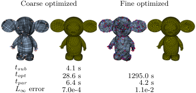
We next employ our structure-preserving subdivision for -directional fields to compute coarse-to-fine curl-reduced fields. This allows us to compute fine-level rotationally-seamless parameterizations (where the direction identifies across cuts, but without perfect integer translations) with a very low integration error. We compute an -RoSy (with [Knöppel et al. 2013]) on the coarse mesh, optimize it to be (approximately) curl-free with [Diamanti et al. 2015], and compute a coarse paramaterization that consequently has a very small integration error. The subdivision preserves the small amount of curl, and the fine-level parameterization also has a small error as a result. We compare this process to performing the curl-free optimization on the fine mesh directly. Our coarse-to-fine optimization is faster in almost two orders of magnitude. We demonstrate this in Figure 24 and in the teaser (Figure 1).
9. Discussion
Convergence and smoothness
As we discuss in the auxiliary material, our subdivision stencils for and have a few degrees of freedom (after counting the commutation constraints) that we use to optimize the spectrum of the subdivision stencil, such that it converges in the limit since the subdominant eigenvalues are less than . We conjecture that since the fields are derivatives of smoothly-subdivided functions, they are then one level of smoothness lower in the limit. However, we leave a formal theoretical analysis of convergence and smoothness to future work. We believe that a better design practice might be to allow and to vary entirely, where the smoothness of all subdivision operators is optimized concurrently (similarly to [Huang and Schröder 2010]), rather than modify the existing schemes.
Dual formulation
Our space uses for the projection operator . Nevertheless, the entire formulation can be made with the perpendicular , using the non-conforming divergence and conforming curl. This can be beneficial to fluid simulation.
Preconditioning and its disadvantages
The mass matrices of SHM are generally more strongly positive-definite than those of the FEM in the coarse mesh. The reason is that the uniform and stationary subdivision operators average the mesh, and create better triangulations. Nevertheless, the fact that the subdivision does not commute with the fine mass matrix also creates the high-frequency divergence pollution in the subdivided fields. It is then worthwhile to try and explore alternatives that consider the mass matrices within the templates, to obtain precise fine Hodge decompositions.
Full multi-resolution processing
Our paper explores low-dimensional coarse-to-fine approximations. Moreover, the basis functions are not orthonormal as an eigenbasis, albeit considerably cheaper to obtain. Nevertheless, SHM can be augmented by incorporating biorthogonal subdivision wavelets [Lounsbery et al. 1997; Bertram 2004], to obtain exact multi-resolution representation of functions over the fine mesh, with the advantages of increasing locality—this could benefit applications such as solving diffusion problems.
Non-triangular meshes
The space is not well defined for non-planar polygonal meshes. Nevertheless, in the spirit of mimetic elements [Bossavit 1998], the space , with its null-sum constraint, is well-defined for any polygonal mesh, implicitly defining . As such, our framework can consider other subdivision operators (such as Catmull-Clark). We will explore this in future work.
General restriction operators
Finally, our setting is currently limited to subdivision surfaces. It could be beneficial to also allow for a multi-resolution setting on general fine meshes using simplification operators (such as quadratic-error-based simplification [Garland and Heckbert 1997]) as the restriction operators. This should prove challenging as the vertex- and face-based restrictions have to be defined first, but will allow a very general framework for directional-field processing on arbitrary triangle meshes.
10. Acknowledgements
The authors would like to thank Bettina Speckmann for her support, and furthermore Fernando de Goes, Nilima Nigam, Mirela Ben-Chen, Justin Solomon and Etienne Vouga for helpful discussions.
References
- [1]
- Azencot et al. [2013] Omri Azencot, Mirela Ben-Chen, Frédéric Chazal, and Maks Ovsjanikov. 2013. An Operator Approach to Tangent Vector Field Processing. Computer Graphics Forum 32, 5 (2013).
- Azencot et al. [2015] Omri Azencot, Maks Ovsjanikov, Frédéric Chazal, and Mirela Ben-Chen. 2015. Discrete Derivatives of Vector Fields on Surfaces – An Operator Approach. ACM Transactions on Graphics 34, 3 (May 2015).
- Babuška and Suri [1994] Ivo Babuška and Manil Suri. 1994. The P and H-P Versions of the Finite Element Method, Basic Principles and Properties. SIAM Rev. 36, 4 (Dec. 1994), 578–632. https://doi.org/10.1137/1036141
- Ben-Chen et al. [2010] Mirela Ben-Chen, Adrian Butscher, Justin Solomon, and Leonidas Guibas. 2010. On discrete killing vector fields and patterns on surfaces. Computer Graphics Forum 29, 5 (2010).
- Bertram [2004] M. Bertram. 2004. Biorthogonal Loop-subdivision Wavelets. Computing 72, 1-2 (April 2004), 29–39. https://doi.org/10.1007/s00607-003-0044-0
- Biermann et al. [2000] Henning Biermann, Adi Levin, and Denis Zorin. 2000. Piecewise Smooth Subdivision Surfaces with Normal Control. In Proceedings of the 27th Annual Conference on Computer Graphics and Interactive Techniques (SIGGRAPH ’00). ACM Press/Addison-Wesley Publishing Co., New York, NY, USA, 113–120. https://doi.org/10.1145/344779.344841
- Bommes et al. [2009] David Bommes, Henrik Zimmer, and Leif Kobbelt. 2009. Mixed-integer Quadrangulation. ACM Transactions on Graphics 28, 3 (2009).
- Bossavit [1998] Alain Bossavit. 1998. In Computational Electromagnetism, Alain Bossavit (Ed.). Academic Press, San Diego, 1 – 30. https://doi.org/10.1016/B978-012118710-1/50002-7
- Brandt [1977] Achi Brandt. 1977. Multi-Level Adaptive Solutions to Boundary-Value Problems. Math. Comp. 31, 138 (1977), 333–390.
- Brandt et al. [2016] Christopher Brandt, Leonardo Scandolo, Elmar Eisemann, and Klaus Hildebrandt. 2016. Spectral Processing of Tangential Vector Fields. Computer Graphics Forum 35 (2016).
- Campen et al. [2015] Marcel Campen, David Bommes, and Leif Kobbelt. 2015. Quantized Global Parametrization. ACM Transactions on Graphics 34, 6 (2015).
- Cirak et al. [2002] Fehmi Cirak, Michael J. Scott, Erik K. Antonsson, Michael Ortiz, and Peter Schröder. 2002. Integrated modeling, finite-element analysis, and engineering design for thin-shell structures using subdivision. Computer-Aided Design 34, 2 (2002), 137–148.
- Crane et al. [2013] Keenan Crane, Fernando de Goes, Mathieu Desbrun, and Peter Schröder. 2013. Digital Geometry Processing with Discrete Exterior Calculus. In ACM SIGGRAPH 2013 Courses (SIGGRAPH ’13).
- Crane et al. [2010] Keenan Crane, Mathieu Desbrun, and Peter Schröder. 2010. Trivial Connections on Discrete Surfaces. Computer Graphics Forum 29, 5 (2010).
- Crouzeix and Raviart [1973] Michel Crouzeix and Pierre-Arnaud Raviart. 1973. Conforming and nonconforming finite element methods for solving the stationary Stokes equations I. ESAIM: Mathematical Modelling and Numerical Analysis - Modélisation Mathématique et Analyse Numérique 7, R3 (1973), 33–75. http://eudml.org/doc/193250
- Dahmen [1986] Wolfgang Dahmen. 1986. Subdivision algorithms converge quadratically. J. Comput. Appl. Math. 16, 2 (1986), 145 – 158. https://doi.org/10.1016/0377-0427(86)90088-9
- de Berg et al. [2008] Mark de Berg, Otfried Cheong, Marc van Kreveld, and Mark Overmars. 2008. Computational Geometry: Algorithms and Applications (3rd ed.). Springer-Verlag TELOS, Santa Clara, CA, USA.
- de Goes et al. [2016b] Fernando de Goes, Mathieu Desbrun, Mark Meyer, and Tony DeRose. 2016b. Subdivision Exterior Calculus for Geometry Processing. ACM Trans. Graph. 35, 4, Article 133 (July 2016), 11 pages. https://doi.org/10.1145/2897824.2925880
- de Goes et al. [2016a] Fernando de Goes, Mathieu Desbrun, and Yiying Tong. 2016a. Vector Field Processing on Triangle Meshes. In ACM SIGGRAPH 2016 Courses (SIGGRAPH ’16). ACM, New York, NY, USA, Article 27, 49 pages. https://doi.org/10.1145/2897826.2927303
- de Goes et al. [2014] Fernando de Goes, Beibei Liu, Max Budninskiy, Yiying Tong, and Mathieu Desbrun. 2014. Discrete 2-Tensor Fields on Triangulations. Computer Graphics Forum 33, 5 (2014).
- Desbrun et al. [2005] M. Desbrun, A. N. Hirani, M. Leok, and J. E. Marsden. 2005. Discrete Exterior Calculus. (2005). preprint, arXiv:math.DG/0508341.
- Diamanti et al. [2014] Olga Diamanti, Amir Vaxman, Daniele Panozzo, and Olga Sorkine-Hornung. 2014. Designing -PolyVector Fields with Complex Polynomials. Computer Graphics Forum 33, 5 (2014).
- Diamanti et al. [2015] Olga Diamanti, Amir Vaxman, Daniele Panozzo, and Olga Sorkine-Hornung. 2015. Integrable PolyVector Fields. ACM Transactions on Graphics 34, 4 (2015).
- Garland and Heckbert [1997] Michael Garland and Paul S. Heckbert. 1997. Surface Simplification Using Quadric Error Metrics. In Proceedings of SIGGRAPH. 209–216.
- Grinspun et al. [2002] Eitan Grinspun, Petr Krysl, and Peter Schröder. 2002. CHARMS: A Simple Framework for Adaptive Simulation. ACM Trans. Graph. 21, 3 (July 2002), 281–290. https://doi.org/10.1145/566654.566578
- Hertzmann and Zorin [2000] Aaron Hertzmann and Denis Zorin. 2000. Illustrating smooth surfaces. In Proc. SIGGRAPH 2000.
- Hirani [2003] Anil N Hirani. 2003. Discrete exterior calculus. Ph.D. Dissertation. California Institute of Technology.
- Huang and Schröder [2010] Jinghao Huang and Peter Schröder. 2010. sqrt(3) -Based 1-Form Subdivision. In Curves and Surfaces - 7th International Conference, Avignon, France, June 24-30, 2010, Revised Selected Papers. 351–368. https://doi.org/10.1007/978-3-642-27413-8_22
- Hughes et al. [2005] T.J.R. Hughes, J.A. Cottrell, and Y. Bazilevs. 2005. Isogeometric analysis: CAD, finite elements, NURBS, exact geometry and mesh refinement. Computer Methods in Applied Mechanics and Engineering 194, 39 (2005), 4135–4195. https://doi.org/10.1016/j.cma.2004.10.008
- Jüttler et al. [2016] Bert Jüttler, Angelos Mantzaflaris, Ricardo Perl, and Martin Rumpf. 2016. On numerical integration in isogeometric subdivision methods for PDEs on surfaces. Computer Methods in Applied Mechanics and Engineering 302 (2016), 131–146. https://doi.org/10.1016/j.cma.2016.01.005
- Kälberer et al. [2007] Felix Kälberer, Matthias Nieser, and Konrad Polthier. 2007. QuadCover - Surface Parameterization using Branched Coverings. Computer Graphics Forum 26, 3 (2007).
- Knöppel et al. [2013] Felix Knöppel, Keenan Crane, Ulrich Pinkall, and Peter Schröder. 2013. Globally optimal direction fields. ACM Transactions on Graphics 32, 4 (2013).
- Liu et al. [2016] Bei-Bei Liu, Yiying Tong, Fernando de Goes, and Mathieu Desbrun. 2016. Discrete Connection and Covariant Derivative for Vector Field Analysis and Design. ACM Transactions on Graphics 35, 3 (2016).
- Liu et al. [2014] Songrun Liu, Alec Jacobson, and Yotam Gingold. 2014. Skinning Cubic Bézier Splines and Catmull-Clark Subdivision Surfaces. ACM Trans. Graph. 33, 6, Article 190 (Nov. 2014), 9 pages. https://doi.org/10.1145/2661229.2661270
- Liu et al. [2006] Yang Liu, Helmut Pottmann, Johannes Wallner, Yong-Liang Yang, and Wenping Wang. 2006. Geometric Modeling with Conical Meshes and Developable Surfaces. ACM Transactions on Graphics 25, 3 (2006).
- Loop [1987] Charles Teorell Loop. 1987. Smooth subdivision surfaces based on triangles. Master’s thesis, University of Utah, Department of Mathematics.
- Lounsbery et al. [1997] Michael Lounsbery, Tony D. DeRose, and Joe Warren. 1997. Multiresolution Analysis for Surfaces of Arbitrary Topological Type. ACM Trans. Graph. 16, 1 (Jan. 1997), 34–73. https://doi.org/10.1145/237748.237750
- Mullen et al. [2011] P Mullen, A McKenzie, D Pavlov, L Durant, Y Tong, E Kanso, JE Marsden, and M Desbrun. 2011. Discrete Lie advection of differential forms. Foundations of Computational Mathematics 11, 2 (2011).
- Myles and Zorin [2012] Ashish Myles and Denis Zorin. 2012. Global Parametrization by Incremental Flattening. ACM Transactions on Graphics 31, 4 (2012).
- Nguyen et al. [2014] Thien Nguyen, Keçstutis Karc̆iauskas, and Jörg Peters. 2014. A Comparative Study of Several Classical, Discrete Differential and Isogeometric Methods for Solving Poisson’s Equation on the Disk. Axioms 3, 2 (2014), 280–299. https://doi.org/10.3390/axioms3020280
- Poelke and Polthier [2016] Konstantin Poelke and Konrad Polthier. 2016. Boundary-aware Hodge Decompositions for Piecewise Constant Vector Fields. Comput. Aided Des. 78, C (Sept. 2016), 126–136. https://doi.org/10.1016/j.cad.2016.05.004
- Polthier and Preuß [2003] Konrad Polthier and Eike Preuß. 2003. Identifying Vector Field Singularities Using a Discrete Hodge Decomposition. In Visualization and Mathematics III.
- Prautzsch et al. [2002] Hartmut Prautzsch, Wolfgang Boehm, and Marco Paluszny. 2002. Bezier and B-Spline Techniques. Springer-Verlag, Berlin, Heidelberg.
- Ray et al. [2008] Nicolas Ray, Bruno Vallet, Wan Chiu Li, and Bruno Lévy. 2008. N-symmetry Direction Field Design. ACM Transactions on Graphics 27, 2 (2008).
- Roy et al. [2018] Lawrence Roy, Prashant Kumar, Sanaz Golbabaei, Yue Zhang, and Eugene Zhang. 2018. Interactive Design and Visualization of Branched Covering Spaces. IEEE Transactions on Visualization and Computer Graphics 24, 1 (Jan 2018), 843–852. https://doi.org/10.1109/TVCG.2017.2744038
- Sageman-Furnas et al. [2019] Andrew Sageman-Furnas, Albert Chern, Mirela Ben-Chen, and Amir Vaxman. 2019. Chebyshev Nets from Commuting PolyVector Fields. ACM Trans. Graph. 38, 6 (Nov. 2019).
- Schober and Kasper [2007] Marc Schober and Manfred Kasper. 2007. Comparison of hp-adaptive methods in finite element electromagnetic wave propagation. COMPEL - The international journal for computation and mathematics in electrical and electronic engineering 26, 2 (2007), 431–446. https://doi.org/10.1108/03321640710727782
- Sharp et al. [2019] Nicholas Sharp, Yousuf Soliman, and Keenan Crane. 2019. The Vector Heat Method. ACM Trans. Graph. 38, 3 (2019).
- Shoham et al. [2019] Meged Shoham, Amir Vaxman, and Mirela Ben-Chen. 2019. Hierarchical Functional Maps between Subdivision Surfaces. Comput. Graph. Forum 38, 5 (2019), 55–73.
- Solomon et al. [2014] Justin Solomon, Raif Rustamov, Leonidas Guibas, and Adrian Butscher. 2014. Earth Mover’s Distances on Discrete Surfaces. ACM Trans. Graph. 33, 4, Article 67 (July 2014), 12 pages. https://doi.org/10.1145/2601097.2601175
- Stam [2003] Jos Stam. 2003. Flows on Surfaces of Arbitrary Topology. ACM Trans. Graph. 22, 3 (July 2003), 724–731. https://doi.org/10.1145/882262.882338
- Strang and Fix [2008] Gilbert Strang and George Fix. 2008. An Analysis of the Finite Element Method. Wellesley-Cambridge Press.
- Thomaszewski et al. [2006] Bernhard Thomaszewski, Markus Wacker, and Wolfgang Strasser. 2006. A Consistent Bending Model for Cloth Simulation with Corotational Subdivision Finite Elements. In Proceedings of the 2006 ACM SIGGRAPH/Eurographics Symposium on Computer Animation (SCA ’06). Eurographics Association, Aire-la-Ville, Switzerland, Switzerland, 107–116. http://dl.acm.org/citation.cfm?id=1218064.1218079
- Tong et al. [2003] Yiying Tong, Santiago Lombeyda, Anil N. Hirani, and Mathieu Desbrun. 2003. Discrete Multiscale Vector Field Decomposition. ACM Transactions on Graphics 22, 3 (2003), 445–452.
- Vaxman et al. [2019] Amir Vaxman et al. 2019. Directional: A library for Directional Field Synthesis, Design, and Processing. https://doi.org/10.5281/zenodo.3338175 https://github.com/avaxman/Directional.
- Vaxman et al. [2016] Amir Vaxman, Marcel Campen, Olga Diamanti, Daniele Panozzo, David Bommes, Klaus Hildebrandt, and Mirela Ben-Chen. 2016. Directional Field Synthesis, Design, and Processing. Computer Graphics Forum 35, 2 (2016), 545–572. https://doi.org/10.1111/cgf.12864
- Wang et al. [2006] Ke Wang, Yiying Tong, Mathieu Desbrun, Peter Schröder, et al. 2006. Edge subdivision schemes and the construction of smooth vector fields. ACM Transactions on Graphics 25, 3 (2006).
- Wardetzky [2006] Max Wardetzky. 2006. Discrete Differential Operators on Polyhedral Surfaces–Convergence and Approximation. Ph.D. Dissertation. Freie Universität Berlin.
- Zadravec et al. [2010] Mirko Zadravec, Alexander Schiftner, and Johannes Wallner. 2010. Designing Quad-dominant Meshes with Planar Faces. Computer Graphics Forum 29, 5 (2010).
- Zhang et al. [2006] Eugene Zhang, Konstantin Mischaikow, and Greg Turk. 2006. Vector Field Design on Surfaces. ACM Transactions on Graphics 25, 4 (2006).
Appendix A as inverse of
We next show that tangential vector fields are preserved under the operation .
Let be the CCW oriented edges of a face in CCW order (i.e., ), and let be the angle opposite the corresponding edge. Here, we will interpret as column vectors. Consider a tangential vector field, that is locally defined on a triangle as , without loss of generality. Then,
| (31) |
Applying , we get
| (32) | ||||
| (33) | ||||
| (34) | ||||
| (35) |
where we renamed the summed terms in the brackets for convenience. Note that . We can express in terms of via orthogonal decomposition
| (36) |
which allows us to write
| (37) | ||||
| (38) | ||||
| (39) |
where we use . Similarly,
| (40) | ||||
| (41) | ||||
| (42) |
Working out , we get
| (43) | ||||
| (44) | ||||
| (45) | ||||
| (46) |
where we use and for the interior angles of a triangle. For , we get
| (47) | ||||
| (48) | ||||
| (49) |
combining gives:
| (50) |
as desired.
To generalize this result for arbitrarily oriented edges, we need to multiply and by their appropriate sign, and sign the values to be correctly oriented. This amounts to
| (51) |
as stated before.
Appendix B Inner Product on
In the following, we develop the inner product mass matrix , to prove the formulation of Equation 14.
Consider a face with three edges that are, without loss of generality, positively oriented towards the face. Further consider two halfedge forms restricted to the face on these edges: and , representing respective face-based vectors and . We “pack” their representation to edges and alone, and by so trivially encoding the null-sum constraint (and resp. for ). Following Equation 13, we have that the inner product , restricted to the face, is given by:
This reproduces the inner product between and in the face . We then get that:
Consider the angles opposite to edges . Then, we use the identities:
for any cyclic shift of . Then we get:
where we use the unpacking operator .
Appendix C Stencils
In the following we details our subdivision stencils and the way we derived them. We modified the integrated face-based subdivision operator, derived from the DEC in SEC [de Goes et al. 2016b], to accommodate for our boundary conditions, and consequently had to modify around boundary vertices. In addition, we introduced a subdivision for unsigned integrated edge functions . We denote the number of incident faces as , so that the regular interior stencils have and the regular boundary stencils have . In addition, we denote boundary vertices by a black dot and an interior vertex by an open dot.
C.1. Loop subdivision
For , we chose Loop subdivision (Fig. 25) with
| (52) |
following Biermann et al. [Biermann et al. 2000]. The templates can be found in Figure 25. Similar to de Goes et al. [de Goes et al. 2016b], we chose to keep the odd stencil next to the boundary the same as the interior stencil.
C.2. Halfbox spline subdivision
For the halfbox spline subdivision operator , we use the same stencils as Wang et al. [Wang et al. 2006] for the interior faces, as given by Figure 26. Due to the extra constraints on at the boundary, we modified the boundary stencils for . The parameters of the interior stencils are given by
| (53) | ||||
| (54) | ||||
| (55) |
where is the halfbox spline parameter, given by
| (56) |
C.3. 1-form subdivision operator
For completeness, we list the coefficients for the interior stencils of the subdivision operator, as used in deGoes et al. [de Goes et al. 2016b].
| (57) | ||||
| (58) | ||||
| (59) | ||||
| (60) | ||||
| (61) | ||||
| (62) |
with the coeffficents for Loop resp. halfbox spline subdivision, as defined before.
C.4. Stencil Constraints
The subdivision operators were created with mirror symmetric templates about the target mesh element. The following commutation relations were imposed
C.4.1. Interior stencils of
For constructing the interior stencils of , we assume that the stencil coefficients are mirror-symmetric with respect to the subdivided edge element. In addition, as in [Wang et al. 2006], we fix the odd stencil for with the same global shape as the odd stencil. Finally, we demand that the coefficients for even stencils of valence are the same over the finite support of .
After construction of the new operator via the commutations, there are three degrees of freedom remaining. We resolve two of them by requiring all coefficients of the even valence 6 stencil to be positive. The remaining degree of freedom is present in the valence 4 even stencil, for which the local subdivision operator spectrum is , where is the remaining degree of freedom. We choose to make the spectrum consist of .

The stencils of the operator are summarized in Figure 28. The coefficients and for the valence 5 interior rings are given by
| (63) |
C.5. Boundary stencils
We assume all boundary stencils to be applied with mirror symmetry around the boundary. Since we want to preserve the condition on the boundary, we demand that the coefficients for the boundary stencil for even elements of solely depend on the boundary. In addition, we require that the odd stencil for the elements that touch the boundary with one of their vertices remains the same for . Using these assumptions on the stencils, we solve for , and in conjunction. The resulting subdivision operators have a single degree of freedom left, which we resolve by requiring all elements to be positive. The modified stencils for are shown in Figure 26, for in Figure 27, and for in Figure 28.