Unrooted non-binary tree-based phylogenetic networks
Abstract
Phylogenetic networks are a generalization of phylogenetic trees allowing for the representation of non-treelike evolutionary events such as hybridization. Typically, such networks have been analyzed based on their ‘level’, i.e. based on the complexity of their 2-edge-connected components. However, recently the question of how ‘treelike’ a phylogenetic network is has become the center of attention in various studies. This led to the introduction of tree-based networks, i.e. networks that can be constructed from a phylogenetic tree, called the base tree, by adding additional edges. While the concept of tree-basedness was originally introduced for rooted phylogenetic networks, it has recently also been considered for unrooted networks. In the present study, we compare and contrast findings obtained for unrooted binary tree-based networks to unrooted non-binary networks. In particular, while it is known that up to level 4 all unrooted binary networks are tree-based, we show that in the case of non-binary networks, this result only holds up to level 3.
Keywords: phylogenetic tree, phylogenetic network, tree-based network, level- network, Hamiltonian path
Email address: email@mareikefischer.de (Mareike Fischer)
1 Introduction
Traditionally, phylogenetic trees have been used in order to represent the evolutionary history of sets of species. However, the evolution of species is not always tree-like, in particular if they have been subject to reticulation events like hybridization or horizontal gene transfer. Thus, phylogenetic networks have come to the fore as a mathematical generalization of phylogenetic trees, allowing for the representation of non-tree-like evolutionary events.
Mathematically, unrooted phylogenetic networks are connected, simple graphs containing degree-1 vertices (representing present-day species) that are not necessarily acyclic, as reticulation events may lead to 2-edge-connected components in the graph. In this regard, Choya et al (2005) introduced the concept of level- networks. These are networks in which in each 2-edge-connected component the number of edges which need to be removed to turn them into trees is at most . In this sense, the level measures the complexity of a network. So the smaller the level, the more ‘treelike’ the network.
However, while a network can contain various trees, not all networks are suitable to explain the evolution of present-day species to the same extent. This is due to the fact that some networks contain no support tree (Francis and Steel (2015)). A support tree is a spanning tree that has the same leaf set as the network, i.e. it represents the evolution of the same present-day species as the given network. Biologically, these networks are most relevant, because the leaves typically represent the species for which one has data (e.g. DNA sequences) and on which the reconstruction of evolution is based.
So given a phylogenetic network, it is of high interest to study its ‘treelikeness’, and in terms of support trees, this reduces to the question whether the network is merely a tree with additional edges. While Francis and Steel (2015) introduced the concept of tree-basedness for rooted binary phylogenetic networks, recently Francis et al (2018b) extended it to unrooted binary networks, Jetten and van Iersel (2018) to rooted non-binary networks and Hendriksen (2018) to unrooted non-binary networks.
In the present manuscript, we focus on unrooted non-binary networks and link and contrast our findings to results recently obtained for unrooted binary networks by Francis et al (2018b). In particular, we show that while up to level 4 all unrooted binary networks are tree-based (Theorem 1 in Francis et al (2018b), in case of non-binary networks, this result only holds up to level 3 (Theorem 1 of the present manuscript). More precisely, there are non-binary level-4 networks that are not tree-based. This provides an answer to Question 5.3 posed in Hendriksen (2018), asking whether there are networks of level less than 5 that are not tree-based.11 1 Note that our definition of tree-based networks corresponds to the definition of loosely tree-based networks in Hendriksen (2018) (see Section 2.1 in the present manuscript), so the question is posed there in a slightly different way.
Our analysis of the relationship between the level of a non-binary network and its tree-basedness relies on certain properties of the graph underlying the network (e.g. the number of vertices in the ‘blobs’ of the network). A similar analysis can also be used to show that all unrooted binary networks up to level 4 are tree-based, i.e. to re-prove Theorem 1 of Francis et al (2018b). We provide the details of this alternative proof in the Appendix. Importantly, this allows us to show that there are precisely 2 ‘minimal’ (in the number of vertices) proper unrooted binary phylogenetic level-5 networks that are not tree-based; i.e. such networks are very rare.
The remainder of this manuscript is organized as follows. In Section 2, we introduce some basic phylogenetic and graph-theoretical concepts and terminology. In Section 3.1 we then consider several basic results obtained for unrooted binary networks in Francis et al (2018b) and generalize them to non-binary networks. We then use these results to state the main theorem of this paper saying that all unrooted non-binary networks up to level 3 are tree-based in Section 3.2. In Section 3.3 we re-visit the corresponding result for unrooted binary networks obtained by Francis et al (2018b) (Theorem 1 therein) and show that there are exactly two unrooted binary level-5 networks with 12 vertices that are not tree-based. Moreover, we provide an alternative proof of Theorem 1 in Francis et al (2018b) in the Appendix.
2 Preliminaries
2.1 Phylogenetic Concepts
Phylogenetic Networks
Throughout this manuscript we assume that is a finite set (e.g. of taxa or species) with . A non-binary unrooted phylogenetic network (on ) is a connected, simple graph with and no vertices of degree 2, where the set of degree 1 vertices (referred to as the leaves or taxa of the network) is bijectively labeled by and thus identified with . An unrooted phylogenetic network is called unrooted binary if every non-leaf vertex has degree 3.22 2 Note that, somewhat counterintuitively, the class of binary phylogenetic networks is contained in the class of non-binary ones, as non-binary ones are simply more general. This definition is common in the phylogenetic literature. In the following, we denote by the set of interior edges of , i.e. those edges that are not incident to a leaf.
Moreover, note that an unrooted phylogenetic tree is an unrooted phylogenetic network whose underlying graph structure is a tree.
Edge subdivision and vertex suppression
In order to discuss the notion of tree-basedness, we now need to introduce the concepts of subdividing an edge and suppressing a vertex. Therefore, let be a phylogenetic network with some edge . Then, we say that we subdivide by deleting , adding a new vertex and adding the edges and . The new degree 2 vertex is sometimes also referred to as an attachment point. Note that we often also refer to the vertex adjacent to a leaf as the attachment point of , even if this vertex has degree higher than two.
In contrast to adding vertices to a network, given a degree 2 vertex with adjacent vertices and , by suppressing we mean deleting and its two incident edges and and adding a new edge . Note that the resulting graph can be a multigraph, i.e. a graph that may contain parallel edges and/or loops (cf. Figure 1).

Tree-based networks
Edge subdivisions and attachment points play a fundamental role in the concept of tree-based networks. When tree-basedness was first introduced for rooted binary phylogenetic networks by Francis and Steel (2015), tree-based networks were constructed from rooted binary phylogenetic trees by subdividing edges and adding new edges between such pairs of attachment points. However, tree-based networks (whether they are rooted or unrooted, binary or non-binary) can alternatively be defined as follows. For technical purposes (e.g. for Lemma 3 in the Appendix), we first define tree-basedness for general (multi)graphs before defining it for phylogenetic networks (which are by definition simple graphs).
Definition 1.
Let be a connected (multi)graph and with leaf set , i.e. . is called tree-based if there is a spanning tree in (with ) whose leaf set is equal to . is then called a support tree (for ). Moreover, tree which can be obtained from by suppressing potential degree 2 vertices is called a base tree (for ). If is a phylogenetic network with leaf set and underlying graph and is tree-based, then we call a tree-based network with support tree (and base tree ).
Note that the existence of a support tree for implies the existence of a base tree for .
Moreover, note that while we consider only one kind of tree-basedness for unrooted non-binary networks, one might want to distinguish between several forms of tree-based networks, depending on different ways of introducing additional edges (cf. Hendriksen (2018)). For instance, Hendriksen (2018) distinguished between strictly tree-based, tree-based and loosely tree-based networks, where the class of loosely tree-based networks is the most general one, which contains the other two. The latter class, i.e. the one that Hendriksen (2018) calls the class of loosely tree-based, is precisely the class of networks we call tree-based in the present manuscript.
Cut edges/vertices, blobs, level- and proper networks
We will see in subsequent sections that it is often useful to decompose a phylogenetic network into simpler pieces, which can then be analyzed individually. Therefore, recall the following definitions from Gambette et al (2012). Let be an unrooted network. A cut edge, or bridge, of is an edge whose removal disconnects the graph, i.e. an edge such that is disconnected. Similarly, we call a vertex a cut vertex, if deleting and all its incident edges disconnects the graph.
A cut edge is called trivial if one of the connected components induced by the removal of the cut edge is a single vertex (which must necessarily be a leaf). Following Gambette et al (2012), we call a simple network if all of its cut edges are trivial. A blob in a network is a maximal connected subgraph that has no cut edge. If a blob consists only of one vertex, we call the blob trivial. Note that this implies that we can consider a network as a “tree-like structure” with blobs as vertices (cf. Figure 2). The idea of “blobbed trees” has already been introduced for rooted phylogenetic networks in Gusfield and Bansal (2005) and we use it for unrooted ones in the following. Moreover, note that in a binary network it can be easily seen that a blob not only contains no cut edges, but it contains no cut vertices either (because in binary networks, every cut vertex is incident to a cut edge, and these are excluded from blobs, cf. Lemma 6 in the Appendix). In contrast, in the non-binary setting, a blob may contain cut vertices. An example for such a blob can be seen in Figure 2.

Recall that a binary network on is called proper (Francis et al (2018b)) if every cut edge induces a split of , i.e. a bipartition of into two non-empty subsets. Here, however, we call a network proper if the removal of any cut edge or cut vertex present in the network leads to connected components containing at least one leaf each. Note that this definition of proper networks generalizes the one given in (Francis et al, 2018b) to the non-binary case. There, only cut edges were considered for proper networks. However, the alteration of the definition in the non-binary case is needed in order to exclude some networks which cannot be tree-based. In particular, we exclude non-tree networks in which all leaves are attached to the same interior vertex.
Remark 1.
A network which is not a tree and for which such that all leaves are attached to the same interior vertex cannot be tree-based. This is due to the fact that any spanning tree will induce additional leaves that are not part of , i.e. no spanning tree of the network is a support tree (cf. Figure 3). Moreover, note that a network with and cannot be proper, because if no cut edge or cut vertex can induce a partition of the taxon set.

Given a network on and an integer , we call a level- network if at most edges have to be removed from each blob of to obtain a tree.
Moreover, following Francis et al (2018b), given a network and a blob in , we define a simple network by taking the union of and all cut edges in incident with vertices in , where the leaf set of is simply the set of end vertices of these cut edges that are not already a vertex in .
2.2 Graph-theoretical concepts
Besides the phylogenetic terminology, we need to introduce some basic concepts from classical graph theory before we can proceed with analyzing the tree-basedness of unrooted phylogenetic networks. In particular, we need the notion of cubic graphs and Hamiltonian paths/cycles.
A cubic graph is a graph such that all vertices have degree 3. We will now show that both cubic graphs and unrooted binary phylogenetic networks necessarily contain an even number of vertices, a property that will be useful later on (e.g. in the proof of Lemma 7).
Proposition 1.
Let be a cubic graph. Then, contains an even number of vertices. Furthermore, if is an unrooted binary phylogenetic network with leaves, also contains an even number of vertices.
Proof.
The first part of the statement follows from the so-called handshaking lemma (Harris et al, 2000, Theorem 1.1), which states that . Thus, as is a cubic graph, we have that three times the number of vertices of equals two times the number of edges in , i.e. . Therefore, we have , which (as is an integer) implies that for some . Thus, we have , which shows that has an even number of vertices.
Similarly, by applying the handshaking lemma for an unrooted binary phylogenetic network on with , we have that
In particular, , and thus the number of vertices in is even. ∎
Another well-known graph theoretical concept we wish to introduce here is a Hamiltonian path. A Hamiltonian path is simply a path in a graph that visits each vertex exactly once. If this path is a cycle, the Hamiltonian path is called a Hamiltonian cycle. A graph that contains a Hamiltonian cycle is called a Hamiltonian graph. As has been noted in Francis et al (2018b) and as we will elaborate in the present manuscript, Hamiltonian paths play an important role concerning the tree-basedness of phylogenetic networks.
3 Results
The main aim of this section is to show that all unrooted non-binary phylogenetic networks up to level 3 are tree-based, whereas unrooted non-binary level-4 networks are not necessarily tree-based. However, we first state some preliminary results from the literature for binary networks and show that they also hold for non-binary networks.
3.1 Basic results
In this section, we first state some basic results that will be needed throughout this manuscript. Some of them are extensions of the results presented in Francis et al (2018b) from the binary to the non-binary case.
We start by considering the following lemma by Francis et al (2018b), which states a close relationship for binary networks between the properties of being tree-based and being proper. In particular, a non-proper phylogenetic network cannot be tree-based.
Lemma 1 (Francis et al (2018b)).
If is an unrooted binary tree-based network, then every cut edge of induces a split of , i.e. is proper.
Note that in the non-binary case, the absence of cut edges need not imply that the network is proper, because it might still contain cut vertices. So we now generalize this lemma to non-binary networks.
Lemma 2.
If is an unrooted tree-based network (binary or not), then is proper.
Proof.
Let be an unrooted tree-based network. Then, it contains a support tree whose leaf set coincides with . As is a spanning tree of , its vertex set contains any possible cut vertex , and if is a cut edge of , it must also occur in the spanning tree (otherwise could not be connected). Let be the base tree corresponding to . Now, as any phylogenetic tree is clearly a proper phylogenetic network, in particular is proper. Note that this implies that , too, must have the property that the removal of any cut edge or cut vertex will subdivide , because is like , just possibly with additional degree-2 vertices. Thus, removing any cut vertex or cut edge from results in connected components containing at least one leaf of (and thus of ) each. But as contains all cut vertices and cut edges of , the same must hold for . In particular, is proper. ∎
We next state some general results concerning the decomposition of unrooted networks into simpler parts and the number of vertices in a blob.
Francis et al (2018b) prove a decomposition theorem for tree-based unrooted binary networks based on the simple networks associated with blobs introduced above. This can directly be generalized to non-binary networks and we have the following statement.
Proposition 2.
Suppose is an unrooted network. Then is tree-based if and only if is tree-based for every blob in .
Our proof of this proposition is very similar to the proof of Proposition 1 in Francis et al (2018b) and Proposition 2.9 in Hendriksen (2018). However, as we explicitly allow blobs to contain cut vertices, we shortly outline the proof in the Appendix.
Roughly speaking, Proposition 2 states that it is sufficient to analyze all blobs of an unrooted network individually in order to decide whether a network is tree-based or not.
As we will show subsequently, it also often makes sense to consider (simple) networks with only two leaves. Therefore, we first recall a useful observation of Francis et al (2018b), which is, again, also valid for non-binary networks.
Lemma 3.
Let be a network on with . For any let denote the network obtained from by deleting and its incident edge, and suppressing the potentially resulting degree-2 vertex. Then, if is tree-based, so is .
The proof of this lemma is very similar to the proof of Lemma 3 in Francis et al (2018b). However, as we are not only considering binary networks, but also non-binary ones, and as we – unlike Francis et al (2018b) – explicitly consider the case of parallel edges, we give the proof again in the Appendix. In any case it should be noted that might not be a phylogenetic network as it might contain parallel edges. This is why in Definition 1 tree-basedness is also defined for (multi)graphs.
Remark 2.
Note that the converse does not necessarily hold, i.e. if is tree-based, does not necessarily have to be tree-based, whether is binary or not. To see this, consider the network depicted in Figure 4. Note that this example is extreme in the following sense: It shows that even if a tree-based network is binary and contains only one blob and even if does not contain any cut vertices and no cut edges other than the ones incident to leaves, it might not be possible to remove any leaf and suppress the resulting degree-2 vertex without losing tree-basedness. In particular, there exists no pair of two leaves in this network such that it is still tree-based.
Note that this extreme example is based on the graph shown in Figure 5(a), which we found in Zamfirescu (1976). There, it is proven that any longest path in this graph of 12 vertices has length 10.
Consider Figure 5(b). Note that this graph of 9 vertices, which contains three degree-2 vertices, is Hamiltonian, i.e. it contains a Hamiltonian cycle.33 3 In fact, as proven in Zamfirescu (1976), deleting all leaves of this graph corresponds to deleting one vertex from the famous Petersen graph, which is hypohamiltonian. However, it does not contain a Hamiltonian path from either one of these three degree-2 vertices to another one of those: If it did, this path would have length 9 as it would have to cover all 9 vertices, and it could easily be extended by 2 in the graph of Figure 5(a) by re-attaching the leaves. This would give a total path of length 11 in the Zamfirescu graph of Figure 5(a), which does not exist as the maximal path length there is 10.
Now our network in Figure 4 basically consists of two copies and of the graph of Figure 5(b), which are connected by three paths. One of the connecting paths does not have an adjacent leaf. Suppose there was a support tree using only edges of two of these connecting paths. Then this support tree would imply a path through, say, , which would imply a Hamiltonian path in the graph of Figure 5(b) from one degree-2 vertex to another one – a contradiction, as we have seen above that such a path cannot exist. Therefore, it is clear that in , edges of all three paths connecting and must be used by any support tree. In fact, as this argument holds for both and , in each of the three paths, any support tree must contain an edge incident to and an edge incident to . As the dashed edge in Figure 4 is therefore contained in any support tree of , the induced spanning trees of and are already connected. Thus, using an entire path of the remaining two connecting paths would necessarily induce a cycle, which is not allowed. So there must be at least one edge on both these remaining connecting paths from to which is not covered by any support tree (this is, in fact, the edge between the attachment points of the two leaves of each of these paths). Thus, removing any leaf and suppressing its respective attachment point would necessarily destroy tree-basedness.


We now present another observation that will be useful in the following, namely that the number of vertices in a non-trivial blob incident with at most two cut edges is bounded by in a level- network, where .
Lemma 4.
Let be an unrooted level- network (not necessarily binary) with , let be a non-trivial blob, and assume that there are at most two cut edges in incident to . Let denote the number of vertices in . Then,
Proof.
We first show that . Let denote the number of edges in . As we assumed that there are at most two cut edges in incident to , can have at most two degree-2 vertices. All other vertices are of degree at least (they can be higher, as we do not assume that the network is binary). Thus, using the handshaking lemma, we have
On the other hand, as we are considering simple graphs, can have at most edges. Thus,
which leads to
This inequality is fulfilled if or if . As is a positive integer, we conclude .
Next, we need to show that for . Recall that an unrooted tree on vertices has edges. As is a level- network, at most edges have to be removed from to obtain a tree. Thus, . In other words, . Using the lower bound for from above, we derive
and thus in particular . This completes the proof. ∎
3.2 Unrooted non-binary tree-based networks
We are now in the position to state the main result of this paper, namely the fact that all proper unrooted non-binary phylogenetic networks up to level 344 4 Note that by definition, all networks of level less than 3 are contained in the class of level-3 networks. are tree-based, whereas unrooted non-binary level-4 networks are not necessarily tree-based.
Theorem 1.
All proper unrooted non-binary unrooted level-3 are tree-based. Moreover, unrooted non-binary networks of level greater than 3 need not be tree-based.
In order to prove Theorem 1, we need the following lemma, which gives a lower bound on the number of vertices needed to destroy tree-basedness.
Lemma 5.
Any minimal (in the number of vertices) proper unrooted non-binary non-tree-based network has 6 interior vertices and 2 leaves, i.e. 8 vertices in total.
Proof.
It suffices to show that all proper unrooted non-binary networks on less than 8 vertices are tree-based. In this regard, we performed an exhaustive search using Mathematica (Inc., 2017). In the following we explain the details of this exhaustive search.
First of all, we obtained a list containing all simple graphs with up to 7 vertices from the “House of Graphs” database (cf. Brinkmann et al (2013)).
We then filtered these graphs for networks and thus excluded unconnected graphs, graphs without leaves (i.e. vertices of degree 1) as well as graphs with vertices of degree 2.
We then further excluded all non-proper networks by checking whether the removal of any cut edge or any cut vertex present in the network resulted in connected components containing at least one leaf each.
This left us with 28 proper unrooted non-binary networks, which can all easily be shown to be tree-based. We depicted all of them in the Appendix (see catalog of all proper tree-based networks with up to 7 vertices in Figures VII and VIII).
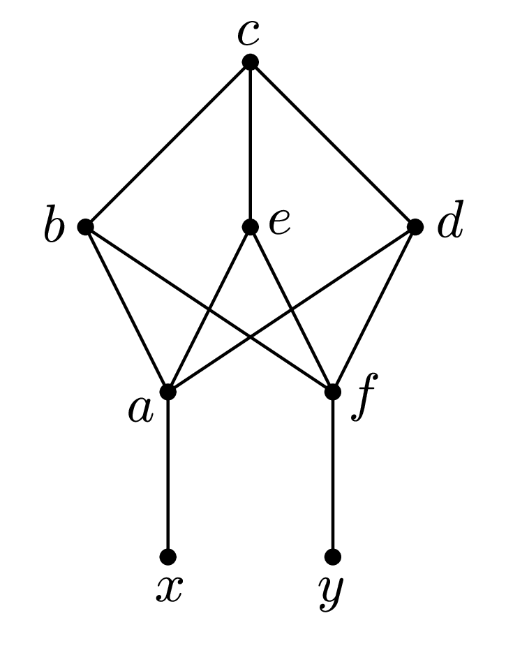
This shows that all unrooted non-binary networks with up to 7 vertices are tree-based. However, for 8 vertices there exist unrooted non-binary networks which are not tree-based. One such example is depicted in Figure 6. This network has 6 interior vertices and 2 leaves and it can be seen not to be tree-based as follows. If it was tree-based, then there would be a path from to visiting each vertex exactly once. Trivially, this path must start with edge and end with edge . Now, the first three vertices of the path must either be or . In all cases, the 4th vertex must be , because the only other vertex (except from ) that can be reached from or is ; however, has to be visited second last. Thus, so far we either have a path starting or . Consider the first case, i.e. . From we can either go to or to . If we go to , i.e. if we have , the only “free” vertex reachable from is . This leads to a contradiction as vertex has not been visited. If we instead go to , i.e. if we have , the only “free” vertex reachable from again , which causes a contradiction as has not been visited. Similar contradictions follow for all other cases. This completes the proof. ∎
We are now in the position to prove Theorem 1.
Proof (Theorem 1).
We have to show that all proper unrooted non-binary phylogenetic networks of levels are tree-based. Note that if contains only one leaf, either the underlying network consists of a single vertex (and is thus trivially tree-based) or it is not proper (Remark 1). This is why we now consider only networks with .
Recall that we can decompose into a collection of simple networks associated with the non-trivial blobs in , each having at least two leaves, and if each of these simple networks is tree-based, then so is by Proposition 2. (Note that trivial blobs are generally tree-based, which is why we only consider non-trivial blobs and their associated networks ). Moreover, if we remove all but 2 leaves from each of these simple networks and obtain a tree-based network, then must have been tree-based due to Lemma 3.
Now, for , the statement holds, as a level-0 network is a tree and thus tree-based. For , we know that at most one edge has to be removed from each non-trivial blob of to obtain a tree. Removing at most one edge from each such non-trivial blob of , however, cannot induce any new leaves (if an interior vertex of some blob became a leaf after removing one edge from this blob, this would imply that this vertex is a degree-2 vertex in , which is not allowed. Thus, the tree that we obtain from removing at most one edge from each non-trivial blob in a level-1 network can directly be considered a support tree for . This implies that level-1 networks are always tree-based.
Let us now consider . By Lemma 5, we know that any simple network that leads to a proper non-binary non-tree-based network has to have at least 6 interior vertices and 2 leaves, i.e. at least 8 vertices in total. Moreover, by Lemma 4 we know that for , the number of vertices in a non-trivial blob associated with a network is bounded from above by , i.e. in case of level 2, the maximum number of vertices in is 4. This implies that there cannot exist a level-2 network that is not tree-based.
In order to prove that there also does not exist a non-tree-based level-3 network, we exhaustively generated all unrooted proper phylogenetic networks on 8 vertices, analyzed them for tree-basedness and computed their level. This exhaustive search was conducted in the following way: We used the “House of Graphs” database (cf. Brinkmann et al (2013)) to obtain a list of all graphs with 8 vertices (12346 in total). These were then filtered for unrooted proper phylogenetic networks in the same way as described in the proof of Lemma 5, resulting in a total of 197 unrooted proper phylogenetic networks. These were then analyzed for tree-basedness and it turned out that there are only 8 proper phylogenetic networks on 8 vertices that are not tree-based (see Figure IX). However, none of them is a level-3 network, i.e. we can conclude that all proper non-binary level-3 networks are indeed tree-based.
Remark 3.
Note that the last part of the proof above answers a question posed in Hendriksen (2018), asking whether there exist networks of level less than 5 that are not loosely tree-based. As the definition of loosely tree-based in Hendriksen (2018) precisely corresponds to our definition of tree-based, the level-4 network depicted in Figure 6 provides such an example.
3.3 Unrooted binary tree-based networks
We now re-visit tree-basedness of unrooted binary phylogenetic networks, in order to re-establish a known result and in order to extend it by an additional proposition.
Recall that Francis et al (2018b) recently established the following result, which is the binary analog of our Theorem 1.
Theorem 2 (adapted from Francis et al (2018b)).
All proper unrooted binary level-4 network are tree-based. Moreover, networks of level greater than 4 need not be tree-based.
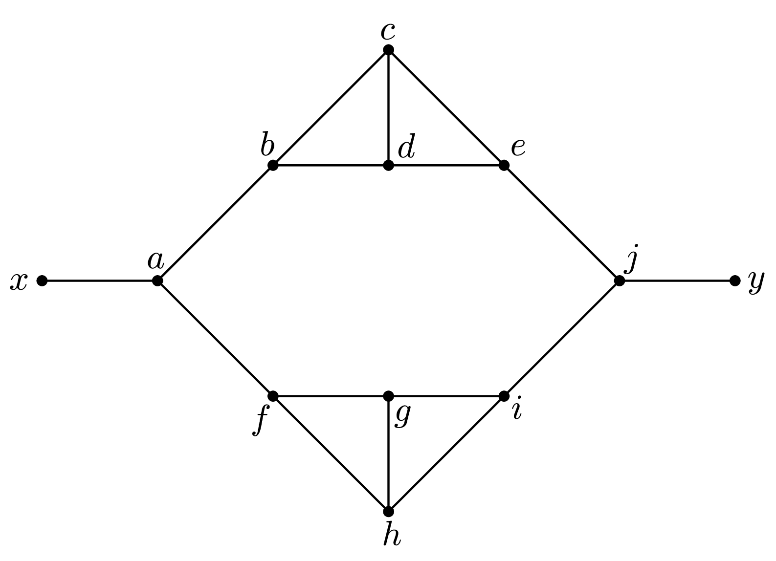
Note that the example given in Francis et al (2018b) for the second part of this theorem was unfortunately erroneous. Indeed, the level-5 network on depicted in Figure 7 was used in Francis et al (2018b) to show that level-5 networks need not be tree-based. However, this network in fact is tree-based as there exists a spanning tree in whose leaf set is equal to . While the authors have recently independently pointed out this error and published an erratum (Francis et al, 2018a), in the process of writing this manuscript we have further analyzed unrooted binary non-tree-based networks. Using a similar approach as in our proof of Theorem 1, we provide an alternative proof of Theorem 2, the details of which are given in the Appendix. More importantly, though, this analysis enabled us to show that binary non-tree-based level-5 networks are ‘rare’ in the sense stated by the following proposition.

Proposition 3.
There are precisely two minimal (in the number of vertices) proper unrooted binary phylogenetic level-5 networks that are not tree-based. Both of them contain exactly 12 vertices. In particular, all other proper unrooted binary phylogenetic level-5 networks that are not tree-based contain more than 12 vertices.
The proof of this proposition is given in the Appendix. The two minimal networks, however, are depicted in Figure 8.
Remark 4.
Note that both networks in 8 are symmetric in the sense that swapping their leaves and leads to an isomorphic network. So in fact, there are really only two minimal phylogenetic networks fulfilling the required properties from Proposition 3, even though our proof technique described in the Appendix is based on unlabeled graphs.
4 Discussion
The main aim of this manuscript was to generalize some of the results presented in Francis et al (2018b) for binary unrooted tree-based networks to non-binary ones. While some results are straightforward to generalize, others need to be adjusted. Differences between non-binary and binary networks include, for instance, that unlike in the binary case, level-4 networks need not necessarily be tree-based in the non-binary case. This provides the answer to Question 5.3 in Hendriksen (2018), asking whether there are non-binary networks of level less than 5 that are not tree-based.
While the main focus of this manuscript was on non-binary networks we also re-visited binary ones. In particular, we gave two examples showing that binary level-5 networks are not always tree-based, as the example given in Francis et al (2018b) was unfortunately erroneous. Even though one correct example has in the meantime independently been published by the authors in an erratum (cf. Francis et al (2018a)), our study additionally shows that binary level-5 networks that are not tree-based are ‘rare’ in the sense that there are only two minimal ones. Furthermore, our study provides an alternative proof for the fact that all proper unrooted binary networks up to level 4 are tree-based (Theorem 1 in Francis et al (2018b)).
Tree-based phylogenetic networks are an interesting topic for future research. Note that they are not only of high biological relevance – they also link mathematical phylogenetics to classic graph theory, like e.g. Hamiltonian paths and cycles, cubic graphs, and classic results like the ones in Zamfirescu (1976). But not only does the study of phylogenetic networks benefit from connections to classic graph theory – in fact, the opposite is also true: In graph theory and various applications, finding spanning trees with few leaves has been a topic of high interest (cf. Tsugaki and Yamashita (2007); Rivera-Campo (2012); Salamon and Wiener (2008)). Note that every connected graph has a spanning tree, and in all spanning trees, any vertices of the graph of degree 1 must be contained as leaves. So for phylogenetic networks, it is obvious that all leaves of the network are necessarily also leaves of any spanning tree. Tree-basedness, however, implies that there are no more leaves than this minimum requirement suggests. In this regard, support trees of tree-based phylogenetic networks are just spanning trees with the smallest possible number of leaves. Many techniques, like e.g. Hamiltonicity, which have already been used to classify spanning trees with few leaves (cf. Salamon and Wiener (2008)) are therefore also useful in the study of tree-basedness. We are sure that this connection to graph theory will prove fruitful for future studies, too.

Acknowledgement
We thank two anonymous reviewers of an earlier version of this manuscript for their valuable suggestions and feedback. Moreover, the first author thanks the joint research project DIG-IT! supported by the European Social Fund (ESF), reference: ESF/14-BM-A55-0017/19, and the Ministry of Education, Science and Culture of Mecklenburg-Vorpommern, Germany. Moreover, the fourth author was supported by the National Science Foundation for Young Scientists in China (Grant No. 11901227). Additionally, the third and fifth author thank the state Mecklenburg-Western Pomerania for the Landesgraduierten-Studentship. Moreover, the second author thanks the University of Greifswald for the Bogislaw-Studentship and the fifth author thanks the German Academic Scholarship Foundation for a studentship.
References
- Brinkmann et al [2013] Brinkmann G, Coolsaet K, Goedgebeur J, Mélot H (2013) House of Graphs: A database of interesting graphs. Discrete Applied Mathematics 161(1-2):311–314, DOI 10.1016/j.dam.2012.07.018
- Bussemaker et al [1976] Bussemaker F, Cobeljic S, Cvetkovic D, Seidel J (1976) Computer investigation of cubic graphs. EUT report. WSK, Dept. of Mathematics and Computing Science, Technische Hogeschool Eindhoven
- Choya et al [2005] Choya C, Jansson J, Sadakane K, Sung WK (2005) Computing the maximum agreement of phylogenetic networks. Theoretical Computer Science 335(01):93–107, DOI 10.1016/j.tcs.2004.12.012
- Fischer et al [2018] Fischer M, Galla M, Herbst L, Long Y, Wicke K (2018) Classes of treebased phylogenetic networks. URL https://arxiv.org/abs/1810.06844, arXiv:1810.06844
- Francis and Steel [2015] Francis A, Steel M (2015) Which Phylogenetic Networks are Merely Trees with Additional Arcs? Systematic Biology 64(5):768–777, DOI 10.1093/sysbio/syv037
- Francis et al [2018a] Francis A, Huber KT, Moulton V (2018a) Correction to: Tree-Based Unrooted Phylogenetic Networks. Bulletin of Mathematical Biology 80(2):404–416
- Francis et al [2018b] Francis A, Huber KT, Moulton V (2018b) Tree-Based Unrooted Phylogenetic Networks. Bulletin of Mathematical Biology 80(2):404–416, DOI 10.1007/s11538-017-0381-3
- Gambette et al [2012] Gambette P, Berry V, Paul C (2012) Quartets and unrooted phylogenetic networks. Journal of Bioinformatics and Computational Biology 10(04):1250,004, DOI 10.1142/S0219720012500047, pMID: 22809417
- Gusfield and Bansal [2005] Gusfield D, Bansal V (2005) A Fundamental Decomposition Theory for Phylogenetic Networks and Incompatible Characters. In: Miyano S, Mesirov J, Kasif S, Istrail S, Pevzner PA, Waterman M (eds) Research in Computational Molecular Biology, Springer Berlin Heidelberg, Berlin, Heidelberg, pp 217–232
- Harris et al [2000] Harris JM, Hirst JL, Mossinghoff MJ (2000) Combinatorics and Graph Theory. Springer
- Hendriksen [2018] Hendriksen M (2018) Tree-based unrooted nonbinary phylogenetic networks. Mathematical Biosciences 302:131–138, DOI 10.1016/j.mbs.2018.06.005
- Inc. [2017] Inc WR (2017) Mathematica, Version 10.3. Champaign, IL, 2017
- Jetten and van Iersel [2018] Jetten L, van Iersel L (2018) Nonbinary Tree-Based Phylogenetic Networks. IEEE/ACM Trans Comput Biol Bioinformatics 15(1):205–217, DOI 10.1109/TCBB.2016.2615918
- Rivera-Campo [2012] Rivera-Campo E (2012) Spanning trees with small degrees and few leaves. Applied Mathematics Letters 25(10):1444–1446, DOI 10.1016/j.aml.2011.12.021, URL http://dx.doi.org/10.1016/j.aml.2011.12.021
- Salamon and Wiener [2008] Salamon G, Wiener G (2008) On finding spanning trees with few leaves. Information Processing Letters 105(5):164 – 169, DOI https://doi.org/10.1016/j.ipl.2007.08.030, URL http://www.sciencedirect.com/science/article/pii/S0020019007002463
- Tsugaki and Yamashita [2007] Tsugaki M, Yamashita T (2007) Spanning Trees with Few Leaves. Graphs and Combinatorics 23(5):585–598
- Zamfirescu [1976] Zamfirescu T (1976) On longest paths and circuits in graphs. MATHEMATICA SCANDINAVICA 38:211, DOI 10.7146/math.scand.a-11630
5 Appendix
5.1 Supplementary lemmas
Lemma 6.
Let be an unrooted binary phylogenetic network. Then every cut vertex is incident to a cut edge.
Proof.
Let be an unrooted binary phylogenetic network with cut vertex . Then, has degree three, because leaves cannot be cut vertices. We call the three edges incident to and as depicted in Figure I.

It is possible that and lead to three different components and (in this case the dashed line in Figure I is excluded). Then, and are all cut edges and thus is incident to three different cut edges.
Otherwise, two edges lead to the same component. Without loss of generality and lead to the same component (dashed line in Figure I). Then is a cut edge. Therefore, is incident to a cut edge.
Note that not all edges can lead to the same component, because if that was the case would not be a cut vertex. This completes the proof.
∎
Proposition 2.
Suppose is an unrooted network. Then is tree-based if and only if is tree-based for every blob in .
Proof.
Suppose is an unrooted tree-based network on . As is tree-based there exists a support tree for , i.e. a spanning tree with leaf set . As is a spanning tree, in particular contains all cut vertices of . Moreover, it has to contain all cut edges of , because otherwise would not be connected. Thus, any support tree for induces a spanning tree of and we can conclude that is tree-based. Conversely, suppose that is tree-based for every blob in . Then by taking a support tree for for each blob, we can construct a support tree for by connecting the individual support trees corresponding to the blobs of via the cut-edges that connected the blobs of . Thus, is tree-based. ∎
Lemma 3.
Let be a network on with . For any let denote the network obtained from by deleting and its incident edge, and suppressing the potentially resulting degree-2 vertex. Then, if is tree-based, so is .
Proof.
Let be a network on with . Let be obtained from by deleting leaf and its incident edge. If this results in a degree-2 vertex (which for example is the case if is a binary network), is suppressed. Note that this might imply that contains parallel edges (cf. Figure 1) and thus, is not a phylogenetic network anymore. However, the leaf deletion cannot result in an unconnected (multi)graph. In particular, is a connected (multi)graph. We will now show that if is tree-based, so is . At this point, it is important to notice that in this manuscript tree-basedness is not only defined for phylogenetic networks, but more generally for (multi)graphs (cf. Definition 1). Let be a support tree for . We now distinguish between three cases:
- 1.
in :
If in , must consist of a single edge, namely . A single edge is trivially tree-based, so there is nothing to show. - 2.
in is strictly greater than 3:
If in is strictly greater than 3, it is strictly greater than 2 in . This implies that is not suppressed in . Then, we can obtain a support tree for from by adding the edge to . - 3.
in , i.e. in :
Let denote the other two vertices adjacent to in . Let denote the edge that results from suppressing in . Note that this might be a parallel edge, if there already is an edge in . Now, there are two cases:- •
If is an edge in (if there are multiple edges between and , will only contain one of them), then we can obtain a support tree for by subdividing this edge (i.e. re-introducing the attachment point ) and adding the edge to .
- •
If is not an edge in , we note the following. As is a support tree for , it must contain both and . Thus, we can obtain a support tree for by re-introducing vertex and the edges and (or and ) to .
- •
This completes the proof. ∎
5.2 Analysis of unrooted binary networks and alternative proof of Theorem 1 from Francis et al [2018b]
In the following we provide an alternative proof of Theorem 1 from Francis et al [2018b]. This alternative approach then also allows us to conclude that there are precisely 2 minimal proper unrooted binary level-5 networks that are not tree-based.
Theorem 2 (adapted from Francis et al [2018b]).
All proper unrooted binary level-4 networks are tree-based. Moreover, networks of level greater than 4 need not be tree-based.
However, we first need to introduce further definitions and notations. We begin by describing the so-called leaf connecting procedure, which was recently introduced in Fischer et al [2018].
Let be a phylogenetic network that is not a tree, with taxon set with , i.e. contains at least two leaves. The aim of the leaf connecting procedure is to turn into a graph without leaves, i.e. without degree-1 vertices. This is achieved in the following way (cf. Fischer et al [2018]):
- •
Pre-processing: As long as there exists an interior vertex of such that there is more than one leaf attached to , delete all of them but one. Additionally, suppress potentially resulting degree-2 vertices. In the following, we denote the resulting reduced taxon set of by .
Note that this pre-processing step may have to be repeated several times, but does not influence whether a network is tree-based or not (cf. Fischer et al [2018]). Moreover, it is worth mentioning that if was a tree, the pre-processing step would necessarily result in a single edge, and the following leaf connecting procedure could thus not take place. This is why we consider only non-tree networks here.
- •
Leaf connecting:
- –
Select two leaves and (if they exist) and denote their respective attachment points by and , respectively. Now, delete and as well as their incident edges (i.e. the edges and ) and connect their attachment points by introducing a new edge . If this edge is a parallel edge, i.e. if there is another edge connecting and , add two more vertices and and replace by two new edges, namely and . Similarly, replace by two new edges, namely and . Last, add a new edge .
Repeat this procedure until no pair of leaves is left. - –
If there is one more leaf left in the end, remove and, if its attachment point then has degree 2, suppress . If this results in two parallel edges, say and , re-introduce on edge and add a new vertex to the graph, delete and introduce two new edges and . Last, add an edge .
- –
Note that the order in which the leaves are connected may have an impact on the resulting graph. In general, if , there might be more than one graph that can be constructed from by the leaf connecting procedure. We denote the set of all these graphs by . An illustration of this concept is given in Figure II.

Before we can proceed with the proof of the first part of Theorem 2, we briefly outline our proof strategy: As in the proof of Theorem 1, we use the fact that it is sufficient to consider the non-trivial blobs of the unrooted binary network and show that all such networks with only two leaves have a close relationship with cubic graphs via the construction, which in this case, where has only two leaves, contains a unique cubic graph which we will call . Moreover, we show if such a network is tree-based, needs to have a Hamiltonian cycle and thus must contain a Hamiltonian path between the two attachment points of its leaves.
Note that if such a network with two leaves is tree-based, we can simply attach more leaves by Lemma 3 without losing the tree-basedness. So any network that is not tree-based can in particular not contain a subnetwork with two leaves which are connected by a Hamiltonian path. We can thus investigate Hamiltonian paths in cubic graphs a bit more in-depth and use a simple counting argument based on Lemma 4 to show that the number of vertices necessary to avoid a Hamiltonian path induces a level of .
We begin with establishing the required relationship between unrooted binary phylogenetic networks with two leaves and cubic graphs:
Observation 1.
Let be a proper unrooted binary phylogenetic network on leaf set with and with . Without loss of generality, let and denote the vertices adjacent to and by and , respectively. Then, contains precisely one graph , and this graph is cubic. Moreover, by construction the number of vertices of is bounded by the number of vertices of , i.e. we have , as in each step, a leaf and its attachment point get deleted, and at most two new vertices get introduced (if otherwise we would have a parallel edge).
Note that the construction of does not require the suppression or deletion of any vertices other than and (as is proper, and cannot be attached to the same interior vertex, so there cannot be need for the pre-processing step; furthermore, as contains precisely two leaves ( and ), no single remaining leaf needs to be removed in the end) and so, as we require , cannot simply be a tree consisting of two vertices connected by a single edge. This implies that the resulting graph is always cubic. Moreover, we state the following crucial proposition.
Proposition 4.
Let and be as described in Observation 1. Then, is tree-based if and only if contains a Hamiltonian cycle using at least one edge of that is not contained in .
Proof.
Let be an unrooted binary phylogenetic network on leaf set and with . Let and denote the vertices adjacent to and , respectively. Consider the graph obtained from the leaf connecting procedure. (Note that might contain two new vertices, and , if in the construction of parallel edges occurred.) Now, assume that contains a Hamiltonian cycle using at least one edge of that is not contained in . We now distinguish between two cases:
- •
does not contain new vertices and :
As contains a Hamiltonian cycle using the edge that is not contained in , this implies that there is a Hamiltonian path from to in . We extend this path to a support tree of by adding and as well as the edges and . - •
contains new vertices and :
As contains a Hamiltonian cycle using either the edges or , deleting the edge and suppressing and as well as one copy of the parallel edges results in a Hamiltonian path from to in this modified network. As before, we can now extend this path to a support tree of by adding and as well as the edges and . This completes the first direction of the proof.
On the other hand, if is tree-based, this implies that there is a spanning tree whose leaf set is precisely . Again, we distinguish between two cases:
- •
If the construction of does not require adding and , it immediately follows that the support tree of leads to a Hamiltonian cycle in , as we can go from to both via the support tree, which covers all vertices of , or via the new edge . Thus, we have a Hamiltonian cycle which uses a new edge.
- •
If the procedure requires the introduction of and , we can obtain a Hamiltonian cycle in by extending the support tree of by the edges and and removing the edges and from the support tree. In particular, this cycle uses three new edges.
This completes the proof. ∎
We now state the following Lemma stating that any minimal proper unrooted binary non-tree-based network contains 12 vertices. This lemma is the binary analog of Lemma 5 in the main part of the manuscript. It shows that in the binary case, more vertices are required (namely at least 12) in order to destroy tree-basedness than in the non-binary case (where we need at least 8).
Lemma 7.
Any minimal proper unrooted binary non-tree-based network has 12 vertices (10 interior vertices and 2 leaves).
Remark 5.
In order to prove the lemma, we require the following statement:
Lemma 8.
Let be a cubic graph with . Then, contains a Hamiltonian path from to for all edges . In other words, is Hamiltonian and for every edge , there is a Hamiltonian cycle of which contains .
Proof.
As the number of vertices in a cubic graph is even by Proposition 1 and as the smallest cubic graph contains four vertices, we only need to consider the one cubic graph with four vertices, the two cubic graphs with six vertices and the five cubic graphs with eight vertices (all these graphs are depicted in the Appendix in Figures IV, V and VI). The fact that they are all Hamiltonian can be found in the literature (cf. Bussemaker et al [1976]), but can also easily be verified by considering all mentioned 8 graphs. We also verified the fact that each edge is contained in at least one Hamiltonian cycle exhaustively. This completes the proof. ∎
We can now prove Lemma 7.
Proof of Lemma 7.
First recall that the number of vertices in an unrooted binary phylogenetic network is always even unless if simply consists of only one vertex (cf. Proposition 1).
Now assume that is a proper unrooted binary non-tree-based network. As is non-tree-based, in particular does not only consist of one vertex or of two vertices connected by an edge. So as the number of vertices has to be even, the total number of vertices has to be at least four.
Moreover, consider . If , then cannot be proper (see Remark 1), so we must have .
In summary, we know so far that has at least four vertices, at least two of which are leaves. First, suppose has exactly four vertices, two of which are leaves. This implies that there are two interior vertices, each of them having degree 2. This means that is a path. In particular, is not binary and thus not a binary network. Now, suppose has exactly four vertices, three of which are leaves. Then is a tree on 3 leaves. In particular, is tree-based, which is a contradiction. Thus, as the number of vertices in an unrooted binary phylogenetic network is even, we can conclude that .
Now assume that has strictly fewer than 12 vertices in total. As is binary and as we have already seen that binary networks have an even number of vertices, this means that has at most 10 vertices in total. We now distinguish two main cases, which can both be subdivided into two subcases:
- •
First assume . Without loss of generality, let and let and denote the vertices adjacent to and , respectively. Now, consider the leaf connecting procedure. As , consists of precisely one element, which we denote by . Note that is a cubic graph as is binary. Moreover, recall that the construction of might have required the introduction of new vertices, say and , to avoid parallel edges. We now distinguish between two cases.
- –
If in the construction of no vertices and had to be added, then contains precisely vertices. As by assumption contains fewer than 12 vertices, contains fewer than 10 vertices. Thus, as is cubic and therefore contains an even number of vertices, contains at most 8 vertices. However, by Lemma 8, we know that up to 8 vertices there is a Hamiltonian path from to for every edge in a cubic graph. So in particular, contains a Hamiltonian path from to , i.e. from the attachment point of the first leaf to the attachment point of the second leaf. Adding edge to this path yields a Hamiltonian cycle using this new edge, which was not contained in , and thus, by Proposition 4, is tree-based, which is a contradiction.
- –
If in the construction of vertices and had to be added, then contains precisely vertices ( and have been deleted, but and have been added). As by assumption contains fewer than 12 vertices, also contains fewer than 12 vertices. As the number of vertices in any cubic graph is even, contains at most 10 vertices. As above, if contains at most 8 vertices, there is a Hamiltonian path from to , which can be extended to a Hamiltonian cycle by adding edge , and thus, by Proposition 4, is tree-based, which is a contradiction. So let us consider the case where contains precisely 10 vertices. Note that there are only 19 different cubic graphs with 10 vertices, and only two of them are not Hamiltonian (cf. Bussemaker et al [1976]). Now if is one of the Hamiltonian graphs, it contains a Hamiltonian cycle. We now argue that each such cycle must use edge . Note that by construction of through leaf connection is only adjacent to , and , and only to , and . Therefore, the Hamiltonian cycle will connect and in two ways, namely with one path visiting all vertices except for and , and additionally with a path only visiting and . For instance, the paths or would be possible. In all such cases, edge is necessarily contained in all Hamiltonian cycles. So deleting edge leads to a Hamiltonian path from to . Subsequently, suppressing and deleting as well the edges and , leads to a Hamiltonian path from to . Using the same arguments as above, this implies that is tree-based, which would be a contradiction. So has to be one of the two non-Hamiltonian cubic graphs with 10 vertices. These two graphs are depicted in Figure III.

Figure III: There are only two non-Hamiltonian cubic graphs with 10 vertices, where (a) is the so-called Petersen graph. The vertex labels in (a) refer to the labels as needed in the proof of Theorem 2. In particular, if we connect vertices and and delete leaves and in the second graph of Figure 8, the resulting graph is the Petersen graph as labeled here. Note that the first one, namely the Petersen graph, contains no pair and of vertices such that and are adjacent to one another and to the same two other vertices and . So as we assume that such vertices and were added during the construction of , cannot be the Petersen graph. The other one of these two graphs, which is depicted in Figure III (b), has two possible positions for the pair and , but it also has a cut edge, and the positions for and (one of which is depicted in Figure III (b)) are such that both and would be at the same side of the cut edge. Thus, by the construction procedure leading to , also and must have been on the same side of the cut edge, but then cannot be proper. This is a contradiction.
In summary, if , must contain at least 12 vertices.
- –
- •
Now assume . If necessary, we first perform the pre-processing step of the leaf connecting procedure introduced in Section 2 and denote the resulting reduced taxon set of by . Note that possibly contains more than one graph. So let in the following be an arbitrary element of . We now distinguish two cases.
- –
Suppose is even. Consider and , where is the second to last graph in the construction of according to the definition of . In particular, is the graph which we get when only two leaves are left, which we would have to connect in order to receive the final graph . Thus, by construction has at most as many vertices as , so by assumption fewer than 12, and it has two leaves. But as is not tree-based by assumption, neither is , because any support tree for would lead to a support tree of . To see this, we distinguish between two cases:
- *
If the support tree of only contains edges that are both present in and in , we can obtain a support tree for by re-attaching the leaves at their former positions.
- *
Otherwise, suppose that the support tree of contains at least one edge that is not present in . Note that there are two potential types of edges that can be present in but not in :
- ·
Edges that were introduced to avoid multiple edges between two attachment points, say and , of leaves, i.e. the edges and . If the support tree of uses any of these edges, we can obtain a support tree for as follows: Delete these edges as well as vertices and from the support tree. Additionally, add a new edge to the support tree of (note that this is allowed as must have been contained in , which led to the introduction of and ) and re-attach the leaves incident to and in to and , respectively. We can repeat this procedure for all edges of this type.
- ·
Edges between two attachment points ( and ) of leaves. If the support tree of uses such an edge, we can obtain a support tree for as follows: First of all, delete the edge from the support tree of . Note that this disconnects the support tree. Let and denote its two connected components and assume that is in and is in . Moreover, note that both and are of degree 3 by construction, thus and cannot be single vertices. As is a connected graph, in particular there exists a vertex in and a vertex in such that and are connected by an edge in (if and were only connected via , would not have been connected, as is only present in and not in ). We now add to the support tree of , and re-attach the leaves incident to and in to and , respectively. Again, we can repeat this procedure for all edges of this type.
- ·
In all cases, we can construct a support tree for from a support tree of . This is a contradiction as is not tree-based. Thus, has to be non-tree-based. However, then would be a non-tree-based network with two leaves and strictly fewer than 10 interior vertices, which contradicts the first part of the proof.
- *
- –
Suppose is odd. By construction, as we assume has at most 10 vertices, also can have at most 10 vertices. This is due to the fact that in each step during the construction of , either two leaves are deleted or, in the last step, one leaf and its attachment point are deleted. So in all steps, two vertices are deleted and at most two new vertices are added (if parallel edges need to be avoided), so the total number of vertices cannot increase.
Now, if the resulting graph has at most eight vertices, we already know by Lemma 8 that for each edge it contains a Hamiltonian cycle from to . Thus, using the same arguments as in the case where combined with Lemma 3, must have been tree-based, which is a contradiction55 5 For instance, we can apply these arguments to the case where, on the way to constructing , the resulting network has 3 leaves and the last pair gets connected, before we deal with the last singleton leaf. At least one of the edges resulting from connecting this last pair of leaves must be contained in any Hamiltonian cycle and thus leads to a Hamiltonian path when we disregard it. . If, on the other hand, has precisely 10 vertices, then again, as in the case where , we only need to consider the two cubic graphs with 10 vertices which are non-Hamiltonian depicted in Figure III. The Petersen graph as before does not have any pair of vertices and that could be suppressed so that we have parallel edges, which implies that no vertices have been added during the deletion of leaves. This means that all 10 vertices of the Petersen graph were already there in , plus at least three leaves. So in total, would have at least 13 vertices, which is a contradiction to the assumption that has fewer than 12 vertices.
The other non-Hamiltonian cubic graph with 10 vertices, however, namely the one depicted in Figure III (b) has the property that wherever we attach at least two leaves, the network is immediately tree-based whenever it is proper: If the leaf set is such that it is distributed at both sides of the cut edge, the network is tree-based, and if all leaves are on the same side of the cut edge, the network is not proper (whether or not we delete the candidate vertices and as depicted in Figure III (b), which may have been added during the deletion of the leaves, does not matter). Both scenarios contradict the assumption that the network is proper but not tree-based.
- –
So in all cases, the result is a contradiction, so every network with fewer than 12 vertices is tree-based. This completes the proof. ∎
We are now in the position to prove Theorem 2. The first part of the proof is identical to the proof presented in Francis et al [2018b], but in the second part we use a different argument, in particular, we do not use so-called level- generators.
Proof (Theorem 2).
We have to show that all proper level-0,1,2,3 and 4 networks are tree-based. The first part of the proof is analogous to the first part of the proof of Theorem 1, i.e. we reduce the analysis to simple networks with exactly two leaves and show that all proper binary level-0,1,2,3, and 4 networks are tree-based. As in the non-binary case, it is immediately clear that any level- network is tree-based if or : For the network is a tree and is thus tree-based. For , at most one edge has to be removed from each non-trivial blob to obtain a tree; this tree is a support tree, because removing at most one edge from each non-trivial blob cannot induce any new leaves (same argument as in the non-binary case). Thus, let us now consider . Due to Lemma 7 we know that any minimal proper non-tree-based network has at least 12 vertices, 2 of which are leaves. This implies that any that is not tree-based has at least 12 vertices.66 6 Note that by Lemma 6, as blobs do not contain cut edges and as we are in the binary case, there can also be no cut vertices (as these are always incident to cut edges in this case). So must be proper, which indeed justifies the usage of Lemma 7. Additionally, by Lemma 4 we know that the number of vertices in a non-trivial blob incident to two cut edges (and thus corresponding to a simple network with two leaves) in a level- network is bounded from above by . Now, as we assume that all have exactly two leaves, any that is not tree-based has to correspond to a non-trivial blob with at least 10 vertices. Thus,
where denotes the number of vertices of . This immediately implies that , thus there cannot be an unrooted binary non-tree-based level- network with .
To prove the last statement of the theorem, consider either one of the two level-5 networks depicted in Figure 8. These networks can be seen to not be tree-based as follows. If they were tree-based, then there would be a path from to visiting every vertex exactly once. Any such path must begin with the edge and end with the edge . Now, for the network at the top of Figure 8, it is straightforward to see that every path visiting both the vertices at the top (i.e. vertices ) and the vertices at the bottom (i.e. vertices ) must visit either vertex or twice, which is a contradiction. For the second network in Figure 8 this is a bit harder to see, but it can be verified as follows: Connect the two leaves to construct , which in this case (as there are only two leaves) contains precisely one graph, say . is in fact isomorphic to the Petersen graph, cf. Figure III(a). In particular, is not Hamiltonian. Thus, there is also no Hamiltonian cycle using the edge in , which in turn implies that there cannot be a Hamiltonian path from to in . Thus, there can also not be a support tree for – otherwise, removing and would induce a Hamiltonian path from to along in . This completes the proof. ∎
Proposition 3.
There are precisely two minimal (in the number of vertices) proper unrooted binary phylogenetic level-5 networks that are not tree-based. Both of them contain exactly 12 vertices. In particular, all other proper unrooted binary phylogenetic level-5 networks that are not tree-based contain more than 12 vertices.
Proof.
By Lemma 7, we know that 12 vertices are required for a network to be non-tree-based. Thus, the two proper unrooted binary non-tree-based phylogenetic level-5 networks depicted in Figure 8 are minimal. It remains to show that these two networks are the only non-tree-based level-5 networks with 12 vertices. We verified this by an exhaustive search with Mathematica Inc. [2017], which was conducted in the following way: First, we obtained a list of all connected simple graphs with 10 vertices (11716571 in total) from the “House of Graphs” database (cf. Brinkmann et al [2013]). These were then analyzed for potential binary networks with 10 interior vertices and 2 leaves by checking whether they contained exactly 8 vertices of degree 3 and 2 vertices of degree 2 (which we called and and to which we subsequently attached leaves) using the Mathematica function VertexDegree[]. The resulting 113 graphs were analyzed for tree-basedness in the following way:
- •
We attached one leaf to each of the two degree-2 vertices and .
- •
The two leaves were then connected according to the leaf connecting procedure (note that as there are only 2 leaves, contains only one graph).
- •
We then used the Mathematica function FindHamiltonianCycle[, All] to find all Hamiltonian cycles of . We then checked whether one of them used at least one edge in . If so, this Hamiltonian cycle corresponds to a Hamiltonian path from to in , meaning that is tree-based (cf. Proposition 4).
This left us with 10 non-tree-based networks, which were then filtered for proper networks. It turned out that 8 of them were not proper, i.e. there are exactly 2 proper binary phylogenetic networks with 12 vertices, both of which are level-5 networks. They are the ones depicted in Figure 8.
Furthermore, both networks in Figure 8 are symmetric in the sense that swapping their leaves and leads to an isomorphic network, respectively. So, there are indeed only two minimal proper unrooted binary phylogenetic networks that are not tree-based. More precisely, both non-leaf-labeled graphs obtained by the exhaustive search described above correspond to precisely one leaf-labeled network each. ∎
5.3 Supplementary figures


5.3.1 Catalog of all proper tree-based networks with up to 7 vertices
In the following all proper tree-based networks with up to 7 vertices are depicted. For each network, a support tree is shown in bold lines and the additional network edges are given by dashed lines.


5.3.2 Catalog of all proper non-tree-based networks with 6 interior vertices and 2 leaves


